Integrated Remote Sensing and Geostatistical Analysis for ... · Integrated Remote Sensing and Geostatistical Analysis for Estimating Groundwater Withdraws and Evaluating Water Level

Integrated Remote Sensing and Geostatistical Analysis for

Estimating Groundwater Withdraws and Evaluating Water

Level Heterogeneity

June, 2011

Integrated Remote Sensing and Geostatistical Analysis for Estimating Groundwater Analysis Columbia Basin GWMA Ȃ June 2011 2

Integrated Remote Sensing and Geostatistical Analysis for

Estimating Groundwater Withdraws and Evaluating Water

Level Heterogeneity

June, 2011

Prepared by:

Columbia Basin Ground Water Management Area of Adams, Franklin, Grant, and Lincoln Counties, WA 170 N. Broadway

Othello, WA 99344

509Ͳ488Ͳ3409

[email protected]

Authors:

Paul Stoker, Executive Director Patrick Royer, Hydrologic GIS Specialist

Kevin Lindsey, LHG, John Porcello, LHG, Terry Tolan, LHG, and Travis Hammond GSI Water Solutions, Inc. 1020 North Center Parkway, Suite F Kennewick, Washington 99336

Mark Nielson Franklin Conservation District 1533 East Spokane Street Pasco, Washington 99301 And Neil Cobb Merriam Powell Research Center Northern Arizona University, Flagstaff, Arizona 86011

mailto:[email protected]


Summary

This study estimated regional groundwater pumping and examined regional scale variation in

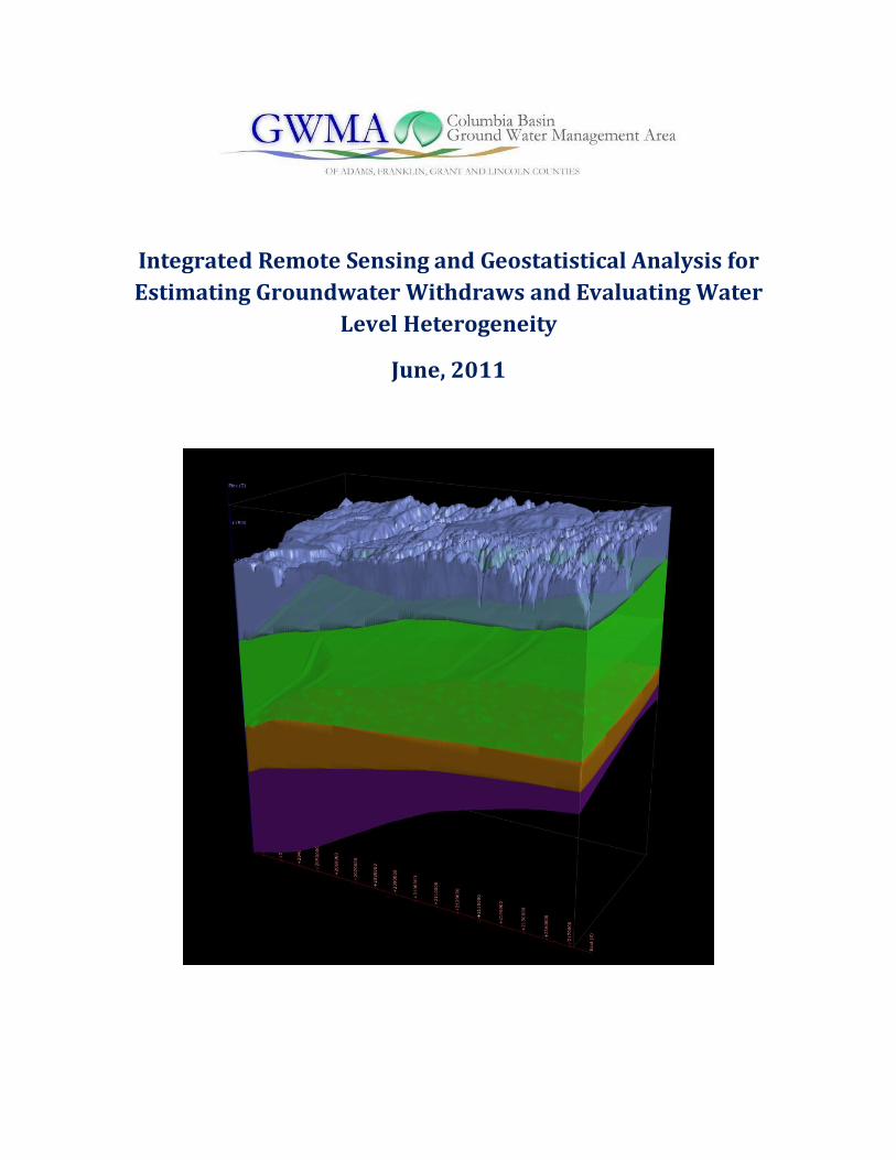
static groundwater level in a 21,500 km2 area underlain by the Columbia River Basalt Group aquifer

system using a geostatistical model. Groundwater pumping, and other significant covariates were

analyzed in their relationship to static groundwater levels using a geographically weighted regression

(GWR) model with variables derived from a spatial data base that included static groundwater level data

from 780 groundwater wells, well construction characteristics, stratigraphy, and topography. This study

estimated groundwater pumping by reconstructing cropping patterns with a 6-band multispectral

signature derived from Landsat 7 Enhanced Thematic Mapper (EMT +). Derived cropping patterns and

estimated groundwater pumping - which accounted for variation and topographic drift in climate drivers

- compared favorably with field data, historical records and interview data. Expected and residual values

from GWR model were interpolated and mapped, highlighting distinct patterns of heterogeneity which

correlated with geologic features that are thought to influence the regional groundwater system.

Geographic Information Systems is a powerful tool for integrating hydrogeologic data sets and

visualizing trends, which would otherwise be extremely difficult to detect at similar spatial extent with a

systematic ground-based approach alone. The results of this work contribute to the GWMA's

understanding of hydrogeologic complexity and compartmentalized nature of confined aquifers in this

region.


1.0 Introduction

Arid and semiarid climes account for more than 45 percent of the terrestrial biosphere world-

wide, and rely on groundwater, often as the primary source, for domestic, municipal, and agricultural

uses. In many of these regions withdraws can easily surpass net recharge. The importance of

sufficiently characterizing geology and groundwater withdraws to understand the occurrence,

movement, and variability of groundwater is a core principle of hydrogeology, and crucial for developing

and managing water resources. As geographic scale increases, assessing groundwater conditions

invariably becomes more complex. Hydrogeologic features may contribute to compartmentalization of

aquifers resulting in sub basins with substantial variation in underlying physical aquifer configuration,

and key hydraulic drivers. As examined in this report, this is thought to be the case in the confined

basalt aquifer system underlying an area > 21,000 km 2 in central-eastern Washington, USA. In situ field

tests provide the most in depth and defensible framework for aquifer assessment and evaluating the

influence of physical features and processes on groundwater movement; however, creating such a

framework to implement field-based tools at a regional scale is cost and time prohibitive.

Integrated remote sensing and Geographic Information Systems (GIS) complex is a powerful

approach for handling complex arrays of hydrogeologic data, and can use thematic layers to create

geostatistical models. Origins of the most commonly used statistic to interpolate and estimate variation

of the value of random field in space can be traced back to subsurface exploration. Multivariate

approaches have been used in concert with GIS to assess the effect of a broad range of explanatory

variables on spatial-temporal variations in ground water (Moukana and Koike, 2008; Oh et al., 2011).

Hydrogeologic studies have applied probabilistic and multi-criteria decision analysis (Chenini et al. 2010;

Corsini et al., 2009), and sophisticated decision tree and analytic hierarchy process analysis (Chowdry et


al., 2009; Srivastra and Bhattacharya, 2006). Notably, a geospatial approach is often necessary to

highlight synoptic-broad scale changes in groundwater availability in arid and semi-arid regions (Rodell

et al., 2009; Moukana and Koike 2008).

In this study the GWMA used a 2 step approach to examine regional variation in water level

variation. First, we use remote sensing imagery to calculate groundwater withdraws from high-capacity

agricultural wells. And second, we used results from ground water withdraws in step one, as one of

several explanatory variables to create a geostatistical model that examines region-wide variation in

water level in relation to key drivers. We interpolated residual values from the model and highlight

local scale variation in static ground water level within a 21,500 km 2 region of the Columbia River Basalt

Group (CRBG) regional aquifer system in south-central Washington, USA. While previous studies have

modeled hydraulic head across the CRBG region as a whole, they have been developed at much coarser

scale than the approach we describe for this study (Snyder and Haynes, 2010; Davis, 2002; Bossong,

1999). Additionally, to our knowledge this is the first study that estimates pumping at the regional scale,

and uses this information to determine the sensitivity of variation in hydraulic head to the physical

configuration of aquifers and geologic barriers, while accounting for groundwater withdraws.

The CRBG regional aquifer system is the primary, and in many cases, the only source of water for

south-central Washington, and significant declines in groundwater over the past several decades is of

concern to water resource managers. Hydraulic properties of CRBG aquifers are laterally and vertically

complex (Drost and Whiteman, 1986; USDOE, 1988; Whiteman et al., 1994; Hansen et al., 1994; Tolan et

al., 2009). A number of independent local-scale groundwater investigations in the CRBG region have

noted that folds and faults affect the occurrence, and in some cases block or restrict lateral movement

of groundwater (Newcomb, 1961; 1969, Gephart et al., 1979; Oberlander and Miller, 1981; Lite and

Grodin, 1988; USDOE, 1988; Packgard et al., 1996; Tolan et al., 2009). Using an integrated geospatial


modeling approach, we endeavor to do a more comprehensive evaluation of these features on

groundwater movement than previously available. The subdivision of the watershed into nested sub

basins would have vast implications for water resource management in this area.

2. Overview of Study Area and Characterization of Prominent Geologic Features

The Columbia Basin Ground Water Management Area (GWMA) of Adams, Franklin, Grant, and

Lincoln Counties encompasses approximately 21,500 km2 in south-central Washington. (Figure 1). The

GWMA is nested in the northern portion of the CRBG, which covers a large part of Oregon, Idaho, and

Washington. The CRBG consists of a thick sequence of more than 300 continental tholeiitic flood basalt

flows that cover an area of more than 152, 800 km2 (Tolan et al., 1989), and has been divided into a host

of regionally mappable units. CRBG basalt flows erupted during a period from about 17 to 6 million

years ago from long (6 to 30 mile) north-northwest-trending linear fissure systems located in eastern

Washington, northeastern Oregon, and Western Idaho. The surficial and subsurface manifestation of

these linear vents system are feeder dikes, which results when lava solidifies in the vent following flow

unit emplacement.

This region has been under a general north-south compression/east-west extension stress

regime from at least the beginning of CRBG time (Davis, 1981; Meyers and Price, 1979; Reidel et al.,

1982, 1989; Watters, 1989) to present-day (USDOE, 1988; Geomatrix, 1988; 1990), leading to a series of

folds and faults. Within this deformation regime The GWMA is divided into 2 general sub-provinces

which are important in characterizing fold, fault, and dike controls of ground water occurrence and

movement. The Yakima Fold Belt comprises the western one-quarter of the CBGWMA, and is

characterized by a series of northeast-trending faults, accompanied by abrupt changes in fold geometry

along the length of the folds (Swanson et al., 1979; Bentley et al. 1980, Reidel 1984; Figure 2). The


Palouse Slope is a structural province that comprises much of the eastern 3/4 of the CBGWMA. The

Palouse Slope is a regional dip slope (<1 to 2 degrees). Across this structural province stratigraphic dip

slightly exceeds the topographic slope. Deformation on the Palouse Slope is primarily characterized by

north to northwest trending and several east-west trending folds with little topographic expression

(Swanson et al., 1980; Tolan and Reidel, 1989).

The locations and extent of many of the folds, faults, and feeder dikes that cross-cut the GWMA

are fairly well know. Several decades of geologic mapping provide baseline maps for these geologic

features throughout the region (Gulick and Compiler, 1990; Gulick and Compiler, 1994; Gulick and

Korosec, 1990; Reidel, 1998; Rediel and Fecht, 1994; Figure 2). Composite maps are also available

through Washington Department of Natural Resources, Division of Geology and Earth Sciences

(http://www.dnr.wa.gov/ResearchScience/GeologyEarthSciences/Pages/Home.aspx). For this study,

generalized maps depict the general extent of features (folds, faults and dikes) that are currently though

to have the most influence on lateral hydraulic continuity within the CRBG aquifer system in the project

area (Lindsey et al., In Review; Figure 1). Spatially-extensive folds and faults, and we also believe dike

systems, play a significant role in forming a laterally compartmentalized aquifer system (Figure 2).

3. Methods

3.1 Estimating groundwater pumping

Groundwater pumping for all high-capacity (> 9 inches in well diameter) agricultural wells was

estimated by analyzing Landsat 7 satellite spectral bands to determine cropping patterns in concert with

Washington Irrigation Guide (WAIG) estimates for crop irrigation and consumptive water use per season

(http://www.wa.nrcs.usda.gov/technical/ENG/irrigation_guide). Once we established crop type and

irrigation requirement, groundwater pumping values were distributed to co-located agricultural wells.

Discharge per well was calculated using an empirical relationship total volume of pumping and well

http://www.dnr.wa.gov/ResearchScience/GeologyEarthSciences/Pages/Home.aspx


diameters (Fetter, 2001), such that groundwater pumping was apportioned by well diameter across the

spatial magnitude of each microclimate. Landsat data was classified by crop type for the summers crops

of 2000, 2001, 2002, and 2003. All thought we did not analyze data for each year independently for

separate set of analyses, several years were used in order to determine the dominant crop type for each

field. The major process steps were: 1) identification of a sample of crops growing at the time a satellite

image is being acquired; 1) acquiring and preparing the images, including determination of the best time

period during the growing season and number of images to use per classification; 2) identification of

crops growing at the same time the satellite image was acquired - verified by field based assessment 3)

developing distinctive signatures of the sampled crops based on spectral histograms and plots; and 4)

processing the classification, determining specific field classifications and creating a test matrix to

quantify results. An initial step to determine which crops could be distinguished using satellite images

was made using a Crop Curve, comparing the crop water use coefficient to seasonal dates. The Crop

Curve was used to determine those time periods when there were major differences in vegetation

growth between crops, thus increasing the software͛s ability to distinguish between crops. For example,

the Crop Curve showed the likely periods when alfalfa would be cut, when wheat would be harvested,

when potatoes would have full vegetation, and more importantly, when these periods occurred relative

to each other.

A subset of the crop fields were selected for ground reference (as noted in step 1). Fields to be

used as ground reference were selected based on size, location to a main road, and crop. A driving

route along secondary paved roads was identified, and an initial drive in early May identified fields along

the route that were greater than 40 acres, easily viewed from the road and contained (or were to

contain) crops to be classified. Crops were identified in the same fields along this route for each time

period of a selected satellite image. The number of fields required as ground reference for satellite


classification varies somewhat by crop, but refinement of the field sampling methods over the life of the

project, indicates approximately 8-10% of the expected crop acres should be visually identified for use in

image processing. This is necessary to account for the reflectance differences caused by crop species

variability, differences in crop growth stages (caused by location and management decisions), and

changes in crops through the season (double-cropping).

Landsat-ETM+, 30-meter resolution images were acquired for dates ranging between February

16, 2000 and July 10, 2003. For each crop season a minimum of 2 images (and up to 5 images in a single

season) were selected. The time step between images was consistent with the Crop Curve, and selected

when phenological characteristics of crop type, and remote sensing spectral counterpart, was most

discernable. Several combinations of images from different time periods were tested to determine an

optimum number and time period combination to produce the best classification. Supervised

classification techniques using areas of interest (AOI) were developed using ERDAS (ERDAS Inc., Atlanta,

GA, USA.) with spectral bands 1-5, and 7 (blue: 450-520 nm, green: 520-600 nm, red: 630-690 nm, Near

Infrared: 770-900 nm, Short-wave Red: 1,500-1750 nm, and shortwave Infrared 2,090-2350 nm).

Classes generated from AOIs were evaluated using plots of the mean pixel values per spectral band, and

histograms of band data values. Classification was done for each region of the image using the signature

file created for that region using a Maximum Likelihood decision rule.

Calculations for crop irrigation and consumptive water use were made per season per crop. As

our study area encompasses an elevational and climatic gradient where changes in atmospheric forcing

fluctuate over short distances (i.e. evapotranspiration, windspeed, water vapor deficit) accuracy of

water use parameters was increased throughout the study area by sub-dividing it into distinct separate

microclimate zones. Water use (acre feet year-1) was distributed per well in each micro-climate based.


Water use per well varied based on an empirical relationship between the well diameter and total

number of wells per each microclimate.

3.2 Spatial modeling of static water level

We used static water level data taken subsequent to 2003 from 338 Eastern Regional Office

(ERO) wells and 405 wells from the Department of Ecology (DOE) well data base to highlight local-scale

(<= 10 mile) variability, and evaluate sub-regional water level trends and discontinuities in relationship

to major geologic structures (Figure 1). The first stage of the process involved developing a predictive

regression model in regional ground water elevation trends using GWR analysis, where the dependent

variable; static ground water level elevation, was predicted using groundwater pumping and other

significant covariates. The second stage consisted of residual-krigging, where we krigged baseline static

water level values and added GWR residuals (the difference between observed and predicted static

water level) for a composite static water level map across the region. The third stage involved

transformation of interpolated residuals values alone in to continuous trend of 100 ft2 resolution as

values deviated from mean residuals. The resulting residual values map, scaled by standard deviation

from mean residual, were masked to the extent of the study area, and examined in relationship with

observed prominent geographic features. For this study we considered information on the folds, faults

and dikes (Figure 1) that are mapped in region, and created generalized structural bounding features,

which we used as a hypothesized baseline sub-basin boundaries.

Eastern Regional Office wells in the CBGWMA were selected from a broader sample of

monitoring wells Department of Ecology (DOE); for details see

http://www.ecy.wa.gov/programs/eap/groundwater/programdescription.html). From the total 816

wells monitored within Washington State 338 of these wells were located within the GWMA study area


and could be reliably reconciled with well construction details from DOE well log database. Selected

wells from ERO database alone (n=338) provided adequate sample size to draw inferences to the

population of water wells within the study area (based on statistical sampling theory; Yaneme et al.,

1967) However, wells from this data set alone exhibited significant clustering and were not evenly

distributed to the extent of the study area. This was particularly important for this study in areas that

were co-located with prominent geological features. Preliminary evaluation of interpolation using

"leave one out cross validation" method suggested predictive modeled ground water data was not

statistically reliable, and increasing level of error was observed beyond the central region of the study

area where wells were heavily concentrated. For the aforementioned reasons, we included additional

static water level data taken as recorded from driller͛s logs (n=405; Figure 1). Static water level

elevations from driller͛s logs were filtered for similar months (non-pumping season; November-March),

consistent with the timing of ERO static water level measurements. The inclusion of static water level

data from drillers log vastly improved our ability to interpolate to the extent of the GWMA, as well as

improving data spatial clustering and predictive capabilities of raw static water level data.

An explanatory model developed instead of examining static water level data directly in order to

evaluate differences in static water level elevation leveraged by ground water pumping, as well as other

potentially important covariates; elevation of land surface, elevation of basalt layer, well depth, depth of

casing. Geographically weighted regression builds a local regression equation for each feature in the

dataset, and builds separate regression equations by incorporating the dependent and explanatory

variables of features falling within the bandwidth of each target feature, depending on user input

(bandwidth, kernel type, distance ect.; Fotheringham et al., 2002). Using a GWR model for explanatory

data analysis is robust to data that exhibits spatial-autocorrelation and non-stationarity, which is often

the case in spatially explicit data sets (Preston and Brakebill, 1999). GWR permits parameter estimates


to vary locally (Brudson et al., 2000; Fatheringham et al., 2000), whereas an ordinary regression model

assumes that model structure remains constant through the study area.

Initially ordinary least squares method was used to isolate the significant variables and develop

the most parsimonious model for explaining the variation in static water levels. In addition to

groundwater pumping, possible covariates included continuous variables (surface elevation, elevation at

top of basalt, elevation at the bottom of seal, groundwater pumping, well depth) and nominal variables

( major open interval - Grande Ronde Basalt, Wanapum Basalt, Saddle Mountains Basalt, and/or

Sediment, or multiple). The relationship between covariates and response variables was evaluated for

multicollinearity by examining matrix plots for all variables (Table 1). An adaptive kernel type was used

for the GWR model, which was the basis for the spatial context (the Guassian Kernel) is a function of a

specified number of neighbors. Akaike Information Criterion (AICc) was used to determine the extent of

the Kernel.

4. Results

4.1 Remote sensing and groundwater pumping estimates

Using 6 spectral bands from remote sensing data classifications were made for 10 crops, with

included dominant - high water use - crop types for the regions (Figure 3 and 4b). Total acres by crop

type (i.e. potato, irrigated wheat) across the entire CBGWMA were consistent with expectations and

records from the United States Department of Agriculture for a subset (~ 2,500 km2 in the southern

portion) of our total study area. The preliminary Crop Curve analysis indicated that the most efficient

temporal pairing of images for extracting definitive crop signatures was in early to mid-May and late

June. Although there was significant deviation in mean pixel value for most spectral bands by individual

crops in the early season (May), this deviation was muted considerably as crops matured (as illustrated


for corn; Figure 3a). in June. Additionally, histograms of individual sample values followed an

approximately normal distribution, and could be reliably reconciled to individual crop type (Figure 3b).

Crops that could not be differentiated by 6-band spectral signatures in May, such as alfalfa and grass,

were reconcilable in late season (Figure 3c).

An overlay of fields classified by field type spatially correlated with production wells indicated

that the spatial extent of wells and well density at smaller scales (<20 km2) was adequate for

extrapolating pumping volumes (Figure 4b). Examination of wells by pumping volume was in good

agreement with spatial heterogeneity of co-located fields, and generally, with well pumping per field

acres (Figure 4c). The study was limited however, by the number of wells that actually appear in the

DOE well database (i.e. not to include unregistered wells); hence, wells may exist in areas where wells

do not appear, resulting in smaller areas where wells may be underrepresented with wells per number

of irrigated acres.

At the scale of the entire study area, total ground water pumping ranged from approximately

18,000 acre feet to 242,000 acre feet, corresponding to 71 to 310 production wells (253 to 780 acre feet

per year/ per well) respectively, per each microclimate (Figure 5). Predicted pumping volume per

microclimate deviated, as expected, based on hydro-meteorological growing conditions along the

elevation gradient, total number of irrigated acres, and by predominant crop type per region. In the far

northern portion of the GWMA, where fewer acres are irrigated proportionally, annualized precipitation

is higher and water vapor deficit is lower, a much lower pumping volume per total land area was

observed (Figure 5). In the microclimate in the western portion of the GWMA ("Quincy" microclimate;

Figure 5a), the total number of wells and total groundwater pumping is high, but the average volume

pumped per well is low. This relationship was expected because of predominant water saturated

suprabasalt (sediment and clay layers) in this region, which resulted in a high density site for production


wells, but fewer irrigated acres per well, and lower mean pumping per well (Figure 5). And in the

Odessa microclimate in the central-northern region, maximum ground water pumping is observed,

consistent with regional-based knowledge and scientific evidence of number of wells, productivity, and

declining water levels (Porcello et al., 2009; Snyder and Haynes, 2009; Vlossopoulos et al., 2009).

4.2 Regional variation in static water level

Wells from multiple data sources were well distributed throughout the GMWA provided the

basis for adequate spatial extent for interpolation of static water level data at observed locations, and

interpretation of variation in water level relative to geologic features. Results from "leave one out cross-

validation" statistical test suggested that the inclusion of wells from the DOE database improved the

interpolation significantly. Mapped results from our model provided a geographically extensive

framework for isolating trends that corroborate field-based evidence and interview data Initial analysis

using OLS to determine useable variables for GWR explanatory model indicated, that after accounting

for groundwater pumping, significant covariates included; the major unit that wells are sealed to, well

depth, elevation of land surface, and elevation of basalt surface (table 1). Two covariates - land surface

elevation and basalt surface elevation - exhibited multicollinearity with respect to relationship to

expected groundwater level. For the most parsimonious model we used top of elevation of basalt

alone, as top of basalt (elevation at top of basalt) was also the most highly correlated explanatory

variable. Regional scale static water-level maps, which included composite values of initial interpolation

and krigged residuals, ranged from 311 feet (amsl) to 2427 feet (amsl), and exhibited general northeast

by southwest trend, with notable dipping in the central to northern-central area (Figures 6a)),

consistent with observed water level declines in this regions (Porcello et al., 2009; Snyder and Haynes,

2010).


Residual values - the difference between each observed water level elevation and the predicted

water level elevation based on the GWR model - were normalized by a standard deviation scale and

interpolated to the bounding extent of outer most locations (Figure 6b). Water level values predicted by

GWR that deviated <> 1 StDev from average residual values were portrayed in hues of blue and red.

Contrasting patterns generally characterized water level continuity, highlighting areas of sharply

contrasting values. Salient trends were not always uniform along inferred hydrologic boundary and

often muted at coarser spatial resolution, but were characteristically strong in areas where fold and

faults systems were profound (Figure 2 and 6b). Lateral discontinuities, suggested by variation in

thematic map (Figure 6b), was consistent with existing local hydrologic evidence in many areas (Porcello

et al., 2009; Snyder and Haynes, 2010) , and also consistent with ad-hoc information and interviews .

(Paul Stoker, Personal Communication) In some cases contrasting patterns in nearby, contiguous areas

resulted from individual or small groups ч 3 of wells, and hence, patterns were speculative based on

sample size in these areas. However, in other areas adjacent to geologic features there was a strong

signature coming from many co-located wells suggesting that the trend was not an artifact of a small

group of outliers, but a strong case for lateral discontinuity influenced by geologic configuration and

hydrogeologic barriers.

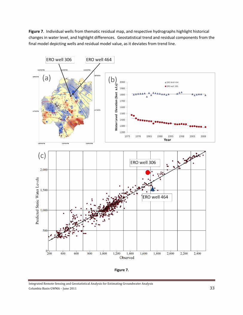
Although an exhaustive review of individual wells is beyond the scope of his study, a brief

supplemental analysis of a specific case-study corroborates the immediate interpretation of thematic

maps. The northwest by southeast tending dike systems in the northeastern portion of the study area

appears to influence adjacent water levels on either side of the dike. This is illustrated in mapped

results by the higher residual values northeast of the dikes system, and lower residual values to the

southwest of the dike system (Figure 7a). Moreover, this pattern does not stem from a single well, but

several wells in the vicinity, on either side of the dike system. Randomly selected wells on either side of


the within a relatively close proximity (< 7 miles) , exhibit distinct differences in terms of long-term static

water levels from 1973 to present (as noted by the comparison of 2 wells; ERO 306, and ERO well 464,

Figure 7b). Importantly, we have accounted for topographic differences in our model, thus variation in

water level cannot be attributed to differences in water level related to surface elevation alone. The

scatter plot depicting trend and residual components of our geostatistic model illustrates residual values

of each well, and their relative deviation from mean values (Figure 7c).

5.0 Discussion

Geographic Information Systems is a powerful tool for handling spatial data sets and can be

easily used to develop an integrated view of information from a broad range of geospatial repositories.

Results here draw from static ground water level and well construction data from over 700 groundwater

wells, while accounting for other significant covariates. Foremost, the integrated thematic model

results provide a framework for evaluating variation in static ground water level, and suggest that a

some of the lateral hydraulic continuity observed, may be related to prominent folds, faults and dike

systems. This information is of widespread interest to stakeholders and water resource managers, and

also of inherent interest to ground water modelers that must quantify and qualify boundary conditions

in order to delineate sub basins. Of socioeconomic and geopolitical interest, the primary agency

directing this study (GWMA) is locally based, and has participated in extensive public outreach and

public education seminars. Such opportunities for public interface have provided abundant

opportunities to assess and improve our analyses and build key networks of personal communication.

Similar GIS-based groundwater studies have found tremendous utility in using personal judgment and

local information to assign weight to geospatial data (Madrucci et al., 2008; Mondal et al., 2008;Yeh et

al., 2009).


The resolution our analysis, and the well-to-surface interpolation ratio developed in this study,

780 groundwater wells covering 26,000 km2 - approximately 1 well per 10 mi2, surpasses that of recent

studies in other the CRBG (Snyder and Haynes, 2010). Mapped results rendered from interpretation of

results provide a general template for isolating and examining wells and regions of interest for further,

more in depth analysis (Figure 6b). The inclusion of field-based data for mapping predominant fold,

fault and dike systems, is arguably better than similar GIS approaches where lineament maps have been

produced by interpreting satellite images with hillshade maps (Koike et al., 1998; Kumar et al., 2009;

Hyun-Joo et al., 2011). Hence the interpretation of variation in water level alone, after accounting for

groundwater withdraw and physical features, may be linked to the influence of those features on

ground water, if (and where) these features do influence the occurrence and movement of

groundwater. However, our evaluation here, although helpful in recognizing regional scale trends and

discontinuities, is only an initial step in that process. Ideally, variation in our modeled results would be

further corroborated with field-based well testing, including implementation of a long term observation

well program.

In addition to mapping static ground water level elevations and variation, our results provide the

most current and comprehensive estimation of groundwater withdraws in this region of the CRBG.

Groundwater pumping is a challenging component of the groundwater budget to estimate as it requires

either participation from well owners, or estimation of pumping using indirect parameters. Although,

remote sensing has been used to calculate water use requirements in experimental irrigated agriculture

plots with a single crop type (Thorp et al., 2010; Hunsaker et al., 2005), these results have not

necessarily been extended beyond the research scenario, to the regional scale, with comparable

precision. Noteworthy advancements have been made using remote sensing to establish baseline

estimates of water use at local, regional, and global scales (Thenkabail et al., 2008). While useful, many


cropland maps at coarser resolution are limited by absence of precise spatial location, absence of crop

types, and differentiating between irrigated crops and rain fed crops. We are fortunate, that in the

region of the CRBG we evaluate, that center-pivot irrigation evolved concurrently with ground water

pumping. Hence, plots irrigated from ground water are generally circular since the 1960's (Figure 4).

This facilitates classification of irrigated verses rain fed crop fields.

For direct pumping assessment, records may be acquired from municipalities and domestic well

users; however, these sources collectively account for only a small fraction (< 5%) of the water used by

major agricultural producers. Hence, ground water pumping estimates from these sources alone cannot

be inferred to the general population of wells, and reliable information from high-capacity wells is

necessarily collected independently of municipal and domestic wells. Studies drawing from a smaller

geographic area and sample size, have used both power coefficient term (PCC) and/or totalizing

flowmeter (TFM) to calculate groundwater pumping (Troutman et al., 2005; Dash et al., 1999; Hansen et

al., 1994; Cline and knadel, 1984). We obtained comparable results using a remote sensing crop - water

use approach, but as discussed here, neither the PCC or TFM techniques are appropriate in our study.

The PCC method relies on an algorithm developed using the interdependent relationship between

electrical consumption and groundwater withdraw. The totalizing TFM is a direct measurement of the

volume of water discharged, and is, ostensibly, the most accurate measurement. Although estimated

pumping rates compare favorably with instantaneous measurements from both methods (Dash et al.,

1999), Troutman and colleagues (2005) found that when using PCC method for an entire year, the

pumpage computed with the PCC approach tended to be less than pumpage using TFM, and

discrepancies increased with a forward-trending time lag. Supplemental analysis revealed significant

correlation with dynamic groundwater level and the linear relationship between the PCC approach and

TFM approach in time trend analysis (Troutman et al., 2005). The effect of groundwater level on the


PPC estimated values is expected to vary based on the relationship between aquifer configuration and

the amount of mechanical work required to pump water to the surface, and the depth of water from the

land surface. Although this source of error may be muted in unconfined aquifers and suprabasalts, it is

exacerbated in our area of study, where wells are often cased > 1000 feet down to confined basalt

layers, and dynamic water level is > 500 feet below ground surface. Indeed we found, based on the only

study known to us in the CRBG using PCC to calculate ground water withdraws, that the PCC method

estimated less pumpage per well than our crop based estimates; 236 acre feet per well on average in

nearby (Hansen et al., 1984), compared to 253 acre feet per well in areas of highest precipitation

regime locally, and to 780 acre feet per year in areas of lowest precipitation regime locally in our study.

An additional discrepancy to consider with aforementioned techniques used to estimate ground

water withdraw, is that total pumping is generally divided among the total or aggregate network of wells

for which the measurement is taken irrespective of well construction. For example if 10 wells draw

electrical power from a single source, each well is assumed to pump equal amounts, even if one is a

shallow domestic well, and one is a deep irrigation well. This may have undesirable consequences for

both the variance in estimation of water pumped per well, and the amount of water applied at specific

fields. By developing and accessing a geospatial well database, we account for well construction, and

differences in the magnitude of ground water pumping on a well-by-well basis. Using a crop-based

approach we gain the additional insight with respect to water applied per field, which has a suite of

advantages if one is to use information for developing conceptual and/or numerical groundwater

models.


6.0 Conclusion

Water resource management and regulation is becoming increasingly complex in arid and semi-

arid climes that rely on groundwater, which is often unsustainable and often being used at a rate that

exceeds recharge. Understanding variation in groundwater elevation across landscapes has emerged as

a research priority, and is germane to future management of water resources at regional scales.

In this study we employed an integrated view using GIS, developed in combination with

geographical, geological and hydrogeological factors, in order to assess region wide groundwater

resources. Conventional hydraulic head maps, derived at coarse watershed scales, do not necessarily

account for variation that is critical in evaluating water budgets, hydrogeologic processes, and water

rights. Our study is the first in this region to i) estimate groundwater pumping by cropping patterns at

this scale, and ii) evaluate regional scale heterogeneity in groundwater elevations with the inclusion of

key covariates that play a role in driving variation. Our results compare favorably with field-based

observations and interview data; however, our work also warrants future corroboration with

geographically extensive field surveys.


ACKNOWLEDGEMENTS

This research has been supported through a Washington State Legislative Proviso in the 2009-

2011 Capital Budget Appropriations, via Washington State Department of Ecology. We extend our

gratitude to the Boards of County Commissioners of Adams, Franklin, Grant and Lincoln Counties for

their continued oversight and support of the GWMA; to the members of the GWMA Administrative

Board for their guidance; and to the local citizens and stakeholders of the four-county area who have

participated and provided invaluable information and feedback for the GWMA.

LITERATURE CITED

Bentley, R. D., 1977. Stratigraphy of the Yakima basalts and structural evolution of Yakima ridges in the western Columbia Plateau.; Geologic Excursion in the Pacific Northwest, Western Washington University

Brunsdon, C., Aitkin, M., Fotheringham, A.S., and Charlton, M.E., 2000. A comparison of random coefficient modelling and geographically weighted regression for spatially non-stationary regression problems. Geographical and Environmental Modelling 3(1), 47-62

Cline, D. R. and Knadle M. E., 1984. Ground-water pumpage from the Columbia Plateau Regional Aquifer System. U. S. Geological Survey. Water Resources Investigation Report 87-4135.

Davis, G. A., 1981. Late Cenozoic tectonics of the Pacific Northwest with special reference to the Columbia Plateau:Richland, Washington, Washington Public Power Supply System Final Safety Analysis Report for WPN-2, appendix 2.5N, 44p.

Drost, B. W., and Whiteman, K. J., 1986. Superficial geology, structure, and thickness of selected geohydrologic units in the Columbia Plateau Regional system. Washington: U.S. Geological Survey Water-Resources investigation Report 87-4238.

Fetter, C. W. 2001. Applied Hydrogeology (Fourth Edition). Prentice Hall, New Jersey.

Fotheringham, A.S., Brundson, C., and Charlton M., 2002. Geographically Weighted Regression: The Analysis of spatially varying relationships. Wiley and Sons, New York.

Gephart, R. E., Arnett, R. C. Baca, R. G., Leonhart, L. S., Spane, F. A., Jr., 1979. Hydrologic Studies withinthe Columbia Plateau , Washington- and integration of current knowledge: Richland,Washington, Rockwell Hanford Operations, RHO-BW1-ST-5.


Gulick. C. W., 1990a. Geologic map of the Moses Lake 1:100,000 quadrangle, Washington: Washington Division of Geology and Earth Resources Open File Report 90-1, 9 1 plate.

Gulick. C. W., 1994a. Geologic map of the Connell Area 1:100,000 quadrangle, Washington: Washington Division of Geology and Earth Resources Open File Report 90-14, 9 1 plate.

Gulick , C. W., 1990. Geologic map of the Banks Lake 1: 100,000 quadrangle, Washington: Washington Division of Geology and Earth Resources Open Source File 90-6, 20p., 1 plate

Hansen, A. J., Vaccaro, J. J. and Bauer, H. H., 1994. Ground-water flow simulations of the Columbia Plateau regional aquifer system, Washington, Oregon, and idaho: U.S. Geological Survey, Water Resources investigation Report 91-4187, 81. p

Hunsaker, D. J., Pinter P. J., Barnes E. M., and Kimball, B. A, 2003. Estimating cotton evpotranspiration crop coefficients with a multispectral vegetation index. Irrigation Science 22, 95-104

Isaaks, E. H., & Srivastava, R. M., 1989. Applied geostatistics. Oxford University Press Inc, New York.

Karl, J. W., 2010. Spatial Predictions of Rangeland Ecosystems Using Regression Kriging and Remote Sensing. Rangeland Management 63, 335-349

Koike, K., Nagano, S., Kawaba, K., 1998. Construction and Analysis of Interpreted fracture planes through combination of satellte-image dervied lineaments and digital elevation model. Computers and Geoscience 24, 573-583

Kumar, M. C., Bali, R. Agarwal, A. K., 2009. Integration of remote sensing and electircal sounding data for hydrogeologic exploration - A case study of Bakhar Watershed, India. Hydrogeological Sciences. 54, 949-960.

Kovitz, J. L., & Christakos, G., 2004. Spatial Statistics of clustered data. Stochastic Environmental Research 18, 147-166.

Lite, K. E. and Grodin, G. H., 1988. Hydrogeology of the basalt aquifers near Moiser, Oregon - a ground water resources assessment: Oregon Department of Water Resources Ground Water Report, no. 33, 119 p.

Moukana, J. A., and Koike, K., 2008. Geostatistical model for correlating declining groundwater levels with changes in land cover detected from analyses of satellite images. Computers and Geoscience 34, 1527-1540.

Newcomb, R. C. (1961). Storage of ground water behind subsurface dams in the Columbia River basalt, Washington, Oregon, and Idaho: U.S. Geological Survey Professional Paper 238A, 15 p.


Oberlander, P. L. and Miller, D. W. (1981). Hydrologic studies in the Umatilla structural basin - an integration of current knowledge: Oregon Department of Water Resources, unpublished preliminary report, 41 p.

Oh, H., Kim Y. S., Choi J. K., Park E., and Lee S., 2010. GIS Mapping of Regional Probabilistic Groundwater Potential in the Area of Pohang City, Korea. Journal of hydrology 399, 158-172

Reidel, S. P., 1988. Geologic map of the Saddle Mountains, south-central Washington: Washington State Department of Natural Resources, Division of Geology and Earth Resouces GMS-38, 5 Plates.

Saraf, A. K., Choudhury, P. R., Roy. B., Sarma B., Vijay S., Choudhury, S., 2004. GIS based surface surface hydrological modeling in identification of groundwater recharge zone. International Journal of Remote Sensing 25, 5759-5770.

Snyder, T. S., and Haynes, J. V., 2010. Groundwater Conditions During 2009 and Changes in Groundwater Levels from 1984 to 2009, Columbia Plateau REgional Aquifer System, Washington, Oregon, and Idaho. Scientific Investigations Report 2010-5040. United States Geological Survey.

Thenkabail, P. S., Biradar, C. M. Noojipady, P., Dheeravath, V., Li, Y. J., Reddy, G. P. O., Cai, X. L., Gumma, M., Turral, H., Vithanage, J., Schull, M., and Dutta R. 2008. A Global irrigated area map (GIAM) using remote sensing at the end of the last Millennium: International Water Management Institute.

Thorp, K. R., Hunsaker, D. J., and French, A. N., 2010. Assimilating Leaf Area index Estimates From Remote Sensing into Simulations of A Cropping System Model. Transactions of the ASABE 53, 251-262.

Truman, B. M., Edlemann, P., Dash R. G., 2005. Variability of Differences between two approaches for determining ground-water discharge and pumpage, including effects of time trends, low Arkansas River Basin, southeastern Colorado, 1998-2002. United States Geologic Survey. Scientific Investigations Report 2005-5063.

Yaname, T. , 1967. Elementary sampling theory. Prentice-Hall, New Jersey.


TABLE


Table 1. Parameter from estimates from initial OLS output present day static water levels. Parameters were considered significant at an alpha level of 0.05. a,bParameters that exhibit multicollinearity in their collective relationship to static water level elevation ranked (from a-c) in order of Pearson's r coefficient.

Term Estimate Std Error t Ratio Prob > /t/

Intercept -399.26 174.02 -2.29 0.024 Primary unit sealed to [GRB] -644.89 284.17 -2.26 0.026 Primary unit sealed to [WB] -452.89 235.00 -2.50 0.08 Primary unit sealed to [GRB and WB] 339.687 149.67 2.26 0.026 Well Depth -0.289 0.0343 -8.44 2.02E-12 a Elevation at top of basalt 3.24 0.62 20.63 1.65E-07 b Elevation at land surface 2.24 0.50 4.44 3.03E-05

Table 1.


FIGURE LEGENDS


Figure 1. Study outline in central-eastern Washington, USA depicting topographic relief, wells used in this study from the 2 primary databases, and generalized hydrogeologic barriers. Data from wells include 338 Eastern Regional Office (ERO), Department of Ecology Subdivision, and 405 wells from Department of Ecology Well Database. ERO wells have an ongoing database of static water measurements taken annually since 1980. DOE well database gives a record static water level at the time of drilling. Generalized hydrogeologic barriers map for this study that depicts the general extent of features (folds, faults and dikes) that are currently though to have the most influence on lateral hydraulic continuity within the CRBG aquifer system in the project area (Lindsey et al. Unpublished). Many of the lineament features directly overlay folds and faults (See figure 2), and correspond with linear extending dike vents, and dike outcrops.

Figure 1.


Figure 2. (a) Depiction of folds and faults in the southwestern quarter of the GWMA study area. Lines shown here are the results of several decades of intensive geologic mapping which provide baseline maps for these geologic features throughout the region (Gulick and Compiler 1990, Gulick and Compiler 1994, Gulick and Korosec 1990, Reidel 1998, Rediel and Fecht 1994). (b) A fence diagram from the same area depicting multiple different interflow zones. Fence was taken from actual physical configuration of aquifers (Lindsey and Tolan 2009), which are also the underlying basis for interpolating static water levels in this study. The primary fold in the fence illustrates the discontinuous nature of the water bearing interflow zones moving from north to south along the north-south axis of the fence diagram. Evidence from borehole logs is used to indicate depth and configuration of basalt surfaces, and the discontinuous nature correlated with these features.

Figure 2.


Figure 3. Remotes sensing evaluation of crop type. Spectral means and StDev for 7 individual bands for corn from Landsat images acquired in May and June (a). Histogram for pixel values from Landsat spectral band 4 (770-900 nm; b). Mean values for spectral means from 7 bands for dominant crop types throughout the GWMA study area (c).

Figure 3.


Figure 4. Crop classification results and interpolation of groundwater pumping. A subsection of the study area illustrating the RBG image over lay, crop classification by field boundaries, production wells (all wells from DOE data base with well diameter > 10 inches), and groundwater pumping interpolation. Results for this spatial subset show wells pumping between approximately 90 to 1200 acre feet per year, with variation in well pumping reflecting the average variation throughout the GWMA.

Figure 4.


Figure 5. Groundwater pumping by microclimate. Illustration of the CBGWMA and microclimates with proportional groundwater pumping volumes. The total number of wells per each microclimate, the total pumping volume, and the average and StDev per well.

Figure 5.


Figure 6. Water table elevation from throughout the study area interpolated from all wells using a residual krigging technique (a). Shades of blue are contoured at approximately 300 to 400 feet. Generalized lineament map. Folds, faults and dikes from extensive geophysical surveys, and are generally correlated with top of basalt elevation at the same extent. Residuals values exceeding 1 StDev from mean residual illustrated in hues of blue (higher water elevation than expected) and red (lower water elevation than expected; b). Residuals shown here with major hydrogeologic features to illustrate possible spatial correlation.

Figure 6.


Figure 7. Individual wells from thematic residual map, and respective hydrographs highlight historical changes in water level, and highlight differences. Geostatistical trend and residual components from the final model depicting wells and residual model value, as it deviates from trend line.

Figure 7.

Documents

Integrated Remote Sensing and Geostatistical Analysis for ... · Integrated Remote Sensing and Geostatistical Analysis for Estimating Groundwater Withdraws and Evaluating Water Level