Embed Size (px)
Citation preview

Integer-Order Optimal Control Problems (IOOCP)A Tutorial and A Matlab Toolbox for Solving General IOOCP
(RIOTS 95)
YangQuan Chen, Senior Member, IEEE
MESA LAB (Mechatronics, Embedded Systems and Automation Lab)ME/EECS/SNRI/UCSolar, School of Engineering
5200 North Lake Road, University of California at Merced,Merced, CA95343, USA
ME280 Instructor: Dr. YangQuan ChenURL: http://mechatronics.ucmerced.edu
Email: [email protected] or [email protected]
9:00-10:15AM, Thursday, November 14, 2013. @ KL 217
Slide 1 of 69

What will we study?
• Part-1: (Integer-Order) Optimal Control Theory:
– The (Integer-Order) calculus of variations (a little bit)
– Solution of general (Integer-Order) optimization problems
– Optimal closed-loop control (LQR problem)
– Pontryagin’s minimum principle
Slide 2 of 69

What will we study? (cont.)
• Part-2: RIOTS 95 - General IOOCP Solver in the form of Matlab toolbox.
– Introduction to (Integer-Order) numerical optimal control
– Introduction to RIOTS 95
∗ Background∗ Usage and demo
Slide 3 of 69

1. Part-1: Basic Optimal Control TheoryWarming-up: A Static Optimization Problem
min : L(x, u), x ∈ Rn, u ∈ Rm
subject to: f (x, u) = 0, f ∈ Rn
Define Hamiltonian function
H(x, u, λ) = L(x, u) + λTf (x, u), λ ∈ Rn
Necessary conditions:∂H
∂λ= f = 0
∂H
∂x= Lx + fTx λ = 0
∂H
∂u= Lu + fTu λ = 0
Slide 4 of 69

What is an (Integer-Order) optimal control problem (dynamic optimization)?System model:
x(t) = f (x, u, t), x(t) ∈ Rn, u(t) ∈ Rm
Performance index (cost function):
J(u, T ) = φ(x(T ), T ) +
∫ T
t0
L(x(t), u(t), t)dt
Final-state constraint:ψ(x(T ), T ) = 0, ψ ∈ Rp
Slide 5 of 69

Some cost function examples
• Minimum-fuel problem
J =
∫ T
t0
u2(t)dt
• Minimum-time problem
J =
∫ T
t0
1dt
• Minimum-energy problem
J = xT (T )Rx(T ) +
∫ T
t0
{xT (t)Qx(t) + uT (t)Ru(t)
}dt
Slide 6 of 69
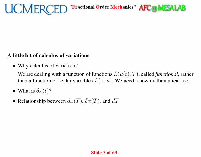
A little bit of calculus of variations
• Why calculus of variation?
We are dealing with a function of functionsL(u(t), T ), called functional, ratherthan a function of scalar variables L(x, u). We need a new mathematical tool.
• What is δx(t)?
• Relationship between dx(T ), δx(T ), and dT
Slide 7 of 69

Relationship between dx(T ), δx(T ), and dT :
dx(T ) = δx(T ) + x(T )dT
Slide 8 of 69

Leibniz’s rule:
J(x(t)) =
∫ T
x0
h(x(t), t)dt
dJ = h(x(T ), T )dT +
∫ T
t0
[hTx (x(t), t)δx]dt
where hx , ∂h∂x
.
Slide 9 of 69

Solution of the general optimization problem:
J(u, T ) = φ(x(T ), T ) +
∫ T
t0
L(x(t), u(t), t)dt (1)
x(t) = f (x, u, t), x(t) ∈ Rn, u(t) ∈ Rm (2)
ψ(x(T ), T ) = 0 (3)
Using Lagrange multipliers λ(t) and ν to join the constraints (2) and (3) to theperformance index (1):
J ′ = φ(x(T ), T ) + νTψ(x(T ), T ) +
∫ T
t0
[L(x, u, t) + λT (t)(f (x, u, t)− x)]dt
Note:ν: constant, λ(t): function
Slide 10 of 69

Define the Hamiltonian function:
H(x, u, t) = L(x, u, t) + λTf (x, u, t),
then
J ′ = φ(x(T ), T ) + νTψ(x(T ), T ) +
∫ T
t0
[H(x, u, t)− λT x]dt.
Using Leibniz’s rule, the increment in J ′ as a function of increments in x,λ, ν, u,and t is
dJ ′ = (φx + ψTx ν)Tdx|T + (φt + ψTt ν)dt|T + ψT |Tdν
+(H − λT x)dt|T+∫ Tt0[HT
x δx +HTu δu− λTδx + (Hλ − x)Tδλ]dt
(4)
To eliminate the variation in x, integrate by parts:
−∫ T
t0
λTδxdt = −λTδx|T +∫ T
t0
λTδxdt
Slide 11 of 69

Rememberdx(T ) = δx(T ) + x(T )dT,
so
dJ ′ = (φx + ψTx ν − λ)Tdx|T + (φt + ψTt ν +H)dt|T + ψT |Tdν
+
∫ T
t0
[(Hx + λ)Tδx +HTu δu + (Hλ − x)Tδλ]dt.
According to the Lagrange theory, the constrained minimum of J is attained at theunconstrained minimum of J ′. This is achieved when dJ ′ = 0 for all independentincrements in its arguments. Setting to zero the coefficients of the independent in-crements dν, δx, δu, and δλ yields following necessary conditions for a minimum.
Slide 12 of 69

System model:x = f (x, u, t), t ≥ t0, t0 fixed
Cost function:
J(u, T ) = φ(x(T ), T ) +
∫ T
t0
L(x, u, t)dt
Final-state constraint:ψ(x(T ), T ) = 0
State equation:
x =∂H
∂λ= f
Costate (adjoint) equation:
−λ =∂H
∂x=∂fT
∂xλ +
∂L
∂x
Slide 13 of 69

Stationarity condition:
0 =∂H
∂u=∂L
∂u+∂fT
∂uλ
Boundary (transversality) condition:
(φx + ψTx ν − λ)T |Tdx(T ) + (φt + ψTt ν +H)|TdT = 0
Note that in the boundary condition, since dx(T ) and dT are not independent, wecannot simply set the coefficients of dx(T ) and dT equal to zero. If dx(T ) = 0(fixed final state) or dT = 0 (fixed final time), the boundary condition is simplified.What if neither is equal to zero?
Slide 14 of 69

An optimal control problem example: temperature control in a roomIt is desired to heat a room using the least possible energy. If θ(t) is the temperaturein the room, θa the ambient air temperature outside (a constant), and u(t) the rate ofheat supply to the room, then the dynamics are
θ = −a(θ − θa) + bu
for some constants a and b, which depend on the room insulation and so on. Bydefining the state as
x(t) , θ(t)− θa,we can write the state equation
x = −ax + bu.
Slide 15 of 69

In order to control the temperature on the fixed time interval [0, T ] with the leastsupplied energy, define the cost function as
J(u) =1
2s(x(T )) +
1
2
∫ T
0
u2(t)dt,
for some weighting s.The Hamiltonian is
H =u2
2+ λ(−ax + bu)
The optimal control u(t) is determined by solving:
x = Hλ = −ax + bu, (5)
λ = −Hx = aλ, (6)
0 = Hu = u + bλ (7)
Slide 16 of 69

From the stationarity condition (7), the optimal control is given by
u(t) = −bλ(t), (8)
so to determine u∗(t) we need to only find the optimal costate λ∗(t).Substitute (8) into (5) yields the state-costate equations
x = −ax− b2λ (9)λ = aλ (10)
Sounds trivial? Think about the boundary condition!
Slide 17 of 69

From the boundary condition:
(φx + ψTx ν − λ)T |Tdx(T ) + (φt + ψTt ν +H)|TdT = 0,
dT is zero, dx(T ) is free, and there is no final-state constraint. So
λ(T ) =∂φ
∂x|T = s(x(T )− 10).
So the boundary condition of x and λ are specified at t0 and T , respectively. This iscalled two-point boundary-value (TPBV) problem.Let’s assume λ(T ) is known. From (10), we have
λ(t) = e−a(T−t)λ(T ).
Slide 18 of 69

Sox = −ax− b2λ(T )e−a(T−t).
Solving the above ODE, we have
x(t) = x(0)e−at − b2
aλ(T )e−aTsinh(at).
Now we have the second equation about x(T ) and λ(T )
x(T ) = x(0)e−aT − b2
2aλ(T )(1− e−2aT )
Assuming x(0) = 0◦, λ(T ) can now be solved:
λ(T ) =−20as
2a + b2s(1− e−2aT )
Slide 19 of 69

Now the costate equation becomes
λ∗(t) =−10aseat
aeaT + sb2sinh(aT )
Finally we obtain the optimal control
u∗(t) =10abseat
aeaT + sb2sinh(aT )
Conclusion:TPBV makes it hard to solve even for simple OCP problems. In most cases, we haveto rely on numerical methods and dedicated OCP software package, such as RIOTS.
Slide 20 of 69

Closed-loop optimal control: LQR problemProblems with the optimal controller obtained so far:
• solutions are hard to compute.
• open-loop
For Linear Quadratic Regulation (LQR) problems, a closed-loop controller exists.
Slide 21 of 69

System model:x = A(t)x +B(t)u
Objective function:
J(u) =1
2xT (T )S(T )x(T ) +
1
2
∫ T
t0
(xTQ(t)x + uTR(t)u)dt
where S(T ) and Q(t) are symmetric and positive semidefinite weighting matrices,R(t) is symmetric and positive definite, for all t ∈ [t0, T ]. We are assuming T isfixed and the final state x(T ) is free.State and costate equations:
x = Ax−BR−1BTλ,
−λ = Qx + ATλ
Slide 22 of 69

Control input:u(t) = −R−1BTλ
Terminal condition:λ(T ) = S(T )x(T )
Considering the terminal condition, let’s assume that x(t) and λ(t) satisfy a linearrelation for all t ∈ [t0, T ] for some unknown matrix S(t):
λ(t) = S(t)x(t)
To find S(t), differentiate the costate to get
λ = Sx + Sx = Sx + S(Ax−BR−1BTSx).
Slide 23 of 69

Taking into account the costate equation, we have
−Sx = (ATS + SA− SBR−1BTS +Q)x.
Since the above equation holds for all x(t), we have the Riccati equation:
−S = ATS + SA− SBR−1BTS +Q, t ≤ T.
Now the optimal controller is given by
u(t) = −R−1BTS(t)x(t),
and K(t) = R−1BTS(t)x(t) is called Kalman gain.Note that solution of S(t) does not require x(t), so K(t) can be computed off-lineand stored.
Slide 24 of 69

Pontryagin’s Minimum Principle: a bang-bang control case studySo far, the solution to an optimal control problem depends on the stationarity condi-tion ∂H
∂u= 0. What if the control u(t) is constrained to lie in an admissible region,
which is usually defined by a requirement that its magnitude be less than a givenvalue?Pontryagin’s Minimum Principle: the Hamiltonian must be minimized over alladmissible u for optimal values of the state and costate
H(x∗, u∗, λ∗, t) ≤ H(x∗, u, λ∗, t), for all admissible u
Slide 25 of 69

Example: bang-bang control of systems obeying Newton’s laws:System model:
x1 = x2,
x2 = u,
Objective function (time-optimal:
J(u) = T =
∫ T
0
1dt
Input constraints:|u(t)| ≤ 1
Slide 26 of 69

End-point constraint:
ψ(x(T ), T ) =
(x1(T )x2(T )
)= 0.
The Hamiltonian is:H = 1 + λ1x2 + λ2u,
where λ = [λ1, λ2]T is the costate.
Costate equation:
λ1 = 0 ⇒ λ1 = constantλ2 = −λ1 ⇒ λ2(t) is a linear function of t (remember it!)
Boundary condition:λ2(T )u(T ) = −1
Slide 27 of 69

Pontryagin’s minimum principle requires that
λ∗2(t)u∗(t) ≤ λ∗2(t)u(t)
How to make sure λ∗2(t)u∗(t) is less or equal than λ∗2(t)u(t) for any admissible u(t)?
Answer:
u∗(t) = −sgn(λ∗2(t)) ={
1, λ∗2(t) < 0−1, λ∗2(t) > 0
What if λ∗2(t) = 0? Then u∗ is undetermined.Since λ∗2(t) is linear, it changes sign at most once. So does u∗(t)!
Slide 28 of 69

Since rigorous derivation of u∗(t) is still a little bit complicated, an intuitive methodusing phase plane will be shown below.Going backward (x1 = 0 and x2 = 0) in time from T , with u(t) = +1 or u(t) =−1, we obtain a trajectories, or switching curve, because switching of control (ifany) must occur on this curve. Why?
Slide 29 of 69

−50 −40 −30 −20 −10 0 10 20 30 40 50−10
−8
−6
−4
−2
0
2
4
6
8
10
x1
x2
Switching Curve
u=+1
u=−1
Slide 30 of 69

References:F. L. Lewis and V. L. Syrmos, Optimal Control, John Wiley & Sons, Inc, 1997A. E. Bryson and Y. C. Ho, Applied Optimal Control, New York: Hemisphere, 1975J. T. Betts, Practical Methods for Optimal Control Using Nonlinear Programming,SIAM, 2001I. M. Gelfand and S. V. Fomin, Calculus of Variations, New York: Dover Publica-tions, 1991
Slide 31 of 69

2. Part-2: RIOTS 95 - General OCP Solver in theform of Matlab toolbox
Numerical Methods for Optimization Problems
• Static optimization
– Status: well-developed
– Available software package: Matlab optimization toolbox, Tomlab, NEOSserver, . . .
• Dynamic optimization
– Status: not as “matured” as static optimization
– Available software package: SOCS, RIOTS, MISER, DIRCOL, . . .
Slide 32 of 69

Why Optimal Control Software?
1. Analytical solution can be hard.
2. If the controls and states are discretized, then an optimal control problem isconverted to a nonlinear programming problem. However . . .
• Discretization and conversion is professional.
• Selection and use of nonlinear programming package is an art.
• For large scale problems, direct discretization may not be feasible.
Slide 33 of 69

Classification of methods for solving optimal control problemsA technique is often classified as either a direct method or an indirect method.
• An indirect method attempts to solve the optimal control necessary condition-s. Thus,for an indirect method, it is necessary to explicitly derive the costateequations, the control equations, and all of the transversality conditions.
• A direct method treats an OCP as an mathematical programming problem afterdiscretization. Direct method does not require explicit derivation and construc-tion of the necessary conditions.
Slide 34 of 69

What is RIOTS?RIOTS is a group of programs and utilities, written mostly in C, Fortran, and M-filescripts and designed as a toolbox for Matlab, that provides an interactive environ-ment for solving a very broad class of optimal control problems.
Slide 35 of 69

Main contributions and features of RIOTS:
• The first implementation of consistent approximation using discretization meth-ods based on Runge-Kutta integration
• Solves a very large class of finite-time optimal control problems
– trajectory and endpoint constraints
– control bounds
– variable initial conditions and free final time problems
– problems with integral and/or endpoint cost functions
Slide 36 of 69

Main contributions and features of RIOTS: (cont.)
• System functions can supplied by the user as either C-files or M-files
• System dynamics can be integrated with fixed step-size Runge-Kutta integra-tion, a discrete-time solver or a variable step-size method.
• The controls are represented as splines, allowing for a high degree of functionapproximation accuracy without requiring a large number of control parameters.
Slide 37 of 69

Main contributions and features of RIOTS: (cont.)
• The optimization routines use a coordinate transformation, resulting in a signif-icant reduction in the number of iterations required to solve a problem and anincrease in the solution accuracy.
• There are three main optimization routines suited fro different levels of gener-ality of the optimal control problem.
• There are programs that provides estimates of the integration error.
Slide 38 of 69

Main contributions and features of RIOTS: (cont.)
• The main optimization routine includes a special feature for dealing with sin-gular optimal control problems.
• The algorithms are all founded on rigorous convergence theory.
Slide 39 of 69

History of RIOTS:1. RIOTS for Sun (Adam L. Schwartz)
• Compiler: Sun C compiler
• Matlab Version: Matlab 4
• MEX version: v4
Slide 40 of 69

History of RIOTS: (cont.)2. RIOTS for DOS and Windows (YangQuan Chen)
• Compiler: Watcom C
• Matlab Version: Matlab 4, 5
• MEX version: v4
Slide 41 of 69
History of RIOTS:(cont.)3. RIOTS for Windows (rebuild) and Linux (Jinsong Liang)
• compiler: Microsoft Visual C++ (Windows version), GNU gcc (Linux version)
• Matlab Version: Matlab 6.5
• MEX version: v6
Slide 42 of 69

Summary of RIOTS usage:
min(u,ξ)∈Lm
∞[a,b]×IRn
{f (u, ξ)
.= go(ξ, x(b)) +
∫ b
a
lo(t, x, u)dt
}Subject to:
x = h(t, x, u), x(a) = ξ, t ∈ [a, b]
ujmin(t) ≤ uj(t) ≤ ujmax(t), j = 1, . . . ,m, t ≤ [a, b]
ξjmin ≤ ξj ≤ ξjmax, j = 1, . . . , n,
lνti(t, x(t), u(t)) ≤ 0, ν ∈ qti, t ∈ [a, b],
gνei(ξ, x(b)) ≤ 0, ν ∈ qei,
gνee(ξ, x(b)) = 0, ν ∈ qee,
Slide 43 of 69

Summary of RIOTS usage: (cont.)General procedures:
• C or m-file?
• Functions needed: (sys )acti, (sys )init, (sys )h, (sys )Dh, (sys )l, (sys )Dl,(sys )g, (sys )Dg
• Set initial condition, discretization level, spline order, integration scheme,bounds on inputs
• Call riots
Slide 44 of 69

Example No. 1: Rayleigh problem
J(u) =
∫ 2.5
0
(x21 + u2)dt
Subject to:
x1(t) = x2(t), x1(0) = −5x2(t) = −x1(t) + [1.4− 0.14x2
2(t)]x2(t) + 4u(t), x2(0) = −5
Slide 45 of 69

sys init.mfunction neq = sys_init(params)% Here is a list of the different system information paramters.% neq = 1 : number of state variables.% neq = 2 : number of inputs.% neq = 3 : number of parameters.% neq = 4 : reserved.% neq = 5 : reserved.% neq = 6 : number of objective functions.% neq = 7 : number of nonlinear trajectory constraints.% neq = 8 : number of linear trajectory constraints.% neq = 9 : number of nonlinear endpoint inequality constraints.% neq = 10 : number of linear endpoint inequality constraints.% neq = 11 : number of nonlinear endpoint equality constraints.% neq = 12 : number of linear endpoint equality constraints.% neq = 13 : 0 => nonlinear, 1 => linear, 2 => LTI, 3 => LQR, 4 => LQR and LTI.% The default value is 0 for all except neq = 6 which defaults to 1.neq = [1, 2; 2, 1]; % nstates = 2 ; ninputs = 1
Slide 46 of 69

sys acti.mfunction message = sys_acti
% This is a good time to allocate and set global variabels.
message = ’Rayleigh OCP for demo’;
sys h.mfunction xdot = sys_h(neq,t,x,u)
% xdot must be a column vectore with n rows.
xdot = [x(2) ; -x(1)+(1.4-.14*x(2)ˆ2)*x(2) + 4*u];
Slide 47 of 69

sys l.mfunction z = l(neq,t,x,u)
% z is a scalar.
z = x(1)ˆ2 + uˆ2;
sys g.mfunction J = sys_g(neq,t,x0,xf)
% J is a scalar.
J = 0;
Slide 48 of 69

sys Dh.mfunction [h_x,h_u] = sys_dh(neq,t,x,u)h_x = [0, 1; -1, 1.4-0.42*x(2)ˆ2];h_u = [0; 4.0];
sys Dl.mfunction [l_x,l_u,l_t] = sys_Dl(neq,t,x,u)%l_t is not used currentlyl_x = [2*x(1) 0];l_u = 2*u;l_t = 0;
Slide 49 of 69

sys Dg.mfunction [J_x0,J_xf,J_t] = sys_dg(neq,t,x0,xf)% J_x0 and J_xf are row vectors of length n.% J_t is not used.J_x0 = [0 0];J_xf = [0 0];J_t = 0;
Slide 50 of 69

mainfun.mN = 50;x0 = [-5;-5];t = [0:2.5/N:2.5];u0 = zeros(1,N+2-1); % Second order spline---initial guess
[u,x,f] = riots(x0,u0,t,[],[],[],100, 2);
sp_plot(t,u);figure;plot(t,x);
Slide 51 of 69

0 0.5 1 1.5 2 2.5−2
−1
0
1
2
3
4
5
6
7
Time
Opt
imal
Con
trol
Linear spline solution on uniform grid with 50 intervals
Slide 52 of 69
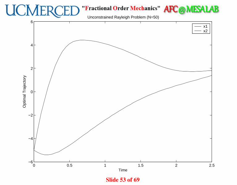
0 0.5 1 1.5 2 2.5−6
−4
−2
0
2
4
6
Time
Opt
imal
Tra
ject
ory
Unconstrained Rayleigh Problem (N=50)
x1x2
Slide 53 of 69

Rayleigh Problem Demo: (please be patient . . . )
Slide 54 of 69

Example 2: Bang problemJ(u) = T
Subject to:x1 = x2, x1(0) = 0, x1(T ) = 300,x2 = u, x2(0) = 0, x2(T ) = 0
Slide 55 of 69

Transcription for free final time problemFree final time problems can be transcribed into fixed final time problems by aug-menting the system dynamics with two additional states (one additional state forautonomous problems). The idea is to specify a nominal time interval, [a, b], forthe problem and to use a scale factor, adjustable by the optimization procedure, toscale the system dynamics and hence, in effect, scale the duration of the time inter-val. This scale factor, and the scaled time, are represented by the extra states. ThenRIOTS can minimize over the initial value of the extra states to adjust the scaling.
Slide 56 of 69

minu,T
g(T, x(T )) +
∫ a+T
a
l(t, x, u)dt
Subject to:x = h(t, x, u) x(a) = ζ , t ∈ [a, a + T ],
where x = [x0, x1, . . . , xn−1]T .
With two extra augmented states [xn, xn+1], we have the new state variable y =[xT , xn, xn+1]
T . Now the original problem can be converted into the equivalent fixedfinal time optimal control problem.
Slide 57 of 69

minu,xn+1
g((b− a)xn+1, x(b)) +
∫ b
a
l(xn, x, u)dt
Subject to:
y =
xn+1h(xn, x, u)xn+1
0
, y(a) =
x(a)aξ
, t ∈ [a, b],
where ξ is the initial value chosen by the user.For autonomous systems, the extra variable xn is not needed because it is not shownexplicitly anywhere.
Slide 58 of 69

sys init.mfunction neq = sys_init(params)% Here is a list of the different system information paramters.% neq = 1 : number of state variables.% neq = 2 : number of inputs.% neq = 3 : number of parameters.% neq = 4 : reserved.% neq = 5 : reserved.% neq = 6 : number of objective functions.% neq = 7 : number of nonlinear trajectory constraints.% neq = 8 : number of linear trajectory constraints.% neq = 9 : number of nonlinear endpoint inequality constraints.% neq = 10 : number of linear endpoint inequality constraints.% neq = 11 : number of nonlinear endpoint equality constraints.% neq = 12 : number of linear endpoint equality constraints.% neq = 13 : 0 => nonlinear, 1 => linear, 2 => LTI, 3 => LQR, 4 => LQR and LTI.% The default value is 0 for all except neq = 6 which defaults to 1.neq = [1 3 ; 2 1 ; 12 2]; % nstates = 3 ; ninputs = 1; 3 endpoint constr.
Slide 59 of 69
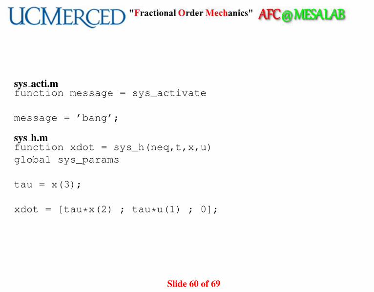
sys acti.mfunction message = sys_activate
message = ’bang’;
sys h.mfunction xdot = sys_h(neq,t,x,u)global sys_params
tau = x(3);
xdot = [tau*x(2) ; tau*u(1) ; 0];
Slide 60 of 69

sys l.mfunction z = l(neq,t,x,u)global sys_paramsz = 0;
sys g.mfunction J = sys_g(neq,t,x0,xf)global sys_paramsF_NUM = neq(5);if F_NUM == 1
J = x0(3);elseif F_NUM == 2
J = xf(1)/300.0 - 1;elseif F_NUM == 3
J = xf(2);end
Slide 61 of 69

sys Dh.mfunction [h_x,h_u] = sys_Dh(neq,t,x,u)global sys_params% h_x must be an n by n matrix.% h_u must be an n by m matrix.
tau = x(3);h_x = zeros(3,3);h_u = zeros(3,1);
h_x(1,2) = tau;h_x(1,3) = x(2);h_x(2,3) = u(1);
h_u(2,1) = tau;
Slide 62 of 69

mainrun.mx0 = [0 1 0 0; 0 1 0 0;1 0 .1 10]% The first column is the initial condition with the optimal duraction% set to 1. The zero in the second column will be used to tell% riots() that the third initial condition is a free variable. The% third and fourth columns represent upper and lower bounds on the% initial conditions that are free variables.
N = 20;u0 = zeros(1,N+2-1);t = [0:10/N:10]; % Set up the initial time vector so that
% the intial time interval is [0,10]*1,[u,x,f]=riots(x0,u0,t,-2,1,[],100,2);Tf = x(3,1)% The solution for the time interval is t*Tf = [0,10]*Tf. Thus, the% solution for the final time is 10*Tf = 29.9813. The actual solution% for the final time is 30.sp_plot(t*Tf,u)xlabel(’Time’),ylabel(’Optimal Control’)figureplot(t*Tf,x)
Slide 63 of 69

0 5 10 15 20 25 30−2.5
−2
−1.5
−1
−0.5
0
0.5
1
1.5
Time
u
Slide 64 of 69

0 5 10 15 20 25 300
50
100
150
200
250
300
350
Time
x
Slide 65 of 69

Bang problem demo: (please be patient . . . )
Slide 66 of 69

References:Adam L. Schwartz, Theory and Implementation of Numerical Methods Based onRunge-Kutta Integration for Solving Optimal Control Problems, Ph.D. Dissertation,University of California at Berkeley, 1996
YangQuan Chen and Adam L. Schwartz.“RIOTS 95 – a MATLAB Toolbox forSolving General Optimal Control Problems and Its Applications to Chemical Pro-cesses,” Chapter in “Recent Developments in Optimization and Optimal Control inChemical Engineering”, Rein Luus Editor, Transworld Research Publishers, 2002.http://www.csois.usu.edu/publications/pdf/pub077.pdf[See also http://www.optimization-online.org/DB HTML/2002/11/567.html]
Slide 67 of 69

Thank you for your attention!Question/Answer Session.
Mobile Actuator and Sensor Networks (MAS-net):http://mechatronics.ece.usu.edu/mas-net/
Task-Oriented Mobile Actuator and Sensor Networks (TOMAS-net)IEEE IROS’05 Tutorial, Edmonton, Canada, August 2, 2005:
http://www.csois.usu.edu/people/yqchen/tomasnet/
RIOTS 95 web:http://www.csois.usu.edu/ilc/riots
Slide 68 of 69
Credits:Dr. Adam L. Schwartz, the father of RIOTS for creating the first Unix OS4 versionof RIOTS. Dr. YangQuan Chen for making the Windows version of RIOTS 95. Dr.Jinsong Liang for making Windows-based RIOTS MEX-6 compatible and versionsfor Linux and Solaris, AIX.
RIOTS 95 users world-wide for feedback.
This set of slides were mostly prepared by Jinsong Liang under the supervision ofProf. YangQuan Chen as a module in Dr. Chen’s ECE/MAE7360 “Robust andOptimal Control” course syllabus. This OCP/RIOTS module has been offered twice(2003, 2004).
Slide 69 of 69