Embed Size (px)
Citation preview

Noname manuscript No.(will be inserted by the editor)
Compact Representation of Near-OptimalInteger Programming Solutions
Thiago Serra · J. N. Hooker
May 2017
Abstract It is often useful in practice to explore near-optimal solutions ofan integer programming problem. We show how all solutions within a giventolerance of the optimal value can be efficiently and compactly represented ina weighted decision diagram, once the optimal value is known. The structure ofa decision diagram facilitates rapid processing of a wide range of queries aboutthe near-optimal solution space. To obtain a more compact diagram, we exploitthe property that such diagrams may become paradoxically smaller when theycontain more solutions. We use sound decision diagrams, which innocuouslyadmit some solutions that are worse than near-optimal. We describe a simple“sound reduction” operation that, when applied repeatedly in any order, yieldsa smallest possible sound diagram for a given problem instance. We find thatsound reduction yields a structure that is typically far smaller than a tree thatrepresents the same set of near-optimal solutions.
Keywords decision diagrams · integer programming · postoptimality
1 Introduction
An integer programming model contains a wealth of information about thephenomenon it represents. An optimal solution of the model, or even a setof optimal solutions, captures only a small portion of this information. Inmany applications, it is useful to probe the model more deeply to explorealternative solutions, particularly solutions that are suboptimal as measuredby the objective function but attractive for other reasons.
Thiago SerraCarnegie Mellon University, Pittsburgh, USAE-mail: [email protected]
J. N. HookerCarnegie Mellon University, Pittsburgh, USAE-mail: [email protected]

2 Thiago Serra, J. N. Hooker
For example, in a recent study [7] an integer programming (IP) model wasformulated to relocate distribution centers across Europe. In the absence ofreliable estimates for fixed costs, the client opted for a suboptimal solution thatrelocated one rather than three distribution centers for only a 0.4% increaseover the optimal cost. One may also wish to know which decisions are invariantacross all near-optimal solutions. This was a key question in a nature reserveplanning study [4] that sought to identify areas that are critical to protectnative species. In addition, there are applications that require the solutionof minor variations of a problem. In some combinatorial auctions [14], forexample, a winners determination problem is first solved to maximize the sumof winning bids, and then re-solved with each winner removed by fixing certainvariables to zero.
In general, one may wish to know which solutions are optimal or near-optimal when certain variables are fixed to desired values, or which values agiven variable can take without sacrificing near-optimality. One may also wishto determine how much a cost coefficient can be perturbed without changingthe optimal cost more than a certain amount.
These questions can be answered if the space of near-optimal solutions iscompactly represented in a transparent data structure; that is, a data structurethat can be efficiently queried to find near-optimal (or optimal) solutions thatsatisfy desired properties. In fact, the task of solving an IP model can be moregenerally conceived as the process of transforming an opaque data structureto a transparent data structure. The constraint set and objective functioncomprise an opaque structure that defines the problem but does not make goodsolutions apparent. A conventional solver transforms the problem statementinto a very simple transparent structure: an explicit list of one or more optimalsolutions. The ideal would be to derive a more general data structure thatcompactly but transparently represents the space of near-optimal solutionsand how they relate to each other.
We propose a weighted decision diagram for this purpose. Binary andmultivalued decision diagrams have long been used for circuit design, formalverification, and other purposes [2,6,21,24,28], but they can also compactlyrepresent solutions of a discrete optimization problem [3,5,16,19]. A weighteddecision diagram represents the objective function values as well. Such adiagram can be built to represent only near-optimal solutions, and it cancan be easily queried for solutions that satisfy desired properties. This isbecause solutions correspond straightforwardly to paths in the diagram, andtheir objective function values to the length of the paths.
A simple example illustrates the idea. The IP problem
minimize 4x1 + 3x2 + 2x3subject to x1 + x3 ≥ 1, x2 + x3 ≥ 1, x1 + x2 + x3 ≤ 2
x1, x2, x3 ∈ {0, 1}(1)
has optimal value 2. The branching tree of Fig. 1(a) represents the three feasi-ble solutions that have a value within 4 of the optimum, namely (x1, x2, x3) =(1, 0, 1), (0, 1, 1), (0, 0, 1). A dashed arc represents setting xj = 0, and a solid

Compact Representation of Near-Optimal Integer Programming Solutions 3
(a)
x1 tr.....................................................................................................................................................
..........................
..........................
...........x2 t.......................................
t........................................................................................................................
..........................
....................x3 t............................................................................
t............................................................................t............................................................................t t t
(b)
tr........................................................................................................................................ 4.............
..........................
..........................
...........t..........................
..........................
......................
t............................................................................................................................................................3
............. ............. ..........................................................
t............................................................................2 tt
(c)
tr............................................................................................4
.......................................
.............t............................................................................................3
.......................................
.............t............................................................................2 tt
Fig. 1: (a) Branching tree for near-optimal solutions of (1). (b) Reduced weighted decisiondiagram representing the same solutions. (c) Sound decision diagram for (1).
arc represents setting xj = 1. Figure 1(b) is a decision diagram that representsthe same solutions. The solid arcs are assigned weights (lengths) equal to thecorresponding objective function coefficients, while the dashed arcs have lengthzero. Each path from the root r to the terminus t represents a feasible solutionwith cost at most 6, where the cost of the solution is the length of the path.The decision diagram is reduced, meaning that it is the smallest diagram thatrepresents this set of solutions. It is well known that, for a given ordering ofthe variables, there is a unique reduced diagram representing a given set ofsolutions [6].
Although reduced decision diagrams tend to provide a much more compactrepresentation than a branching tree, they can nonetheless grow rapidly. Toaddress this issue, we take advantage of the fact that modifying a diagram torepresent a larger solution set can, paradoxically, result in a smaller diagram.We adopt the concept of a sound decision diagram, introduced by [18], which isa diagram that represents all near-optimal solutions along with some spurioussolutions whose objective function values are worse than near-optimal. Thespurious solutions may be feasible or infeasible. By judiciously admittingspurious solutions into the diagram, one can significantly reduce its size whilemaintaining soundness of the near-optimal solution set.
In particular, we show that a certain sound reduction operation, whichreplaces a pair of nodes with a single node, yields a smaller sound diagram.Our main theoretical result is that repeated application of sound reductionoperations, in any order, results in a smallest possible sound diagram for agiven problem and variable ordering. It is smallest in the sense that it has aminimum number of arcs and a minimum number of nodes. We call such adiagram sound reduced. A problem may have multiple sound-reduced diagrams,but they all have the same minimum size.
Sound diagrams have several advantages for postoptimality analysis. Asidefrom their smaller size, they allow for easy extraction of near-optimal solutions.One need only to enumerate paths in the diagram while discarding those thatrepresent spurious solutions, which are easily identified by the fact that theirvalues are too far from the optimum. In order to infer that solutions are
4 Thiago Serra, J. N. Hooker
spurious while constructing and when querying such diagrams, the optimalvalue is first obtained by solving the problem with a conventional solver.
For example, Fig. 1(c) illustrates a sound diagram for problem (1). Itrepresents the three solutions within 4 of the optimal value, plus a spurioussolution (x1, x2, x3) = (1, 1, 1) that is discarded because its value is greaterthan 6. This solution happens to be infeasible, but it is not necessary to checkfeasibility, which is time-consuming. It is only necessary to compute the pathlength.
A further advantage of sound diagrams is that the presence of spurioussolutions has no effect whatever on the implementation or complexity of manytypes of postoptimality analysis. It is enough that the diagram represent allnear-optimal solutions.
We begin below with a review of related work, followed by four sections thatdevelop the underlying theory of sound diagrams. Section 3 introduces somebasic concepts and properties of decision diagrams. Section 4 develops the ideaof soundness and shows that it is a useful concept only when suboptimal (aswell as optimal) solutions are represented. Section 5 proves the main resultthat sound reduction yields a sound diagram of minimum size. It also showsby counterexample that there need not be a unique sound-reduced diagramfor a given problem. Section 6 explains why it is not practical to admitsuperoptimal solutions into sound diagrams, even though this may result insmaller diagrams.
The remaining sections apply the theory of sound diagrams to integerprogramming. Section 7 presents an algorithm that constructs a sound diagramfor a given integer programming problem, assuming that the optimal value hasbeen obtained by solving the problem with a conventional solver. Section 8shows how to introduce sound reduction into the algorithm, thereby obtaininga smallest possible sound diagram for the problem. Section 9 then describesseveral types of postoptimality analysis that can efficiently be performed ona sound diagram. Section 10 reports computational tests that measure howcompactly sound diagrams can represent near-optimal solutions, and the timerequired to compute the diagrams. Based on instances from MIPLIB, it isfound that decision diagrams represent near-optimal solutions much morecompactly than a branching tree, and that in most instances, sound reductionsubstantially reduces the size of the diagrams. The paper concludes with asummary and agenda for future research.
2 Related Work
To our knowledge, no previous study addresses the issue of how to representnear-optimal solutions of IP problems in a compact and transparent fashion. Afew papers have proposed methods for generating multiple solutions. Scattersearch is used in [13] to generate a set of diverse optimal and near-optimalsolutions of mixed integer programming (MIP) problems. However, since itis a heuristic method, it does not obtain an exhaustive set of solutions for

Compact Representation of Near-Optimal Integer Programming Solutions 5
any given optimality tolerance. Diverse solutions of an MIP problem havealso been obtained by solving a sequence of MIP models, beginning with thegiven problem, in which each seeks a solution different from the previous ones.This approach is investigated in [15], where it is compared with solving amuch larger model that obtains multiple solutions simultaneously. However,neither method is scalable, as there may be a very large number of near-optimalsolutions.
The “one-tree” method of [8] generates a collection of optimal or near-optimal solutions of a mixed-integer programming problem by extending abranching tree that is used to solve the problem. While possible, the collectionis not intended to be exhaustive, and there is no indication of how to representthe collection compactly or query more easily. A “branch-and-count” methodis presented in [1] for generating all feasible solutions of an IP problem, basedon the identification of “unrestricted subtrees” of the branching tree. These aresubtrees in which all values of the unfixed variables are feasible. We use a sim-ilar device as part of our mechanism for constructing sound decision diagrams.However, we focus on compact representation of near-optimal solutions.
The commercial solver CPLEX has offered a “solution pool” feature sinceversion 11.0 [22] that relies on the one-tree method. The solution pool hasbeen supported by the the GAMS modeling system since version 22.6 [11]. Bycontrast, postoptimality software based on decision diagrams operates apartfrom the solution method, requiring only the optimal value from the solver.It also differs by generating an exhaustive set of near-optimal solutions andorganizing them in a decision diagram that is convenient for postoptimalityanalysis.
Integer programming sensitivity analysis has been investigated for sometime, as for example in [9,10,12,20,23,26,27]. Sound decision diagrams can beused to analyze sensitivity to perturbations in objective coefficients, becausethese appear as arc lengths in the diagram, and we show how to do so. However,our main interest here is in probing the near-optimal solution set that resultsfrom the original problem data.
Decision diagrams were first proposed for IP postoptimality analysis in[17], and the concept of a sound diagram was introduced in [18]. The presentpaper extends this work in several ways. It proves several properties of sounddiagrams, introduces the sound reduction operation, and proves that soundreduction yields a sound diagram of minimum size. It also presents algo-rithms for generating sound-reduced diagrams for IP problems and conductingpostoptimality analysis on these diagrams, as well as reporting computationaltests on the representational efficiency of the diagrams.
3 Decision Diagrams for Discrete Optimization Problems
For our purposes, we associate a decision diagram with a discrete optimizationproblem of the form
min{f(x) | x ∈ S} (P)

6 Thiago Serra, J. N. Hooker
where S ⊆ S1 × . . . × Sn and each variable domain Sj is finite. A decisiondiagram associated with (P) is a multigraph D = (U,A, `) with the followingproperties:
– The node set U is partitioned U = U1 ∪ · · · ∪ Un+1, where U1 = {r} andUn+1 = {t}. We say r is the root node, t the terminal node, and Uj is layerj of D for each j.
– The arc set A is partitioned A = A1 ∪ · · · ∪ An, where each arc in Ajconnects a node in Uj with a node in Uj+1, for j = 1, . . . , n.
– Each arc a ∈ Aj has a label `(a) ∈ Sj for j = 1, . . . , n, representing a valueassigned to variable xj . The arcs leaving a given node must have distinctlabels.
The labels on each path p of D from r to t represent an assignment to x, whichwe denote x(p). We let Sol(D) denote the set of solutions represented by ther–t paths. We say that D exactly represents S when Sol(D) = S.
A weighted decision diagram associated with (P) is a multigraphD(U,A, `, w)that satisfies the above properties, plus the following:
– Each arc a ∈ A has a weight w(a), such that∑a∈p w(a) = f(x(p)) for
any r–t path p of D. Thus the total weight w(p) of an r–t path p is theobjective function value of the corresponding solution.
A weighted decision diagram associated with problem (P) exactly represents(P) when Sol(D) = S. In this case, the optimal value z∗ of (P) is the weight ofany minimum-weight r–t path of D, and the optimal solutions of (P) are thosecorresponding to minimum-weight r–t paths. From here out, we will refer toa weighted decision diagram simply as a decision diagram, and to a diagramwithout weights as an unweighted decision diagram.
An unweighted decision diagram D is reduced when redundancy is removed.To make this precise, let a suffix of u ∈ Uj be any assignment to xj , . . . , xnrepresented by a u–t path in D, and let Suf(u) be the set of suffixes of u.Then D is reduced when Suf(u) 6= Suf(v) for all u, v ∈ Uj with u 6= v and allj = 1, . . . , n. As noted earlier, for any fixed variable ordering, there is a uniquereduced unweighted decision diagram that exactly represents a given feasibleset S, and this diagram is the smallest one that exactly represents S [6].
Given a path π from a node in layer j to a node in layer k, it will beconvenient to denote by x(π) the assignment to (xj , . . . , xk−1) indicated bythe labels on path π. We also let xi(π) denote the the assignment to xi inparticular, and we let w(π) denote the weight of π. A summary of notationused throughout the paper can be found in Table 1.
The following simple property of decision diagrams will be useful.
Lemma 1 Given any pair of distinct nodes u, v in layer j of a decisiondiagram, let π be an r–u path and ρ an r–v path. Then x(π) 6= x(ρ).
Proof If x(π) = x(ρ), then in particular x1(π) = x1(ρ). This implies that πand ρ lead from r to the same node u in U2, since distinct arcs leaving r musthave distinct labels. Arguing inductively, π and ρ lead from the same node in

Compact Representation of Near-Optimal Integer Programming Solutions 7
Table 1: List of symbols.
r root node of a decision diagramt terminal node of a decision diagramUj set of nodes in layer j of a diagramAj set of arcs connecting nodes in Uj with nodes in Uj+1
`(a) label of arc a, representing value of xj if a ∈ Ajw(a) weight (cost, length) of arc ax(p) assignment to x represented by r–t path pw(p) weight of r–t path px(π) assignment to xj , . . . , xk−1 represented by u–v path π (u ∈ Uj , v∈ Uk)xi(π) assignment to xi represented by π, where j ≤ i < kw(π) weight of path πw(u, u′) weight of minimum-weight path from node u to node u′
Sol(D) set of solutions represented by r–t paths in diagram Dz∗ optimal value of problem (P)P(∆) problem of finding ∆-optimal solutions of (P)S(∆) set of ∆-optimal solutions of (P)ILP(∆) problem of finding ∆-optimal solutions of (ILP)Pre(u) set of prefixes of node uSuf(u) set of suffixes of node uSuf∆(u) set of ∆-suffices of node u of a diagram D; i.e., set of suffixes of u
that are part of some ∆-optimal solution represented by Dlhs.u left-hand-side state at node uLCDSj [u, v] weight of least-cost differing suffix when reducing u into vW maximum width of (number of nodes in) layers of a diagramSmax size of largest variable domain
Uk to the same node in Uk+1 for k = 1, . . . , j − 1. This implies that u = v,contrary to hypothesis. �
4 Sound Decision Diagrams
We are interested in constructing decision diagrams that represent near-optimalsolutions of (P). Let x be a ∆-optimal solution of (P) when x ∈ S andf(x) ≤ z∗+∆, for ∆ ≥ 0. We denote by S(∆) is the set of ∆-optimal solutionsof (P), so that S(0) is the set of optimal solutions. We let P(∆) denote thethe problem of finding ∆-optimal solutions of (P).
We say that D exactly represents P(∆) when Sol(D) = S(∆). Since such adecision diagram can be quite large, we wish to identify smaller diagrams thatapproximately represent P(∆). We therefore study decision diagrams that aresound for P(∆), which represent a superset of S(∆). Specifically, D is soundwhen
S(∆) = Sol(D) ∩ {x ∈ S1 × · · · × Sn | f(x) ≤ z∗ +∆}Thus a sound diagram can represent, in addition to ∆-optimal solutions,feasible and infeasible solutions that are worse than ∆-optimal. We referto these as spurious solutions. A proper sound diagram represents a propersuperset of the ∆-optimal solutions and therefore represents some spurioussolutions.

8 Thiago Serra, J. N. Hooker
We prefer a sound diagram D that is minimal for P(∆), meaning thatevery node of D, and every arc of D, lies on some r–t path that represents asolution in S(∆). If a sound diagram is not minimal, nodes and/or arcs can beremoved without destroying soundness. Since their removal does not enlargethe set represented by the diagram, we obtain a smaller diagram that is anequally accurate approximation of S(∆).
It is easy to check whether a node or arc can be removed while preservingsoundness. For any two nodes u, u′ in different layers of D, let w(u, u′) be theweight of a minimum-weight path from u to u′ (infinite if there is no path).Then node u can be removed if and only if
w(r, u) + w(u, t) > z∗ +∆
An arc a connecting u ∈ Uj with u′ ∈ Uj+1 can be removed if and only if
w(r, u) + w(a) + w(u′, t) > z∗ +∆ (2)
Interestingly, a proper sound diagram for P(0) is never minimal. Thisimplies that there is no point in considering sound diagrams to represent theset of optimal solutions. They are useful only for representing sets of near-optimal solutions.
Theorem 1 No proper sound decision diagram is minimal for P(0).
Proof Suppose to the contrary that diagram D is a minimal for P(0) andcontains a suboptimal r–t path p. For any given node u in p, let π(u) be theportion of p from r to u. Select a node u∗ in p that maximizes the numberof arcs in π(u∗) subject to the condition that π(u∗) is part of some optimal(minimum-weight) r–t path in D (Fig. 2). We note that u∗ 6∈ Un+1, sinceotherwise p would be an optimal r–t path. Thus p contains an arc a from u∗
to some node u′. Furthermore, u∗ 6∈ U1 since otherwise arc a would prevent Dfrom being minimal. Now since D is minimal, arc a belongs to some optimalr–t path, which we may suppose consists of π′, a, and σ′. Hence, π(u∗) andπ′ are both optimal r–u∗ paths, and thus the r–t path consisting of π(u′) andσ′ is also optimal. This implies that π(u′), which contains one more arc thanπ(u∗), is part of an optimal r–t path, contrary to the definition of u∗. �
The following property of sound diagrams is easily verified.
Lemma 2 If a decision diagram D is sound for P(∆), then D is sound forP(δ) for any δ ∈ [0, ∆].
Thus the set of sound decision diagrams of P(∆) is a subset of that of P(δ)for any δ ∈ [0, ∆].
Corollary 1 The size of a smallest sound diagram for P(∆), as measured bythe number of arcs or the number of nodes, is monotone nondecreasing in ∆.

Compact Representation of Near-Optimal Integer Programming Solutions 9
π(u∗) π ′
a
σ ′
tr.............................................................................................................................................................................................................................................................................................................
.............................................................................................................................................................................................................................................................................................................tu∗............................................................................t u′..................................................................................................................................................................................................................................tt
Fig. 2: Illustration of the proof of Theorem 1.
5 Sound Reduction
Sound reduction is a tool for reducing the size of a given sound diagram, gen-erally at the cost of increasing the number of spurious solutions it represents.Given distinct nodes u, v ∈ Uj for 1 < j ≤ n, we can sound-reduce u into vwhen diverting to v the arcs coming into u, and deleting u from the diagram,removes no ∆-optimal solutions and adds only spurious solutions. Thus soundreduction removes at least one node without destroying soundness. In fact, wewill see that repeated sound reduction yields the smallest sound diagram fora given ∆.
Let a ∆-suffix of node u ∈ Uj be any suffix in Suf(u) that is part of a∆-optimal solution, and let Suf∆(u) be the set of ∆ suffixes of u. Also let aprefix of u be any assignment to (x1, . . . , xj−1) represented by an r–u path,and let Pre(u) be the set of prefixes of u. Then u can be sound-reduced into vif:
Suf∆(u) ⊆ Suf(v) (3)
w(π) + w(σ) > z∗ +∆ when x(π) ∈ Pre(u) and x(σ) ∈ Suf(v) \ Suf(u) (4)
Sound reduction is accomplished as follows. For every arc a from some nodeq ∈ Uj−1 to u, remove a and create an arc from q to v with label `(a) andweight w(a). Then remove u and any successor of u that is disconnected fromr. That is, remove u and any successor u′ of u for which all r–u′ paths in Dcontain u.
Condition (3) ensures that any ∆-optimal solution whose r–t path passesthrough u remains in the diagram after sound reduction, with the same cost.

10 Thiago Serra, J. N. Hooker
Condition (4) ensures that only spurious solutions are added to the diagram.So we have,
Theorem 2 Sound reduction preserves soundness.
Figure 3 illustrates sound reduction. Figure 3(a) is a reduced diagram thatis sound for a problem P(∆) with z∗ = 2 and ∆ = 6. Dashed arcs have label0 and weight 0, and solid arcs have label 1 and weights as shown. Figure 3(b)shows the result of sound-reducing node u1 into node v1. Condition (3) issatisfied because Suf∆(u1) = {(1, 1, 0, 0)} ⊆ {(1, 1, 0, 0), (1, 1, 0, 1)} = Suf(v1).Condition (4) is satisfied because Pre(u1) = {(1, 1)}, Suf(v1) \ Suf(u1) ={(1, 1, 0, 1)}, and the solution (x1, . . . , x6) = (1, 1, 1, 1, 0, 1) has cost 9 > z∗+∆.We could have also reduced u2 into v2, u3 into v3, or u3 into q.
A sound diagram for P(∆) is sound-reduced if no further sound reductionsare possible. We can show that a minimal sound-reduced diagram is thesmallest diagram that is sound for P(∆). For example, the diagram in Fig. 3(b)is sound-reduced, and it is in fact the smallest sound diagram for P(∆) with∆ = 6. Establishing this result requires two lemmas.
Lemma 3 Given a sound-reduced diagram D for P(∆), any two distinct nodesu, v ∈ Uj of D satisfy Suf∆(u) 6= Suf∆(v).
Proof Suppose to the contrary that Suf∆(u) = Suf∆(v), and assume withoutloss of generality that w(r, u) ≥ w(r, v). We will show that u can be sound-reduced into v, contrary to hypothesis. Condition (3) for sound reduction isobviously satisfied. Also condition (4) is satisfied, because if x(π) ∈ Pre(u) andx(σ) ∈ Suf(v) \ Suf(u), then x(σ) 6∈ Suf∆(u), and therefore x(σ) 6∈ Suf∆(v).This implies w(r, v) + w(σ) > z∗ + ∆. But w(π) + w(σ) ≥ w(r, u) + w(σ) ≥w(r, v) + w(σ), and (4) follows. �
(a)
x1 tr..........................
..........................
........................
........................................................................................................................................
4
x2 t............................................................................ 1
t........................................................................................................... 1.............
..........................
....................x3 t............................................................................ 1
tu1............................................................................
1
t v1............................................................................
1x4 t.............
.............
.............
tu2............................................................................
1
t v2............................................................................
1x5 tq
2.......................................................................................................................................................................................
..........................
.......................... ............. ............. ............. ...........
tu3.......................................
t v3.......................................x6 t.............
.............
.............
t2
..........................................................................................................................................................................................
..............................................................................
.....................
tt
(b)
tr..........................
..........................
........................
........................................................................................................................................
4t............................................................................ 1 1t............................................................................................................................................................................
............. ............. ........t............................................................................ 1
t v1............................................................................
1t.......................................
t v2............................................................................
1tq2
.......................................................................................................................................................................................
..........................
.......................... ............. ............. ............. ...........
t v3.......................................t.............
.............
.............
t2
..........................................................................................................................................................................................
..............................................................................
.....................
tt
Fig. 3: Reduced (a) and sound-reduced (b) decision diagrams for z∗ = 2 and ∆ = 6.

Compact Representation of Near-Optimal Integer Programming Solutions 11
D
tr............................................................................................................................................................................................................................................................π
π
.....................................................................................................................................................................................................................................................................................................................................................
............................................................................................................................................................................................................................................................
ρ
tu ............................................................................................................................................................................................................................................................
τ
t v............................................................................................................................................................................................................................................................
τ
σ
.....................................................................................................................................................................................................................................................................................................................................................tt
’
D′
tr
π ′
.............................................................................................................................................................................................................................................................................................................
ρ ′
.............................................................................................................................................................................................................................................................................................................tu′
τ ′
..................................................................................................................................................................................................................................................................................................................................................................
..................................................................................................................................................................................................................................
σ ′ σ ′
..................................................................................................................................................................................................................................................................................................................................................................tt
Fig. 4: Illustration of the proof of Lemma 4.
Lemma 4 Let D be a minimal sound-reduced diagram for P(∆). For anynode u in layer j of D, and any other diagram D′ with the same variableordering that is sound for P(∆), there is a node u′ in layer j of D′ withSuf∆(u) = Suf∆(u′).
Proof Suppose to the contrary that there is a node u in layer j of D, and somesound diagram D′ in which layer j contains no node with the same ∆-suffixesas u. We will show that D must then contain a node v into which u can besound-reduced, contrary to hypothesis.
Let π be a minimum-weight r–u path in D. Since D is minimal, nodeu belongs to some path that represents a ∆-optimal solution. So since π is aminimum-weight r–u path, x(π) is the prefix of some ∆-optimal solution. Thussince D′ is sound for P(∆), layer j of D′ must contain a node u′ and an r–u′
path π′ with x(π′) = x(π). Since every ∆-optimal solution represented by D isalso represented by D′, we have that Suf∆(u) ⊆ Suf∆(u′), due to the fact thatπ is a minimum-weight path. However, by hypothesis Suf∆(u) 6= Suf∆(u′),and so we have Suf∆(u′) \ Suf∆(u) 6= ∅.
Now consider any u′–t path σ′ for which x(σ′) ∈ Suf∆(u′) \ Suf∆(u). Thisimplies that x(σ′) is the suffix of some ∆-optimal solution, and so there mustbe an r–u′ path ρ′ with
w(ρ′) + w(σ′) ≤ z∗ +∆ (5)
However, we can see as follows that (x(π′), x(σ′)) is not a ∆-optimal solution.Note that by Lemma 1, π is the only path in D representing x(π) = x(π′).Thus if (x(π′), x(σ′)) were ∆-optimal, the soundness of D would imply thatx(σ′) = x(σ) ∈ Suf∆(u) for some u–t path σ, which contradicts the fact that

12 Thiago Serra, J. N. Hooker
x(σ′) ∈ Suf∆(u′) \ Suf∆(u). So (x(π′), x(σ′)) is not ∆-optimal, which meansw(π′) + w(σ′) > z∗ + ∆. This and (5) imply w(ρ′) < w(π′). But (5) alsoimplies that the sound diagram D must contain a node v and an r–v path ρwith x(ρ′) = x(ρ), so that w(ρ) < w(π). Since π is a minimum-weight r–upath, this implies u 6= v.
We now show that u can be sound-reduced into v by verifying conditions(3) and (4). To show (3), consider any u–t path τ with x(τ) ∈ Suf∆(u). Sinceπ is a minimum-weight r–u path, (x(π), x(τ)) is a ∆-optimal solution. Nowsince D′ is sound for P(∆) and x(π) = x(π′), there is a u′–t path τ ′ in D′
for which (x(π′), x(τ ′)) is ∆-optimal. This means (x(ρ′), x(τ ′)) is ∆-optimalbecause w(ρ′) < w(π′), which implies that (x(ρ), x(τ)) is ∆-optimal. Since byLemma 1, ρ is the only path representing x(ρ), there must be a v–t path τwith x(τ) = x(τ) and x(τ) ∈ Suf∆(v). This implies x(τ) ∈ Suf(v) and (3).
Finally, to show (4), let π be an r–u path with x(π) ∈ Pre(u), and let σ bea v–t path with x(σ) ∈ Suf(v)\Suf(u). Note that if w(ρ)+w(σ) > z∗+∆, thensince w(π) ≥ w(π) > w(ρ), we have w(π)+w(σ) > z∗+∆, and (4) follows. Wemay therefore suppose w(ρ) + w(σ) ≤ z∗ +∆, which means that (x(ρ), x(σ))is ∆-optimal because D is sound. Since D′ is sound and x(ρ) = x(ρ′), byLemma 1 there must be a u′–t path σ′ for which x(σ′) = x(σ) and (x(ρ′), x(σ′))is ∆-optimal. This means that D′ represents the solution (x(π′), x(σ′)), whichis the same as (x(π), x(σ)). But since x(σ) 6∈ Suf(u), D does not representthe solution (x(π), x(σ)), which therefore cannot be ∆-optimal. Thus since D′
represents this solution, it must be spurious, and we have w(π)+w(σ) > z∗+∆.This implies w(π) + w(σ) > z∗ +∆ and (4). �
Theorem 3 A sound decision diagram D for P(∆) has a minimum numberof nodes and a minimum number of arcs, among diagrams that are sound forP(∆) and have the same variable ordering, if and only if D is minimal andsound-reduced.
Proof If D is not minimal, we can remove one or more nodes or arcs, and ifD is not sound-reduced, we can remove at least one node. Thus D is minimaland sound-reduced if it has a minimum number of nodes and arcs.
To prove the converse, suppose D is minimal and sound-reduced. Due toLemma 3, all nodes in any given layer j of D have sets of ∆-suffixes. ByLemma 4, these distinct sets of ∆-suffixes exist for nodes in layer j of anysound diagram for P(∆). Thus any sound diagram for P(∆) has at least asmany nodes as D. Furthermore, the minimality of D implies that any arc aleaving a node u in layer j of D is part of some ∆-optimal solution. Givenany diagram D′ that is sound for P(∆), the node u′ in layer j of D′ withSuf∆(u′) = Suf∆(u) must have an outgoing arc with the same label as a.Thus D′ has at least as many arcs as D. �
Although all sound-reduced diagrams for a given P(∆) have minimum size,they are not necessarily identical. For example, while all sequences of soundreductions of Fig. 3(a) terminate in the same diagram Fig. 3(b), this is notthe case for the slightly different diagram of Fig. 5(a). Sound-reducing u3 into

Compact Representation of Near-Optimal Integer Programming Solutions 13
(a)
tr..........................
..........................
........................
........................................................................................................................................
4t............................................................................ 1
t........................................................................................................... 1.............
..........................
....................t............................................................................ 1
tu1............................................................................
1
t v1............................................................................
1t.......................................
tu2............................................................................
1
t v2.......................................tq
2.......................................................................................................................................................................................
..........................
.......................... ............. ............. ............. ...........
tu3.......................................
t v3.......................................t.............
.............
.............
t2
..........................................................................................................................................................................................
..............................................................................
.....................
tt
(b)
tr..........................
..........................
........................
........................................................................................................................................
4t............................................................................ 1
t........................................................................................................... 1.............
..........................
....................t............................................................................ 1
tu1............................................................................
1
t v1............................................................................
1t.......................................
tu2........................................................................................................................................................................
1t v2.......................................tq
2.......................................................................................................................................................................................
..........................
.......................... ............. ............. ............. ...........
t v3.......................................t.............
.............
.............
t2
..........................................................................................................................................................................................
..............................................................................
.....................
tt
(c)
tr..........................
..........................
........................
........................................................................................................................................
4t............................................................................ 1
t........................................................................................................... 1.............
..........................
....................t............................................................................ 1
tu1............................................................................
1
t v1............................................................................
1t.......................................
tu2........................................................................................................................................................................1
t v2.......................................tq
2.......................................................................................................................................................................................
..........................
.......................... ............. ............. ............. ...........
t v3.......................................t.............
.............
.............
t2
..........................................................................................................................................................................................
..............................................................................
.....................
tt
Fig. 5: Distinct sound-reduced diagrams (b) and (c) obtained from diagram (a), where z∗ = 2and ∆ = 6.
q yields the sound-reduced diagram of Fig. 5(b), and sound-reducing u3 intov3 yields Fig. 5(c). Both diagrams are of minimum size and satisfy Lemma 4,but they are distinct.
6 Two-Sided Soundness
A sound diagram is permitted to represent feasible and infeasible solutionsthat are worse than ∆-optimal. A natural question is whether it would beuseful to allow (infeasible) solutions that are better than optimal. Superoptimalsolutions, like solutions that are worse than ∆-optimal, can be filtered outduring postoptimality analysis by examining only objective function values.
Since such a diagram D requires excluding solutions with values on eitherside of the interval [z∗, z∗ + ∆], we will say that it has two-sided soundness,meaning that it satisfies
S(∆) = Sol(D) ∩ {x ∈ S1 × · · · × Sn | z∗ ≤ f(x) ≤ z∗ +∆}
Conceivably, this weaker condition for including solutions could allow moreflexibility for finding a small sound diagram.
There is a theoretical reason, however, that two-sided soundness is lesssuitable for practical application. In a one-sided sound diagram, it is easy tocheck whether a given r–u path of cost w can be completed to represent aδ-optimal solution. Namely, find a shortest u–t path and check whether itslength is at most z∗ − w + δ. In a two-sided sound diagram, this decisionproblem is NP-complete. It is therefore difficult to extract δ-optimal solutionsfrom a two-sided sound diagram.
Theorem 4 Checking whether some r–t path in a given decision diagram hascost that lies in an given interval [z∗, z∗ + δ] is NP-complete.

14 Thiago Serra, J. N. Hooker
Proof The problem belongs to NP because an r–t path with cost in [z∗, z∗+δ]is a polynomial-size certificate. It is NP-complete because we can reduce thesubset sum problem to it. Given a set S = {s1, . . . , sn} of integers, the subsetsum problem is to determine whether some nonempty subset of these integerssums to zero. We can solve the problem by constructing a decision diagram asfollows. Let U1 = {r}, Uj = {uj1, . . . , ujn} for j = 2, . . . , n, and Un+1 = {t}.There is one arc with weight sk from r to each u2k, k = 1, . . . , n. There aretwo arcs from each ujk to uj+1,k for j = 2, . . . , n−1, one with weight zero, andthe other with weight sj if j−1 < k and weight sj+1 otherwise. There are twoarcs from each unk to t, one with weight zero, and the other with weight sn−1if k = n and weight sn otherwise. Then there is a one-to-one correspondencebetween r–t paths and nonempty subsets of S. The subset sum problem hasa solution if and only if there is an r–t path with cost in the interval [0, 0]. �
Corollary 2 Checking whether a given r–u path can be extended to a pathwith cost in [z∗, z∗ + δ] is NP-complete.
Proof Let the given r–u path in diagram D have cost w, and consider thedecision diagram D′ consisting of all u–t paths of D. The path extensionproblem is equivalent to checking whether some u–t path in D′ has cost in theinterval [z∗−w, z∗−w+ δ], which by Theorem 4 is an NP-complete problem.�
7 Sound Diagrams for Bounded Integer Linear Programs
We now specialize problem (P) to an integer linear program:
min{cx | Ax ≥ b, x ∈ S1 × . . .× Sn} (ILP)
in which A is an m × n matrix and each Sj is a finite set of integers. Wewish to build a sound decision diagram that represents ∆-optimal solutions of(ILP); that is, a sound diagram for ILP(∆). We assume that (ILP) has beensolved to optimality and the optimal value z∗ is known. This will acceleratethe construction of a sound diagram.
We build the diagram by constructing a branching tree, identifying nodesthat necessarily have the same set of ∆-suffixes, and removing some nodesthat cannot be part of a ∆-optimal solution. To accomplish this, we associatewith every node u ∈ Uj a state (u.lhs, w(r, u)). In the simplest case, u.lhs is anm-tuple in which component i is the sum of left-hand-side terms of inequalityconstraint i that have been fixed by branching down to layer j. The root noder initially has state (0, 0), where 0 is a tuple of zeros. We can identify nodesu, u′ that have the same lhs state, because they necessarily have the same∆-suffixes. The resulting node v has state (v.lhs, w(r, v)), where v.lhs = u.lhsand w(r, v) = min{w(r, u), w(r, u′)}. Thus the state variable w(r, v) maintainsthe weight of a minimum-weight r–v path in the current diagram.
We can also observe that inequality constraint i is satisfied at node u ∈ Uj ,for any values of xj , . . . , xn, when the sum of the fixed terms on the left-hand

Compact Representation of Near-Optimal Integer Programming Solutions 15
side is sufficiently large. Specifically, inequality i is necessarily satisfied whenthe sum of these terms is at least bi −Mij , where
Mij =
n∑k=j
min{Aikxk | xk ∈ Sk
}This allows us to update the lhs state to min{u.lhs, b −Mj} and still iden-tify nodes that have the same state. Here, Mj = (M1j , . . . ,Mmj), and theminimum is taken componentwise.
We can remove a node u ∈ Uj when the cost of any r–t path through umust be greater than z∗ +∆, based on the linear relaxation of (ILP) at nodeu. We therefore remove u when w(r, u) + LPj(u.lhs) > z∗ +∆, where
LPj(u.lhs) = min{ j−1∑k=1
ckxk
∣∣∣ n∑k=j
Akxk ≥ b− u.lhs, xk ∈ Ik, k = j, . . . , n}
and Ik is the interval [minSk,maxSk]. This can remove some spurious solu-tions, but not necessarily all, because w(r, u) can underestimate the weight ofr–u paths, and LPj(u.lhs) can underestimate the weight of u–t paths.
The diagram construction is controlled by Algorithm 1, which maintainsunexplored nodes in a priority queue that determines where to branch next.When exploring node u ∈ Uj , the procedure invokes Algorithm 2 to create anoutgoing arc for each value in the domain Sj of xj . Some of these arcs maylead to dead-end nodes based the LP relaxation as described above. If all leadto dead ends, u and predecessors of u with no outgoing arcs are removed bythe subroutine at the bottom of Algorithm 1.
Each surviving arc a out of u is processed as follows. Let the node q at theother end of arc a have state (q.lhs, w(r, u) + cj`(a)), where
q.lhs = min{b−Mj , u.lhs +Aj`(a)
}If no node currently in Uj+1 has the same lhs state as q, add node q to Uj+1.Otherwise, some node v ∈ Uj+1 has v.lhs = q.lhs, and we let arc a run from uto v, updating w(r, v) if necessary. If v has been explored already, it is revisitedin Algorithm 3, because the updated value of w(r, v) may affect which nodesand arcs can be deleted.
A key concept in the procedure is that of a closed node. The terminalnode t is designated as closed (t.closed = true) when it is first reached inAlgorithm 2. Higher nodes in the diagram are recursively marked as closedwhen all of their successors are closed. The recursion is implemented by main-taining the number u.openArcs of arcs from node u that do not lead to closednodes. When Algorithm 1 pops u from the priority queue and processes it,u.openArcs is set to the number |Sj | of domain elements of xj . Algorithm 1decrements this number for each dead-end arc, and Algorithm 2 decrementsit for each arc leading to a pre-existing node that is closed. Node u is closedwhen u.openNodes reaches zero.

16 Thiago Serra, J. N. Hooker
Algorithm 1 Builds sound diagram for (ILP) using an arbitrary search type
1: procedure PopulateSoundDiagram()2: r ← new Node(min{0,M1}, 0)3: U1 ← {r}4: PriorityQueue← {(1, r)} . Begins search at root node r5: RevisitBFSQueue← {}6: while PriorityQueue 6= ∅ do7: (j, u)← PriorityQueue.pop() . Queue policy defines search type8: u.openArcs← |Sj |9: Deadend← true
10: for α ∈ Sj do11: Success← TryBranching(j, u, α) . Algorithm 212: Deadend← Deadend ∧ ¬Success13: end for14: if Deadend then . No branch succeeded15: RemoveDeadendNode(j, u) . Procedure below16: else if RevisitBFSQueue 6= ∅ then . Nodes following u reopened17: RevisitNodes() . Algorithm 318: else if u.openArcs = 0 then . Nodes following u are all closed19: CloseNode(j, u) . Algorithm 420: end if21: u.explored← true22: end while23: end procedure
Subroutine: Removes nodes that cannot reach t recursively
24: procedure RemoveDeadendNode(j, u)25: Uj ← Uj \ {u}26: for all a = (v, u) ∈ A do27: A← A \ {a}28: v.openArcs← v.openArcs− 129: if @a′ = (v, u′) ∈ A : u′ 6= u then . Node above is a deadend30: RemoveDeadendNode(j − 1, v)31: else if v.openArcs = 0 then32: CloseNode(j − 1, v)33: end if34: end for35: end procedure
One purpose of the node closing mechanism is to implement a possiblymore effective test for removing nodes than the LP relaxation. When theterminal node t is reached, a third state variable w(t, t) is set to 0. Whena node u is closed, the state variable w(u, t) is updated to indicate the weightof a minimum-weight path to t. Algorithm 4 then removes node u if w(r, u) +w(u, t) > z∗+∆. It also removes an outgoing arc a to a node v when w(r, u)+cj`(a)+w(v, t) > z∗+∆. Even this test, however, may not remove all spurioussolutions.
8 Algorithm for Sound Reduction
Applying the conditions (3)–(4) for sound reduction presupposes that thesuffixes of nodes u and v are known, as well as the weight of a minimum-weight

Compact Representation of Near-Optimal Integer Programming Solutions 17
Algorithm 2 Tries to branch on value and creates a new node if needed1: function TryBranching(j, u, α)2: nodeLhs← min{u.lhs +Ajα,Mj}3: nodeWeight← w(r, u) + cjα4: if nodeWeight + LPj(u.lhs) > z∗ +∆ then . LP =∞ if infeasible5: return false6: end if7: if ∃v ∈ Uj+1 : v.lhs = nodeLhs then . Found node with same lhs8: if nodeWeight < w(r, v) then . Improves minimum cost path to r9: w(r, v)← nodeWeight
10: if v.explored then11: RevisitBFSQueue.add(j + 1, v) . For Algorithm 312: end if13: end if14: A← A ∪ {(u, v)}15: if v.closed then . Fails if not improving for a closed node16: u.openArcs← u.openArcs− 117: end if18: else . Creates node for new lhs19: v ← new Node(nodeLhs,nodeWeight)20: Uj+1 ← Uj+1 ∪ {v}21: A← A ∪ {(u, v)}22: if j < n then . Adds non-terminal node to queue23: PriorityQueue.add(j + 1, v)24: else . First reached terminal node t25: v.closed← true26: w(v, t)← 027: end if28: end if29: return true30: end function
path from v to the terminal node. Sound reduction is therefore attempted onlywhen a node is closed, because it is at this point that the necessary informationbecomes available.
Algorithm 5 attempts to sound-reduce u into other closed nodes in thesame layer, and to sound-reduce other nodes in the layer into u. It is invokedat line 23 in Algorithm 4. To check the conditions for sound-reducing u into v,Algorithm 5 recursively computes the weight of a minimum-weight suffix of vthat is not a suffix of u (and similarly with u and v reversed). We refer to thisas a least-cost differing suffix (LCDS) and denote its weight by LCDSj [v, u].The computation of LCDSj [v, u] and LCDSj [u, v] occurs in lines 4–17 of thealgorithm.
The test for sound-reducing u into v occurs in lines 18–22. To breaksymmetry, we attempt the sound-reduction only when w(r, v) ≤ w(r, u). Afailure of condition (3) for sound reduction occurs when a ∆-suffix of u isnot a suffix of v, so that w(r, u) + LCDSj [u, v] ≤ z∗ + ∆. Condition (4) isviolated when v has a suffix that is not a suffix of u and incurs a cost nogreater than z∗ +∆ when combined with some prefix of u. This occurs when
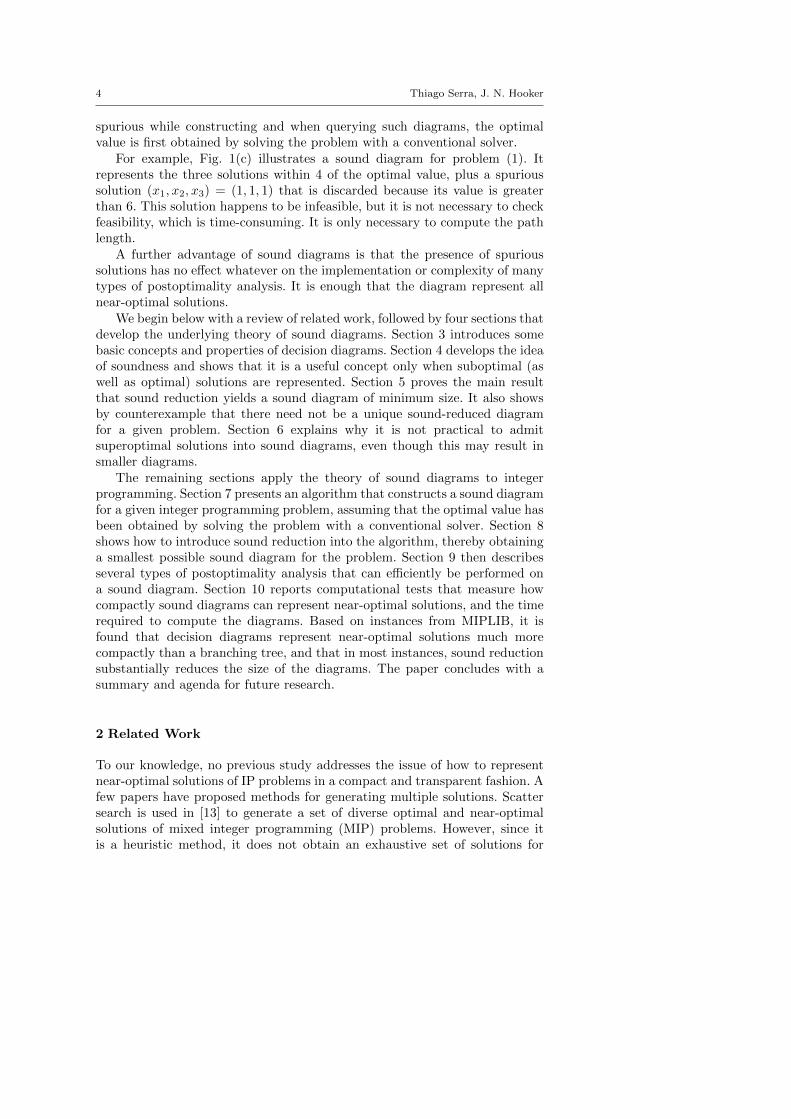
18 Thiago Serra, J. N. Hooker
Algorithm 3 Revisits nodes already explored for updating and re-branching1: procedure RevisitNodes()2: while RevisitBFSQueue 6= ∅ do3: (j, u)← RevisitBFSQueue.pop()4: if u.closed then5: ReopenNode(u) . Procedure below6: end if7: for α ∈ Sj do8: if @a = (u, v) ∈ A : l(a) = α then . Branches again on absent α9: u.openArcs← u.openArcs + 1
10: TryBranching(j, u, α) . Algorithm 211: else12: if w(r, u) + cjα < w(r, v) then . Improves w(r, v)13: w(r, v)← w(r, u) + ciα14: if v.explored then15: RevisitBFSQueue.add(j + 1, v)16: end if17: end if18: end if19: end for20: if u.openArcs = 0 then . Nodes following u remained closed21: CloseNode(j, u) . Algorithm 422: end if23: end while24: end procedure
Subroutine: Reopens nodes in bottom-up order recursively
25: procedure ReopenNode(u)26: u.closed← false27: for all a = (v, u) ∈ A do . Opens all nodes above28: if v.closed then29: ReopenNode(v)30: v.openArcs← 131: else32: v.openArcs← v.openArcs + 133: end if34: end for35: end procedure
w(r, u) + LCDSj [v, u] ≤ z∗+∆. We can therefore sound-reduce u into v when
w(r, u) + min{
LCDSj [u, v],LCDSj [v, u]}> z∗ +∆
The analogous test for sound-reducing v into u occurs in lines 23–26. Theremoval of a node during sound reduction may disconnect subsequent nodesin the diagram, which are removed by the subroutine at the bottom of Algo-rithm 5.
Sound reduction is relatively efficient. Algorithm 5 is called O(nW ) times,whereW is the maximum width of a layer. Each call checksO(W ) nodes havingO(Smax) arcs each, where Smax is the size of the largest variable domain. Thistotals O(nW 2Smax) operations before node removals. Each call of the bottomprocedure requires time O(Smax), for a total time of O(nWSmax).

Compact Representation of Near-Optimal Integer Programming Solutions 19
Algorithm 4 Closes nodes and performs bottom-up processing recursively1: procedure CloseNode(j, u)2: u.closed← true3: for all a = (u, v) ∈ A do . Computes minimum cost path to t4: w(u, t)← min{w(u, t), cj`(a) + w(v, t)}5: end for6: if w(r, u) + w(u, t) > z∗ +∆ then . Node is not minimal7: RemoveDeadendNode(i, u) . Subroutine in Algorithm 18: end if9: for all a = (u, v) ∈ A do
10: if w(r, u) + cj`(a) + w(u, t) > z∗ +∆ then . Arc is not minimal11: A← A \ {a}12: end if13: end for14: ClosingQueue← {}15: for all a = (v, u) ∈ A do16: if ¬v.closed then17: v.openArcs← v.openArcs− 118: if v.openArcs = 0 then . Closes node above19: ClosingQueue← ClosingQueue ∪ {(j, u)}20: end if21: end if22: end for23: CompressDiagram(j, u) . Algorithm ?? or 524: while ClosingQueue 6= ∅ do25: (j, u)← ClosingQueue.pop()26: CloseNode(j, u)27: end while28: end procedure
9 Postoptimality Analysis
Because a sound decision diagram transparently represents all near-optimalsolutions, a wide variety of postoptimality analyses can be conducted withminimal computational effort. We describe a few of these here.
The most basic postoptimality task is to retrieve all feasible solutions whosecost is within a given distance of the optimal cost. That is, we wish to retrieveall δ-optimal solutions from a diagram D that is sound for P(∆), for a desiredδ ∈ [0, ∆]. This is accomplished by Algorithm 6. The algorithm assumes thatthe weight w(r, u) of a minimum-weight path from r to each node u has beenpre-computed in a single top-down pass. Then, for each desired tolerance δ,the algorithm finds δ-optimal solutions in a bottom-up pass. It accumulates foreach node u a set Sufδ(u) of suffixes that could be part of a δ-optimal solution,based on the weight of a minimum-weight r–u path. When the algorithmreaches the root r, Sufδ(r) is precisely the set Sufδ(r) of δ-optimal solutions,because at this point the exact cost of solutions is known.
The worst-case complexity of the algorithm is proportional to the numberof solutions D represents, including spurious solutions. However, many spuri-ous solutions are screened out as the algorithm works its way up, particularly

20 Thiago Serra, J. N. Hooker
Algorithm 5 Sound-reduces node u with another closed node if possible1: procedure CompressDiagram(j, u)2: for all v ∈ Uj : v 6= u ∧ v.closed, and v ordered by nondecreasing w(r, d) do3: LCDSj [u, v],LCDSj [v, u]←∞4: for all α ∈ Sj do5: if ∃au = (u, u+) : `(au) = α then6: if ∃av = (v, v+) : `(av) = α then7: LCDSj [u, v]← min{LCDSj [u, v], w(au) + LCDSj+1[u+, v+]}8: LCDSj [v, u]← min{LCDSj [v, u], w(au) + LCDSj+1[v+, u+]}9: else
10: LCDSj [u, v]← min{LCDSj [u, v], w(au) + w(u+, t)}11: end if12: else13: if ∃av = (v, v+) : `(av) = α then14: LCDSj [v, u]← min{LCDSj [v, u], w(av) + w(v+, t)}15: end if16: end if17: end for18: if w(r, v) ≤ w(r, u) then19: if w(r, u) + min{LCDSj [u, v],LCDSj [v, u]} > z∗ +∆ then20: SoundReduce(j, u, v) . First procedure below21: break22: end if23: else if w(r, v) + min{LCDSj [u, v],LCDSj [v, u]} > z∗ +∆ then24: SoundReduce(j, v, u) . First procedure below25: break26: end if27: end for28: end procedure
Subroutine: Sound-reduces node u into node v at level j
29: procedure SoundReduce(j, u, v)30: for all a = (q, u) ∈ A do31: a← (q, v) . Redirects arcs to v32: end for33: v.lhs← ∅ . Removes v’s state34: RemoveIfDisconnected(j, u) . Next procedure below35: end procedure
Subroutine: Removes node u ∈ Uj and subsequent disconnected nodes in D
36: procedure RemoveIfDisconnected(j, u)37: if @a = (v, u) ∈ A then38: Uj ← Uj \ {u}39: for all a = (u, v) ∈ A do40: A← A \ {a}41: RemoveIfDisconnected(j + 1, v)42: end for43: end if44: end procedure
because a solution with cost greater than z∗ + δ (where possibly δ � ∆) canbe discarded. Retrieval can therefore be quite fast for small δ.
The same algorithm can answer a number of postoptimality questions. Forexample, one might ask which solutions are δ-optimal when certain variablesare fixed to certain values—or, more generally, when the domains Sj of certain

Compact Representation of Near-Optimal Integer Programming Solutions 21
Algorithm 6 Retrieves δ-optimal solutions from a sound diagram for δ ∈[0, ∆]
1: function RetrieveSolutions(δ)2: Sufδ(t) = {null} . Sufδ(u) = set of possible δ-suffixes of u3: w(null) = 0 . null is the zero-length suffix.4: for j = n→ 1 do . Retrieve δ-optimal solutions in bottom-up pass.5: for all u ∈ Uj do
6: Sufδ(u) = ∅7: for all a = (u, v) ∈ Aj do
8: for all s ∈ Sufδ(v) do . Examine suffixes of v.9: if w(r, u) + w(a) + w(s) ≤ z∗ + δ then . Possible new δ-suffix of u?
10: Sufδ(u)← Sufδ(u) ∪ {`(a)||s} . Append `(a) to suffix s.11: w(`(a)||s) = w(`(a)) + w(s) . Compute weight of new suffix.12: end if13: end for14: end for15: end for16: end for17: return Sufδ(r) . Returns set of δ-optimal solutions.18: end function
variables are replaced by proper subsets S′j of those domains. This is easilyaddressed by removing, for each S′j , all arcs leaving layer j with labels thatdo not belong to S′j . Algorithm 6 is then applied to the smaller diagram thatresults, after recomputing weights w(r, u). Since the use of smaller domainsdoes not add any ∆-optimal solutions, no δ-optimal solutions are missed.Methods for efficient updating of shortest paths are discussed in [25].
One might also ask which solutions are δ-optimal when the objective func-tion coefficients are altered, say to c′. Since changing the cost coefficients canintroduce ∆-optimal solutions, the sound diagram may fail to represent somesolutions that are ∆-optimal for the altered costs. However, we can identify allsolutions that remain δ-optimal after the cost change for δ ≤ ∆−∑n
j=1 |c′j−cj |since all of those were originally ∆-optimal. This is accomplished simply bymodifying the arc weights to reflect the new costs and running Algorithm 6,again with recomputed weights w(r, u).
Several additional types of postoptimality analysis can be performed, allwith the advantage that spurious solutions have no effect on the computations.These types of analysis can therefore be conducted very rapidly.
For example, we can determine the values that a given variable can takesuch that the resulting minimum cost is within δ of the optimum. We referto this as the δ-optimal domain of the variable. For each variable xj , weneed only scan the arcs leaving layer j and observe which ones pass test (2)when ∆ is replaced with δ. This is done in Algorithm 7, which computesδ-optimal domains for all variables. In particular, the solution value of xj isinvariant across all δ-optimal solutions if its δ-optimal domain is a singleton.The algorithm assumes that shortest path lengths w(r, u) and w(u, t) have beenpre-computed for each node u. Its complexity is dominated by the complexityO(nW 2) of computing the shortest path lengths. The algorithm can also be

22 Thiago Serra, J. N. Hooker
Algorithm 7 Computes δ-optimal domains for all variables, where δ ∈ [0, ∆]
1: procedure ComputeNearOptimalDomains(δ)2: for j = 1→ n do3: Xj ← ∅ . Xj is the subset of Sj in δ-optimal solutions.4: for all a = (u, v) ∈ Aj : `(a) /∈ Xj do . Loops on arcs of missing values5: if w(r, u) + w(a) + w(v, t) ≤ x∗ + δ then6: Xj ← Xj ∪ {`(a)} . Found a δ-optimal solution where xj = `(a)7: end if8: end for9: end for
10: end procedure
Algorithm 8 Computes the cost coefficient c′j for each variable xj on 0–1 domains that yields optimal solutions with xj = 0 and xj = 1 among thesolutions of the decision diagram, if the other cost coefficients remain the same1: function ComputeIndifferentCostCoefficients()2: for j = 1→ n do3: for α ∈ {0, 1} do4: zα ←∞ . zα is min
∑j′ 6=j cj′xj′ when xj = α
5: end for6: for all a = (u, v) ∈ Aj do7: if w(r, u) + w(v, t) < z`(a) then8: z`(a) ← w(r, u) + w(v, t) . Found a lower value of
∑j′ 6=j cj′xj′
9: end if10: end for11: if z0 =∞ then . There is no solution with xj = 012: c′j =∞13: else if z1 =∞ then . There is no solution with xj = 114: c′j = −∞15: else . There are solutions for both assignments16: c′j = z0 − z1 . Coefficient for which z0 = z1 + c′j17: end if18: end for19: return c′
20: end function
run after the domains of certain variables are replaced with proper subsets ofthose domains, to determine the effect on the δ-optimal domains of the othervariables.
We can also perform range analysis for individual cost coefficients cj . Aswith the previous analysis, the presence of spurious solutions has no effect.For each variable xj , we can look for the values of cj that would make eachvalue in the domain of xj optimal, provided that the other cost coefficients areunchanged. This idea is particularly simple and insightful when the domainsare binary, as described in Algorithm 8: if there are solutions in the diagramfor which xj = 0 and xj = 1, there is a unique value c′j for which thereare alternate optima with both values. Any cj > c′j makes solutions wherexj = 1 suboptimal, and conversely any cj < c′j makes solutions where xj = 0suboptimal. If applied to solutions that were originally ∆-optimal, the outcomeremains valid as long as cj does not change more than ∆.

Compact Representation of Near-Optimal Integer Programming Solutions 23
10 Computational Experiments
The experiments were designed to assess the compactness of sound decisiondiagrams, based on 0–1 problem instances in MIPLIB. We constructed threedata structures for each of 12 instances and a range of tolerances ∆. The firststructure is a branching tree T that represents all ∆-optimal solutions. Thesecond is the sound diagram U that is obtained from Algorithms 1–4, butomitting the sound-reduction step in Algorithm 5. The third is the sound-reduced diagram S that is obtained by applying Algorithms 1–5. DiagramS is therefore a smallest possible sound diagram for the problem instance.By comparing the size U with the size of T , we can see the advantage ofrepresenting solutions with a sound decision diagram in which equivalent statesare unified. By comparing the size of S with the size of U , we can measure theadditional advantage obtained by sound reduction.
We carried out the experiments for tolerances ∆ that range over a wideinterval from zero to ∆max in increments of 0.1∆max. For the smaller instances,we set ∆max large enough to encompass all feasible solutions; that is, largeenough so that all feasible solutions are ∆max-optimal. These instances arebm23, enigma, p0033, p0040, stein9, stein15, and stein27. Thus for theseinstances, ∆max is the difference in value between the best and worst solutions.For the remaining instances, we set ∆max equal to the median absolute valueof nonzero objective coefficients. This allows us to test variations of up to100% in objective coefficients of half of these variables. If the runtime was lessthat 1000 seconds, we kept doubling ∆max until the runtime exceeded 1000seconds, but stopped short of a doubling that resulted in a runtime of morethan 24 hours.
In all experiments, the branching priority is DFS, variables are ordered byincreasing index, and 0-arcs are explored before 1-arcs. The code is written inC++ (gcc version 4.8.24), uses the COIN-OR CLP solver1 (version 1.16.10),and ran in Ubuntu 14.04.2 LTS on a machine with Intel(R) Xeon(R) CPUE5-2680 v3 @ 2.50GHz processors and 128 GB of RAM.
Table 2 displays the statistics for the maximum tolerance ∆max, includingthe number of optimal and ∆max-optimal solutions, and the size and con-struction time for T , U , and S. The sound-reduced diagram S is dramaticallysmaller than the branching tree T for all the instances except enigma. It is alsosignificantly smaller than the unified diagram U except in the cases of air01and enigma, and smaller by at least an order of magnitude in three instances.On the other hand, sound reduction added significantly more computationtime to the diagram construction in seven of the instances.
In practice, the desired tolerance ∆ is typically much less than ∆max. Wetherefore display in Figs. 6–7 how the diagram sizes and computation timesdepend on ∆ for six of the instances. Note that the diagram sizes and runtimesare plotted on a logarithmic scale. As predicted by Corollary 1, the diagramsize is monotone nondecreasing in ∆.
1 projects.coin-or.org/Clp
24 Thiago Serra, J. N. Hooker
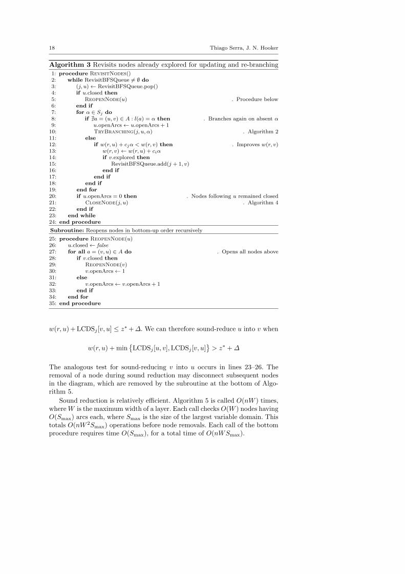
Table 2: Solution counts, with diagram sizes and construction times, for MIPLIB instancesusing a maximum tolerance ∆max.
Instance ∆maxSolutions Size (nodes) Runtime (s)
Opt. ∆max-opt. T U S U S
air01 3194 2 16,899 5,058,113 61,652 61,652 340 11,000bm23∗ 59 1 2,168 23,620 20,356 5,460 31 40enigma∗ 1 2 4 278 243 243 41 41lseu 236.16 2 67,250 2,057,264 294,108 53,465 2,900 8,600mod008 21 6 4,954 891,543 188,359 38,292 15,000 16,000p0033∗ 2112 9 10,746 55,251 847 449 5.8 33p0040∗ 7102 1 519,216 2,736,899 2,950 831 2.6 620p0201 375 4 34,504 2,326,052 107,312 6,627 1,900 7,700sentoy 280.8 1 85,401 1,868,562 1,754,681 101,618 3,800 12,000stein9∗ 4 54 172 460 137 80 0.02 0.05stein15∗ 6 315 2,809 8,721 2,158 816 0.54 1.6stein27∗ 9 2,106 367,525 1,450,702 338,916 25,444 159 1,400
∗∆max set large enough to include all feasible solutions.
The sound-reduced diagram S is substantially more compact than thebranching tree T in every instance. It is also smaller than U in all instancesbut one, although one must normally pay a higher computational price forthis reduction. Of course, a sound-reduced diagram need only be generatedonce in order to carry out a large number of postoptimality queries. Thesound-reduced diagrams for typical values of ∆ are well within a practicalsize range for rapid postoptimality processing, normally a few hundred or afew thousand nodes. The computation times for constructing diagrams of thissize are likewise modest, ranging from a few seconds to a few minutes.
11 Conclusion
We explored sound decision diagrams as a data structure for concisely andtransparently representing near-optimal solutions of integer programming prob-lems. We showed that repeated application of a simple sound-reduction stepyields a smallest possible sound diagram for any given discrete optimizationproblem. Based on this result, we stated an algorithm for constructing sound-reduced diagrams for integer programming problems. We showed how theresulting diagrams permit several types of postoptimality analysis, and thatthe presence of spurious solutions in the diagrams has no effect on mosttypes of analysis. Computational testing indicates that sound-reduced dia-grams generally offer dramatic reductions in the space required to representnear-optimal solutions, relative to that required by a branching tree. For theMIPLIB instances tested, the resulting diagrams are well within a size rangethat permits rapid postoptimality processing.
This study is inspired by the idea that solution of an optimization problemshould be viewed more broadly than merely generating one or more optimalsolutions. Rather, it should be seen as transforming an opaque data structurethat defines the problem but does not reveal its solutions, to a transparent datastructure that provides ready access to optimal and suboptimal solutions of

Compact Representation of Near-Optimal Integer Programming Solutions 25
0 10 20 30 40 50
102
103
104
Near-optimal gap ∆
Nodes
(a1) Representation sizes for bm23
TUS
0 10 20 30 40 50
100
101
Near-optimal gap ∆
Runtime(s)
(b1) Construction time for bm23
US
0 1,000 2,000 3,000 4,000 5,000 6,000 7,000
102
103
104
105
106
Near-optimal gap ∆
Nodes
(a2) Representation sizes for p0040
TUS
0 1,000 2,000 3,000 4,000 5,000 6,000 7,000
10−1
100
101
102
103
Near-optimal gap ∆
Runtime(s)
(b2) Construction time for p0040
US
0 2 4 6 8
104
105
106
Near-optimal gap ∆
Nodes
(a3) Representation sizes for stein27
TUS
0 2 4 6 8101
102
103
Near-optimal gap ∆
Runtime(s)
(b3) Construction time for stein27
US
Fig. 6: Diagram size and computation time vs. ∆ for three smaller instances.
interest. We attempted to lay a foundation for this type of solution for integerprogramming, but an obvious research direction is to extend the method tomixed integer programming. Decision diagrams can continue to play a role,

26 Thiago Serra, J. N. Hooker
0 500 1,000 1,500 2,000 2,500 3,000
103
104
105
106
107
Near-optimal gap ∆
Nodes
(a1) Representation sizes for air01
TUS
0 500 1,000 1,500 2,000 2,500 3,000
101
102
103
104
Near-optimal gap ∆
Runtime(s)
(b1) Construction time for air01
US
0 50 100 150 200
102
103
104
105
106
Near-optimal gap ∆
Nodes
(a2) Representation sizes for lseu
TUS
0 50 100 150 200
102
103
104
Near-optimal gap ∆
Runtime(s)
(b2) Construction time for lseu
US
0 5 10 15 20
103
104
105
106
Near-optimal gap ∆
Nodes
(a3) Representation sizes for mod008
TUS
0 5 10 15 20
102
103
104
Near-optimal gap ∆
Runtime(s)
(b3) Construction time for mod008
US
Fig. 7: Diagram size and computation time vs. ∆ for three larger instances.
because paths in a diagram can represent values for the integer variables inthe problem.

Compact Representation of Near-Optimal Integer Programming Solutions 27
References
1. Achterberg, T., Heinz, S., Koch, T.: Counting solutions of integer programs usingunrestricted subtree detection. In: L. Perron, M.A. Trick (eds.) Proceedings of CPAIOR,pp. 278–282. Springer (2008)
2. Akers, S.B.: Binary decision diagrams. IEEE Transactions on Computers C-27, 509–516(1978)
3. Andersen, H.R., Hadzic, T., Hooker, J.N., Tiedemann, P.: A constraint store basedon multivalued decision diagrams. In: C. Bessiere (ed.) Principles and Practice ofConstraint Programming (CP 2007), Lecture Notes in Computer Science, vol. 4741,pp. 118–132. Springer (2007)
4. Arthur, J.A., Hachey, M., Sahr, K., Huso, M., Kiester, A.R.: Finding all optimalsolutions to the reserce site selection problem: Formulation and computational analysis.Environmental and Ecological Statistics 4, 153–165 (1997)
5. Bergman, D., Cire, A.A., van Hoeve, W.J., Hooker, J.N.: Discrete optimization withbinary decision diagrams. INFORMS Journal on Computing 28, 47–66 (2016)
6. Bryant, R.E.: Graph-based algorithms for Boolean function manipulation. IEEETransactions on Computers C-35, 677–691 (1986)
7. Camm, J.D.: ASP, the art and science of practice: A (very) short course in subopti-mization. Interfaces 44(4), 428–431 (2014)
8. Danna, E., Fenelon, M., Gu, Z., Wunderling, R.: Generating multiple solutions for mixedinteger programming problems. In: M. Fischetti, D.P. Williamson (eds.) Proceedings ofIPCO, pp. 280–294. Springer (2007)
9. Dawande, M., Hooker, J.N.: Inference-based sensitivity analysis for mixed integer/linearprogramming. Operations Research 48, 623–634 (2000)
10. Gamrath, G., Hiller, B., Witzig, J.: Reoptimization techniques for MIP solvers. In:E. Bampis (ed.) Proceedings of SEA, pp. 181–192. Springer (2015)
11. GAMS Support Wiki: Getting a list of best integer solutions of my MIP (2013). URLhttps://support.gams.com
12. Geoffrion, A.M., Nauss, R.: Parametric and postoptimality analysis in integer linearprogramming. Management Science 23(5), 453–466 (1977)
13. Glover, F., Løkketangen, A., Woodruff, D.L.: An annotated bibliography for post-solution analysis in mixed integer programming and combinatorial optimization. In:M. Laguna, J.L. Gonzalez-Velarde (eds.) OR Computing Tools for Modeling, Opti-mization and Simulation: Interfaces in Computer Science and Operations Research, pp.299–317. Kluwer (2000)
14. Goetzendorff, A., Bichler, M., Shabalin, P., Day, R.W.: Compact bid languages and corepricing in large multi-item auctions. Management Science 61(7), 1684–1703 (2015)
15. Greistorfer, P., Løkketangen, A., Voß, S., Woodruff, D.L.: Experiments concerningsequential versus simultaneous maximization of objective function and distance. Journalof Heuristics 14, 613–625 (2008)
16. Hadzic, T., Hooker, J.N.: Discrete global optimization with binary decision diagrams.In: Workshop on Global Optimization: Integrating Convexity, Optimization, LogicProgramming, and Computational Algebraic Geometry (GICOLAG). Vienna (2006)
17. Hadzic, T., Hooker, J.N.: Postoptimality analysis for integer programming using binarydecision diagrams. Tech. rep., Carnegie Mellon University (2006)
18. Hadzic, T., Hooker, J.N.: Cost-bounded binary decision diagrams for 0–1 programming.In: P. van Hentemryck, L. Wolsey (eds.) CPAIOR Proceedings, Lecture Notes inComputer Science, vol. 4510, pp. 332–345. Springer (2007)
19. Hoda, S., van Hoeve, W.J., Hooker, J.N.: A systematic approach to MDD-based con-straint programming. In: Proceedings of the 16th International Conference on Principlesand Practices of Constraint Programming, Lecture Notes in Computer Science. Springer(2010)
20. Holm, S., Klein, D.: Three methods for postoptimal analysis in integer linear program-ming. Mathematical Programming Study 21, 97–109 (1984)
21. Hu, A.J.: Techniques for efficient formal verification using binary decision diagrams.Thesis CS-TR-95-1561, Stanford University, Department of Computer Science (1996)
28 Thiago Serra, J. N. Hooker
22. IBM Support: Using CPLEX to examine alternate optimal solutions (2010). URLhttp://www-01.ibm.com/support/docview.wss?uid=swg21399929
23. Kilinc-Karzan, F., Toriello, A., Ahmed, S., Nemhauser, G., Savelsbergh, M.: Approx-imating the stability region for binary mixed-integer programs. Operations ResearchLetters 37, 250–254 (2009)
24. Lee, C.Y.: Representation of switching circuits by binary-decision programs. BellSystems Technical Journal 38, 985–999 (1959)
25. Miller-Hooks, E., Yang, B.: Updating paths in time-varying networks given arc weightchanges. Transportation Science 39, 451–464 (2005)
26. Schrage, L., Wolsey, L.: Sensitivity analysis for branch and bound integer programming.Operations Research 33, 1008–1023 (1985)
27. Van Hoesel, S., Wagelmans, A.: On the complexity of postoptimality analysis of 0/1programs. Discrete Applied Mathematics 91, 251–263 (1999)
28. Wegener, I.: Branching Programs and Binary Decision Diagrams: Theory and Applica-tions. Society for Industrial and Applied Mathematics (2000)