1

Instructor: Alexander Barg (abarg@umd.edu) Office: AVW2361

Course goals: To introduce the main concepts of coding theory and the body of its central results.

Prerequisites for the courseThe main prerequisite is mathematical maturity, in particular, interest in learning new mathematical concepts. No familiarity with information theory and communications-related courses will be assumed. On the other hand, the students are expected to be comfortable with linear spaces, elementary probability and calculus, and elementary concepts in discrete mathematics such as binomial coefficients and an assortment of related facts. There is no required textbook.

The web site http://www.ece.umd.edu/~abarg/626 containsa detailed list of topics, problems, schedule of exams, grading policy, reference books.

ENEE626, CMSC858B, AMSC698B

Error Correcting Codes

2

Part I. Introduction to coding theory

3

Plan for today:1. Syllabus, logistics2. Model of a communication system3. Binary Symmetric Channel4. Coding for error correction5. Notation and language

Digital communication: Computer networks, wireless telephony, dataand media storage, RF communication (terrestrial, space)

Transmission over communication channels is prone to errors.background noise, mutual interference between users, attenuation in channels,mechanical damage, multipath propagation, …

4

source coder channel decoder destination

Model of a communication system

more detailed:

sourcesource coder

(compression)

modulator channel

demodulator

channelcoder

channel decoder(error correction)

sourcedecoderdestination

5

source coder channel decoder destination

Model of a communication system

more detailed:

sourcesource coder

(compression)

modulator channel

demodulator

channelcoder

channel decoder(error correction)

sourcedecoderdestination

we are interested in

6

Assume transmission with binary antipodal signals over a Gaussianchannel

Suppose that the received signal y is decoded asx=sgn(y) s

The probability of error is computed as

+s-s

N(s,σ2)

7

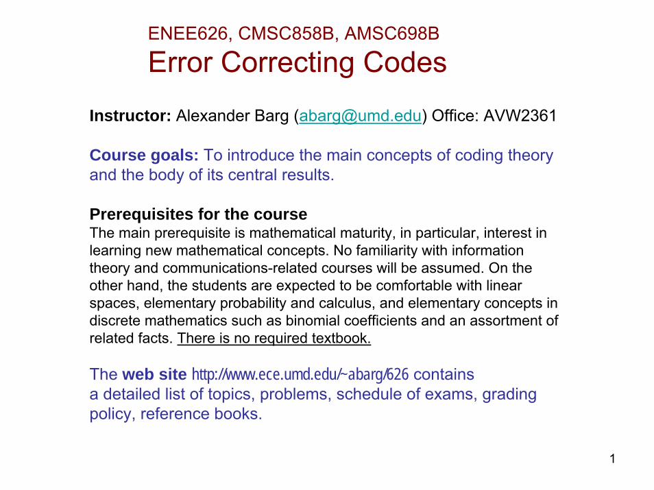
Binary Symmetric Channel (BSC)

0

1

0

1

1-p

1-p

p

p

transmissions are independent

p is called the transition (cross-over) probability

Much of coding theory deals with error correction for transmissionover the BSC. This will also be our main underlying model.

8

Binary Symmetric Channel (BSC)

0

1

0

1

1-p

1-p

p

p

transmissions are independent

p is called the transition (cross-over) probability

Much of coding theory deals with error correction for transmissionover the BSC. This will also be our main underlying model.

The erasure channel

0 0

1 1

? (erasure)

1-p

p

p

1-p

Main example:internet traffic

9

Messages = binary strings Ex.: 101

k bits (m1,m2,...,mk) word, vector mi∈{0,1}

encoding: message codeword. purpose: error correction

Example: 2 messages 0,1.

no coding: 0 → channel → 1 (message lost)

encode 0 → 000 C={000,111} – a code1 → 111

000 → channel → 010

Pr[0|010]=p(1-p)2Pr[0]/Pr[010]; Pr[1|010]=p2(1-p) Pr[1]/Pr[010]

Pr[0|010] Pr[1|010]

Thus, if p<1/2, Pr[0|010]>Pr[1|010].Conclude: decoding by maximum a posteriori probability (MAP) will recover the message correctly

=(1-p)/p > 1 if p<1/2.

10

Definition 1.2: Hamming distance between two vectors x,yd((x1,x2,...,xn),(y1,y2,...,yn))=|{i:xi ≠ yi}|

Transmit M=2k messages with a code C= {x1,x2,…xM}

y received from the channel. Decode to

x = argmin d(xi,y) (minimum distance decoding)xi∈ C

(if there are several such x, declare an error)

Observation: on the BSC(p), p<½, the probability Pr[e] of error e=(e1,e2,e3) decreases as the # of 1’s among e1,e2,e3 increases. Hence, decoding by minimum distance is equivalent to MAP decoding

Conclude: it’s a good idea in many cases to have codewords far apart

11

Bits of notation

Finite sets A,B,C,F, ...The number of elements in A is called the size of A, denoted |A| or #(A).

F2={0,1} the binary field; F=F2n – n-dim linear space over F2

x,y,... – vectors (often in F) (row vectors); xT transpose (column vect.)0=0n the all-zero vector; likewise, (0i1j...) is a generic shorthand for a vector(x,y)=∑i=0

n xi yi dot productd(x,y) = |{i: xi≠ yi}| Hamming distance w(x) (sometimes wt(x)) the weight of x, i.e., d(x,0)

G,H,A,... matrices

d(C) = the distance of the code CC[n,k,d] a linear code of length n, dimension k, distance dC(n,M,d) a code, not necessarily linear, of length n, size M, distance d

12

Mathematical concepts used in coding theory

The primary language is that of linear algebra.Linear algebra deals with geometry of linear spaces and their transformations

A linear space L is the most familiar concept, such as R2, R3 and the likesIt is formed of a field of constants (e.g., R) and vectors over itVectors obey the natural rules:they can be added to form another vector; they can be stretched by multiplyingthem by a constant.

To describe L it is convenient to choose a basis (a frame). The numberof vectors in the basis is called the dimension of L.The space does not depend on the choice of the basis although thecoordinates of the vectors generally change if one passes to another basis

A subspace M of L can be described by any of its bases or asa set of solutions of a system of equations (kernel of a linear operator)

The quotient space L/M consists of M and its shifts by vectors from L\MLinear spaces of coding theory live over finite fields (such as F2={0,1}).

13

Reminder (cont'd): binomial coefficients

x∈R

(a) Permutations: (abc, acb, bac, bca, cba, cab)n(n-1)(n-2)…2 .1=n! (n factorial)

(b) The number of ways to choose an ordered k-tuple out of an n-setn(n-1)(n-2)…(n-k+2)(n-k+1)=(n)k

(c) The number of unordered k-tuples out of an n-set.

notation: 1 0 1 1 1

1 2 1 21 3 3 1 3

1 4 6 4 1 41 5 10 10 5 1 5

1 6 15 20 15 6 1 61 7 21 35 35 21 7 1 7|{x ∈ F: wt(x)=k}|=

Extend the definition:

See probl. 12, h/work 1

14

Operating with binary data

XOR AND

+ 0 1 • 0 10 0 1 0 0 01 1 0 1 0 1

x1=(01101), x2=(10101)x1 + x2=(11000)(x1,x2)=∑i=1

n x1,ix2,i (dot product)

(x1,x2)=0 or 1 according as #i such that x1,i=x2,i=1 is even or odd

Notation: F2={0,1}; F=(F2)n

15

code can correct one error, can be used totransmit 8=23 messages (3 bits of information)

Examples of codes:

m1 000 a 000000m2 001 a 001111m3 010 a 010110m4 011 a 011001m5 100 a 100101m6 101 a 101010m7 110 a 110011m8 111 a 111100

Repetition code {000…00,111…11} k=1Single parity-check code {x1,x2,…,xM} formed of all codewords of length

n with an even number of ones. M=2n-1

n=3: {000,011,101,110}

Goal: construct codes of arbitrary length that correct a given numberof errors, equipped with a simple decoding procedure

16

ENEE626 Lecture 2: Linear codes

1. Linear codes: examples, definition2. Generator and parity-check matrices3. Hamming weight4. Algorithmic complexity

17

Therefore, is closed under addition:

xi + xj = (mi + mj) G= mk G=xk ∈

Verify that all the codewords of can be computed by multiplying

xi = mi G, where

100101G= 010110

001111

m6G=(101)G=101010=x6

is a linear code (a linear subspace of (F2)n )

Linear codesCode C

m1 000 a 000000m2 001 a 001111m3 010 a 010110m4 011 a 011001m5 100 a 100101m6 101 a 101010m7 110 a 110011m8 111 a 111100

18

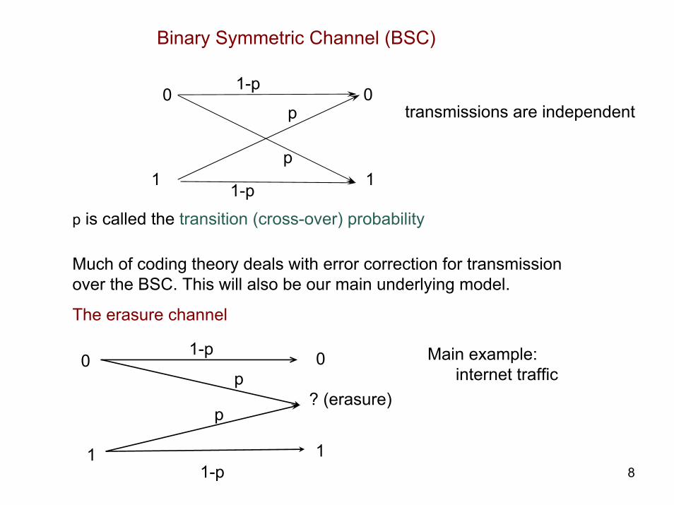
F=(F2)n is a linear space:

• F is an abelian group under addition• Its unit is the all-zero vector 0=(00...000)• Multiplication by scalars is distributive

c(x+y)=cx+cy(a+b)x=ax+bx

• Multiplication is associative:(ab)x = a(bx)

Definition 2.1: A linear subspace of F is called a binary linear code

For instance, the code above is linear

Let A be a linear code, k=dim A. A matrix whose rows are the basisvectors of A is called a generator matrix of the code.

G (kxn)-matrix

19

Example: let n=4, consider 4-dim space F0000000100100011 x1 x20100 2-dim subspace h0001, 0010i (h , i means linear hull)0101 0110 C = { λ1x1+λ2x2, λ1,λ2∈{0,1} } 0111 00011000 Explicitly, C={0000,0001,0010,0011} G= 001010011010 Generally, |C|=2k, where k is the dimension of the code1011 1100110111101111

20

n is called the length of the code.

Consider the code A={00000,11111} of length 5, dimension 1

G=[11111]

(the repetition code).

Single parity-check code B, n=5 G=

Definition 2.2: The Hamming weight of a vector x=(x1,...,xn) is defined asw(x)=|{i : xi=1}|

Exercise: The sum of two even-weight vectors has even weight.

Thus, the code B is formed of 24=16 vectors of even weight(satisfies an overall parity check)

21

The parity-check matrix of a code

Consider a code of length 6: x=(x1,x2,x3,x4,x5,x6)Suppose that

x1 + x2 + x3 + x4 =0x2 + x3 + x5 =0

x1 + x3 + x6=0

Assign any values to x1,x2,x3, solve for x4,x5,x6

Parity-check equations

H xT=0

Definition 2.3: H is called a parity-check matrix of the code

Another definition of a linear code: C={x ∈ F: H xT=0}

22

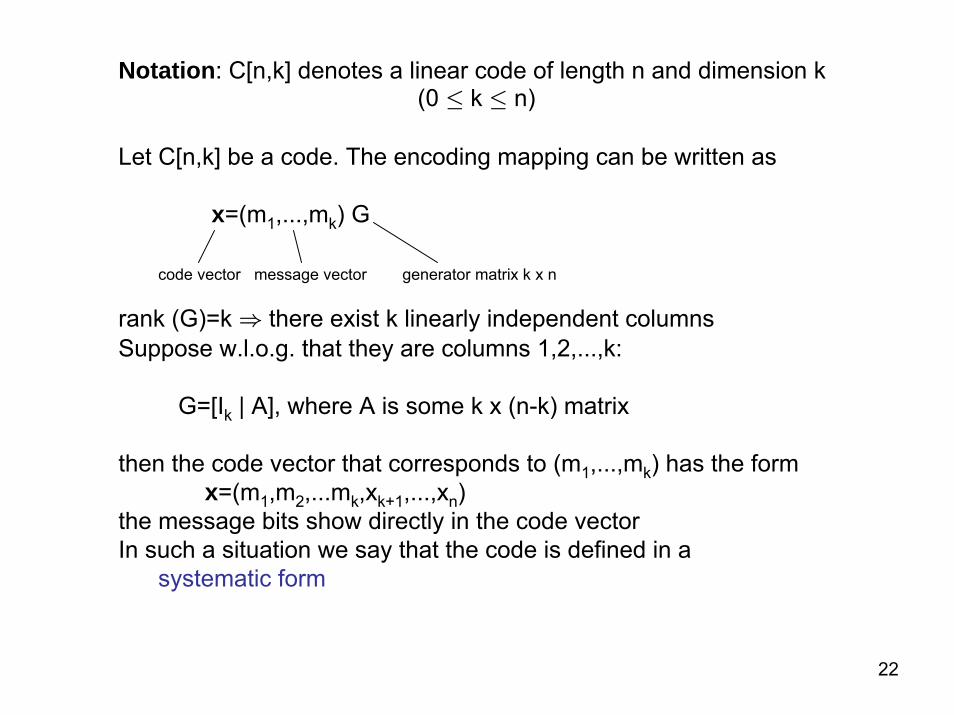
Notation: C[n,k] denotes a linear code of length n and dimension k(0 · k · n)

Let C[n,k] be a code. The encoding mapping can be written as

x=(m1,...,mk) G

code vector message vector generator matrix k x n

rank (G)=k ⇒ there exist k linearly independent columnsSuppose w.l.o.g. that they are columns 1,2,...,k:

G=[Ik | A], where A is some k x (n-k) matrix

then the code vector that corresponds to (m1,...,mk) has the formx=(m1,m2,...mk,xk+1,...,xn)

the message bits show directly in the code vectorIn such a situation we say that the code is defined in a

systematic form

23

Proposition 2.1: Any [n,k] linear code can be written in a systematic form

Indeed, take the k columns of G that have rank k; by elementaryoperations diagonalize this submatrix

Example: The matrix

defines the single-parity-check code of length 5 in a systematic form: the last 4 coordinates carry the message, the first coordinate corresponds to the parity check. For instance, the message (1101) is encoded as (11101)

G=

Note that we can have message symbols in any 4 of the 5 coordinates:

for instance, the matrix defines the same code as in Example 2.2,

which has been written in a systematic form to show the message bits in coordinates1,3,4,5.

Lemma 2.2: Let G=[Ik|A] be a k x n generator matrix of a code C. Then H=[AT|In-k]is a parity-check matrix of C.

Proof:

24

Encoding in a systematic form

G=[Ik | A], A a k x (n-k) matrix with rows a1,...ak

mG=(m1,...,mk, a), where a=∑i mi ai

Let H=[AT|In-k] be the p.-c. matrix. The parity check symbols are computedfrom the equations HxT=0, where x=(m1,...,mk,x1,x2,...,xn-k). Thus,

m1 a1,1 +m2 a2,1 +...+mk ak,1+x1 =0m1 a1,2 +m2 a2,2 +...+mk ak,2 + x2 =0....m1 a1,n-k+m2 a2,n-k+...+mk ak,n-k + xn-k=0

Encoding in a systematic form is easier than in a general form

25

Definition 2.4: Let x1,x2 ∈ F. The Hamming distance

d(x1,x2) = #{i: x1,i≠ x2,i}

Exercises: 1. Prove that d(·,·) is a metric on F.2. Prove that d is translation invariant, i.e.,

d(x1,x2)=d(x1+y,x2+y)where y∈ F is an arbitrary vector.

Take y=x2, then d(x1,x2)=d(x1+x2,0)Call d(x,0) the weight of x, denoted wt(x)wt(x)=#{i: xi≠ 0}

Definition 2.5: Let C be a linear code. The distance of C is defined as

d(C)=minx1,x2 ∈ C, x1≠x2d(x1,x2)

Exercise: d(C)=minx∈ CÂ 0 wt(x)

26

Example: Consider again the code C={0000,0001,0010,0011}d(C)=1

Notation: We write C[n,k,d] to denote a linear code of length n, dimensionk and distance d.

Linear codes are the main subject of coding theory. We can think ofa linear code as of a mapping C: {0,1}k → {0,1}n.

Remark: Unrestricted codes. A code is an arbitrary subset C ⊂ F.The minimum distance of the code is defined as

d(C)=minx ≠ y; x,y ∈ C d(x,y)

We write C(n,M,d) to denote a code of length n, size M and distance d.Unrestricted codes are described by listing all the codewords or describinga way to generate the codewords. There are many interesting theoreticalproblems related to nonlinear codes. In practical applications, codes arealmost always linear because of complexity constraints.

27

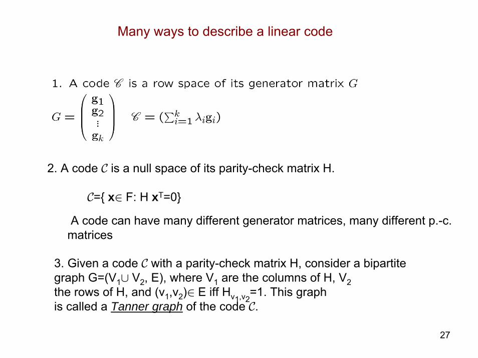
Many ways to describe a linear code

2. A code C is a null space of its parity-check matrix H.

C={ x∈ F: H xT=0}

A code can have many different generator matrices, many different p.-c.matrices

3. Given a code C with a parity-check matrix H, consider a bipartitegraph G=(V1∪ V2, E), where V1 are the columns of H, V2the rows of H, and (v1,v2)∈ E iff Hv1,v2

=1. This graphis called a Tanner graph of the code C.

28

Example: Consider a [7,4,3] code

variablenodes(columns) check

nodes(rows)

Tanner graph representation

An assignment of values to the variable nodes forms a valid codeword if the sum at every check node=0

m1 m2m4

m3

the same graph

29

Complexity of algorithms

An important objective of coding theory is simple processing of data

We shall assume a naive model under which one operation with twobinary digits involves a unit cost.

For instance, computing z=x+y, where x,y,z ∈ (F2)n has complexity n. Likewise, computing (x,y) takes complexity n+(n-1)(n multiplications, n-1 additions).

Computing the Hamming distance d(x,y) takes n operations.

Suppose we are given a code C(n,M) and a vector y∈ (F2)n, want to find x=arg minz∈ C d(y,z). In principle, this can take nM operations.With n growing this becomes prohibitively complex.

We will assume that an algorithm of complexity p(n), where pis some polynomial, is acceptable, an algorithm of exponentialcomplexity is “too difficult” (comparable to exhaustive search).

30

Examples: Let C be a code of size |C|=M.

1. The complexity of encoding for a linear code.Let G be a k x n matrix over F2, let m be a k-vector. The complexityof computing x=m G is O(k n)=O(log2 M)

2. The complexity of ML decoding is O(nM), No shortcuts are known in general for linear codes.

Notation: Let n→∞

f(n)=O(g(n)) ⇔ ∃ const such that f(n)· (const)g(n) Big-O

Coding theory studies families of codes as much as (or more than) individual codes. The primary reason is Shannon’s theorem which saysthat reliable transmission can be achieved at the expense of a growingcode length n. Exact formulation and proof given later.

31

ENEE626 Lecture 3: Linear codes and their decoding

Plan1. Linear codes over alphabets other than binary2. Correctable errors3. Standard array

32

Nonbinary codes

Nonbinary alphabets. Examples: q=3; q=4.

Ternary alphabet Q={0,1,2} with operations mod 3. -1=2 mod 3The set Qn forms a linear space {x1,x2,…,x3n}

000,001,002,010,011,012,020,021,022,100,200,101,….

A ternary linear code C is a linear subspace of Qn. The concepts defined earlier (generator matrix, parity-check matrix, standard array, etc.) are extended straightforwardly.

C[4,2] G= 0 1 2 1 H=1 1 1 01 1 1 1 0 2 0 1

Distance d(C)=min. # of nonzero coordinates in a nonzero code vector. Above: C[4,2,2]

Lemma 3.1: If G[I,A] is a generator matrix of a code C then H=[-AT, I] can be taken as a parity-check matrix. Here A is a kx(n-k) matrix over Q.

33

Quaternary alphabet. Possibilities: {0,1,2,3} with operations mod 4;but 2.2=0 which may be inconvenient in the study of linear codes. Q={0,1,ω, }. Rules of operation:

No zero divisors; it is possible to construct a linear space Qn .

Consider a linear code C with the generator matrix

G= 0 1 1 ω1 ω ω2 1

Work out a parity check matrix, distance, parameters [n,k,d]

34

.

Definition 3.1: Support of a vector x, supp(x)={i : xi≠ 0} Thus, wt(x)=|supp(x)|

Let E⊂{1,2,...,n}. For a matrix H=(h1,...,hn) with n columns let

H(E)={hij, ij∈ E}

Lemma 3.2: Let x≠0 be a codeword in a linear code C with a p.-c. matrix H.Then the columns of H(supp(x)) are linearly dependent. (Example p.4)Proof: HxT=∑i∈ supp(x) hi =0

Theorem 3.3: Let C be a linear code with a parity-check matrix H.The following are equivalent:

1. distance(C)=d2. every d-1 columns of H are linearly independent. There exist d

linearly dependent columns

Elementary properties of linear codes

35

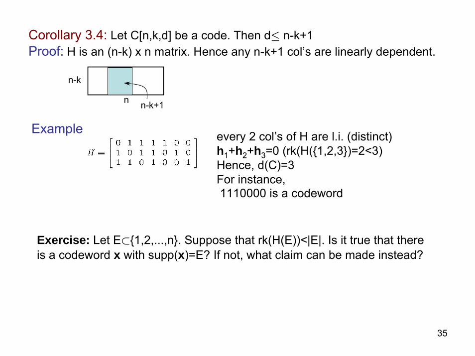
every 2 col’s of H are l.i. (distinct)h1+h2+h3=0 (rk(H({1,2,3})=2<3)Hence, d(C)=3 For instance,1110000 is a codeword

Example

Exercise: Let E⊂{1,2,...,n}. Suppose that rk(H(E))<|E|. Is it true that thereis a codeword x with supp(x)=E? If not, what claim can be made instead?

Corollary 3.4: Let C[n,k,d] be a code. Then d· n-k+1Proof: H is an (n-k) x n matrix. Hence any n-k+1 col’s are linearly dependent.

n-k

n n-k+1

36

Let C[n,k,d] be a code

Definition 3.2: A code C corrects an error vector e (under minimumdistance decoding) if for any x∈ C

d(x,x+e) < d(y,x+e) for all y∈ C\x( equivalently, w(e) < d(y,x+e) )

This definition holds for all codes, linear or not

We say that a code corrects up to t errors if it corrects all error vectors e ∈ F with w(e) · t

Correctable errors

37

Theorem 3.5: If d(C)≥ 2t+1 then the code corrects every combination of · t errors.

Proof: Let x,y ∈ C, wt(e)·t

2t+1 · d(x,y) · d(x,x+e)+d(y,x+e) · t+d(y,x+e), so

d(y,x+e) > t ≥ d(x,x+e)

Main result:

38

Let C be a code with distance 2t+1. All errors of wt · t are correctable.There are errors of weight >t that are not correctable (generally, but notalways, some errors of weight >t will be correctable)

For nonlinear codes, an error vector e can be correctable for sometransmitted codevectors x and not correctable for other codevectors

Example: C={0000,1110,1100} d=1x=0000 e=0010 correctablex=1110 the same e is not correctableDefinition 3.3: The set of correctable errors for a given code vector x is called the Voronoi region of x, denoted D(x,C)

39

Let C be a code with distance 2t+1. All errors of wt · t are correctableThere are errors of weight >t that are not correctable (generally, but notalways, some errors of weight >t will be correctable)

For nonlinear codes, an error vector e can be correctable for sometransmitted codevectors x and not correctable for other codevectors

Example: C={0000,1110,1100} d=1x=0000 e=0010 correctablex=1110 the same e is not correctableDefinition 3.3: The set of correctable errors for a given code vector x is called the Voronoi region of x, denoted D(x,C)

For linear codes the vector is either correctable or not for any transmitted vector of C (Voronoi regions of the codewords are congruent).

Theorem 3.6: The set of correctable errors is the same for any vector of a linear codeProof: Let e be such that d(x1+e,x1)<d(x1+e,x2) for all x2≠ x1

Suppose that d(x3+e,x3)≥d(x3+e,x4) for some x3,x4Then take y=x1+x3 so that x1=y+x3d(x3+y+e,x3+y)=d(x1+e,x1)≥d(x1+e,x4+y), where x4+y∈ C

Contradiction

40

Useful visualization

correctable errors ofweight ≥ t

correctable errors2t+1

41

Building geometric intuition: what do spaces F2n look like?

00

01

10

11

000

011

001010

110

111

101

100

Hamming distance = number of edges in a shortest path in thegraph from x1 to x2

42

00000

11111

5-dimensional Hamming cube

43

00000

11111

5-dimensional Hamming cube

44

8-dim hypercube projected on R3

45

Given a linear code C, let E(C) be the set of correctable errors

∀e∈ E(C) wt(e)<d(e,x) for all nonzero x∈ C

Given a vector x=(xn-1,...,x1,x0)∈ F, considera binary number X=∑i=0

n-1 xi 2i

Definition 3.5: Lexicographic order on F. x,y∈ Fx ≺ y if the binary numbers X<Y

defines a total order on F

00101 ≺ 01010 etc.(intuition: that’s how words are ordered in the dictionary, exceptfor us all the words are of equal length)

From here onward the codes are again binary.

46

Example: 00000 00001000100001100100 0010100110 001110100001001010100101101100011010111001111

10000100011001010011101001010110110101111100011001110101101111100111011111011111

increasing order

47

Standard array for a linear [n,k] code. Consider the quotient space F/C. Make a 2n-k x 2k table as follows: the first row is the codewords with 0 on left, otherwise ordered arbitrarilyRow i begins with the vector of the smallest weight ei that is not in rows 0,...,i-1. If there are several possibilities for ei, we take the smallest one lexicographically

0 x1 x2 .... x2k-1e1 x1+e1 x2+e1 ... x2k-1+e1e2 x1+e2 x2+e2 ... x2k-1+e2e3 x1+e3 x2+e3 ... x2k-1+e3...........................e2n-k-1 x

1+e2n-k-1 .... x2k-1+ e2n-k-1

Vectors 0,e1,...,e2n-k-1 are called coset leaders

Exercise: Cosets are equally sized, pairwise disjoint

Lemma 3.6 (Lagrange’s theorem) Let G be a finite group, F its subgroup.Then |G| is a multiple of |F|.

48

ENEE626 Lecture 4: Decoding of linear codes

Today's topics:

1. Maximum likelihood decoding of linear codesStandard array, syndrome tableinformation setsinformation set decoding

49

Theorem 4.1: E(C) = {coset leaders that are unique vectors of the smallestweight in their cosets}

Proof: Exercise In particular, all errors of weight · b(d-1)/2c are unique coset leaders.Generally, the question of locating all coset leaders is difficult.

Example 4.1:0000 000000 011101 101010 110111 Code0001 000001 011100 101011 110110 correctable error0010 000010 011111 101000 110101 0100 000100 011001 101110 110011 1000 001000 010101 100010 111111 1101 010000 001101 111010 100111 1010 100000 111101 001010 010111 0011 000011 011110 101001 110100 0101 000101 011000 101111 110010 not correctable0110 000110 011011 101100 110001 1001 001001 010100 100011 111110 1100 001100 010001 100110 111011 1111 010010 001111 111000 100101 1011 100001 111100 001011 010110 1110 100100 111001 001110 010011 0111 110000 101101 011010 000111

recover a p.-c.m

111000010100100010010001

H=

syndrome coset leader

50

Lemma 4.2: Let ei be a coset leader, y ∈ C+ei be a vector from thesame coset. Then Hei

T = HyT

The vector si=HeiT determines the coset uniquely. si is called

the syndrome (of this coset).

Definition 4.1: The Syndrome table is an array of pairs

(syndrome, coset leader) (see Example 4.1)

2n-k pairs, total size (2n-k)2n-k bits

Syndrome table

C[n,k]; H parity-check matrix

x∈ C HxT=(000...000)T

y ∉ C HyT=s

51

Maximum likelihood (ML) decoding(decoding by minimum distance).

Compute the syndrome of the received vector s=H yT

Decode y → y+e (coset leader)

Complexity of ML decoding O(n2k) time complexityor O(n 2n-k) space complexity to store the syndrome table

Constructing the syndrome table generally is difficult (exhaustive search). Becomes infeasible for large codes.

Error probability of ML decoding for a linear code on a BSC(p):

Pe(x)=P(decoding incorrect | x transmitted) does not depend on x (Thm. 3.5)

Pcorrect=∑i=0n Si pi (1-p)n-i

where Si= #(coset leaders of wt i that are correctable errors)

52

Definition 4.1: Suppose that a code C is used for transmission overa BSC. Let y ∈ {0,1}n be a received vector. The maximum likelihood decoding rule is a mapping ψ: {0,1}n a C such that

ψ(y)= arg max Pr[y|x] (if there are several solutions, declare an error)x∈ C

General definition of ML decoding

In the case of linear codes, this definition is equivalent to the definitionon the previous slide.

53

Information set decoding(Another implementation of ML decoding):

Let G[g1,g2,...,gn] be a generator matrix of a linear code gi – a binary k-column

Definition 4.2: A subset of coordinates i1,i2,...,ik is called an information set if the columns gi1

,gi2,...,gik

are linearly independent.

Definition 4.3: A code matrix is an M × n matrix whose rows are the codewords.

A subset i1,i2,...,ik forms an information set if the submatrix of the codematrix with columns with these indices contains all the possible 2k rows (exactly once each).

Lemma 4.3: A codeword can be recovered from its k coordinates in any information set.

54

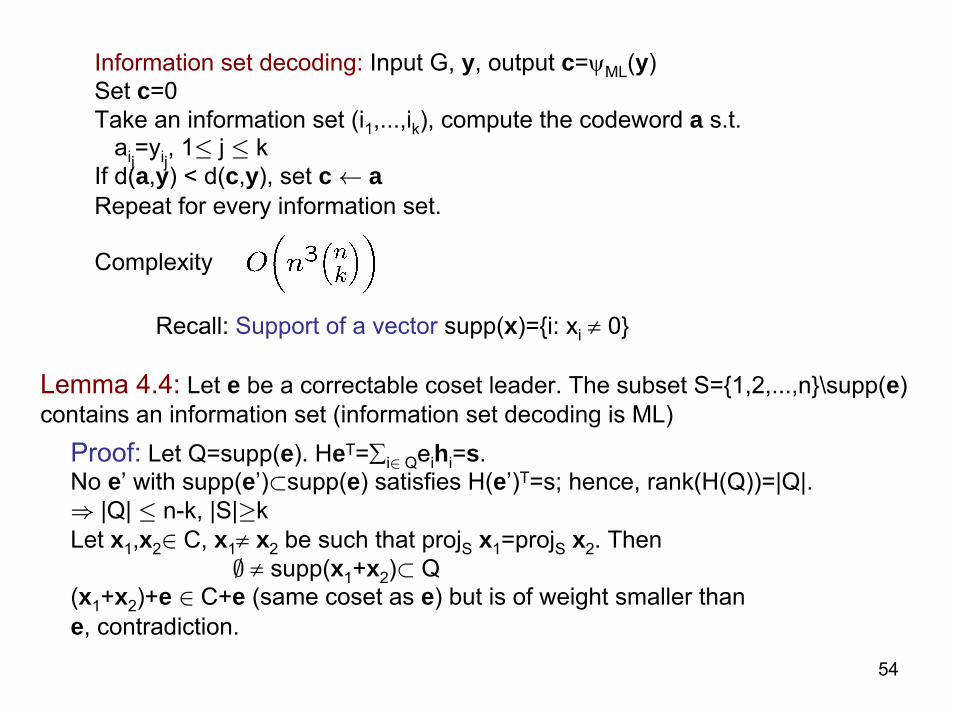
Information set decoding: Input G, y, output c=ψML(y)Set c=0Take an information set (i1,...,ik), compute the codeword a s.t.

aij=yij

, 1· j · kIf d(a,y) < d(c,y), set c ← aRepeat for every information set.

Complexity

Lemma 4.4: Let e be a correctable coset leader. The subset S={1,2,...,n}\supp(e) contains an information set (information set decoding is ML)

Recall: Support of a vector supp(x)={i: xi ≠ 0}

Proof: Let Q=supp(e). HeT=∑i∈ Qeihi=s.No e’ with supp(e’)⊂supp(e) satisfies H(e’)T=s; hence, rank(H(Q))=|Q|.⇒ |Q| · n-k, |S|≥kLet x1,x2∈ C, x1≠ x2 be such that projS x1=projS x2. Then

∅ ≠ supp(x1+x2)⊂ Q(x1+x2)+e ∈ C+e (same coset as e) but is of weight smaller thane, contradiction.

55

Example :

Subsets {1,2,3,4},{1,2,3,5}, {1,2,3,6},... are information sets

Subsets {3,7,8,9},... are not.

Generally it is difficult to find the number of information subsets of alinear code. Some indication of what to expect is given by consideringrandom matrices.

56

ENEE626 Lecture 5

Today's topics:

1. Rank of random binary matrices 2. The Hamming code; perfect codes3. The dual of the Hamming code (the simplex code)

57

Rank of random matrices

Theorem 5.1:

Given a random code, can we perform information set decoding?

58

Proof of part (a): Number of nonsingluar k x n matrices is

(2n-1)(2n-2)(2n-22)…(2n-2k-1)

In particular, let k=n. The probability that an n x n matrix over F2 is nonsingular equals

∏i=0n-1 (1-2-n+i)

One can prove that this product converges as n→∞. The limiting value is 0.2889.

N

59

H3[7,4,3] is a linear code with the p.-c.matrix0001111

H= 0110011 all nonzero 3-columns1010101

dim(H3)=4 , distance=31 011

G= 1 1011 1101 111

Syndrome table:syndrome leader

000 0000000 |Coset|=|H3|=16=2k

111 0000001 8 cosets ⇒ 128=27

110 0000010101 0000100 All single errors are correctable100 0001000 d ≥ 3=2x1+1011 0010000 010 0100000001 1000000

The Hamming code

60

Spheres in F:

Bt(x)={y∈ F: d(x,y)· t}

Vol(Bt(x)) denotes the volume of Bt(x) (number of points in the ball)

Proposition:

Volume does not depend on the center

61

Spheres of radius 1 about the c-words of the Hamming code are pairwise disjointvol(B1)=1+7=8total volume of spheres around the codewords=2k vol(B1)=16 x 8=128exhausts F2

7

Notation: C(n,M,d) a binary code of length n, size M, distance d

Definition 5.1: Perfect code C(n,M,2t+1)=spheres of radius t about the codewords contain all the poinrs of F2

n

Perfect codes are good but rare. Linear perfect codes are all known.

The Hamming code H3 is a linear 1-error-correcting perfect code.

Generalize: Hm[2m-1,2m-m-1,3] Hm=[all m-columns] Exercise: compute Gm.Decoding: correct 1 error. W.l.o.g. assume that we transmit x=0Transmit x, receive y=(00...010......00)

i

62

HyT=

hi1

= hi

columns ordered lexicographically: then hi gives the number ofthe coordinate in error. To decode, flip that coordinate.

No double, triple, ..., errors are correctable

63

HyT=

hi1

= hi

columns ordered lexicographically: then hi gives the number ofthe coordinate in error. To decode, flip that coordinate.

No double, triple, ..., errors are correctable

Message:to correct 1 errorwe need about log nparity check bits

Definition 5.2: Let C be a binary linear code. The dual code is

C⊥={x∈ F: ∀c∈ C (x,c)=0}

Properties: C⊥ is an [n,n-k] linear code generated by H, the p.-c.matrix of C.Distance of C⊥ =? Generally not immediate.

64

S2 S2

S2 S2

(Hm)⊥=Sm[2m-1,m,(n+1)/2=2m-1] called the simplex code

a very low-rate code with a very large distanceExercise: Is (111...111)∈ Hm?

Lemma 5.3: d (Sm )=2m-1

Proof: Induction on m

S3= the bar means negation 1→ 0, 0→ 1

00001111

inductionstep

65

The term “simplex”

000

011

001010

110

111

101

100

66

ENEE626 Lecture 6:

1. Weight distribution of the Hamming code.2. Code optimality, the Hamming and Plotkin bound3. The binary Golay codes4. Operations on codes.

67

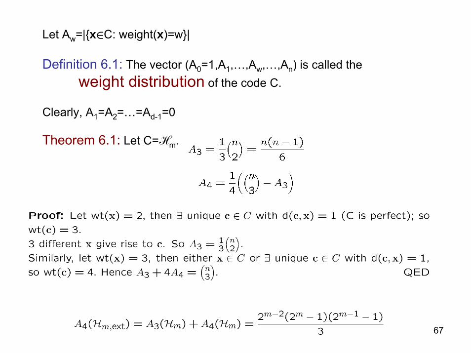
Let Aw=|{x∈C: weight(x)=w}|

Definition 6.1: The vector (A0=1,A1,…,Aw,…,An) is called the weight distribution of the code C.

Clearly, A1=A2=…=Ad-1=0

Theorem 6.1: Let C=Hm.

68

In principle, such recurrences can be used to compute the next weight coefficients in Hm, but there is a more efficient way (MacWilliams’ theorem, lect.7)

Interlude: The Hat Problemn=2m-1 people are given hats one each, either red or blue.At the same time they all walk into a room and see the hats of everyone else except their own. Then they guess simultaneously the color of theirown hats (if unsure they can pass). If those who do not pass all make a correct guess, the entire group win $1 each, otherwise they lose $1 each.

They can follow a pre-arranged strategy. Is there a strategy that willwin in more than 50% of color deals in the long run? (Was popular a few years ago; ran ran a front-page article)

69

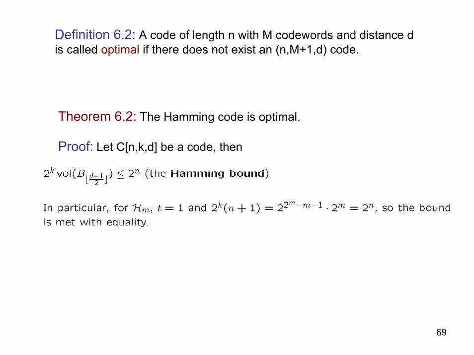
Theorem 6.2: The Hamming code is optimal.

Proof: Let C[n,k,d] be a code, then

Definition 6.2: A code of length n with M codewords and distance d is called optimal if there does not exist an (n,M+1,d) code.

70

Generally, if C is optimal, C⊥ is not always optimal. However, thisis true for Sm

Theorem 6.3 (the Plotkin bound) Let C[n,k,d] be a linear code. Then

In the [2m-1,m,2m-1] simplex code, 2d/(2d-n)=(n+1)/(n+1-n)=n+1=M

71

The Plotkin bound

It is also true for unrestricted codes, by the following argument.Let C(n,M,d) be a code. Compute the average distance between x,y∈ C.Let λi be the # of 1's in the ith column of the code matrix.

72

The Golay code: another binary perfect code

There exists a code G23[23,12,7] that corrects 3 errors

The only other binary linear perfect codes that exist are trivial:[n,n,1] (n ≥ 1), [2m+1,1,2m+1] (m≥1)Moreover, the only possibility for a nonlinear code to be perfect isthat its parameters coincide with the parameters of Hm

73

Operations on codes

Hm, ext[2m,2m-m-1,4]

[16,11,4]

Hm[2m-1,2m-m-1,3]

[15,11,3]

[2m-1,2m-m-2,4][15,10,4]

even-weight subcode

shorten by x1=0lengthen

deletingodd weights

append 115

overa

ll pa

rity ch

eck

punc

turing

74

Let C[n,k,d ≥ 2] be a linear code.Assume that the code (matrix) does not contain all-zero columns•Puncturing x a proj {1,...,n} \i x (projection)

C[n,k,d]→ C’[n-1,k,≥ d-1]

•Shortening C[n,k,d] → C’[n-1,k-1,≥ d]Lemma 6.4 (Lagrange’s theorem). A column in the code matrix contains 2k-1 0’s and 2k-1 1’s.To shorten C, take 2k-1 codevectors with a 0 in coord. i, removethe rest of C, delete that coordinate.

•Even weight subcode C[n,k,d=2t+1] → C’[n,k-1,d+1]delete all odd-weight codewords

•Adding overall parity check C[n,k,d=2t+1] → Cext[n+1,k,2t+2]Cext is called the extended code

Exercise. Let C be optimal. Is Cext also optimal?

•Lengthening C[n,k,d] → C’[n+1,k+1]add an overall parity check; append the vector 1n+1 to the basis of Cext

Operations on codes: Definitions

75

More ways to create a new code from known codes

|u|u+v| construction. Let A[n,k1,d1] and B[n,k2,d2] bebinary linear codes.

C=(|u|u+v|, u ∈ A, v ∈ B)

Lemma 6.5: C is a [2n,k1+k2,min(2d1,d2)] code

Proof: Let c ∈ C, c ≠ 0, v=0, then wt(c) ≥ 2d1On the other hand, if v ≠ 0, then

wt(c)=wt(u)+wt(u+v) ≥ wt(u)-wt(u)+wt(v)=wt(v) ≥ d2(triangle inequality wt(x+y) · wt(x)+wt(y) )

Example: Let A=Sm,ext, A[2m,m+1,2m-1]B[2m,1,2m]

Then C[2m+1,m+2,2m]=Sm+1,ext

76

ENEE626 Lecture 7: Weight distributions.The MacWilliams theorem

Weight distributions Bhattacharyya boundThe MacWilliams theorem Fourier transform

77

C a linear code, Aw =|{x∈C, wt(x)=w}|(A0,A1,…, An) weight distribution of a linear code C

Define the generating function of weights (the weight enumerator)A(x,y) = ∑i=0

n Ai xn-iyi

H3[7,4,3] i 0 1 2 3 4 5 6 7 A(x,y)=x7+7x4y3+7x3y4+y7

1 0 0 7 7 0 0 1S3[7,3,4] i 0 1 2 3 4 5 6 7 A⊥(x,y)=x7+7x3y4

1 0 0 0 7 0 0 0The weight enumerator of the code dual to C will be denoted by

A⊥(x,y); A⊥(x,y)=∑i Ai⊥ xn-iyi,

Weight distributions

78

Motivation to study weight distributions

2. Error detection. Suppose an [n,k,d] linear code C with weight enumerator A(x,y) is transmitted over a binary symmetric channel BSC(p) and used for error detection. Namely, the received vector is tested for being a code vector; if not, an error is declared. The probability of undetected error equals

Pud(C)=∑i=1n Aipi(1-p)n-i=A(1-p,p)-(1-p)n

For instance, let C be the [7,4,3] Hamming code H3.

1. The perfect code theorem from last lecture is proved using generalproperties of weight distriburions.

0.1 0.2 0.3 0.4 0.5

0.02

0.04

0.06

0.08

0.1

0.12

p

Pud(H3)

79

Motivation to study weight distributions

3. Error prob. of ML decoding. Suppose an [n,k,d] linear code with weight enumerator A(x,y) is transmitted over a binary symmetric channel BSC(p) and decoded by Max-likelihood (syndrome decoding). Let Pe(c) be the probability of error conditioned on transmitting the codeword c;

Pe(C):=2-k ∑c∈ C Pe(c)Then

Pe(C) · A( 1,2√p(1-p) )-1 (Bhattacharyya bound)

Proof. Suppose that the transmitted vector is 0 (does not matter);Let D(0) be the Voronoi region of 0. Let Pe,c’(0)=Pr(decode to c’|0)

N

80

Example: The [6,2,3] code C from Example 4.1

# correctable coset leaders S0=1; S1=6; S2=6weight distribution: A3=A4=A5=1Bhattacharyya bound: Pe(C)=γ3(1+γ+γ2), γ=2(p(1-p))1/2

Exact value: Pe(C)=1-((1-p)6+6p(1-p)5+6p2(1-p)4)

0.025 0.05 0.075 0.1 0.125 0.15

0.2

0.4

0.6

0.8

1

bound

exact

Pe(C)

p

Note: there are better bounds for Pe(C) for large p

81

Theorem 7.1:(MacWilliams) A⊥(x,y)=2-k A(x+y,x-y)So A(x,y)=2-n+k A⊥(x+y,x-y)

Example: compute the weight enumerator of H3 from the w.e. of S3:

A⊥(x+y,x-y)=(x+y)7+7(x+y)3(x-y)4=8x7+56 x4y3+56x3y4+8y7

=2-7+4 A(x,y)

Main result about the weight distributions

82

83

84

Nonbinary codes

Let C be a linear code of length n over Fq(means that x,y∈ C ⇒ ax+by∈ C)

For instance, F3={0,1,2} with operations mod 3

Definition 7.3. Let x=(x1,x2,...,xn) be a vector. The Hamming weightwt(x)=|{i: xi ≠ 0}|. The Hamming distance

d(x,y)=wt(x-y)

The weight distribution of the code C (A0,A1,....,An)

The weight enumerator A(x,y)=∑i=0n Ai xn-iyi

Definition 7.4: The dual code C⊥={y∈ (Fq)n : ∀x∈ C (x,y)=0} where (x,y)=∑i=1

n xi yi (operations in Fq)

Theorem 8.4 (MacWilliams): A⊥(x,y)= q-k A(x+(q-1)y,x-y)

Both proofs carry over to the general case