Instructional Module on

Semiconductor Processing

Raj Mutharasan Dept of Chemical Engineering

Drexel University

September 1997

Foreword

The purpose of this module is to introduce the transport phenomena topic, diffusion and transient diffusion, from the example of manufacture of integrated circuits. The primary instructional objective is the transport phenomena topic. The manufacturing processes provide a means to capture the interest and attention of the student. The manufacturing process is not intended to be comprehensive, but it is presented in sufficient detail so that the main ideas of manufacturing are discussed. This instructional module was used in a 3 hour course slot in CHE 319 Mass Transfer, a required course for all chemical engineering students taught at Junior level at Drexel in Fall, 1995. The review by students indicates that they found the manufacturing example very interesting. In fall of 1996, the multimedia was used in a course on fundamentals of transport phenomena taught to Civil and Materials Engineers at Drexel. Evaluation of this manufacturing segment showed very strong student response. The author highly recommends a 20-minute video summary of semiconductor processing prepared by Sematech, Corp. It is available free of cost from Sematech. The multimedia presentation of this topic provides an easy means of learning the background manufacturing material and the topic of diffusion. It is organized into the segments shown on the chart given on the next page. A multimedia CD is available which covers the topics of this teaching module. Any comments or suggestions may please be directed to

Raj.Mutharasan@CoE.Drexel.Edu.

Raj Mutharasan

September 1, 1997 September 10, 2000

1.1 Silicon

1.2 Oxidation

1.3 Lithography

1.4 Ion Implantation

1.5 Etching

1.0 Manufacturing

2.1 Conduction

2.2 Semiconductor

2.3 Doped Semiconductor

2.0 Semiconductors

3.1 Physics of Diffusion

3.2 Transient Diffusion

3.3 Diffusion Processing

Teacher

1: Transient Diffusion

2: Drive in Diffusion

Tutor

Diffusion Coeffcient

Dropant Profiling Conditon

Virtual Lab

Library

3.0 Diffusion

Semiconductor Processing

Semiconductor Processing

This document introduces you to an important processing technology in the manufacture of integrated circuits, namely diffusion processing. The overview segment will give you an overview of major manufacturing processes that are used in producing planar circuits. In the semiconductor properties chapter, you will be introduced to electronic behavior of semiconductor materials. The devices section illustrates the construction of three simple electronic devices, a resistor, a diode and a transistor. In the diffusion chapter you will learn principles and models used to manipulate time-temperature relationships for fabricating electronic devices. 1.0 Manufacturing Fabrication of integrated circuits starts with a thin slice of a silicon wafer, usually p-type silicon, 150 mm in diameter and 0.3 mm thick. On this wafer one can fabricate several hundred individual chips. Each chip may contain 10 to 20,000 components for a total of several million devices. The devices are resistors, diodes, capacitors and transistors of various types. The devices are fabricated by depositing controlled concentrations of dopants. Dopants are Group III and Group V elements that are introduced at concentration levels of parts per million. In most cases the depth to which the dopants are introduced into the wafer is less than a micron. These dimensions should give you the impression that the integrated chip is essentially a planar silicon crystal whose impurities or dopants are carefully created in specific small regions. In a sense, one can say fabricating an integrated circuit involves “planar chemical architecture”. A state-of-the-art silicon microchip contains 10 million devices within an area of about 1 sq. cm! The individual transistors are so small that one will need an electron microscope to see them. Figure 1 gives a scanning electron micrograph of a small area of an actual integrated circuit in which the line width is 0.5µm. Fig.2 shows a schematic cross-sectional view of a typical chip transistor. Materials typically used to make such a device are indicated on the figure. The thickness of the different layers is typically about 1 µm.

Fig. 1 A scanning electron micrograph of a small section of an integrated circuit. The line width is 0.5 µm.

Fig. 2 Cross sectional view of an IC transistor. AL is aluminum and is for making electrical connections. P refers to Group V rich region and N refers to

Group II rich region. The size of peripheral devices or components used in electronic systems has also been decreasing steadily over the years. For example, the thin film magnetic head (Fig.3) which is used to read and write hard disks is about the size of the period at the end of this sentence. These heads are fabricated using techniques similar to that used for the microchip fabrication. The tiny spiral around the head, as shown in Fig.3, is a thin film of electrical conductor obtained by evaporation of a metal.

Fig. 3 Enlarged view of a thin film magnetic head which is of the size of the tip of a needle.

Great manufacturing challenges were faced and overcome in making these tiny high quality devices and components with high reliability and reproducibility. Scientists and engineers are at work now to fabricate 256 to 512 million transistors on a microchip. We are stepping into a dimensional region where the action of only a few thousand atoms control the function of a device. Starting material for an integrated circuit is a silicon crystal in a wafer form. A wafer generally refers to thin flat silicon crystal; thickness is typically 300 µm and diameter is typically between 4 to 6 inches. Figure 4 shows a wafer being transferred for processing.

Figure 4 A silicon wafer being transferred automatically for processing

In the construction of integrated circuits, there are really two principle types of processing steps. First process type introduces desired chemical species into or on the wafer and the

second type is used to remove undesired material from the wafer. In the process that introduce dopants (that is Group V and III elements), the principal methods used are ion implantation for deposition and diffusion for profiling the dopant. Other methods include oxidation, chemical and physical vapor deposition. Processes used to remove material from the wafer surface are vapor phase etching, chemical etching and dissolution. We rely on a technique called lithography for the introduction of dopants at desired locations on the wafer and removal of undesired material. Manufacture of microchips involves repeating the above two types of processing steps several times, until we fabricate a complete device, such as a transistor. As many as 200 steps may be needed to fabricate a chip which may have multiple layers. To get our final circuits, we need to wire up the arrays of components. The components are so small, their dimensions are in the micrometer range. We deposit a thin layer of aluminum film, by evaporative technique, on the surface of the wafer. Selective etching is done to remove unwanted aluminum films leaving a desired circuit pattern Finally a thin protecting layer, such as silicon dioxide, on the top of the circuits is introduced to protect them from the environment. The wafer is then diced into individual chips simply by a sawing operation. The chips are then packaged and mounted on a suitable platform, such as chip carriers or lead frames. The manufacturing process is divided into five major segments, silicon, oxidation, lithography, ion implantation and etching. 1.1 Silicon Most silicon crystals used in building integrated circuits are grown by Czochralski method. This is a simple liquid to solid monocomponent transformation process. The crystal is grown from a seed crystal which is drawn from silicon melt maintained at a temperature slightly higher than silicon melting point. The seed crystal enables orientation of the crystal growth axis. The silicon crystal can be as large as four feet and as thick a diameter as six inches. The silicon ingot or crystal is called a boule and has a gray shiny texture. The crystal is cut into thin slices of about 300 µm wafers, polished and etched to ensure that the faces of water are parallel and free from contamination.

Figure 5 A Finished Wafer 1.2 Oxidation Formation of silicon dioxide layer is one of the most frequently used steps in integrated circuits manufacture. Silicon dioxide is an electrical insulator and is usually created in situ by thermal oxidation. The SiO2 layer is used as a mask during dopant diffusion, as a junction passivation, as an insulating field oxide and as a gate dielectric. Dry oxidation is performed by exposing silicon to oxygen at a bout 1000 C. Oxidation rate is more rapid if moisture is mixed in with oxygen. This process is called wet oxidation. Dry oxidation produces high quality thin oxide layers of 0.05 µm while wet oxidation produces thick oxide layers of 0.5 µm.

Fig 6 A stack of wafers being loaded into furnace for oxidation

Oxidation takes place at silicon-silicon dioxide interface. Oxygen must diffuse through SiO2 layer to this interface to react. Because SiO2 is a barrier to oxygen diffusion, growth rate of SiO2 decreases with time. For initial processing steps a thickness of 500 A or 0.05 µm is adequate and is usually grown within 30 minutes at 900 C in oxygen atmosphere. 1.3 Lithography Photo lithography is a process in which wafer is coated with a light sensitive polymer called photoresist. . Polyisoprene is an example of a commonly used photoactive agent.

Fig 7 Photoresist is spray applied to wafer A mask is used to expose selected areas of photoresist to UV light. The UV light induces polymerization in the exposed photoresist. UV causes it to cross link rendering it insoluble in developing solution. Such a photoresist is called a positive photoresist. A negative photoresist shows an opposite behavior. That is exposure to UV makes the photoresist soluble in developing solution.

1.4 Ion Implantation and Diffusion Dopant atoms are deposited on wafer surface and then diffused in at high temperature. The diffusion time and temperature as well as dopant concentration on surface must be controlled to obtain desired dopant profile.

Fig 8 Ion Implantation. Picture on right shows approach of ions toward wafer. Current approach to doping is ion implantation. Ions of dopant atoms are accelerated to a high velocity in an electric field and impinge on target wafer. The ions penetrate through the oxide layer and enter into silicon. Penetration depths of 500 to 5000 A are easily achieved. Penetration depth depends on size of ion and energy applied. The ions do not penetrate the photoresist layers which are typically 10,000 A thick. By manipulating the acceleration voltage, the average implantation depth can be precisely controlled. The dopant concentration can be carefully controlled by monitoring implantation current. Ion implantation technique enables us to introduce dopants at low temperature and it allows the incorporation of a variety of atoms. Disadvantage being slow speed and cost. During high velocity impact of dopant atoms, the underlying crystal is damaged and a post implantation anneal at 800 C for 30 minutes is often required to remove the created defects, prior to profiling dopant concentration by a diffusion step. 1.5 Etching Process that follows immediately after photolithography step is the removal of material from areas unprotected by photoresist. This process must be selective; that is SiO2 is removed while leaving photoresist and silicon intact. It must also be anisotropic; that is etching should be in one direction only.

Fig 9 Physical Etching Two types of etching processes are used in practice; namely, chemical and physical etching. In purely chemical etching material is removed by dissolution which is highly selective but not anisotropic. In purely physical method material is removed by bombardment of high energy ions which is inherently anisotropic but unselective. As an example, SiO2 which is used as a mask for drive in diffusion is removed by exposure to hydrogen fluoride. Hydrogen fluoride reacts with SiO2 to form volatile SiF4 which is swept away by inert argon gas. 2.0 Semiconductor Properties In this section you will learn about basic physics of conduction, conduction behavior of pure semiconductors and behavior of doped semiconductors. At the end of this section, you will be able to calculate dimension and concentration parameters of a semiconductor resistor. 2.1 Conduction Conduction occurs in a solid if mobile charge carriers are available. In metals such as copper the atoms are arranged in a systematic manner called crystals. The valence electrons are loosely bound to the nucleus creating what is called an "electron sea". These free floating electrons are more precisely called “delocalized” electrons are responsible for conduction, because they are able to move thus enabling carrying of charge. When an electric field of E volts/m is applied, electrons accelerate and move opposite to the direction of applied field crating current flow. Electron is a negative charge carrier. It carries a charge of 1.6 10-19 Coulombs, abbreviated by the symbol C. Note also that charge is integral of current over time; hence C is dimensionally Amp-seconds, or simply denoted as A-s. We also have a positive charge carrier called electron hole, abbreviated by the symbol h. It is described as the absence of an electron and therefore has a positive charge. Its charge carrying capacity is exactly equal to that of an electron except for its sign. e: - 1.6 x 10-19 C h: + 1.6 x 10-19 C Conductivity of a material depends on the number of charge carriers present and their mobility under an applied electric field. That is Conductivity = {mobility } { number density of carriers} {charge carried by each}

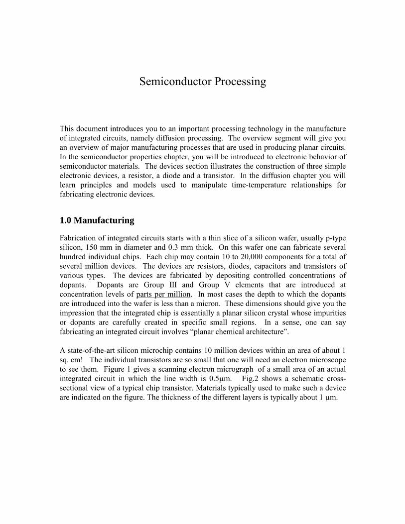
The above can be expressed as σ = m n q where σ is conductivity, n is number density and q is the magnitude of charge carried by each electron or hole. The parameter, µ, is the charge mobility and is the velocity of a unit charge carrier when subjected to unit applied field, E. That is

µ = Ch arg e Velocity

Applied Electric Field ⇒

m / sV / m

⇒ m2

V − s

The units of conductivity is therefore given by

Units of σ = m2

V −s

#m3

A − s( ) ⇒ Ohm−1 m−1

In this relationship, we have replaced V/A with ohm. Inverse ohm is called Siemen and it is common to refer to the units of ohm-1 m-1 as simply Siemens per meter. Recall that resistance of a conductive element is inversely proportional to area of conductive path and directly proportional to conductor length. This can be expressed mathematically as

R = ρLA

where the proportionality constant is indicated as ρ. The term, ρ is resistivity and has the dimensions of ohm-m. Inverse of resistivity is conductivity, σ. That is

R = 1σ

LA

Let us now examine how s of semiconductors can be systematically altered and how one would determine the concentration of dopants needed to obtain a desired level of conductivity. 2.2 Semiconductor Crystal structure of silicon or germanium follows a tetrahedral pattern with each atom sharing one valence electron with each of four neighboring atoms. Let us examine this arrangement in two dimensions, for ease of representation. At low temperature most of the electrons are confined to the covalent bond region resulting in very low conductivity. At room temperature, a few electrons would have acquired enough energy to “jump”: out of the valence band and enter into the conduction band. That is a few electrons that are

delocalized are free to “float” around as in metallic materials. It is useful for you to think about the conduction band electrons as mobile while covalent bond electrons as essentially immobile and localized. Now, the absence (or vacancy) of an electron in one of the covalent bond in the silicon lattice will create a local positive charge called “electron hole”. On the other hand, presence of conduction band electrons, over and above that is needed to satisfy covalent bonds will create a local negative charge. You will note that in a pure silicon crystal, we will have exactly the same number of conduction electrons ( that is mobile electrons) as holes. If we apply an electric potential to this crystal, the electrons will migrate toward the positive electrode and the holes will migrate towards the negative terminal. The conductivity can be calculated from the relationship introduced in the last section.

σ = m n q

Since there are two charge carriers, namely e and h, the above equation is modified to include both electrons and holes. That is,

σ = µnn + µpp( ) q In the above equation n and p refer to number density of negative and positive charge carriers respectively. The mobility of holes tend to be lower than that of electrons. Mobility of electrons and holes in pure silicon crystal at room temperature are given below.

Mobility of electrons = µn = 0.135 m2

V − s

Mobility of electrons = µp = 0.048 m2

V − s

Since the number of conduction electrons and holes are created simultaneously in a pure Si crystal, we can simplify the above equation by substituting ni for n and p. The conductivity relationship is therefore further simplified as

σ = ni µn + µp( ) q For pure silicon at room temperature, ni is about 1.5 x 1016 per m3. Let us consider a simple example.

Example: 1 Calculate the resistance of a 10 µm diameter cylinder of pure Si of 100 µm length at room temperature. Density of Si is 2.33 x 106 g/m3. Solution: First calculate conductivity of Si using reported mobility values for e and h. That is:

σ = ni µn + µp( ) q ⇒ (1.5 x 1016) • (0.135 + 0.048)• (1.6 x 10−19 )

= 4.4 x 10−4 S/ m

Next, calculate resistance:

R =

1σ

LA

⇒ 1

4.4 x 10−4 S/ m •

100 x 10−6 mπ4

10 x 10−6( )2 m2

= 2.9 x 109 ohms

2.3 Doped Semiconductors From the previous section we found that the number of charge carrying species is extremely small in the case of pure semiconductors -- it was of the order of 1016 #/m3. That is, only one out of one trillion Si atoms loses its electron to the conduction band. Doping is a process by which we can increase structurally the number of conduction electrons or conduction holes in the Si crystal. If we were to increase the number of electrons by say 1016 #/m3, conductivity will double. Although 1016 charges per m3 seems large, it turns out to be a very small concentration, of the order of one part in a trillion. How do we then introduce conduction electrons or holes. It can be done by forcing into a silicon crystal another atom that has more number of valence electrons. An example of this is phosphorous. which is pentavalent. When we introduce trivalent atoms such as Boron, we create holes or positively disposed semiconductor, also called p-type semiconductor. When phosphorous is introduced we create negatively disposed semiconductor because of excess electrons and is called n-type semiconductor. You will note that Group III elements are a source of p-type dopants and n-type semiconductors are created using Group V elements. Another term commonly used is donor and acceptor semiconductor. n-type is called donor because of its ability to “donate” electrons while p-type is called acceptor because of its propensity to “accept” electrons.

Group V elements = Forms Donor Semiconductor = n-type Semiconductor

Group III elements = Forms Acceptor Semiconductor = p-type Semiconductor

When we introduce dopants to an intrinsic semiconductor, practically all donor or acceptor atoms generate electrons or holes in proportion to their concentration in Si. This is because intrinsic concentration of free electrons or holes in pure Si crystal is so small, we can make the above approximation without any loss in accuracy. Let us consider an example.

Example 2: What concentration of Boron is needed to increase Silicon conductivity from 4.4 x 10-4 S/m to 100 S/m. Solution: Since B is a Group III element, it will introduce holes into Si crystal. Let the concentration of holes be p. Mobility of p in Si is 0.048 m2/A-s. Use conductivity equation to determine desired value of p.

σ = µnn + µpp( ) q

The number of negative charges in the silicon will be very small compared to holes introduced by Boron doping. Hence, we will set n = 0 in the above equation. Substituting values, we get:

100 = (0) (µn ) + (p) (0.048)[ ] • (1.6 x 10−19 )

⇒ 1.3 x 1022 ch arg es/ m3

Number of Si atoms per unit volume is 5 x 1028 # / m3

Therefore, B concentration is = 1.3 x 1022

5 x 1028 ⇒ 0.26 x 10−6

That is, about 0.3 parts per million Boron is needed !

The above example shows that to increase conductivity by nearly a million fold, we need B concentration of 0.3 ppm! In Example 1, we found that resistance of pure silicon rod was 2.9 x 109 ohms. If it was modified with 0.3 ppm B, its resistance would decrease to 12,760 ohms. In the next section, we will learn how to determine conditions needed (temperature and time) to achieve the above desired level of Boron concentration. 3.0 Diffusion Diffusion is the transport mechanism by which dopant atoms are distributed in the silicon crystal to the derived depth and desired concentration. In an earlier section we introduced dopant atoms on the surface of the wafer using a vapor deposition method (Fig.3-1a) or by ion implantation technique (Fig 3-1b).

Dopant

Si Wafer

Fig 1a

Dopant

Si Wafer

Fig 1b

SiO2

Figure 3-1 Two Geometry’s of Dopant Diffusion

You will note that in the case of CVD method, the SiO2 layer is removed prior to CVD deposition while in ion implantation method, dopant atoms are implanted through the oxide layer. In the diffusion step, that follows, profiling the dopant concentration is accomplished. Ideally, the dopant will penetrate to a desired distance, called junction depth, Xj below the wafer surface and will be of uniform concentration. In this chapter you will be first introduced to physics of diffusion in solid state, followed by the

development of a diffusion model to describe evolution of dopant concentration profile in a thermal diffusion process. 3.1 Physics of Diffusion Two major theories of diffusion have been proposed. These are continuum theory of Fick and the atomistic theory of defects and vacancies. Let us consider Fick’s approach first. Fickian theory states that flux of a species across a plane is proportional to concentration gradient. That is, as illustrated in Fig 3-2, the number of atoms of A that

X

Y

Z Plane X

High CA Low CA

Figure 3-2 Plane of Diffusion. Diffusion paths are not straight lines. Diffusion may occur in a direction opposite to concentration gradient at molecular scales, but the overall diffusion will occur from high to low concentration.

will cross the X-plane per unit area and per unit time in the direction of X is proportional to the first derivative of concentration. That is

J Ax is proportional to ∂CA∂x

(3-1)

We use partial differential to express concentration gradient because concentration in general can vary with the other directions y and z. Flux in X- direction, JAx has the units of number of atoms of A diffusing per unit area (m2) per unit time (s). The above can be written as an equation by introducing a proportionality constant called diffusion coefficient, D. That is

J Ax = D ∂CA∂x

(3-2)

If x is in measured in meters and concentration, CA is in number of atoms per cubic meters, the diffusion coefficient will have the units of square meters per second (m2 s-1) If we limit the discussion to only one dimensional transport, which means that concentration of A does not change in y and z directions in the example we are considering, we can convert the partial differentials to total differentials, and the above equation becomes

J Ax = D dCAdx

(3-3)

Let us consider the region in which A is diffusing as consisting of pure B. (In our applications, B will be silicon.) We can mathematically indicate this by labeling the proportionality constant as DA diffusing in B, and for short we will use the symbol DAB. (Some use the notation, DA-B. to indicate the same). That is, the diffusion equation now takes the form

J Ax = DAB dCAdx

(3-4)

If concentration of A decreases along x from left to right as shown in the figures, we would say that A is diffusing from left to right, because diffusion occurs from a region of higher concentration to a region of lower concentration. This is analogous to heat flowing from higher temperature to lower temperature and fluid flowing from higher pressure to

lower pressure. In the present example, dCAdx

will be negative because A decreases from

left to right. In order to preserve our common sense understanding of diffusion direction (similar to heat flow direction), we would have to include a negative sign on the right hand side. That is

J Ax = − DAB dCAdx

(3-5)

In this form, we have defined Fickian theory of diffusion (stated earlier descriptively) in a precise mathematical form. If we were to consider diffusion in three dimensions, we would write the above equation as

JA = − DAB ∂C A

∂x i +∂CA

∂y j +∂C A

∂z k

(3-6)

or simply, JA = − DAB ∇ CA

where ∇ is the gradient operator and i, j and k are unit vectors in s, y and z. In this form concentration is allowed to be a function of x, y and z. Although the general 3-dimensional form is more complete, in many situations one dimensional form is adequate to describe process behavior. Let us now consider the one-dimensional model. The diffusion coefficient can be considered constant when A is diffusing through essentially pure B. That is, A is present in B in dilute concentrations. As we stated earlier, the diffusion coefficient does depend on the nature of medium in which the diffusion occurs. In fact this is the reason why we included the subscript AB on the diffusion coefficient. It is therefore not a surprise that DAB will vary with concentration of B. In gas phase, average distance between molecules are so far apart compared to liquid and solid, and compared to distances over which the inter-molecular forces of attraction and repulsion occur that we usually approve DAB as a constant in gas phase. In liquids and in solids, and the current application in semiconductor processing, we cannot make such an approximation without some loss in accuracy. 3.2 Diffusion Processing Previously we saw how dopant atoms are deposited on a silicon wafer. The dopant must be profiled to a desired depth in the wafer. One method of achieving profiling is by diffusion. Profiling requires heating the wafer and holding it at a specific temperature for a fixed period of time so that desired diffusion depth and dopant profile are achieved.

The first step of depositing dopant is called “pre-deposition” and the subsequent profiling is called “drive-in diffusion”. In pre-disposition , wafer is exposed to dopant containing gas in a high temperature environment. A constant dopant concentration is established on the exposed wafer surface. The goal of the predisposition step is to diffuse a small amount of dopant into the surface. The dopant is deposited on the surface continuously. If we now heat the wafer, the dopants will diffuse into the depth of the wafer, as well as out of the wafer. The profile of the dopant will change with time as shown in Figure 3-3.

0.000.100.200.300.400.500.600.700.800.901.00

0 0.5 1 1.5 2Depth in µm

d Increasingi

Figure 3-3 Dopant Profiles without sealing SiO2 layer.

Note that the concentration profile exhibits a sharp gradient, especially in the surface region. That is, concentration profile of dopant changes quite drastically with depth near the top of the wafer. Since introduction of each dopant atom generates a conductive species (a delocalized electron or a conduction hole), strong variations in concentration of dopant species will result in undesirable conductivity variations. Therefore, the wafer is further processed to obtain uniform dopant concentration. This is achieved by sealing the top

0.000.100.200.300.400.500.600.700.800.901.00

0 0.5 1 1.5 2

Depth in µm

Nor

mal

ized

con

cent

ratio

n

Increasing time

Figure 3-4 Dopant Profiles with sealing SiO2 layer. surface by growing a thin impervious layer of silicon oxide by oxidation. Because SiO2 layer prevents diffusion of dopant out of the top wafer surface, the dopant profile tends to

be flatter in the surface region. With SiO2 sealing layer, the nature of dopant profile change is shown in Figure 3-4. Compare the two profiles. One has a region of nearly constant dopant concentration (and hence conductivity) while the other has region of variable conductivity. Profiling with a sealing SiO2 layer is called drive-in diffusion. Next, we will examine mathematical relationships which will enable us to calculate diffusion time and temperature. Mathematical Modeling of Pre-Deposition Consider the pre-deposition step. The wafer is placed in an atmosphere in which dopant atoms are deposited on the surface by a gas that bears the dopant atom. Let the concentration of dopant A at the surface be CAs, given in atoms per cm3. The surface concentration (Cas) will remain constant during the pre-deposition step. The value of CAs depends strongly on temperature and on the dopant. For example, Boron’s value at 1223 K is 4.5 x 1020 atoms/cm3 and increases by about 35% as temperature is increased to 1423 K. Referring to Figure 3-5, consider a control volume of thickness dx and length and depth of unit distance.

X dx

Dopant, A

Diffusion in

Diffusion out

XX + dx

CAs

CA0

Fig 3-5 Diffusion Geometry The amount of A diffusing in at x is given by Fick’s Law,

− DAB (∆x • 1) ∂CA∂x x

and the amount of A diffusing out at x+Dx is

− DAB (∆x • 1) ∂CA∂x x+dx

The difference is accumulated within the control volume and is given by

− DAB (∆x • 1) ∂CA∂x

x − − DAB (∆x • 1) ∂CA

∂x

x+dx = ∂(∆x • 1• 1• CA )

∂t

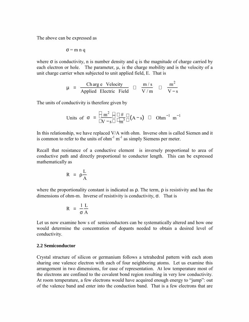
Dividing the above by dx and then taking the limit as dx goes to zero, one gets the classical one dimensional transient diffusion equation shown below.

DAB ∂2CA∂x2 = ∂CA

∂t (3-7)

The above is a partial differential equation whose solution depends on the boundary conditions we impose. When we maintain a constant surface concentration of CAs during pre-deposition, the following boundary values are applicable.

CA = CAs at x = 0, for all t ≥ 0CA = CA0 at x → ∞, for all t ≥ 0CA = CA0 for all x ≥ 0, at t = 0

(3-8)

The first two equations above state that the surface concentration and concentration far-far away from the surface are constant values. The distance of infinity is not to be interpreted literally; instead one visualizes any distance farther than the region wherein concentration changes as being infinite distance. For example, in Figure 3-3 and 3-4, a distance of 2 µm can be treated as infinite distance within the time frame considered. The third condition imposed above is the initial condition, namely the concentration profile within the wafer before the pre-deposition was initiated. Here the statement is to be taken as the wafer having a constant dopant concentration of CA0. In many practical applications, CA0 will be zero. Here, we will use a variable in our formulation to maintain a greater level of generality. The solution to Equation (3-7) subjected to boundary conditions in (3-8) is given below.

AC − ASCAOC − ASC

= erfx

2 ABD t

(3-9)

The abbreviation “erf” refers to error function. Error function of a variable y is defined as:

erf (y) = 2π

e−z 2 dz

0

y

∫ (3-10)

As shown in Figure 3-6, error function increases monotonically from 0 to 1 as its argument increases; it is essentially 1 when argument is 2. Error function is an odd

function, meaning that its value when its argument is negative is negative. that is: erf(-y) = - erf(y).

0.000.100.200.300.400.500.600.700.800.901.00

0.0 0.3 0.5 0.8 1.0 1.3 1.5 1.8 2.0y

erf (

y)

Figure 3-6 Error Function Values

Mathematical Model of Drive-In Diffusion In the pre-deposition step we found that the concentration profile of dopant A was expressed as an error function. See Eqn (3-9). If the time period of pre-deposition is t1, the amount of dopant that was deposited will equal to:

Dopant Deposited = (Area of Deposition) (Flux of A at x = 0) dt

0

t1

∫ = A J A x=0 dt

0

t1

∫ (3 −11)

= (cm2 ) • atomscm2 • s

• s( ) ⇒ atoms

Flux of A at x = 0 is obtained from Fick’s Equation:

J A x = 0 = − DAB ∂CA∂x x = 0

(3 −11a)

We know the concentration profile of A at the end of pre-deposition step, given by Eq (3-9). It can be rearranged to express dopant concentration explicitly as

CA = CAs − CAs − CA0( ) erfx

2 ABD t

(3 −11b)

We can now take partial derivative of the above to obtain flux at x = 0.

J A x=0 = − DAB

∂∂x

CAs − CAs − CA 0( ) erf x2 ABD t

x=0

= CAs − CA0

π tDAB

(3-12)

Note that flux at the interface decreases with square root of time and is directly proportional to concentration difference and square root of diffusion coefficient. The amount of dopant deposited can now be calculated by substituting the above in Eq (3-11). That is:

Dopant Deposited = A CAs − CA0

π tDAB0

t

∫ dt ⇒ 2 A

π CAs − CA0( ) DAB t

It is conventional to report amount of dopant deposited per unit area rather than the total amount deposited. Therefore dividing the above by the area term, we get the following design relationship:

Dopant per unit area ⇒ β =2π

CAs − CA0( ) DAB t in atomscm2 (3-13)

If pre-deposition is carried out for a time period of t1 and at a temperature of T1, then “beta” is calculated by

β =2π

CAs − CA0( ) D1 t1 (3-14)

where D1 is diffusion coefficient at T1. Mathematical Model of Drive-In Diffusion - Dopant Profiling After pre-deposition, the wafer is usually placed in a furnace at a higher temperature, first to grow a sealing silicon dioxide layer and then to achieve dopant concentration profiling. Let the diffusion coefficient at this higher temperature, T2 be D2. The diffusion of dopant during this phase of operation is also described by an equation similar to Eq (3-7 ) with the modification given below. Subscript A is dropped in all further developments. That is: C will refer to concentration of A.

D2 ∂2C∂x2 =

∂C∂t

(3-15)

At the top surface, x = 0, flux of A will be zero because of the sealing oxide layer. We express this condition mathematically as the gradient of C is zero. Recall that flux is directly proportional to the gradient. That is

∂C∂x

= 0 at x = 0, for all t ≥ 0 (3-15a)

Far away (more than 1 or 2 microns) from the top surface, we expect concentration of A not to change during the course of drive-in diffusion. This expressed as:

C = C0 at x → ∞ for all t ≥ 0 (3-15b) The initial condition is the profile that existed at the end of pre-deposition step, and is given by Equation (3-11b) and is given below for a pre-deposition time of t1 and temperature of T1.

C = Cs − Cs − C0( ) erfx

2 1D 1t

(3-15c)

The solution to Eq (3-15) with the boundary conditions stated above is given by

C − C0Cs − C0

= 2π

D1t1D2t

0.5

exp −x2

4D2t

(3-16)

where t is drive-in diffusion time. In many applications, dopant initial concentration, C0 is so small in comparison to the dopant concentration introduced that we can set it to zero. Further, if time is set to drive-in diffusion time, t2, then the above simplifies to:

CCs

= 2π

D1t1D2t 2

12

exp − x2

4D2t2

(3-17)

The junction depth, xj is the distance at which concentration of dopant is approximately equal to C0. Setting C to C0 in the above, and rearranging junction depth can be expressed as:

x j = 4D2t2 ln2π

CsC0

D1t1D2t 2

12

12

(3-18)

Example 3 A junction in silicon is made by doping with Boron using pre-deposition followed by drive-in diffusion.

a) Five minutes at 1100o C are required to deposit the dopant. At what distance from the surface is the concentration of Boron raised to 3 x 1018 atoms/cm3. Assume that silicon is pure. b) How much boron ( per cm2 of silicon surface) will have been taken up by the silicon during the deposition step ?

c) To prevent loss of Boron during drive-in step, surface is masked with silica. Now calculate tie required to achieve a Boron concentration of 3 x 1018 atoms/cm3 at a depth of 6 microns. Temperature of operation is: 1150 C

Part a Since silicon is pure, C0 = o. Time of diffusion = t = 5 minutes Desired concentration = C = 3 x 1018 atoms/cm3 Diffusion Coefficient of B at 1100 C is (from Hand Book) = D = 5.8 x 10-2 µm2/h Surface concentration of B at 1100 C is (from Hand Book) = Cs = 5.1 x 1020 atoms/cm3 The relevant diffusion equation is:

C − sC0C − sC

= erfx

2 D t

Substitute the knowns in the above.

3 x 1018 − 5.1 x 1020

0 − 5.1 x 1020 = erf x

2 5.8 x 10−2( ) 560

The unknown, x is obtained by determining the referring to the error function graph. Solution: x ~ 0.27 µ m. Part b The amount deposited is calculated using the formula given in Equation (3-13)

β = 2π

CAs − CA0( ) D1 t1

β = 2π

5.1 x 1020 − 0( ) 5.8 x 10−2

104

5

60

β = 4 x 1015 atomscm2

Part c Time required for the drive-in diffusion step can be obtained from Equation (3-17)

CCs

= 2π

D1t1D2t 2

12

exp −x2

4D2t2

Here C = 3 x 1018, x = 6 µm, Cs = 5.1 x 1020

Diffusion Coefficient of B at 1100 C is (from Hand Book) = D1 = 5.8 x 10-2 µm2/h Diffusion Coefficient of B at 1150 C is (from Hand Book) = D2 = 1.6 x 10-1 µm2/h time, t1 = (5/60) h Substituting in the above:

3 x 1018

5 x 1020 = 2π

0.058• (5/ 60)(0.16) • (t2)

12

exp −62

(4) (0.16) (t 2)

Solving, t2 = 203 h (this is not a typical drive-in diffusion time, which is typically an hour; the depth of 6 microns is much larger than a typical practical need of about 1 micron.)