InstituteofComputerGraphicsandAlgorithms TUWien,Vienna,Austria · A feasible solution S (also called schedule) to SI-PTPSP is a vector of values S a 2 T a assigning each activity

Algorithms and Complexity Group | Institute of Computer Graphics and Algorithms | TUWien, Vienna, Austria

Technical Report AC-TR-17-001first version: March 2017updated: September 2017

An Iterative Time-BucketRefinement Algorithm for aHigh ResolutionResource-ConstrainedProject SchedulingProblemMartin Riedler, Thomas Jatschka, JohannesMaschler, and Günther R. Raidl

www.ac.tuwien.ac.at/tr

An Iterative Time-Bucket RefinementAlgorithm for a High Resolution

Resource-Constrained Project SchedulingProblem

Martin Riedler, Thomas Jatschka,Johannes Maschler, and Gunther R. Raidl

Institute of Computer Graphics and Algorithms, TU Wien, Austria

{maschler|riedler|raidl}@ac.tuwien.ac.at, [email protected]

We consider a resource-constrained project scheduling problem originatingin particle therapy for cancer treatment, in which the scheduling has to bedone in high resolution. Traditional mixed integer linear programming tech-niques such as time-indexed formulations or discrete-event formulations areknown to have severe limitations in such cases, i.e., growing too fast or havingweak linear programming relaxations. We suggest a relaxation based on par-titioning time into so-called time-buckets. This relaxation is iteratively solvedand serves as basis for deriving feasible solutions using heuristics. Based onthese primal and dual solutions and bounds the time-buckets are successivelyrefined. Combining these parts we obtain an algorithm that provides goodapproximate solutions soon and eventually converges to an optimal solution.Diverse strategies for performing the time-bucket refinement are investigated.The approach shows excellent performance in comparison to the traditionalformulations and a metaheuristic.

Keywords. Resource-Constrained Project Scheduling, Time-Bucket Relaxation, MixedInteger Linear Programming, Matheuristics, Particle Therapy

1 Introduction

Scheduling problems arise in a variety of practical applications. Prominent examples arejob shop or project scheduling problems that require a set of activities to be scheduledover time. The execution of the activities typically depends on certain resources of lim-ited availability and diverse other restrictions such as precedence constraints. The goal is

1

TechnicalReportAC-TR-17-001

to find a feasible schedule that minimizes some objective function like the makespan. Incertain cases, scheduling has to be done in a very fine-grained way, i.e., in high resolution,using, e.g., seconds or even milliseconds as unit of time.

Classical mixed integer linear programming (MILP) formulations are known to strug-gle under these conditions. On the one hand, time discretized models provide stronglinear programming (LP) bounds but grow too quickly with the instance size due to thefine time discretization. Event-based and sequencing-based models on the other handtypically have trouble as a result of their weak LP bounds.

In the following, we focus on problems with a large, very fine-grained scheduling hori-zon and consider a simplified scheduling problem arising in the context of modern particletherapy used for cancer treatment. The problem is motivated by a real world patientscheduling scenario at the recently founded cancer treatment center MedAustron locatedin Wiener Neustadt, Austria1. The tasks involved in providing a given set of patientswith their individual particle treatments shall be scheduled in such a way that givenprecedence constraints with minimum and maximum time lags are respected. Each taskneeds certain resources for its execution. One of the resources is the particle beam, whichis particularly scarce as it is required by every treatment and shared between severaltreatment rooms. The motivation therefore is to exploit in particular the availability ofthe beam as good as possible by suitably scheduling all activities in high time resolution.Ideally, the beam is switched immediately after an irradiation has taken place in oneroom to another room where the next irradiation session starts without delay.

Our goal is to minimize the makespan. This objective emerges from the practicalscenario as tasks need to be executed as densely as possible to avoid idle time within theday as well as to allow treating as many patients as possible within the operating hours.However, makespan minimization is clearly an abstraction from the real world scenariowhere more specific considerations need to be taken into account. In the terminology ofthe scientific literature in scheduling, the considered problem corresponds to a resource-constrained project scheduling problem with minimum and maximum time lags.

In this work, we introduce the simplified intraday particle therapy patient schedulingproblem (SI-PTPSP) and present for it a discrete-event formulation and a time-indexedformulation as reference models. We propose a time-bucket relaxation (TBR) and provesome theoretical properties. In the main part, we deal with the iterative time-bucketrefinement algorithm (ITBRA) that aims at closing the gap between dual solutions ob-tained by solving TBR based on iteratively refined bucket partitionings and heuristicallydetermined primal solutions exploiting dual solutions. Various strategies for refining thebucket partitioning are suggested. Experimental results clearly indicate the superiorityof the new matheuristic approach over the reference MILP models as well as a basicgreedy randomized adaptive search procedure (GRASP).

The remainder of the article is organized as follows. In Section 2 we provide a formaldefinition of the SI-PTPSP. Then, we review the related literature. In the followingsection we provide two reference MILP formulations. The main part consists of thedescription of TBR and its properties in Section 5 and the presentation of ITBRA in

1https://www.medaustron.at

2


Section 6. We provide the fundamental iterative framework with its specifically used sub-algorithms, which are the gap closing heuristic, the activity block construction heuristic,a GRASP metaheuristic, and the investigated bucket refinement strategies. Further im-plementation details such as preprocessing procedures are covered in Section 7. Finally,we discuss computational experiments conducted on two sets of benchmark instances inSection 8, before concluding and giving an outlook on promising future research direc-tions in Section 9.

2 Simplified Intraday Particle Therapy Patient SchedulingProblem

The simplified intraday particle therapy patient scheduling problem (SI-PTPSP) is de-fined on a set of activities A = {1, . . . , α} and a set of unit-capacity resources R ={1, . . . , ρ}. Each activity a ∈ A is associated with a processing time pa ∈ N>0, a releasetime tra ∈ N≥0, and a deadline tda ∈ N≥0 with tra ≤ tda. For its execution an activitya ∈ A requires a subset Qa ⊆ R of the resources. Activities need to be executed withoutpreemption. The considered set of time slots T = {Tmin, . . . , Tmax} is derived from theproperties of the activities as follows: Tmin = mina∈A tra and Tmax = maxa∈A tda − 1. Wedenote by Ya(t) the set of time points during which activity a ∈ A executes when startingat time t, i.e., Ya(t) = {t, . . . , t+ pa − 1}. To model dependencies among the activities,we consider a directed acyclic precedence graph G = (A,P ) with P ⊂ A× A. Each arc(a, a′) ∈ P is associated with a minimum and a maximum time lag Lmin

a,a′ , Lmaxa,a′ ∈ N≥0

with Lmina,a′ ≤ Lmax

a,a′ . For each resource r ∈ R a set of availability time windows Wr =⋃w=1,...,ωr

Wr,w with Wr,w = {W startr,w , . . . ,W end

r,w } ⊆ T is given. Resource availability win-

dows are non-overlapping and ordered according to starting time W startr,w . In accordance

with the resource availabilities and the precedence relations among the activities, we candeduce for each activity a set of feasible starting times, denoted by Ta ⊆ {tra, . . . , tda−pa};for details on the computation of this set see Section 7.1.

A feasible solution S (also called schedule) to SI-PTPSP is a vector of values Sa ∈ Taassigning each activity a ∈ A a starting time within its release time and deadline s.t. theavailabilities of the required resources and all precedence relations are respected. Thegoal is to find a feasible solution having minimum makespan.

Using the notation introduced in Brucker et al. [1999] our problem can be classifiedas PSm, ·, 1|rj , dj , temp|Cmax.

Computational Complexity Lawler and Lenstra [1982] have shown that finding a so-lution for the non preemptive single machine scheduling problem with deadlines andrelease times (1|rj |Cmax according to the notation by Graham et al. [1979]) is NP-hard.We can easily reduce an instance of 1|rj |Cmax to an instance of SI-PTPSP by assigningthe same resource to each activity of the 1|rj |Cmax instance. Processing times, releasetimes, and deadlines of the activities remain unchanged. Since there are no precedenceconstraints in 1|rj |Cmax, the set of precedence arcs is empty. Consequently, SI-PTPSPis NP-hard.

3


3 Related Work

In this section, we discuss the related work relevant for our contribution. We startwith a brief overview of resource-constrained project scheduling problems (RCPSPs).Afterwards, we review the derivation of dual bounds for such scheduling problems. Then,we give a short introduction on matheuristics applied in this domain. Finally, we reviewprevious work that is important from the methodological point of view, i.e., that dealswith time-buckets or similar aggregation techniques.

3.1 Resource-Constrained Project Scheduling

The resource-constrained project scheduling problem (RCPSP) considers scheduling of aproject subject to resource and precedence constraints, where a project is represented bya graph with each node being an activity of the project. Precedence relations betweenactivities are represented as directed edges between the nodes. The RCPSP is a wellstudied problem with many extensions and variations. SI-PTPSP is a combination ofmultiple such extensions: We use minimum and maximum time lags, release times anddeadlines, and dedicated renewable resources. For a detailed description of those termsand a broader overview of RCPSP variants we refer to Hartmann and Briskorn [2010].

There exists a wide range of exact and heuristic approaches for solving the RCPSPand its extensions, for an overview see Brucker et al. [1999], Neumann et al. [2003], andArtigues et al. [2008]. Here we specifically want to focus on exact approaches. Often usedare branch-and-bound (B&B) algorithms (Demeulemeester and Herroelen [1997], Biancoand Caramia [2012]) and MILP techniques. However, also constraint programming (CP),SAT, and combinations thereof gained importance, e.g., Berthold et al. [2010]. For ourwork we are primarily interested in MILP-based approaches and thus focus on them inthe following.

A well-known technique are so-called time-indexed models, see Artigues [2017]. Theclassical variant uses binary variables for each time slot representing the start of anactivity. In addition, there are also so-called step-based formulations, in which variablesindicate if an activity has started at or before a certain time instant. This might leadto a more balanced B&B tree. Both variants typically provide strong LP bounds butstruggle with larger time horizons due to the related model growth.

Also quite well-known are event-based formulations. Kone et al. [2011] and Artigueset al. [2013] provide an extensive overview. These models are based on a set of orderedevents to which activity starts and ends need to be assigned, allowing modeling startingtimes as continuous variables. On/Off event-based formulations use the same idea butrequire even fewer variables. These models are usually independent of any time dis-cretization and the time horizon but feature significantly weaker LP bounds comparedto time-indexed models.

There also exist formulations combining continuous-time and discrete-time formula-tions, so-called mixed-time models, see Westerlund et al. [2007], Baydoun et al. [2016].Further MILP techniques make use of exponentially sized models and apply advancedmethods such as column generation, Lagrangian decomposition, or Benders decomposi-

4


tion, see, e.g., Hooker [2007].

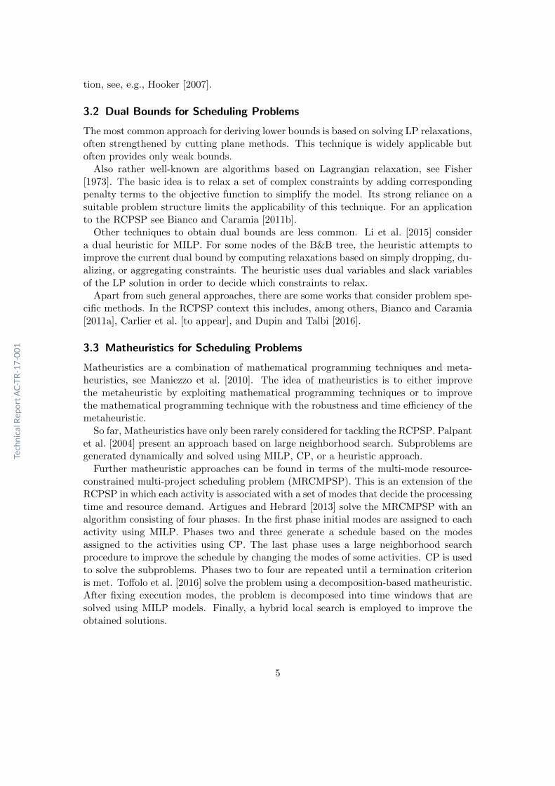
3.2 Dual Bounds for Scheduling Problems

The most common approach for deriving lower bounds is based on solving LP relaxations,often strengthened by cutting plane methods. This technique is widely applicable butoften provides only weak bounds.

Also rather well-known are algorithms based on Lagrangian relaxation, see Fisher[1973]. The basic idea is to relax a set of complex constraints by adding correspondingpenalty terms to the objective function to simplify the model. Its strong reliance on asuitable problem structure limits the applicability of this technique. For an applicationto the RCPSP see Bianco and Caramia [2011b].

Other techniques to obtain dual bounds are less common. Li et al. [2015] considera dual heuristic for MILP. For some nodes of the B&B tree, the heuristic attempts toimprove the current dual bound by computing relaxations based on simply dropping, du-alizing, or aggregating constraints. The heuristic uses dual variables and slack variablesof the LP solution in order to decide which constraints to relax.

Apart from such general approaches, there are some works that consider problem spe-cific methods. In the RCPSP context this includes, among others, Bianco and Caramia[2011a], Carlier et al. [to appear], and Dupin and Talbi [2016].

3.3 Matheuristics for Scheduling Problems

Matheuristics are a combination of mathematical programming techniques and meta-heuristics, see Maniezzo et al. [2010]. The idea of matheuristics is to either improvethe metaheuristic by exploiting mathematical programming techniques or to improvethe mathematical programming technique with the robustness and time efficiency of themetaheuristic.

So far, Matheuristics have only been rarely considered for tackling the RCPSP. Palpantet al. [2004] present an approach based on large neighborhood search. Subproblems aregenerated dynamically and solved using MILP, CP, or a heuristic approach.

Further matheuristic approaches can be found in terms of the multi-mode resource-constrained multi-project scheduling problem (MRCMPSP). This is an extension of theRCPSP in which each activity is associated with a set of modes that decide the processingtime and resource demand. Artigues and Hebrard [2013] solve the MRCMPSP with analgorithm consisting of four phases. In the first phase initial modes are assigned to eachactivity using MILP. Phases two and three generate a schedule based on the modesassigned to the activities using CP. The last phase uses a large neighborhood searchprocedure to improve the schedule by changing the modes of some activities. CP is usedto solve the subproblems. Phases two to four are repeated until a termination criterionis met. Toffolo et al. [2016] solve the problem using a decomposition-based matheuristic.After fixing execution modes, the problem is decomposed into time windows that aresolved using MILP models. Finally, a hybrid local search is employed to improve theobtained solutions.

5


Moreover, there are resemblances to Benders and Lagrangian-based techniques, e.g.,Maniezzo and Mingozzi [1999], Mohring et al. [2003].

3.4 Time Aggregation Models

Note that the contributions mentioned in this section stay in contrast to a more commonapproach in which the time-discretization is coarsened in order to possibly obtain feasiblebut also less precise solutions, which are in general not optimal for the original problem.The approaches discussed here are characterized by iteratively refining a relaxation ofthe original problem until a provably optimal solution is found.

Boland et al. [2017] consider such an approach for the countinuous time service net-work design problem (CTSNDP). The authors solve the problem using a time-expandednetwork. Initially, only a partially time-expanded network is considered to avoid thesubstantial size of the complete network. The MILP model associated with the reducednetwork constitutes a relaxation to the original problem. If the optimal solution to thisrelaxation turns out to be feasible w.r.t. the original problem, the algorithm terminates.Otherwise, the partially time-expanded network is extended based on the current solu-tion to obtain a more refined model. Iteratively applying this approach converges to anoptimal solution due to the finite size of the full time-expanded network.

A different type of relaxation is to partition the given time horizon into subsets.Such approaches are presented by Bigras et al. [2008], Baptiste and Sadykov [2009],and Boland et al. [2016] for single machine scheduling problems. Iterative approachesbased on these techniques have been primarily considered in terms of routing problems.Wang and Regan [2002] and Wang and Regan [2009] consider such an algorithm for thetraveling salesman problem with time windows (TSPTW). First, the time windows ofeach node are partitioned into subsets. Then, for a given time window partitioning alower bound and an upper bound are calculated, using an underconstrained MILP modeland an overconstrained one. If the gap between lower and upper bound is not sufficientlysmall, the scheduling horizon gets further refined and the problem is solved anew.

Another algorithm of this type has been considered by Macedo et al. [2011] for solvingthe vehicle routing problem with time windows and multiple routes (MVRPTW). Theysolve a relaxation which is modeled as a network flow s.t. nodes of the graph correspondto time instants. The idea of the initial relaxation is to aggregate several time instantsinto each node. If the solution to the relaxation turns out to be infeasible w.r.t. theoriginal problem, the current time discretization is locally refined by considering furthertime instants individually, i.e., by disaggregating nodes.

Dash et al. [2012] combine the ideas of Wang and Regan [2002] and Bigras et al. [2008]in order to solve the TSPTW. The time windows of the nodes are partitioned into bucketsusing an iterative refinement heuristic. Refinement decisions are based on the solutionto the current LP relaxation. Afterwards, the resulting formulation is turned into anexact approach by adding valid inequalities and solved using branch-and-cut (B&C). Ineach node of the B&B tree a primal heuristic is applied using the reduced costs of thevariables of the current LP solution.

Recently, Clautiaux et al. [2017] introduced an approach that is more generally ap-

6


plicable to problems that can be modeled as minimum-cost circulation problems withlinking bound constraints. The proposed algorithm projects the original problem onto anaggregated approximate one. This aggregated model is iteratively refined until a prov-ably optimal solution is found. Experiments have been conducted on a routing problemand a cutting-stock problem.

4 Reference MILP Models

In this section, we present two MILP models for SI-PTPSP following classical ap-proaches: a discrete-event formulation (DEF) and a time-indexed formulation (TIF).Both serve as reference formulations to which we will compare our iterative time-bucketrefinement algorithm (ITBRA).

4.1 Discrete Event Formulation

The discrete-event formulation (DEF) is based on the idea of considering certain eventsthat need to be ordered and for which respective times need to be found, see also modelSEE in Artigues et al. [2013]. Resource constraints then only have to be checked at thetimes associated with these events.

In regard to our problem, the considered events are the start and the end of each activ-ity (activity events), and times at which the availability of a resource changes (resourceevents). To simplify the model, we transform all resource events into activity events byintroducing a new artificial activity for each period during which a resource r ∈ R isunavailable. To this end, we create a new activity for each maximal interval in T \Wr

requiring the resource where the processing time is the length of the interval, and the re-lease time and the deadline are the start and the end of the interval, respectively. Then,we define a new set of activities A′ being the union of A and the artificial activities;let α′ = |A′|. Consequently, we denote by K = {1, . . . , 2α′} the set of chronologicallyordered events.

To state the model we use binary variables xa,k that are one if event k ∈ K is the startof activity a ∈ A and zero otherwise. Similarly, binary variables ya,k indicate whetherevent k is the end of activity a. Variables Ek represent the time assigned to each eventk. The starting times of the activities a ∈ A′ are modeled using variables Sa. Finally,binary variables Dr,k are one if resource r ∈ R is used by any activity immediately afterevent k and zero otherwise, and variable MS denotes the makespan.

min MS (1)

Sa + pa ≤ MS ∀a ∈ A (2)

Sa′ − Sa ≥ pa + Lmina,a′ ∀(a, a′) ∈ P (3)

Sa′ − Sa ≤ pa + Lmaxa,a′ ∀(a, a′) ∈ P (4)

∑

k∈Kxa,k = 1 ∀a ∈ A′ (5)

7


∑

k∈Kya,k = 1 ∀a ∈ A′ (6)

∑

a∈A′(xa,k + ya,k) = 1 ∀k ∈ K (7)

Ek−1 ≤ Ek ∀k ∈ K \ {1} (8)

Ek −M (9)a,k(1− xa,k) ≤ Sa ∀k ∈ K, a ∈ A′ (9)

Ek +M(10)a,k (1− xa,k) ≥ Sa ∀k ∈ K, a ∈ A′ (10)

Ek −M (11)a,k (1− ya,k) ≤ Sa + pa ∀k ∈ K, a ∈ A′ (11)

Ek +M(12)a,k (1− ya,k) ≥ Sa + pa ∀k ∈ K, a ∈ A′ (12)

Dr,0 =∑

a∈A′:r∈Qa

xa,0 ∀r ∈ R (13)

Dr,k = Dr,k−1 +∑

a∈A′:r∈Qa

xa,k −∑

a∈A′:r∈Qa

ya,k ∀k ∈ K \ {1}, r ∈ R (14)

Dr,k ≤ 1 ∀k ∈ K, r ∈ R (15)

tra ≤ Sa ≤ tda − pa a ∈ A′ (16)

MS , Ek, Dr,k ≥ 0∀k ∈ K, a ∈ A′,

r ∈ R (17)

xa,k, ya,k ∈ {0, 1} ∀k ∈ K, a ∈ A′ (18)

Inequalities (2) are used for determining the makespan. Precedence relations are enforcedby Inequalities (3) and (4). According to Equalities (5) and (6) each activity startsand ends at precisely one event. Equalities (7) ensure that each event is assigned toeither exactly one starting time or exactly one ending time of an activity. Events areordered chronologically by Inequalities (8). Starting times of activities are linked to thecorresponding start events by Inequalities (9) and (10). Similarly, Inequalities (11) and(12) link the event at which an activity a ends to the time at which the activity ends.Big-M constants used in these inequalities will be explained below. Equalities (13) and(14) compute the total demand of a resource of all activities running during an event.Finally, Inequalities (15) ensure that all resource demands are met at all events.

Choosing the smallest possible Big-M constants for Inequalities (9)–(12) in DEF isimportant for making its LP relaxation as tight as possible. An easy way to set them is

M(9)a,k = Tmax−tra, M (10)

a,k = tda−pa−Tmin, M(11)a,k = Tmax−tra−pa, and M

(12)a,k = tda−Tmin.

However, by computing sets of activities that must precede or succeed a certain eventin any feasible schedule, respectively, it is possible to fix some constants to zero. Fordetails, we refer to Jatschka [2017].

The formulation has O(|A′|2) variables and O(|R| · |A′|2) constraints. Thus, DEF is acompact model, but its LP relaxation typically yields rather weak LP bounds, primarilydue to the inequalities involving the Big-M constants.

8


4.2 Time-indexed Formulation

In a classical MILP way, we can model SI-PTPSP by the following time-indexed formu-lation (TIF) using binary variables xa,t for indicating whether an activity a ∈ A startsat time t ∈ Ta.

min MS (19)∑

t∈Taxa,t = 1 ∀a ∈ A (20)

∑

t∈Tat · xa,t + pa ≤ MS ∀a ∈ A (21)

∑

a∈A:r∈Qa

∑

t′∈Ta:t∈Ya(t′)

xa,t′ ≤ 1 ∀r ∈ R, t ∈Wr (22)

∑

t∈Ta′txa′,t −

∑

t∈Tatxa,t ≥ pa + Lmin

a,a′ ∀(a, a′) ∈ P (23)

∑

t∈Ta′txa′,t −

∑

t∈Tatxa,t ≤ pa + Lmax

a,a′ ∀(a, a′) ∈ P (24)

xa,t ∈ {0, 1} ∀a ∈ A, t ∈ Ta (25)

MS ≥ 0 (26)

Equations (20) ensure that exactly one starting time is chosen for each activity. Inequal-ities (21) are used to determine the makespan MS . Resource restrictions are enforcedby Inequalities (22). Last but not least, Constraints (23) and (24) guarantee that theprecedence relations with their minimum and maximum time lags are respected.

The model has O(|A|·|T |) variables and O(|T |·(|A|+|R|+|P |)) constraints. Typically,the LP relaxation of TIF yields substantially tighter dual bounds than the LP relaxationof DEF but its size and solvability strongly depend on the used time discretization, i.e.,|T |.

5 Time-Bucket Relaxation

As the number of variables and constraints of TIF becomes fairly large when consider-ing a fine-grained time discretization, directly solving the model may not be a viableapproach in practice. We therefore consider a relaxation of it, in which we combinesubsequent time slots into so-called time-buckets. This model, which we call time-bucketrelaxation (TBR), yields a dual bound to the optimal value of the original problem butin general not a valid solution. Based on TBR we will build our iterative refinementapproach in Section 6.

Let B = {B1, . . . , Bβ} be a partitioning of T into subsequent time-buckets. Notethat the individual buckets do not need to have the same size. We denote by I(B) ={1, . . . , β} the index set of B. For all b ∈ I(B) we define the set of consecutive timeslots Bb = {Bstart

b , . . . , Bendb } contained in the bucket. Since B is a chronologically

9


B1 B2 B3 B4 B5 B6 · · · Bβ

Tmin Tmax

Figure 1: Bucket partitioning of T .

ordered partitioning of T , we have Bstart1 = Tmin, Bend

β = Tmax, and Bendb + 1 = Bstart

b+1 ,

∀b ∈ I(B)\{β}. For an illustration see Fig. 1. Additionally, letWBr (b) = |Bb∩Wr| denote

the aggregated amount of resource r ∈ R available over the whole bucket b ∈ I(B).Considering a bucket partitioning we now derive for each activity a ∈ A all subsets

of buckets in which the activity can be completely performed s.t. it executes at leastpartially in every bucket. We call these subsets bucket sequences of activity a and denotethem by Ca = {Ca,1, . . . , Ca,γa} ⊆ 2I(B). Let functions bfirst(a, c) and blast(a, c) for a ∈A and c = 1, . . . , γa provide the index of the first and the last bucket of bucket sequenceCa,c, respectively. The bucket sequences in Ca are assumed to be ordered accordingto increasing starting time, or, more precisely, lexicographically ordered according to(bfirst(a, c),blast(a, c)). We can determine all bucket sequences for an activity in timeO(|B| log |B|), for details see Section 7.2. Analogous to set Ta we do not consider bucketsequences that involve only infeasible starting times.

For each bucket sequence let Smina,c ∈ T be the earliest time slot at which activity a can

feasibly start when it is assigned to bucket sequence Ca,c ∈ Ca. Similarly, let Smaxa,c ∈ T

be the latest possible starting point. Moreover, values zmina,b,c and zmax

a,b,c provide boundson the number of utilized time slots within bucket b ∈ Ca,c when activity a uses bucket-sequence Ca,c ∈ Ca. Note that for inner buckets b with bfirst(a, c) < b < blast(a, c) wealways have zmin

a,b,c = zmaxa,b,c = |Bb|. Fig. 2 shows a set of bucket sequences for a given

activity. Observe that for bucket sequence Ca,2 we need to shift the execution windows.t. the activity executes at least for one time slot in bucket B3, i.e., we require zmin

a,3,2 > 0to avoid an overlap with bucket sequence Ca,1.

Our relaxation of TIF uses binary variables ya,c indicating whether activity a ∈ A isperformed in bucket sequence Ca,c for c ∈ {1, . . . , γa}. Model TBR is stated as follows:

min MS (27)γa∑

c=1

ya,c = 1 ∀a ∈ A (28)

γa∑

c=1

Smina,c · ya,c + pa ≤ MS ∀a ∈ A (29)

∑

a∈A:r∈Qa

∑

Ca,c∈Ca:b∈Ca,c

zmina,b,c · ya,c ≤WB

r (b) ∀r ∈ R, b ∈ I(B) (30)

10


B1 B2 B3 B4 B5 Ca,1 = {B1, B2}

tra tdapa

zmina,2,1zmax

a,1,1

pa

zmina,1,1

zmaxa,2,1

B1 B2 B3 B4 B5 Ca,2 = {B1, B2, B3}

pa

zmina,3,2zmax

a,1,2

pa

zmina,1,2

zmaxa,3,2

B1 B2 B3 B4 B5 Ca,3 = {B2, B3, B4}

pa

zmina,4,3zmax

a,2,3

pa

zmina,2,3 zmin

a,4,3

B1 B2 B3 B4 B5 Ca,4 = {B3, B4, B5}

pa

zmina,5,4zmax

a,3,4

pa

zmina,3,4

zmaxa,5,4

B1 B2 B3 B4 B5Ca,5 = {B4, B5}

pa

zmina,5,5zmax

a,4,5

pa

zmina,4,5

zmaxa,5,5

Figure 2: Bucket sequences Ca of an activity a with processing time pa. Descriptions ofinner buckets of a sequence are omitted since zmin

a,b,c = zmaxa,b,c = |Bb| holds for

them.

11


γa′∑

c′=1

Smaxa′,c′ · ya′,c′ −

γa∑

c=1

Smina,c · ya,c ≥ pa + Lmin

a,a′ ∀(a, a′) ∈ P (31)

γa′∑

c′=1

Smina′,c′ · ya′,c′ −

γa∑

c=1

Smaxa,c · ya,c ≤ pa + Lmax

a,a′ ∀(a, a′) ∈ P (32)

ya,c ∈ {0, 1} ∀a ∈ A,c = 1, . . . , γa

(33)

MS ≥ 0 (34)

Equations (28) ensure that exactly one bucket sequence is chosen for each activity. Themakespan MS is determined using Inequalities (29). Constraints (30) consider the re-source availabilities individually for each bucket in an accumulated fashion. Determinedresource consumptions of activities are precise for all used inner buckets of a sequencebut might underestimate the actually required amount in the first and last bucket. Fi-nally, Inequalities (31) and (32) realize the precedence constraints with their minimumand maximum time lags, respectively. These restrictions also constitute a relaxation ofthe corresponding ones in TIF since the precise starting times within the buckets arenot known (unless dealing with buckets of unit size).

The model has O(|A| · |B|) variables and O(|A|+ |R| · |B|+ |P |) constraints, and thusits size does not depend on |T |.

5.1 Comparison of TIF and TBR

First, let us consider the case of TBR in which all buckets have unit size, i.e., B ={{Tmin}, {Tmin + 1}, . . . , {Tmax}}. Let us denote this special case by TBR1. This leadsto several simplifications. All buckets b belonging to some sequence Ca,c are fully used,i.e., zmin

a,b,c = zmaxa,b,c = |Bb| = 1. Moreover, minimum and maximum starting times are equal

and equivalent to the first time slot of the initial bucket of the sequence: Smina,c = Smax

a,c =

Bstartbfirst(a,c). Essentially, this means that Ta = {Smin

a,c | Ca,c ∈ Ca} = {Smaxa,c | Ca,c ∈ Ca}

and |Ta| = |Ca| for all a ∈ A. Furthermore, since buckets correspond to original timeslots in this scenario, resource availabilities become binary for each bucket.

For TIF and TBR1 we consider function ϕa : {1, . . . γa} → Ta for each activity a ∈ Awith ϕa(c) := Smin

a,c .

Proposition 1. Function ϕ is bijective.

Proof. Each bucket sequence w.r.t. TBR1 corresponds to a specific starting time. Foreach activity Ca considers all feasible bucket sequences and Ta all feasible starting times.Thus, there exists a unique mapping between these sets.

Proposition 2. The polyhedra of TBR1 and TIF are isomorphic.

Proof. We establish an isomorphism between the variables of the models using functionϕa and its inverse: xa,t = ya,ϕ−1

a (t) and ya,c = xa,ϕa(c). Moreover, we can use these

12


functions to immediately transform (20) into (28), (21) into (29), (23) into (31), and (24)into (32) and vice versa. To provide the isomorphism between (22) and (30) we need afew further things. First, recall that all zmin

a,b,c constants are equal to 1. Second, using

t↔ {t} as isomorphism between T and the set of unit buckets we obtain WBr (b) = 1 if the

corresponding time point t ∈Wr and WBr (b) = 0 otherwise. Finally, the correspondence

between time points and unit buckets guarantees that Ya(t) and Ca,c are isomorphic forϕ−1a (t) = c. Putting things together also the resource constraints can be transformed

into one another.

Corollary 1. The LP relaxations of TBR1 and TIF are equally strong.

Definition 1. Let TBRB and TBRB′ be two TBR-models with bucket partitionings Band B′, respectively. TBRB′ is called a refined model of TBRB iff ∀b′ ∈ I(B′) ∃b ∈I(B) (B′b′ ⊆ Bb).

In the following we show that TBRB is a relaxation of TBRB′ and thus of TIF.

Definition 2. Let TBRB be a TBR-model and let TBRB′ be a refined model of TBRB.Then, σ : C ′a → Ca defines a (surjective) mapping from bucket sequences C ′a w.r.t. TBRB′

to bucket sequences Ca w.r.t. TBRB satisfying for all C ′a,c′ ∈ C ′a:

⋃

b′∈C′a,c′

b′ ⊆⋃

b∈σ(C′a,c′ )

b ∧ ∀Ca,c ∈ Ca

⋃

b′∈C′a,c′

b′ *⋃

b∈Ca,c

b ∨ σ(C ′a,c′) ⊆ Ca,c

.

This means σ provides the inclusion minimal bucket sequence from TBRB that con-tains at least the time slots that the bucket sequence from TBRB′ contains.

Lemma 1. Function σ can be implemented by:

σ(C ′a,c′) = Ca,c s.t. Ca,c ∈ Ca ∧ Smina,c′ ∈ bfirst(a, c) ∧ (Smin

a,c′ + pa) ∈ blast(a, c)

Proof. Feasibility of C ′a,c′ together with the fact that buckets in TBRB′ are subsets

of those in TBRB implies that there exists a sequence Ca,c ∈ Ca satisfying Smina,c′ ∈

bfirst(a, c) and (Smina,c′ + pa) ∈ blast(a, c). The buckets of sequence C ′a,c′ are contained

in those of sequence Ca,c, i.e.,⋃b′∈C′

a,c′b′ ⊆ ⋃b∈Ca,c

b. Moreover, Ca,c is uniquely deter-

mined since by definition two different bucket sequences cannot have the same first andlast buckets. Therefore, every other sequence covering the buckets from C ′a,c′ must bestrictly larger than Ca,c.

Theorem 1. Let TBRB be a TBR-model and let TBRB′ be a refined model of TBRB.Then, TBRB is a relaxation of TBRB′.

Proof. Using function σ according to Lemma 1, we create a solution y to TBRB froman optimal solution y∗ to TBRB′ as follows:

ya,c =∑

C′a,c′∈C′a:σ(C′

a,c′ )=Ca,c

y∗a,c′ ∀a ∈ A, c ∈ {1, . . . , γa}

13


We first show that y is a feasible solution for TBRB. Constraints (28) are satisfied sincey∗a,c′ is feasible and σ is surjective. As bfirst(a, c′) ⊆ bfirst(a, c) for all Ca,c = σ(C ′a,c′)it holds that Smin

a,c ≤ Smina,c′ and Smax

a,c′ ≤ Smaxa,c . Hence, Constraints (29), (31), and (32)

must hold. If Inequalities (30) are satisfied for y∗, then the resource constraints are alsosatisfied for y since the refined resource allocation entails the coarser one. Therefore, yis a feasible solution to TBRB.

Since Smina,c ≤ Smin

a,c′ , the objective can only decline due to the transformation. Thus,the optimal solution value to TBRB can be at most as large as the value of the optimalsolution to TBRB′ . Thus, TBRB is a relaxation of TBRB′ .

Corollary 2. TBR is a relaxation of TIF.

5.2 Strengthening TBR by Valid Inequalities

In the following we introduce two types of valid inequalities to compensate for the loss ofaccuracy in TBR due to the bucket aggregation. Note that these inequalities strengthenthe relaxation in general but might become redundant for more fine-grained bucketpartitionings.

5.2.1 Clique Inequalities

Observe that two activities, represented by non-unit bucket sequences, cannot feasiblystart in the same bucket if both require a certain resource. The same holds for two ormore bucket sequences with these properties ending in the same bucket. This can beused to derive sets of incompatible bucket sequences that give rise to clique inequalities,see Demassey et al. [2005], Hardin et al. [2008].

To formulate respective constraints we determine for each b ∈ I(B) sets Sb = {(a, c) |a ∈ A, c ∈ Ca, z

mina,b,c < |Bb|, |Ca,c| > 1, bfirst(a, c) = b} and Fb = {(a, c) | a ∈ A, c ∈

Ca, zmina,b,c < |Bb|, |Ca,c| > 1,blast(a, c) = b} of non-unit bucket sequences starting and

ending in bucket Bb, respectively. From each of these sets we derive a graph havingthe respective set as nodes and an edge between two nodes if the activities of the corre-sponding bucket sequences share a resource. Let CSb and CFb be the sets of all maximalcliques with a minimum size of two within these graphs. This leads to the followinginequalities:

∑

(a,c)∈κya,c ≤ 1, ∀b ∈ I(B),∀κ ∈ CSb (35)

∑

(a,c)∈κya,c ≤ 1, ∀b ∈ I(B), ∀κ ∈ CFb (36)

Some of these constraints might be redundant if the sum of zmina,b,c of the smallest two

sequences is already large enough to prohibit them from being in the same bucket bymeans of Inequalities (30). The most trivial form of this case is excluded in the abovesets by the condition zmin

a,b,c < |Bb|.

14


The considered cliques can be computed using the algorithm by Bron and Kerbosch[1973]. Cazals and Karande [2008] show that this algorithm is worst-case optimal, i.e.,it runs in O(3

n3 ) which is the largest possible number of maximal cliques in a graph on

n nodes. Although problematic in general, this might still be reasonable considering therather small expected size of the conflict graphs.

Nevertheless, in our implementation we decided to avoid clique computations and re-sort to a simpler variant. We do so by considering a separate graph per resource obtaininga set of not necessarily maximal cliques. This leads to conceptually weaker inequalitiesbut requires almost no computational overhead. More specifically, we consider subsetsSb,r = Sb ∩ {(a, c) | a ∈ A, c ∈ Ca, r ∈ Qa} of Sb and subsets Fb,r = Fb ∩ {(a, c) | a ∈A, c ∈ Ca, r ∈ Qa} of Fb, respectively, for b ∈ I(B) and r ∈ R s.t. within these subsetsall activities require a common resource. Using these sets we formulate the followingconstraints:

∑

(a,c)∈Sb,rya,c ≤ 1, ∀b ∈ I(B),∀r ∈ R : |Sb,r| ≥ 2 (37)

∑

(a,c)∈Fb,r

ya,c ≤ 1, ∀b ∈ I(B),∀r ∈ R : |Fb,r| ≥ 2 (38)

If mutual overlap of the resources required by the activities is rare, the simpler in-equalities are often almost as powerful as the full clique inequalities.

5.2.2 Path Inequalities

The idea of this kind of inequalities is to extend the precedence constraints (31) and (32)and the makespan constraints (34) to be valid for paths in the precedence graph insteadof only for adjacent activities.

We consider the acyclic directed precedence graph G = (A,P ). Let πa0,am = (a0, a1,. . . , am) be a directed path from activity a0 to activity am in G. Moreover, let minimumand maximum path lengths dLmin(πa0,am) =

∑m−1i=0 pai + Lmin

ai,ai+1and dLmax(πa0,am) =∑m−1

i=0 pai + Lmaxai,ai+1

be the minimum and maximum makespan of the activities withinthe path, respectively. Let Πa,a′ denote the set of all distinct paths from node a to nodea′. Since G is acyclic, Πa,a′ is finite (but in general exponential in the number of edges)for all pairs of nodes (a, a′) ∈ A×A : a 6= a′. Let Π =

⋃a,a′∈A:a6=a Πa,a′ denote the union

of all these paths between any two different nodes.Let S be a feasible solution to SI-PTPSP. Then, for each path πa,a′ in G it must hold

that Sa + dLmin(πa,a′) ≤ Sa′ and Sa + dLmax(πa,a′) ≥ Sa′ . Hence, adding the followinginequalities for all πa,a′ ∈ Π to TBR yields a strengthened relaxation of TIF:

γa∑

c=1

Smina,c · ya,c + dLmin(πa,a′) ≤

γa′−1∑

c′=0

Smaxa′,c′ · ya′,c′ (39)

γa∑

c=1

Smaxa,c · ya,c + dLmax(πa,a′) ≥

γa′−1∑

c′=0

Smina′,c′ · ya′,c′ (40)

15


γa∑

c=1

Smina,c · ya,c + dLmin(πa,a′) + pa′ ≤ MS (41)

Due to the exponential number of these inequalities we only consider a reasonablesubset of them in our implementation, for details see Section 7.3.

6 Iterative Time-Bucket Refinement Algorithm

For the original SI-PTPSP, TBR on its own is a method yielding a lower bound butno concrete feasible solution. The basic idea of the iterative time-bucket refinementalgorithm (ITBRA) is to solve TBR repeatedly, refining the bucket partitioning in eachiteration, until a proven optimal solution can be derived via primal heuristics or someother termination criterion is met. We will show that, given enough time, this algorithmconverges to an optimal SI-PTPSP solution.

More specifically, we start by solving TBR with an initial bucket partitioning. Then,we try to heuristically derive a feasible SI-PTPSP solution that matches the objectivevalue of TBR with a so-called gap closing heuristic (GCH). This heuristic fixes concretetimes for activities in accordance with the TBR solution and guarantees to never violateresource or precedence constraints. If all activities can be scheduled in this way, we havefound and optimal solution and the algorithm terminates. Otherwise, some activitiesremain unscheduled and we apply a follow-up heuristic to augment and repair the partialsolution, possibly obtaining a feasible approximate solution and a primal bound. Hereit can again be the case that we are able to close the optimality gap. If no provablyoptimal solution has been found thus far, we refine the bucket partitioning by splittingselected buckets and solve TBR again. For selecting the buckets to be refined and doingthe splitting, we exploit information obtained from the TBR solution and the appliedprimal heuristics. This process is iterated until specified termination criteria are metor an optimal solution is found. The whole procedure is shown in Algorithm 1. Theindividual components of this approach will be explained in detail in the next sections.

6.1 Initial Bucket Partitioning

We create the initial bucket partitioning B in such a way that buckets start/end at anytime when a resource availability interval starts or ends and at any release time anddeadline of the activities. For details see Algorithm 2.

6.2 Primal Heuristics

We consider heuristics that attempt to derive feasible SI-PTPSP solutions and corre-sponding primal bounds based on TBR solutions. If ITBRA is terminated early, the bestsolution found in this way is returned. Note, however, that depending on the instanceproperties, these heuristics might also fail and then yield no feasible solution.

16


Algorithm 1: Iterative time-bucket refinement algorithm (ITBRA)

Input: SI-PTPSP instanceOutput: solution to SI-PTPSP and lower bound

1: compute initial bucket partitioning;2: compute initial primal solution;3: do4: solve TBR for the current bucket partitioning;5: apply gap closing heuristic (GCH): try to find an SI-PTPSP solution in

accordance with the TBR solution;6: if unscheduled activities remain then7: apply follow-up heuristic to find feasible SI-PTPSP solution8: end if9: if gap closed then

10: return optimal solution11: end if12: derive refined bucket partitioning for the next iteration;

13: while termination criteria not met ;14: return best heuristic solution and lower bound from TBR

6.2.1 Gap Closing Heuristic (GCH)

This is the first heuristic applied during an iteration of ITBRA. It attempts to constructan optimal solution according to TBR’s result to close the optimality gap. Thus, itmay only fully succeed when the relaxation’s objective value does not underestimate theoptimal SI-PTPSP solution value. If the gap cannot be closed, GCH provides only apartial solution and no primal bound. Information on the unscheduled activities thenforms an important basis for the subsequent bucket refinement.

Let (y∗,MS ∗) be the current optimal TBR solution. Initially, GCH receives for eachactivity a ∈ A the interval STBR

a = {STBR,mina , . . . , STBR,max

a } of potential starting times,

Algorithm 2: Computing an initial bucket partitioning

Output: the initial bucket partitioning1: B ← ∅; // bucket partitioning

2: T ← {Tmin} ∪ {Tmax + 1}; // bucket starting times

3: T ← T ∪ {W startr,w ,W end

r,w + 1 | r ∈ R, w = 1, . . . , ωr};4: T ← T ∪ {tra, tda | a ∈ A};5: sort T ;6: for i← 1 to |T | − 1 do7: B ← B ∪ {{T [i], . . . , T [i+ 1]− 1}}; // add bucket

8: end for9: return B;

17


where STBR,mina =

∑γa−1c=0 Smin

a,c · y∗a,c and STBR,maxa =

∑γa−1c=0 Smax

a,c · y∗a,c. These intervals

can in general be further reduced by removing for each a ∈ A all time slots t ∈ STBRa

violating at least one of the following conditions in relation to the precedence constraintsand the calculation of the makespan:

∃t′ ∈ STBRa′ (t+ pa + Lmin

a,a′ ≤ t′ ≤ t+ pa + Lmaxa,a′ ) ∀(a, a′) ∈ P (42)

∃t′ ∈ STBRa′ (t′ + pa′ + Lmin

a′,a ≤ t ≤ t′ + pa′ + Lmaxa′,a ) ∀(a′, a) ∈ P (43)

t+ pa ≤ MS ∗ (44)

We prune the set of intervals of potential activity starting times for all activitiesSTBR = {STBR

a | a ∈ A} so that arc consistency is achieved w.r.t. Conditions (42)–(44).This is done by constraint propagation with a method like the well-known AC3 algorithm,see Mackworth [1977]. Note that this constraint propagation may yield empty intervalsfor some activities, indicating that there remains no feasible starting time assignmentrespecting all constraints. In this case GCH will give up on this activity and continueswith the remaining ones deviating from the usual arc consistency concept to allow furtheractivities to be scheduled.

The pseudocode of GCH is shown in Algorithm 3. After the initial pruning of startingtime intervals, GCH constructs the (partial) schedule S by iteratively scheduling theactivities respecting all constraints. If this is not possible for some activities, they remainunscheduled. Using a greedy strategy, the activities are considered in non-decreasingorder of STBR,max

a +pa, i.e., according to their earliest possible finishing times. Activitiesare always scheduled at the earliest feasible time from STBR

a . Note that any explicitenumeration of time slots from an interval can be efficiently avoided by using basicinterval arithmetic. Whenever an activity starting time is set, constraint propagation isrepeated to ensure arc consistency according to Conditions (42)–(44).

If GCH fails to close the gap, we attempt to compute a feasible solution instead thatmight have a larger objective value than the current TBR bound.

6.2.2 Activity Block Construction Heuristic (ABCH)

This algorithm is based on the idea of first constructing so-called activity blocks, whichcorrespond to the weakly connected components of the precedence graph. All the activi-ties belonging to one such weakly connected component are statically linked consideringthe precedence constraints and minimum time lags between them. ABCH then greedilyschedules the activity blocks that have not been scheduled completely by GCH insteadof the individual activities. The activity blocks are considered in order of their releasetimes and are scheduled at the first time slot where no resource constraint is violatedw.r.t. the activity block’s individual activities and resource requirements. Details areprovided in Algorithm 4.

6.2.3 Greedy Randomized Adaptive Search Procedure (GRASP)

GRASP is a prominent metaheuristic that applies a randomized variant of a constructionheuristic followed by a local search component independently many times, where the

18


Algorithm 3: Gap closing heuristic (GCH)

Input: intervals of potential starting times STBR = {STBRa | a ∈ A} with

STBRa = {STBR,min

a , . . . , STBR,maxa }

Output: (partial) schedule S and all activities that cannot be scheduled w.r.t.STBR grouped by violation type

1: AP ← ∅; // activities with violated precedence constraints

2: AR ← ∅; // activities with violated resource constraints

3: AU ← A; // unscheduled activities

4: W ′r ←Wr; // resource availabilities

5: prune potential starting time intervals STBR;6: while AU 6= ∅ do7: select and remove an activity a ∈ AU with minimal STBR,max

a + pa;8: if STBR

a = ∅ then // precedence constraints violated

9: AP ← AP ∪ {a};10: continue;

11: end if

12: STBRa ← {t ∈ STBR

a | {t, . . . , t+ pa − 1} ⊆W ′r, ∀r ∈ Qa};13: if STBR

a = ∅ then // resource constraints violated

14: AR ← AR ∪ {a};15: continue;

16: end if

17: Sa ← min STBRa ;

18: STBRa ← {Sa};

19: W ′r ←W ′r \ {t, . . . , t+ pa − 1}, ∀r ∈ Qa;20: prune potential starting time intervals STBR;

21: end while22: return S,AP , AR;

best found solution is kept as the result, see Resende and Ribeiro [2010]. We considerGRASP here as an advanced alternative to ABCH within ITBRA. The approach providesa reasonable balance between being still relatively simple but providing considerablybetter results than ABCH. There are clearly other options but our aim here is to keepstandard metaheuristic aspects simple in order to put more emphasis on TBR’s andITBRA’s fundamentals.

Both, GCH and ABCH can be randomized. We do so by allowing the order in whichthe activities or activity blocks are considered to deviate from the strict greedy criterion.In particular, we choose uniformly at random from the kgrand

GCH (kgrandABCH) candidates with

the highest priority. Parameters kgrandGCH and kgrand

ABCH control the strength of the random-ization. Note that the success of ABCH and hence also of the GRASP strongly dependson the partial solution provided by GCH. Therefore, we primarily choose to randomizeGCH. We also try to compute a primal solution at the very beginning before solving

19


Algorithm 4: Activity block construction heuristic (ABCH)

Input: a partial schedule SGCH computed by GCHOutput: a feasible schedule S or no solution if SGCH cannot be completed

1: C ← set of subsets of A corresponding to the weakly connected components ofthe precedence graph which are not completely scheduled in SGCH;

2: AC ← ∅; // the set of activity blocks

3: forall weakly connected components c ∈ C do4: Sc ← ∅ ; // a schedule representing the activity block of c5: forall activities a ∈ c in topological order do6: schedule a in Sc at the earliest possible time w.r.t. the precedence

constraints and resource consumptions of activities in c but ignoring allother activities as well as release times and deadlines, and resourceavailabilities;

7: end8: the release time of the activity block is mina∈c tra;9: AC ← AC ∪ {Sc} ;

10: end11: forall activity blocks Sc ∈ AC ordered according to release time do12: try to schedule the activity block at the earliest feasible time in S s.t. activity

release times and deadlines as well as resource constraints are satisfied;13: if no feasible time found then14: return no solution;15: end if

16: end17: return S;

TBR for the first time. Hence, there is no GCH solution available at this point. In thiscase we randomize ABCH instead.

To get a strong guidance for the bucket refinement process we prefer GCH solutionsthat schedule as many activities as possible. However, these solutions might not necessar-ily correspond to those solutions that work best in conjunction with ABCH. Therefore,we track the best complete solution and the best partial GCH solution separately. Thismeans that our GRASP returns a feasible SI-PTPSP solution as well as a partial GCHsolution (which might be unrelated). Since GRASP combines the functionalities of GCHand ABCH, it effectively replaces Lines 5–8 in Algorithm 1.

We consider a local search component using a classical 2-exchange neighborhood onthe order of the activity blocks scheduled by ABCH. The local search is always performeduntil a local optimum is reached.

As termination criterion for the GRASP a combination of a time limit and a maximalnumber of iterations without improvement is used, details will be given in Section 8.Moreover, in the first iteration of the GRASP the deterministic versions of GCH andABCH are used. This guarantees, especially for short executions, that the final result of

20


B1 B2 B3 B4 B5 B6 · · · Bβ

Tmin Tmaxτ21 τ4

1 τ42

B′1 B′

2 B′3 B′

4 B′5 B′

6 B′7 B′

8 B′9 · · · B′

β

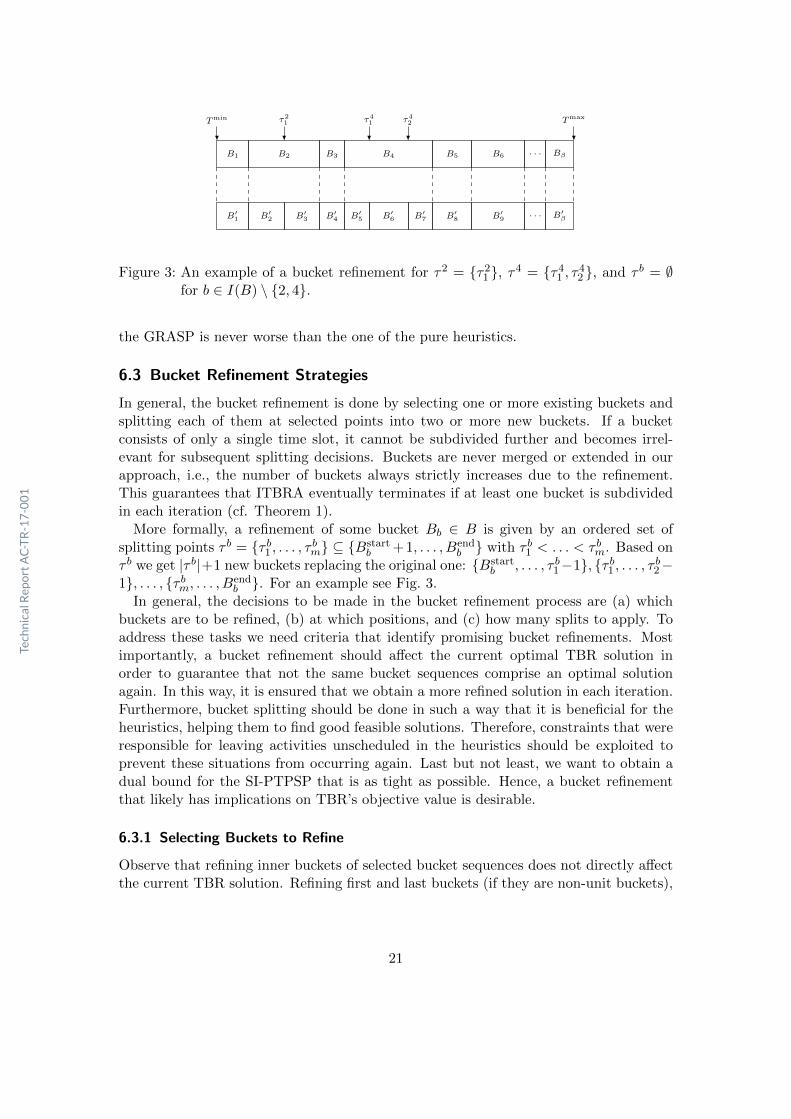
Figure 3: An example of a bucket refinement for τ2 = {τ21 }, τ4 = {τ4

1 , τ42 }, and τ b = ∅

for b ∈ I(B) \ {2, 4}.

the GRASP is never worse than the one of the pure heuristics.

6.3 Bucket Refinement Strategies

In general, the bucket refinement is done by selecting one or more existing buckets andsplitting each of them at selected points into two or more new buckets. If a bucketconsists of only a single time slot, it cannot be subdivided further and becomes irrel-evant for subsequent splitting decisions. Buckets are never merged or extended in ourapproach, i.e., the number of buckets always strictly increases due to the refinement.This guarantees that ITBRA eventually terminates if at least one bucket is subdividedin each iteration (cf. Theorem 1).

More formally, a refinement of some bucket Bb ∈ B is given by an ordered set ofsplitting points τ b = {τ b1 , . . . , τ bm} ⊆ {Bstart

b + 1, . . . , Bendb } with τ b1 < . . . < τ bm. Based on

τ b we get |τ b|+1 new buckets replacing the original one: {Bstartb , . . . , τ b1−1}, {τ b1 , . . . , τ b2−

1}, . . . , {τ bm, . . . , Bendb }. For an example see Fig. 3.

In general, the decisions to be made in the bucket refinement process are (a) whichbuckets are to be refined, (b) at which positions, and (c) how many splits to apply. Toaddress these tasks we need criteria that identify promising bucket refinements. Mostimportantly, a bucket refinement should affect the current optimal TBR solution inorder to guarantee that not the same bucket sequences comprise an optimal solutionagain. In this way, it is ensured that we obtain a more refined solution in each iteration.Furthermore, bucket splitting should be done in such a way that it is beneficial for theheuristics, helping them to find good feasible solutions. Therefore, constraints that wereresponsible for leaving activities unscheduled in the heuristics should be exploited toprevent these situations from occurring again. Last but not least, we want to obtain adual bound for the SI-PTPSP that is as tight as possible. Hence, a bucket refinementthat likely has implications on TBR’s objective value is desirable.

6.3.1 Selecting Buckets to Refine

Observe that refining inner buckets of selected bucket sequences does not directly affectthe current TBR solution. Refining first and last buckets (if they are non-unit buckets),

21


however, ensures that the bucket sequence that contained them does not exist in therefined TBR anymore and therefore cannot be used again. Furthermore, some newlyintroduced buckets might not be part of feasible bucket sequences anymore, resulting ina more restricted scenario. Hence, we want to either split only first or last buckets ofselected sequences or both. If we use just one bucket, we need to resort to the other oneif otherwise no progress can be made. During preliminary tests it turned out that alwaysusing both boundary buckets for refinement is superior. Another question is for whichbucket sequences the bounding buckets shall be refined. In the following we proposedifferent strategies that will be experimentally compared in Section 8.2.2.

All Selected (ASEL) Using this strategy we refine all first and last buckets of allbucket sequences selected in the current optimal TBR solution. This can, however, beinefficient as it may increase the total number of buckets in each iteration substantially.The following strategies will therefore only consider certain subsets.

All In GCH Schedule (AIGS) We refine all first and last buckets of only those bucketsequences whose corresponding activities could be feasibly scheduled by GCH. The idea isto improve accuracy for the scheduled activities in order to reveal sources of infeasibilityw.r.t. the activities that could not be scheduled once TBR is solved the next time.

Violated Due (VDUE) If GCH fails to schedule all activities, it provides a set ofactivities AP that cannot be scheduled due to the precedence constraints and a set ofactivities AR that cannot be scheduled due to the resource constraints. The basic ideais to refine buckets related to activities in the schedule that immediately prevent theactivities in AP and AR from being scheduled. To identify these activities we considerthe partial schedule S generated by GCH.

Let AGCH = A \ (AR ∪ AP ) be the set of feasibly scheduled activities. Refinementsbased on resource infeasibilities are derived from sets NR(a) = {a′ ∈ AGCH | Qa ∩Qa′ 6=∅ ∧ {Sa′ , . . . , Sa′ + pa′ − 1} ∩ {STBR,min

a , . . . , STBR,maxa + pa − 1} 6= ∅} for a ∈ AR. For

each activity a′ ∈ NR(a) we refine the first and last bucket of the bucket sequence Ca′,cin the TBR solution.

The activities potentially responsible for a ∈ AP having no valid starting time are theactivities a′ in AGCH s.t. (a, a′) ∈ P or (a′, a) ∈ P . However, we do not have to considerall activities incident to a for the refinement. Let N−P (a) = {a′ | (a′, a) ∈ P ∧a′ ∈ AGCH}and N+

P (a) = {a′ | (a, a′) ∈ P ∧ a′ ∈ AGCH} for all a ∈ AP . Then, calculate:

NP (a) = arg maxa′∈N−P (a)

{Sa′ + pa′ + Lmina′,a} ∪ arg min

a′∈N−P (a)

{Sa′ + pa′ + Lmaxa′,a } ∪

arg mina′∈N+

P (a)

{Sa′ − Lmaxa,a′ } ∪ arg max

a′∈N+P (a)

{Sa′ − Lmina,a′} (45)

We refine the first and last buckets of all bucket sequences of activities a′ ∈ NP (a)that are selected in the current TBR solution. If no refinement is possible for bucketsequences corresponding to a′ ∈ NR(a) ∪ NP (a), we refine the first and last bucket ofCa,c instead.

22


6.3.2 Identifying Splitting Positions

Once a bucket has been selected for refinement, we have to decide at which position(s) itshall be subdivided. Again, we consider different strategies. The challenge is to identifycandidate positions that usually have a large impact on the subsequent TBR and itssolution while resulting in well-balanced sub-buckets.

Binary (B) Let Ca,c be the bucket sequence causing its first and last buckets to beselected for refinement. We split the selected buckets in such a way that the interval ofpotential starting and finishing times of the respective activity is bisected. In particular,for bfirst(a, c) and blast(a, c), we consider the splitting positions d(Smin

a,c + Smaxa,c )/2e and

d(Smaxa,c + Smin

a,c )/2e + pa, respectively. We have to round up in case of non integralrefinement positions since it is not feasible to refine w.r.t. the bucket start. Althoughthis approach typically leads to well-balanced sub-buckets, it might often have a ratherweak impact on the subsequent TBR solution because the resulting buckets might stillbe too large to reveal certain sources of infeasibility.

Start/End Time (SET) Let a be an activity that could be scheduled by GCH and Ca,cthe corresponding bucket sequence in TBR whose first and last buckets shall be refined.We split bfirst(a, c) at the activity’s starting time Sa and blast(a, c) at Sa+pa, i.e., afteractivity a has ended according to GCH’s schedule. Thus, the specifically chosen timeassignment of GCH gets an individual bucket sequence in the next iteration.

Because this method is defined only for activities that could be scheduled by GCH,it is applicable only in direct combination with AIGS. To overcome this limitation weresort to B if SET is not applicable. The obtained strategy is denoted by SET+B.

6.3.3 Selecting Splitting Positions

The strategies introduced above may yield several splitting positions for a single bucket,especially since the same bucket may be selected multiple times for refinement for dif-ferent activities. In principle, we want to generate as few new buckets as possible whileensuring strong progress w.r.t. the dual bound and narrowing down the activities’ pos-sible starting time intervals. Splitting at all identified positions might therefore not bethe best option. In the following we propose different strategies for selecting for eachselected bucket the splitting positions to be actually used from all positions determinedin the previous step. Let set τ b be this union of identified splitting positions for bucketb.

Union Refinement (UR) We simply use all identified splitting positions. As alreadymentioned, however, this approach may lead to a high increase in the number of bucketsand may therefore not be justified.

Binary Refinement (BR) We use the splitting position τ ′ ∈ τ b closest to the center of

the bucket, i.e., τ ′ = arg mint∈τb∣∣∣B

startb +Bend

b2 − t

∣∣∣; ties are broken according to the order

23


ASEL

AIGS

VDUE

B

SET+B

SET

BR

UR

CPR

Selecting bucketsIdentifying

splitting positionsSelecting

splitting positions

Figure 4: Overview of the proposed strategies to perform a bucket refinement and howthey can be combined.

in which the splitting positions have been obtained. This approach clearly tends to keepthe number of buckets low but may increase the total number of required iterations ofITBRA.

Centered Partition Refinement (CPR) We first partition τ b into two sets at t =Bstart

b +Bendb

2 . Let τ b,l = {t ∈ τ b | t ≤ t} and τ b,r = {t ∈ τ b | t > t}. To obtain up to threenew buckets we choose as splitting points the two “innermost” elements, i.e., we applythe refinement {max τ b,l,min τ b,r}. If one of the sets is empty, we apply only a singlesplit.

The idea of this partitioning is to give candidate positions close to either boundary ofthe bucket equal chances of being selected. Splitting a bucket close to its end usually hasa strong influence on (non-unit) bucket sequences starting in the bucket while choosinga splitting position close to the start typically has a higher impact on (non-unit) bucketsequences ending in this bucket. Prioritizing splitting positions close to the center of thebucket results in a more balanced subdivision.

6.3.4 Further Considerations

We also investigated bucket selection techniques based on critical paths, see Guerrieroand Talarico [2010]. This means that we consider sequences of activities that directlydefine the makespan. However, our experiments indicate that bucket refinements basedon this strategy do not work well. We therefore omit them, as well as a few other inferiortechniques, here and refer the interested reader to Jatschka [2017] for further details.

Fig. 4 provides an overview of the discussed bucket selection, splitting position iden-tification, and splitting position selection strategies.

7 Implementation Details

In this section, we discuss further algorithmic details that are important for an efficientimplementation of ITBRA and the associated heuristics.

24


7.1 Preprocessing Activity Starting Times

To obtain the restricted set of possible activity starting times Ta we start by discardingthe starting times leading to resource infeasibilities:

Ta = {t ∈ T | tra ≤ t ≤ tda − pa,∀r ∈ Qa ∀t′ ∈ Ya(t) (t′ ∈Wr)}

The obtained set is then further reduced by taking also precedence relations into account.In particular, only starting times respecting the following conditions are feasible:

∀(a, a′) ∈ P ∃t′ ∈ Ta′ (t+ pa + Lmina,a′ ≤ t′ ≤ t+ pa + Lmax

a,a′ )

∀(a′, a) ∈ P ∃t′ ∈ Ta′ (t′ + pa′ + Lmina′,a ≤ t ≤ t′ + pa′ + Lmax

a′,a )

To achieve arc consistency w.r.t. them we can use constraint propagation similar asin GCH. All these calculations can be performed based on interval arithmetic withoutenumerating individual time slots, and thus in time independent of |T |.

Finally, the originally given release times and deadlines can be tightened according tothe pruned sets Ta, i.e., we set

tra ← minTa ∀a ∈ Atda ← pa + maxTa ∀a ∈ A

7.2 Computing Bucket Sequences

Algorithm 5 calculates the bucket sequences Ca for an activity a ∈ A using the factthat bucket sequences are uniquely determined by their earliest possible starting timesSmina,c . In particular, we can efficiently compute the next such time point that needs to

be considered from the previous one.If the current bucket sequence consists of a single bucket, we proceed with the time

point ensuring that only pa − 1 time can be spent in the current bucket, see Line 12.Otherwise, we try to find the earliest time point that guarantees that we start in bfirst

and finish in bucket blast + 1. If no such time point exists, we proceed with the earliesttime slot in bucket bfirst + 1 instead or stop if the activity’s deadline has already beenreached. The offset, denoted by δ, to the sought time point can be computed accordingto Line 16.

Iterating over the earliest starting times is linear in the number of buckets. The bucketto which a certain time slot belongs can be determined in logarithmic time w.r.t. thenumber of buckets. Hence, the overall time required by the algorithm is in O(|B| log |B|).Note that the zmin

a,b,c and zmaxa,b,c values are only set for the first and last buckets of the

computed sequences since these values are always equal to the bucket size for all innerbuckets.

For Ca,c ∈ Ca let T sa,c = {Smin

a,c , . . . , Smaxa,c }∩Ta. We can discard all bucket sequences for

which T sa,c = ∅. Moreover, Smin

a,c and Smaxa,c can be tightened by setting Smin

a,c to min(T sa,c)

and Smaxa,c to max(T s

a,c).

25


Algorithm 5: Computing all bucket sequences for an activity.

Input: Activity a ∈ AOutput: Set of bucket sequences Ca, associated values Smin

a,c , Smaxa,c , zmin

a,b,c, andzmaxa,b,c

1: Ca ← ∅;2: t← tra;3: c← 1;

4: while t ≤ tda − pa do5: bfirst ← b : t ∈ Bb;6: blast ← b : (t+ pa − 1) ∈ Bb;7: Ca,c ← {Bbfirst , . . . , Bblast};8: Smin

a,c ← t;

9: if bfirst = blast then10: zmin

a,blast,c← pa;

11: zmaxa,blast,c

← pa;

12: t← Bendblast − pa + 2;

13: else14: zmax

a,bfirst,c← Bend

bfirst − t+ 1;

15: zmina,blast,c

← Smina,c + pa −Bstart

blast ;

16: δ ← min{zmaxa,bfirst,c

− 1,min{Bendblast , t

da − 1

}−(Smina,c + pa − 1

)};

17: zmina,bfirst,c

← zmaxa,bfirst,c

− δ;18: zmax

a,blast,c← zmin

a,blast,c+ δ;

19: t← Smina,c + δ + 1;

20: end if

21: Smaxa,c = Bend

bfirst − zmina,bfirst,c

+ 1;

22: Ca ← Ca ∪ {Ca,c};23: c← c+ 1;

24: end while25: return Ca;

26


7.3 Valid Inequalities

As already mentioned, we only consider the simplified version of the clique inequalities(37) and (38) to avoid the overhead for computing maximal cliques. The number of theseinequalities grows significantly as the buckets get more fine-grained. Fortunately, thefinal bucket partitionings turned out to be still sufficiently coarse to add all inequalitiesof this type to the initial formulation.

Recall that the number of path inequalities (39)–(41) is in general exponential. Infavor of keeping the model compact we avoided dynamic separation and consider only areasonable subset of these inequalities that is added in the beginning. Clearly, we wantto use a subset of the paths Π still having a strong influence on the relaxation. The ideais to use all paths targeting nodes of the precedence graph with an out-degree of zero.This guarantees that precedence relations are enforced more strictly between all sinksand their predecessors. Since the sinks in the precedence graph are the nodes that willdefine the makespan, this appears to be particularly important.

To this end, we consider the following subsets of Π with deg+(·) denoting the out-degree of a node:

ΠLmin =⋃

a,a′∈A:a6=a′{ arg maxπa,a′∈Πa,a′

dLmin(πa,a′) | Πa,a′ 6= ∅, deg+(a′) = 0}

ΠLmax =⋃

a,a′∈A:a6=a′{ arg minπa,a′∈Πa,a′

dLmax(πa,a′) | Πa,a′ 6= ∅, deg+(a′) = 0}

We then add Inequalities (39) and (41) only for paths πa,a′ ∈ ΠLmin and Inequalities (40)only for paths πa,a′ ∈ ΠLmax .

8 Computational Study

In this section we are going to present the computational results for the consideredalgorithms with their variants. We start by giving details on the used test instancesand the motivation for their selection. Then, we provide details on the actually usedconfigurations. Finally, we present the obtained results.

8.1 Test Instances

The benchmark instances are motivated by the real world patient scheduling scenarioat cancer treatment center MedAustron that requires scheduling of particle therapies.In general, each treatment session consists of five activities that have to be performedsequentially. The modeled resources are the particle beam, the irradiation rooms, theradio oncologists, and the anesthetist. In principle, resources are assumed to be availablefor the whole time horizon except for short time periods. The most critical resource is theparticle beam, which is required by exactly one activity of each treatment. The particlebeam is shared between three irradiation rooms, in which also additional preparationand follow-up tasks have to be performed. A radio oncologist is required for the first and

27


the last activity, respectively. In addition, some patients require sedation, which meansthat the anesthetist is involved in all activities.

The main characteristic of our benchmark instances is the number of activities. Wehave generated two groups of benchmark instances, each consisting of 15 instances pernumber of activities α ∈ {20, 30, . . . , 100}. These two groups differ in the size of theinterval between release time and deadline of the activities and with it their difficulty.

Activities are generated treatment-wise, i.e., by considering sequences of five activitiesat a time. The particle beam resource is required by the middle activity, i.e., the thirdone. The second, third, and fourth activity demand one of the room resources selecteduniformly at random. We assume that d α10e radio oncologists are available and select oneof them for the first and last activity. Moreover, 25% of the treatments are assumed torequire sedation and are therefore associated with the anesthetist resource. We add foreach consecutive activity in the treatment sequence a minimum and maximum time lag.Hence, the resulting precedence graph consists of connected components, each being apath of length five. In the following we refer to these paths, that essentially are equivalentto the treatments, also as chains. The processing times of the activities are randomlychosen from the set {100, . . . , 10000}. Minimum lags are always 100 and maximum lagsare always 10000.

It remains to set the release times and deadlines of the activities and the resources’availability windows in such a way that the resulting benchmark instances are feasiblewith high probability but not trivial. For this reason a preliminary naıve schedule isgenerated from which release times and deadlines are derived. To this end, the activitiesare placed treatment-wise in the tentative time horizon {0, . . . ,∑a∈A(pa + 10000)} byrandomly selecting a starting time for the first activity of each connected component.For the subsequent activities a random time lag in {Lmin

a,a′ , . . . , Lmaxa,a′ } is enforced. If a

determined starting time of an activity conflicts with an already scheduled one, theconnected component is reconsidered.

From this preliminary schedule we derive tentative release times and deadlines whichare then scaled to receive a challenging instance. We consider two variants to generate agroup of “easy” and a group of “hard” instances. The latter features larger release timedeadline windows that make the respective instances more challenging. For details onthe used scaling factors see Jatschka [2017].

Finally, the availability of the resources is restricted. Each resource has five to seventime windows during which it is unavailable. The duration of these time windows israndomly chosen from the set {700, . . . , 1500}. The positions of these unavailabilitywindows are chosen uniformly at random from the set {0, . . . , Tmax}.

To our best knowledge benchmark instances considering a comparable scenario do notexist. Our newly introduced test instances are made available at http://www.ac.tuwien.ac.at/research/problem-instances. An overview of the basic characteristics of the testinstances is provided in Table 1. Instance sets are named according to [e|h]α where estands for the “easy” group of instances and h for the “hard” ones, and α indicates theconsidered number of activities. Each instance set consists of 15 instances.

28


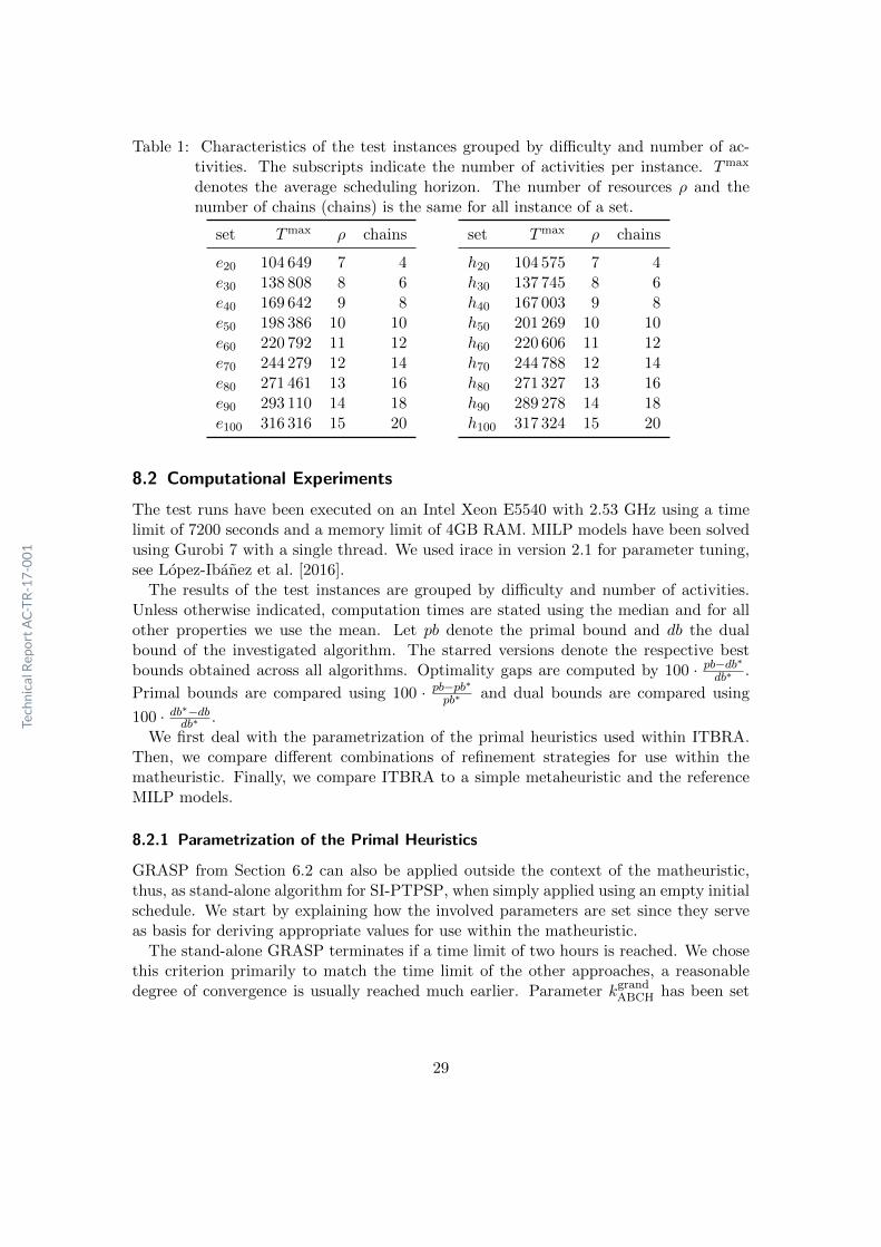
Table 1: Characteristics of the test instances grouped by difficulty and number of ac-tivities. The subscripts indicate the number of activities per instance. Tmax

denotes the average scheduling horizon. The number of resources ρ and thenumber of chains (chains) is the same for all instance of a set.

set Tmax ρ chains

e20 104 649 7 4e30 138 808 8 6e40 169 642 9 8e50 198 386 10 10e60 220 792 11 12e70 244 279 12 14e80 271 461 13 16e90 293 110 14 18e100 316 316 15 20

set Tmax ρ chains

h20 104 575 7 4h30 137 745 8 6h40 167 003 9 8h50 201 269 10 10h60 220 606 11 12h70 244 788 12 14h80 271 327 13 16h90 289 278 14 18h100 317 324 15 20

8.2 Computational Experiments

The test runs have been executed on an Intel Xeon E5540 with 2.53 GHz using a timelimit of 7200 seconds and a memory limit of 4GB RAM. MILP models have been solvedusing Gurobi 7 with a single thread. We used irace in version 2.1 for parameter tuning,see Lopez-Ibanez et al. [2016].

The results of the test instances are grouped by difficulty and number of activities.Unless otherwise indicated, computation times are stated using the median and for allother properties we use the mean. Let pb denote the primal bound and db the dualbound of the investigated algorithm. The starred versions denote the respective bestbounds obtained across all algorithms. Optimality gaps are computed by 100 · pb−db∗db∗ .

Primal bounds are compared using 100 · pb−pb∗pb∗ and dual bounds are compared using

100 · db∗−dbdb∗ .We first deal with the parametrization of the primal heuristics used within ITBRA.

Then, we compare different combinations of refinement strategies for use within thematheuristic. Finally, we compare ITBRA to a simple metaheuristic and the referenceMILP models.

8.2.1 Parametrization of the Primal Heuristics

GRASP from Section 6.2 can also be applied outside the context of the matheuristic,thus, as stand-alone algorithm for SI-PTPSP, when simply applied using an empty initialschedule. We start by explaining how the involved parameters are set since they serveas basis for deriving appropriate values for use within the matheuristic.

The stand-alone GRASP terminates if a time limit of two hours is reached. We chosethis criterion primarily to match the time limit of the other approaches, a reasonabledegree of convergence is usually reached much earlier. Parameter kgrand

ABCH has been set

29


to 8 for all benchmark instances. We applied irace to determine this value. However, itturned out that the performance of our GRASP is very robust against changes to kgrand

ABCH.For the GRASP embedded in ITBRA we imposed a time limit of 300 seconds and

a maximal number of 10,000 iterations without improvement. The latter is set highenough to be non-restrictive in most cases but avoid wasting time if the algorithm alreadyconverged sufficiently. The values of the parameters kgrand

GCH and kgrandABCH of the embedded

GRASP have been determined experimentally starting with the values from the stand-alone variant. For the parameter kgrand

GCH we first assumed a value of kgrandGCH = 5 ·kgrand

ABCH asall activity chains in the test instances consist of five activities. Afterwards, we fine-tunedthese parameters by iterative adjustment. The parameter kgrand

ABCH is set to 6 and kgrandGCH is

set to 35. The randomization itself is based on a fixed seed. Tests showed that the chosentermination criteria provide a reasonable balance between result quality and executionspeed. Objective values obtained from the embedded GRASP are on average only 0.21%larger tan those obtained from the stand-alone variant. The embedded GRASP provideson average solutions with 16.7% smaller objective value than ABCH.

The local search uses a best improvement strategy. Preliminary experiments confirmedthat this strategy works slightly better than a first improvement strategy since the aggre-gation in terms of activity blocks typically results in only few moves with improvementpotential. For the same reason the local optimum is usually reached after a few itera-tions. Thus, the overhead of the best improvement strategy is not that large. The locallyoptimal solutions obtained by the best improvement strategy, however, turned out topay off in terms of a better average quality that is achieved. Tests with irace confirmedthis observation, although the differences are quite small. However, for instances withdifferent properties this might not be the case. For a larger number of activity blocks afirst improvement strategy might be superior.

8.2.2 Comparison of Bucket Refinement Strategies

Due to the large number of possible combinations of refinement techniques (includ-ing further ones not presented in this work) we did not test every variant. Instead,we employed a local search strategy to identify good options. Experiments with thematheuristic terminate if optimality is proven or the time limit of two hours is reached.

We started with variant ASEL,B,UR and then step by step investigated the impactof exchanging each of the three parts, making use of statistical tests. It turned out thatthe best refinement strategies are VDUE,B,CPR and VDUE,SET+B,CPR. In additionto the these variants we also consider ASEL,B,UR and the best strategy based on AIGS(AIGS,SET,CPR) in the following. The former mainly serves as naıve reference strategy.The latter is used to discuss certain particularities of the bucket refinement process. Weshortly summarize the made observations here and refer to Jatschka [2017] for a moredetailed discussion.

We compared the four strategies in a pairwise fashion checking the assumption thatone strategy yields smaller optimality gaps than the other by a one-tailed Wilcoxonrank-sum test with a significance level of 0.05 per difficulty setting and in total. Allconsidered algorithms perform significantly better than the reference strategy on both

30


Table 2: Comparison of selected bucket refinement strategies. We consider the averageoptimality gaps (gap), the number of solved instances (opt) and the mediancomputation times (t). Entries marked with “tl” indicate that the experimentterminated due to the time limit. The summary is obtained by aggregatingover the preceding rows using the same function as for the respective column.

ASEL AIGS VDUE VDUEB SET B SET+B

UR CPR CPR CPR

set gap[%] opt t[s] gap[%] opt t[s] gap[%] opt t[s] gap[%] opt t[s]

e20 0.0 15 12 0.0 15 13 0.0 15 27 0.0 15 13e30 0.6 14 219 0.6 14 36 0.0 15 91 0.6 14 66e40 5.3 10 836 4.3 10 268 4.9 10 200 5.6 10 160e50 1.1 14 189 1.1 14 220 0.0 15 183 0.0 15 105e60 1.2 14 82 1.2 14 54 1.2 14 100 1.2 14 78e70 2.1 8 6957 1.2 11 2664 0.4 13 742 0.3 14 528e80 2.0 7 tl 1.7 9 1687 0.8 10 1197 0.4 13 266e90 1.7 6 tl 1.6 8 4090 1.6 6 tl 1.5 9 1908e100 0.9 5 tl 1.3 6 tl 0.7 7 tl 1.2 8 4740summary 1.7 93 836 1.4 101 268 1.1 105 200 1.2 112 160

h20 0.0 15 17 0.0 15 10 0.0 15 22 0.0 15 20h30 11.4 9 4341 8.0 10 1726 6.4 12 1860 6.4 12 985h40 14.4 4 tl 10.7 6 tl 9.5 6 tl 8.9 7 tlh50 18.3 2 tl 18.7 3 tl 17.0 4 tl 18.2 4 tlh60 18.0 1 tl 17.5 3 tl 17.6 3 tl 16.4 4 tlh70 21.9 0 tl 21.0 0 tl 21.2 0 tl 20.8 3 tlh80 13.0 1 tl 12.9 1 tl 13.0 1 tl 12.6 2 tlh90 11.1 1 tl 10.9 1 tl 10.4 1 tl 10.6 1 tlh100 10.6 0 tl 10.6 0 tl 10.6 0 tl 10.6 0 tlsummary 13.2 33 tl 12.3 39 tl 11.7 42 tl 11.6 48 tl

instance groups and also in total. The two VDUE variants outperform AIGS on the easyset of instances and in total. However, VDUE,B,CPR is not significantly better than theAIGS variant on the hard set of instances. The VDUE algorithms perform quite similarand none can be shown to work significantly better than the other.

Table 2 provides the results of the selected matheuristic variants. VDUE combinedwith SET+B and CPR is clearly the dominant strategy when taking computation timesinto account but is closely followed by VDUE,B,CPR. To discuss the results in depth wepresent more specific characteristics of the matheuristic variants in Table 3. In particular,we consider the increase in the number of buckets and the average computation timespent per iteration. The former is considered as ratio between the final and the initialnumber of buckets. The higher this ratio, the more buckets were needed to solve theinstance.

Reference strategy ASEL,B,UR generates significantly more buckets than the remain-ing approaches. This typically keeps the number of iterations low. However, this is paidfor excessively in terms of higher computation times per iteration due to the fast increasein model size. In general, the number of buckets grows too fast and unguided to obtaina successful approach.

One could expect AIGS to require the fewest buckets among the introduced strategies

31


Table 3: Comparison of the characteristics of selected bucket refinement strategies. Weconsider the ratio between the number of buckets at the start and at the end ofthe algorithm (ratioB), the average number of iterations (nit), and the averagecomputation time spent per iteration (tit). Column |Binit| provides the averagenumber of buckets contained in the initial bucket partitioning. The summaryis obtained by aggregating over the preceding rows using the same function asfor the respective column.

ASEL AIGS VDUE VDUEB SET B SET+B

UR CPR CPR CPR

set |Binit| ratioB nit tit[s] ratioB nit tit[s] ratioB nit tit[s] ratioB nit tit[s]

e20 43 4.73 9 5 2.73 5 2 1.93 16 2 1.69 9 2e30 44 7.30 9 85 5.77 9 62 2.89 24 17 2.91 16 22e40 47 7.14 7 454 5.75 7 330 2.99 19 158 2.91 13 191e50 45 8.53 7 152 10.13 9 147 2.83 15 25 2.87 12 33e60 49 5.30 4 218 5.09 5 189 2.50 11 72 2.30 6 81e70 49 10.18 6 573 8.25 7 395 3.59 18 89 3.52 12 103e80 52 7.45 4 629 7.01 5 380 3.35 13 131 3.23 9 118e90 52 6.94 3 809 6.08 4 565 3.54 11 270 3.53 8 235e100 58 7.69 3 951 6.62 4 708 3.99 13 266 3.75 9 312summary 48 7.25 6 431 6.38 6 309 3.07 16 114 2.97 10 122

h20 43 4.25 8 8 3.73 8 6 1.93 17 3 2.00 13 3h30 44 6.84 9 418 6.13 9 295 3.08 23 121 3.37 19 109h40 43 6.98 6 924 6.63 8 621 3.39 17 276 3.29 12 313h50 48 5.27 3 1812 4.90 5 1160 2.93 11 743 3.06 9 820h60 44 5.49 2 1926 6.22 5 1166 3.50 11 803 3.59 9 855h70 48 4.86 1 2629 3.96 3 2611 3.08 7 1280 3.17 6 1332h80 49 4.94 1 2362 4.97 3 1489 3.01 7 1043 3.15 5 1112h90 54 4.97 1 2239 4.61 3 1538 3.04 6 1017 3.22 5 1161h100 55 4.96 1 2617 4.79 3 1648 2.86 4 1287 3.02 4 1430summary 48 5.40 4 1659 5.10 5 1170 2.98 11 730 3.10 9 793

32


due to the potentially small number of refinement candidates. However, using onlybuckets related to activities scheduled by GCH turned out to be too restrictive. Thisstrategy causes some important splits to be delayed until the bucket partitioning is ratherfine-grained.

VDUE is again a strategy that can be expected to generate only few new buckets periteration. However, compared to AIGS their choice appears to be much more meaningful.Nevertheless, splitting only few buckets leads to a high number of iterations. Fortunately,this is not too problematic due to the small computation times per iteration. Identifyingsplitting positions with the pure binary strategy leads to only few bucket splits whichproves to be beneficial. As SET+B typically selects more candidates, one could expectthis strategy to be inferior. However, this is compensated for by incorporating moreinformation obtained from the TBR solution.

In general, it can be observed that the number of applied splits has a strong influenceon performance. However, the quality of the bucket refinement is also very important.For an illustration see Fig. 5. As mentioned before, the large number of buckets generatedby ASEL raises the computation time within a few iterations to a problematic levelcausing an overall bad performance. VDUE,B,CPR features the smallest increase inbuckets but requires more iterations to converge. Here it becomes clearly visible thatSET+B excels by incorporating more knowledge for making its decision.

Finally, we also want to discuss the properties of the remaining variants in excerpts.Fig. 6 shows a comparison of the average number of iterations and the average finalnumber of buckets for a broad selection of refinement strategies on the set of easy in-stances with 30 activities. A successful approach is typically characterized by being ableto solve an instance by refining only relatively few buckets. Variants that generate manybuckets within few iterations usually do not work well. Observe that ASEL and theAIGS variants are all located in the upper half of the figure. The superior strategiesare situated near the bottom. It is also clearly visible that SET+B allows to solve aninstance in fewer iterations than the pure binary variant. UR and BR are able to solvean instance using fewer buckets and iterations than CPR. This is a peculiarity of thesmall instances considered here that does not generalize to the larger ones.

8.2.3 Comparing ITBRA to Other Algorithms

We start by comparing the matheuristic to the stand-alone GRASP, see Table 4. ITBRAis in general able to provide better results. However, when dealing with the most difficultinstances, it is sometimes the case that the matheuristic only completes very few itera-tions and GRASP is able to compute a slightly better solution. As the number of activ-ities increases, ITBRA struggles more and more to improve upon the initially obtainedprimal bound. This is caused by the originally high computation times per iterationthat prevent the algorithm from reaching a sufficient degree of convergence. Remember,however, that ITBRA also puts much effort in determining good lower bounds whichGRASP cannot provide at all. In the remainder of this section we compare ITBRA tothe compact reference models DEF and TIF.

DEF was not able to find a primal solution for any instance but at least always

33


0 10 20 30 40 50 600

200

400

600

800

iterations

buckets

0

500

1,000

1,500

2,000

2,500

computation

time

buckets

computation time

(a) VDUE,SET+B,CPR

0 10 20 30 40 50 600

200

400

600

800

iterations

buckets

0

500

1,000

1,500

2,000

2,500

computation

time

buckets

computation time

(b) VDUE,B,CPR

0 10 20 30 40 50 600

200

400

600

800

iterations

buckets

0

500

1,000

1,500

2,000

2,500

computation

time

buckets

computation time

(c) ASEL,B,UR

Figure 5: Comparison of the relation between computation time and increase in thenumber of buckets for the same e40 instance when using different bucket re-finement strategies.

34


Table 4: Comparison of the best found refinement strategies with GRASP. For eachalgorithm the average gaps to the best primal bound (gap), the standard de-viation of the gaps (σ), and the median computation times (t) are presented.Entries marked with “tl” indicate the termination of the experiment due to thetime limit. For GRASP, we also provide the number of instances for which afeasible solution could be computed (feas). For the calculation of the gaps weconsidered only instances for which all algorithms were able to compute a pri-mal bound. The summary is obtained by aggregating over the preceding rowsusing the same function as for the respective column.

VDUE VDUEB SET+B

CPR CPR GRASP

set gap[%] σ t[s] gap[%] σ t[s] gap[%] σ feas

e20 0.0 0.0 27 0.0 0.0 13 38.6 17.3 12e30 0.0 0.0 91 0.6 2.1 66 28.0 16.0 14e40 3.5 7.4 200 4.2 7.4 160 12.6 7.7 15e50 0.0 0.0 183 0.0 0.0 105 7.8 8.0 15e60 0.8 2.9 100 0.8 2.9 78 3.4 4.6 15e70 0.4 1.6 742 0.3 1.0 528 3.8 3.9 15e80 0.5 1.1 1197 0.1 0.4 266 2.2 3.7 15e90 0.8 1.0 tl 0.7 1.0 1908 0.9 1.0 15e100 0.2 0.5 tl 0.7 1.5 4740 1.3 2.1 15summary 0.7 1.6 200 0.8 1.8 160 11.0 7.1 131

h20 0.0 0.0 22 0.0 0.0 20 23.3 12.7 12h30 5.9 13.1 1860 5.9 13.1 985 34.9 11.9 15h40 6.5 8.2 tl 5.9 8.1 tl 21.6 11.6 15h50 6.6 7.5 tl 7.6 7.9 tl 10.6 7.1 15h60 6.9 5.8 tl 5.6 5.5 tl 8.4 5.6 15h70 2.7 3.2 tl 2.2 3.3 tl 4.5 5.9 15h80 1.3 2.9 tl 0.9 2.0 tl 1.1 2.9 15h90 2.0 3.4 tl 2.2 4.1 tl 2.6 6.0 15h100 1.0 0.9 tl 1.0 0.9 tl 0.1 0.5 15summary 3.7 5.0 tl 3.5 5.0 tl 11.9 7.1 132

35


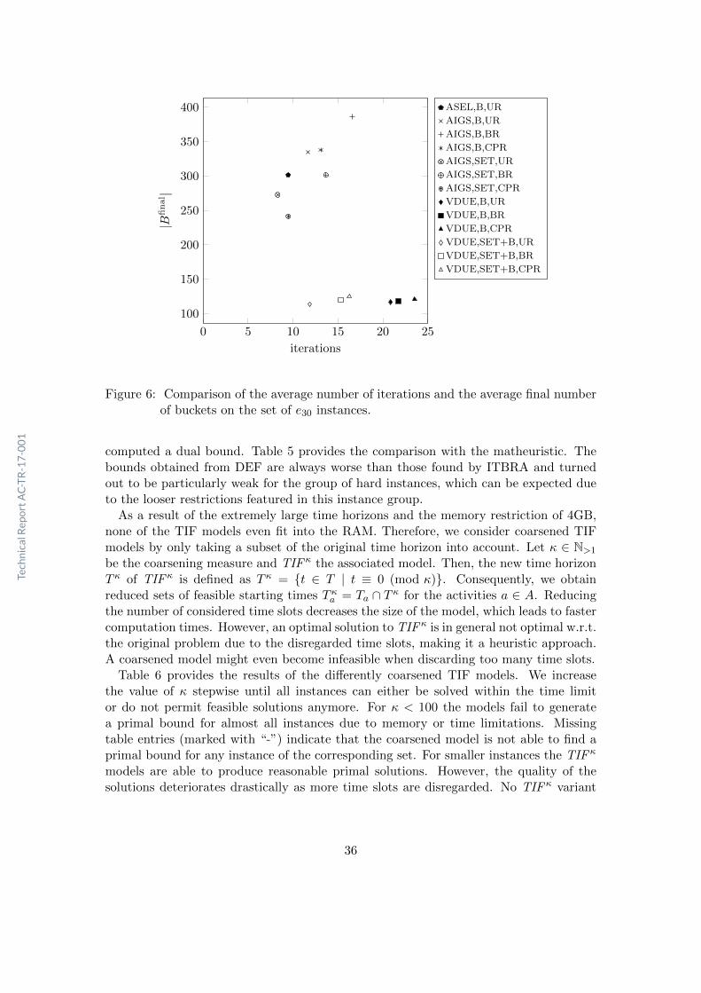
0 5 10 15 20 25

100

150

200

250

300

350

400

iterations

|Bfinal |

ASEL,B,UR

AIGS,B,UR

AIGS,B,BR

AIGS,B,CPR

AIGS,SET,UR

AIGS,SET,BR

AIGS,SET,CPR

VDUE,B,UR

VDUE,B,BR

VDUE,B,CPR

VDUE,SET+B,UR

VDUE,SET+B,BR

VDUE,SET+B,CPR

Figure 6: Comparison of the average number of iterations and the average final numberof buckets on the set of e30 instances.

computed a dual bound. Table 5 provides the comparison with the matheuristic. Thebounds obtained from DEF are always worse than those found by ITBRA and turnedout to be particularly weak for the group of hard instances, which can be expected dueto the looser restrictions featured in this instance group.

As a result of the extremely large time horizons and the memory restriction of 4GB,none of the TIF models even fit into the RAM. Therefore, we consider coarsened TIFmodels by only taking a subset of the original time horizon into account. Let κ ∈ N>1

be the coarsening measure and TIFκ the associated model. Then, the new time horizonT κ of TIFκ is defined as T κ = {t ∈ T | t ≡ 0 (mod κ)}. Consequently, we obtainreduced sets of feasible starting times T κa = Ta ∩ T κ for the activities a ∈ A. Reducingthe number of considered time slots decreases the size of the model, which leads to fastercomputation times. However, an optimal solution to TIFκ is in general not optimal w.r.t.the original problem due to the disregarded time slots, making it a heuristic approach.A coarsened model might even become infeasible when discarding too many time slots.

Table 6 provides the results of the differently coarsened TIF models. We increasethe value of κ stepwise until all instances can either be solved within the time limitor do not permit feasible solutions anymore. For κ < 100 the models fail to generatea primal bound for almost all instances due to memory or time limitations. Missingtable entries (marked with “-”) indicate that the coarsened model is not able to find aprimal bound for any instance of the corresponding set. For smaller instances the TIFκ

models are able to produce reasonable primal solutions. However, the quality of thesolutions deteriorates drastically as more time slots are disregarded. No TIFκ variant

36


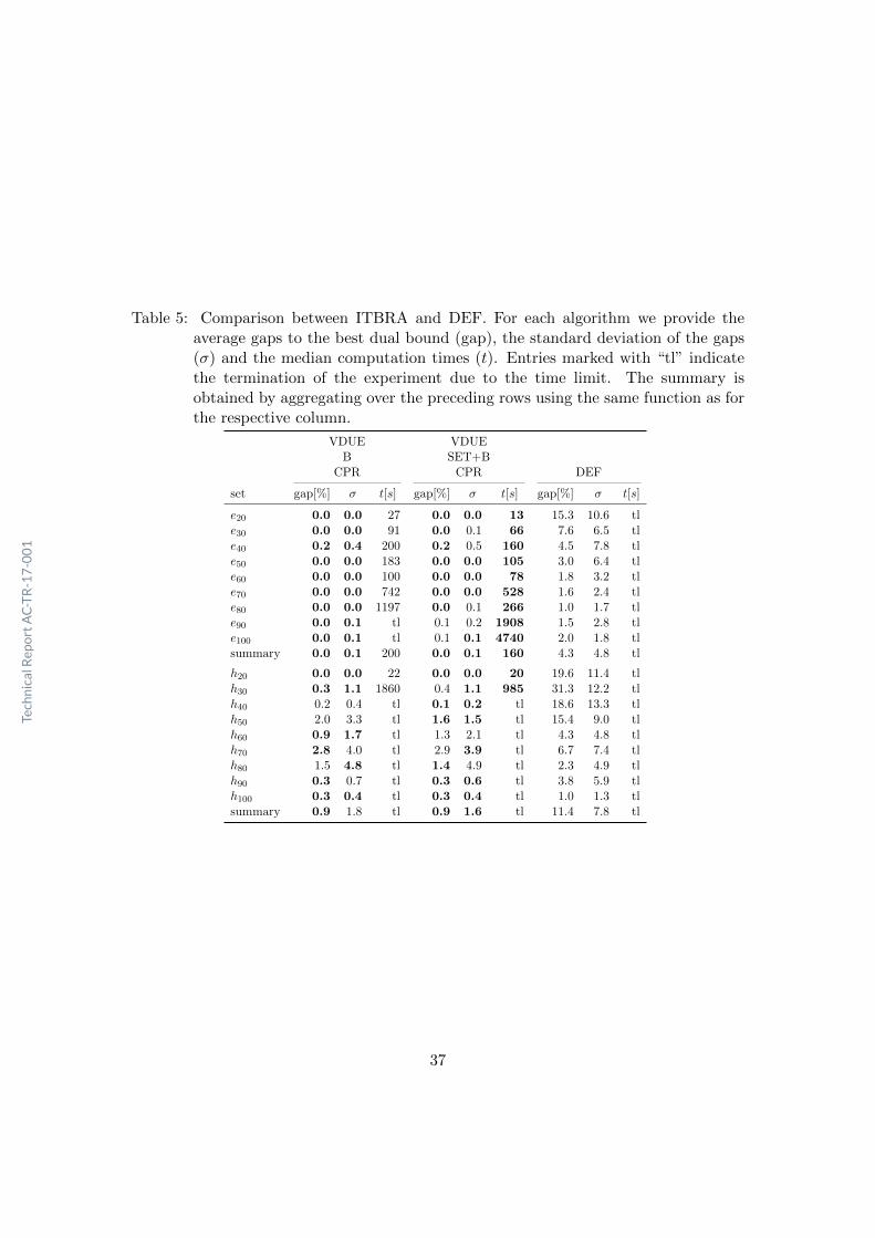
Table 5: Comparison between ITBRA and DEF. For each algorithm we provide theaverage gaps to the best dual bound (gap), the standard deviation of the gaps(σ) and the median computation times (t). Entries marked with “tl” indicatethe termination of the experiment due to the time limit. The summary isobtained by aggregating over the preceding rows using the same function as forthe respective column.

VDUE VDUEB SET+B

CPR CPR DEF

set gap[%] σ t[s] gap[%] σ t[s] gap[%] σ t[s]

e20 0.0 0.0 27 0.0 0.0 13 15.3 10.6 tle30 0.0 0.0 91 0.0 0.1 66 7.6 6.5 tle40 0.2 0.4 200 0.2 0.5 160 4.5 7.8 tle50 0.0 0.0 183 0.0 0.0 105 3.0 6.4 tle60 0.0 0.0 100 0.0 0.0 78 1.8 3.2 tle70 0.0 0.0 742 0.0 0.0 528 1.6 2.4 tle80 0.0 0.0 1197 0.0 0.1 266 1.0 1.7 tle90 0.0 0.1 tl 0.1 0.2 1908 1.5 2.8 tle100 0.0 0.1 tl 0.1 0.1 4740 2.0 1.8 tlsummary 0.0 0.1 200 0.0 0.1 160 4.3 4.8 tl

h20 0.0 0.0 22 0.0 0.0 20 19.6 11.4 tlh30 0.3 1.1 1860 0.4 1.1 985 31.3 12.2 tlh40 0.2 0.4 tl 0.1 0.2 tl 18.6 13.3 tlh50 2.0 3.3 tl 1.6 1.5 tl 15.4 9.0 tlh60 0.9 1.7 tl 1.3 2.1 tl 4.3 4.8 tlh70 2.8 4.0 tl 2.9 3.9 tl 6.7 7.4 tlh80 1.5 4.8 tl 1.4 4.9 tl 2.3 4.9 tlh90 0.3 0.7 tl 0.3 0.6 tl 3.8 5.9 tlh100 0.3 0.4 tl 0.3 0.4 tl 1.0 1.3 tlsummary 0.9 1.8 tl 0.9 1.6 tl 11.4 7.8 tl

37


is able to find a primal solution for all instances. When using a small value for κ, manyinstances cannot be solved due to the time limit. For larger κ-values we can solve moreinstances but at the cost of much larger gaps. Moreover, as we reduce the precisioneven further, the models start to become infeasible. The number of infeasible instancesstrongly increases for κ ≥ 10000 and the few instances that still permit feasible solutionsfeature gaps of over 120%. Therefore, further increasing the value of κ does not seemmeaningful. It appears that there does not exist an appropriate value for κ allowinga reasonable balance between computation time and result quality. Due to the manymissing entries we decided to use median instead of average gaps in the summary table.

According to our experiments the best variants are those with κ = 1000 and κ = 2000,respectively. The former provides better solutions but the latter is able to find morefeasible solutions. For some instances the coarsened TIF variants even find better primalsolutions than the matheuristic. Especially for instance sets h40, h50, and h60 we obtaina high number of good solutions s.t. also the median gaps are smaller here. Overall,however, ITBRA still provides the better results. Moreover, recall that the TIFκ modelscan only provide heuristic solutions and no dual bounds.

Last but not least, we also investigated the use of disaggregated precedence constraints(see Artigues [2017]) but this did not lead to significant improvements.

9 Conclusions

In this work we considered a matheuristic, referred to as iterative time-bucket refine-ment algorithm (ITBRA), intended for solving a resource-constrained project schedulingproblem (RCPSP) that requires scheduling in high resolution. We proposed a relaxationfor the original problem based on aggregating consecutive integral time points into so-called time-buckets. Exploiting this relaxation we constructed a matheuristic that solvesthis relaxation based on iteratively refined bucket partitionings. Moreover, we heuris-tically derive primal bounds incorporating information from the relaxed solution. Thematheuristic then attempts to close the gap between dual bounds obtained from therelaxation and primal bounds determined by (meta-)heuristics. The crucial part of thisapproach is how to determine the subsequent (more refined) bucket partitioning forthe next iteration. We considered a variety of strategies and investigated them on anovel benchmark set motivated by an application arising in particle therapy for cancertreatment.

Our experiments indicate that it is most critical to limit the increase in the number ofbuckets. However, the quality of the applied bucket splits has a substantial impact onthe convergence speed. Strategy VDUE,SET+B,CPR turned out to work best in thisrespect.

The matheuristic works better than a simple greedy randomized adaptive search pro-cedure (GRASP) on all instance sets except for the most difficult one. There it failsto complete a sufficient number of iterations to make reasonable improvements to theprimal bound.

ITBRA clearly outperforms the compact mixed integer linear programming (MILP)

38


Table 6: Comparison of differently coarsened TIF models with ITBRA. We provide themedian gaps to the best primal bound of the original problem (gap) and themedian computation times (t). Missing entries (“-”) indicate that the coarsenedmodel is not able to find a primal bound for any instance of the correspondingset. Moreover, for each instance set we indicate the number of optimally (optc)and feasibly (feas) solved instances w.r.t. the coarsened model. Column infeasdenotes the number of instances with proven infeasible model. Finally, weindicate the number of instances that terminated due to the time limit (tl) orthe memory limit (ml), respectively. The summary is obtained by aggregatingover the preceding rows using the same function as for the respective column.

VDUE VDUEB SET+B

TIF100 TIF200 TIF1000 TIF2000 TIF10000 CPR CPR

set gapmed [%] t[s] gapmed [%] t[s] gapmed [%] t[s] gapmed [%] t[s] gapmed [%] t[s] gapmed [%] t[s] gapmed [%] t[s]

e20 0.3 15 0.6 4 21.7 <1 24.0 <1 - - 0.0 27 0.0 13e30 0.1 310 0.4 58 4.0 4 18.3 2 - - 0.0 91 0.0 66e40 0.3 2940 0.5 698 3.8 40 12.3 6 - - 0.0 200 0.0 160e50 0.2 409 0.4 113 1.9 17 6.4 5 - <1 0.0 183 0.0 105e60 0.3 5569 0.4 839 2.4 52 4.7 21 - <1 0.0 100 0.0 78e70 14.3 tl 0.3 2713 1.9 165 4.7 77 - <1 0.0 742 0.0 528e80 - tl 0.3 5630 1.7 292 3.4 108 - <1 0.0 1197 0.0 266e90 - tl - tl 0.9 555 3.0 327 - 1 0.0 tl 0.0 1908e100 - tl - tl 1.8 652 4.0 263 - 6 0.0 tl 0.0 4740summary 0.3 5569 0.4 839 1.9 52 4.7 21 - <1 0.0 200 0.0 160

h20 0.4 39 0.5 8 6.4 1 19.8 <1 - <1 0.0 22 0.0 20h30 11.8 6106 1.0 1129 11.1 42 24.6 13 - - 0.0 1860 0.0 985h40 35.4 tl 0.6 tl 5.5 227 13.7 65 - <1 3.9 tl 3.2 tlh50 - tl - tl 0.0 2815 9.5 381 - <1 3.5 tl 3.9 tlh60 - tl 8.9 tl 2.3 1532 7.0 940 - <1 9.2 tl 6.5 tlh70 - tl - tl 14.3 tl 10.4 3052 82.5 <1 1.6 tl 0.0 tlh80 - tl - tl 5.0 tl 12.1 tl 77.0 3 0.0 tl 0.0 tlh90 - tl - tl 9.0 tl 14.2 tl 93.8 8 0.3 tl 0.3 tlh100 - tl - tl 39.6 tl 22.7 tl - 16 1.2 tl 1.2 tlsummary - tl - tl 6.4 2815 13.7 940 - <1 1.2 tl 0.3 tl

TIF 100 TIF 200 TIF 1000 TIF 2000 TIF 10000

set optc feas infeas tl ml optc feas infeas tl optc feas infeas tl optc feas infeas tl optc feas infeas tl

e20 15 15 0 0 0 15 15 0 0 15 15 0 0 13 13 2 0 0 0 15 0e30 15 15 0 0 0 15 15 0 0 15 15 0 0 15 15 0 0 0 0 15 0e40 9 12 0 6 0 12 14 0 3 15 15 0 0 15 15 0 0 0 0 15 0e50 13 14 0 2 0 14 14 0 1 15 15 0 0 15 15 0 0 2 2 13 0e60 9 9 0 6 0 14 15 0 1 15 15 0 0 15 15 0 0 6 6 9 0e70 6 9 0 9 0 12 14 0 3 15 15 0 0 15 15 0 0 2 2 13 0e80 3 3 0 12 0 9 11 0 6 15 15 0 0 15 15 0 0 7 7 8 0e90 0 0 0 13 2 6 7 0 9 14 14 0 1 14 15 0 1 4 4 11 0e100 1 1 0 8 6 4 5 0 11 13 15 0 2 15 15 0 0 2 2 13 0summary 71 78 0 56 8 101 110 0 34 132 134 0 3 132 133 2 1 23 23 112 0

h20 15 15 0 0 0 15 15 0 0 15 15 0 0 15 15 0 0 2 2 13 0h30 8 12 0 7 0 14 15 0 1 15 15 0 0 14 14 1 0 0 0 15 0h40 4 9 0 11 0 8 12 0 7 15 15 0 0 15 15 0 0 5 5 10 0h50 1 4 0 14 0 4 7 0 11 12 15 0 3 15 15 0 0 6 6 9 0h60 0 0 0 15 0 2 9 0 13 9 15 0 6 14 15 0 1 6 6 9 0h70 0 0 0 15 0 0 1 0 15 4 10 0 11 10 15 0 5 8 8 7 0h80 0 0 0 11 4 1 4 0 14 5 11 0 10 4 15 0 11 9 9 6 0h90 0 0 0 12 3 1 1 0 14 4 12 0 11 6 12 0 9 8 8 7 0h100 0 0 0 1 14 0 0 0 15 1 8 0 14 0 11 0 15 5 5 10 0summary 28 40 0 86 21 45 64 0 90 80 116 0 55 93 127 1 41 49 49 86 0

39


formulations. The considered discrete-event formulation (DEF) is only capable of com-puting dual bounds for all of our benchmark instances and the considered time-indexedformulation (TIF) cannot even be solved due to its model size. Variants of TIF basedon a coarsened time horizon are manageable but become infeasible once too many timepoints are disregarded. For some instances good primal solutions could be obtained butthere exists no coarsening factor that works well in general by providing a good balancebetween model size and result quality.

We primarily focused on MILP-based algorithms here. Another well-known exacttechnique often used to deal with scheduling problems is constraint programming (CP).In a more comprehensive study it appears to be interesting to compare our matheuristicalso to a suitable CP approach. Moreover, it might also be relevant to consider CPtechniques within ITBRA to improve its performance. In general the (meta-)heuristicscurrently used within the matheuristic are rather simple. In particular, they suffer fromthe effects of fixing the time lags which prevents them from considering a large varietyof possible solutions. This is a crucial part of the matheuristic for which more elaboratetechniques should be identified and tested.

In the computational study we investigated the power of our algorithm on a ratherspecific set of benchmark instances. The fundamental approach, however, is in principlemuch more generally applicable to problems that require scheduling in high resolution.To verify this a more diversified set of benchmark instances, originating from differ-ent application domains, has to be considered. Of course this requires adjusted MILPformulations and adapted as well as novel bucket refinement strategies.

Acknowledgments

We thank EBG MedAustron GmbH, Wiener Neustadt, Austria, for the collaboration onparticle therapy patient scheduling and partially funding this work.

References

C. Artigues. On the strength of time-indexed formulations for the resource-constrainedproject scheduling problem. Operations Research Letters, 45(2):154 – 159, 2017.

C. Artigues and E. Hebrard. Mip relaxation and large neighborhood search for a multi-mode resource-constrained multi-project scheduling problem. In G. Kendall, B. Mc-Collum, and G. Venden Berghe, editors, In proceedings of the 6th MultidisciplinaryInternational Conference on Scheduling : Theory and Applications (MISTA 2013),27–30 Aug 2013, Ghent, Belgium, pages 815–819, 2013.

C. Artigues, S. Demassey, and E. Neron. Resource-Constrained Project Scheduling: Mod-els, Algorithms, Extensions and Applications. Wiley-ISTE, 2008.

C. Artigues, P. Brucker, S. Knust, O. Kone, and P. Lopez. A note on “event-based

40


MILP models for resource-constrained project scheduling problems”. Computers andOperations Research, 40(4):1060–1063, 2013.

P. Baptiste and R. Sadykov. On scheduling a single machine to minimize a piecewiselinear objective function: A compact MIP formulation. Naval Research Logistics, 56(6):487–502, 2009.

G. Baydoun, A. Haıt, R. Pellerin, B. Clement, and G. Bouvignies. A rough-cut capacityplanning model with overlapping. OR Spectrum, 38(2):335–364, 2016.

T. Berthold, S. Heinz, M. E. Lubbecke, R. H. Mohring, and J. Schulz. A constraintinteger programming approach for resource-constrained project scheduling. In Inter-national Conference on Integration of Artificial Intelligence (AI) and Operations Re-search (OR) Techniques in Constraint Programming, pages 313–317. Springer, 2010.

L. Bianco and M. Caramia. A new lower bound for the resource-constrained projectscheduling problem with generalized precedence relations. Computers & OperationsResearch, 38(1):14–20, 2011a.

L. Bianco and M. Caramia. Minimizing the completion time of a project under re-source constraints and feeding precedence relations: a lagrangian relaxation basedlower bound. 4OR, 9(4):371–389, 2011b.

L. Bianco and M. Caramia. An exact algorithm to minimize the makespan in projectscheduling with scarce resources and generalized precedence relations. European Jour-nal of Operational Research, 219(1):73–85, 2012.

L. P. Bigras, M. Gamache, and G. Savard. Time-indexed formulations and the totalweighted tardiness problem. INFORMS Journal on Computing, 20(1):133–142, 2008.

N. Boland, R. Clement, and H. Waterer. A Bucket Indexed Formulation for Nonpre-emptive Single Machine Scheduling Problems. INFORMS Journal on Computing, 28(1):14–30, 2016.

N. Boland, M. Hewitt, L. Marshall, and M. Savelsbergh. The continuous-time servicenetwork design problem. Operations Research, 65(5):1303–1321, 2017.

C. Bron and J. Kerbosch. Algorithm 457: Finding all cliques of an undirected graph.Communications of the ACM, 16(9):575–577, 1973.

P. Brucker, A. Drexl, R. Mohring, K. Neumann, and E. Pesch. Resource-constrainedproject scheduling: Notation, classification, models, and methods. European journalof operational research, 112(1):3–41, 1999.

J. Carlier, A. Moukrim, and A. Sahli. Lower bounds for the Event Scheduling Problemwith Consumption and Production of Resources. Discrete Applied Mathematics, toappear. available at https://doi.org/10.1016/j.dam.2016.05.021.

41


F. Cazals and C. Karande. A note on the problem of reporting maximal cliques. Theo-retical Computer Science, 407(1–3):564 – 568, 2008. ISSN 0304-3975.

F. Clautiaux, S. Hanafi, R. Macedo, M. Voge, and C. Alves. Iterative aggregationand disaggregation algorithm for pseudo-polynomial network flow models with sideconstraints. European Journal of Operational Research, 258(2):467–477, 2017.

S. Dash, O. Gunluk, A. Lodi, and A. Tramontani. A time bucket formulation for thetraveling salesman problem with time windows. INFORMS Journal on Computing,24(1):132–147, 2012.

S. Demassey, C. Artigues, and P. Michelon. Constraint-propagation-based cuttingplanes: An application to the resource-constrained project scheduling problem. IN-FORMS Journal on Computing, 17(1):52–65, 2005.

E. L. Demeulemeester and W. S. Herroelen. A Branch-and-Bound Procedure for theGeneralized Resource-Constrained Project Scheduling Problem. Operations Research,45(2):201–212, 1997.

N. Dupin and E. G. Talbi. Dual Heuristics and New Lower Bounds for the ChallengeEURO/ROADEF 2010. In Matheuristics 2016 - Proceedings of the Sixth InternationalWorkshop on Model-based Metaheuristics, 4–7 Sep 2016, Brussels, Belgium, pages 60–71, 2016.

M. L. Fisher. Optimal Solution of Scheduling Problems Using Lagrange Multipliers:Part I. Operations Research, 21(5):1114–1127, 1973.

R. L. Graham, E. L. Lawler, J. K. Lenstra, and A. H. G. Rinnooy Kan. Optimizationand approximation in deterministic sequencing and scheduling: a survey. Annals ofdiscrete mathematics, 5:287–326, 1979.

F. Guerriero and L. Talarico. A solution approach to find the critical path in a time-constrained activity network. Computers & Operations Research, 37(9):1557 – 1569,2010.

J. R. Hardin, G. L. Nemhauser, and M. W. P. Savelsbergh. Strong valid inequalitiesfor the resource-constrained scheduling problem with uniform resource requirements.Discrete Optimization, 5(1):19 – 35, 2008. ISSN 1572-5286.

S. Hartmann and D. Briskorn. A survey of variants and extensions of the resource-constrained project scheduling problem. European Journal of Operational Research,207(1):1–14, 2010.

J. N. Hooker. Planning and Scheduling by Logic-Based Benders Decomposition. Oper-ations Research, 55(3):588–602, 2007.

T. Jatschka. An iterative refinement algorithm for high resolution scheduling problems.Master’s thesis, TU Wien, 2017. in preparation.

42


O. Kone, C. Artigues, P. Lopez, and M. Mongeau. Event-based MILP models forresource-constrained project scheduling problems. Computers & Operations Research,38(1):3–13, 2011.

E. L. Lawler and J. K. Lenstra. Machine Scheduling with Precedence Constraints. InI. Rival, editor, Ordered Sets, pages 655–675. Springer Netherlands, 1982.

Y. Li, O. Ergun, and G. L. Nemhauser. A dual heuristic for mixed integer programming.Operations Research Letters, 43(4):411–417, 2015.

M. Lopez-Ibanez, J. Dubois-Lacoste, L. P. Caceres, M. Birattari, and T. Stutzle. Theirace package: Iterated racing for automatic algorithm configuration. Operations Re-search Perspectives, 3:43–58, 2016.

R. Macedo, C. Alves, J. De Carvalho, F. Clautiaux, and S. Hanafi. Solving the vehi-cle routing problem with time windows and multiple routes exactly using a pseudo-polynomial model. European Journal of Operational Research, 214(3):536–545, 2011.

A. K. Mackworth. Consistency in networks of relations. Artificial intelligence, 8(1):99–118, 1977.

V. Maniezzo and A. Mingozzi. A heuristic procedure for the multi-mode project schedul-ing problem based on Benders’ decomposition. In J. Weglarz, editor, Project Schedul-ing: Recent Models, Algorithms and Applications, pages 179–196. Springer US, Boston,MA, 1999.

V. Maniezzo, T. Stutzle, and S. Voß, editors. Matheuristics: Hybridizing Metaheuristicsand Mathematical Programming. Springer US, 2010.

R. H. Mohring, A. S. Schulz, F. Stork, and M. Uetz. Solving project scheduling problemsby minimum cut computations. Management Science, 49(3):330–350, 2003.

K. Neumann, C. Schwindt, and J. Zimmermann. Project Scheduling with Time Windowsand Scarce Resources. Springer Berlin Heidelberg, 2003.

M. Palpant, C. Artigues, and P. Michelon. LSSPER: Solving the resource-constrainedproject scheduling problem with large neighbourhood search. Annals of OperationsResearch, 131(1-4):237–257, 2004.

M. G. C. Resende and C. C. Ribeiro. Greedy randomized adaptive search procedures:Advances, hybridizations, and applications. In M. Gendreau and J. Potvin, editors,Handbook of Metaheuristics, pages 283–319. Springer US, Boston, MA, 2010.

T. A. M. Toffolo, H. G. Santos, M. A. M. Carvalho, and J. A. Soares. An integerprogramming approach to the multimode resource-constrained multiproject schedulingproblem. Journal of Scheduling, 19(3):295–307, 2016.

X. Wang and A. C. Regan. Local truckload pickup and delivery with hard time windowconstraints. Transportation Research Part B: Methodological, 36(2):97–112, 2002.

43


X. Wang and A. C. Regan. On the Convergence of a New Time Window Discretiza-tion Method for the Traveling Salesman Problem with Time Window Constraints.Computers & Industrial Engineering, 56(1):161–164, 2009.

J. Westerlund, M. Hastbacka, S. Forssell, and T. Westerlund. Mixed-Time Mixed-IntegerLinear Programming Scheduling Model. Industrial & Engineering Chemistry Research,46(9):2781–2796, 2007.

44


Documents

InstituteofComputerGraphicsandAlgorithms TUWien,Vienna,Austria · A feasible solution S (also called schedule) to SI-PTPSP is a vector of values S a 2 T a assigning each activity