Instanton Floer homology and the Alexander

polynomial

P. B. Kronheimer and T. S. Mrowka1

Harvard University, Cambridge MA 02138

Massachusetts Institute of Technology, Cambridge MA 02139

Abstract. The instanton Floer homology of a knot in S3 is a vector space with acanonical mod 2 grading. It carries a distinguished endomorphism of even degree,arising from the 2-dimensional homology class represented by a Seifert surface.The Floer homology decomposes as a direct sum of the generalized eigenspaces ofthis endomorphism. We show that the Euler characteristics of these generalizedeigenspaces are the coefficients of the Alexander polynomial of the knot. Amongother applications, we deduce that instanton homology detects fibered knots.

1 Introduction

For a knot K ⊂ S3, the authors defined in [8] a Floer homology groupKHI (K), by a slight variant of a construction that appeared first in [3]. Inbrief, one takes the knot complement S3 \N◦(K) and forms from it a closed3-manifold Z(K) by attaching to ∂N(K) the manifold F × S1, where F isa genus-1 surface with one boundary component. The attaching is done insuch a way that {point}×S1 is glued to the meridian of K and ∂F×{point}is glued to the longitude. The vector space KHI (K) is then defined byapplying Floer’s instanton homology to the closed 3-manifold Z(K). Wewill recall the details in section 2. If Σ is a Seifert surface for K, then thereis a corresponding closed surface Σ in Z(K), formed as the union of Σ andone copy of F . The homology class σ = [Σ] in H2(Z(K)) determines anendomorphism µ(σ) on the instanton homology of Z(K), and hence also anendomorphism of KHI (K). As was shown in [8], and as we recall below, the

1The work of the first author was supported by the National Science Foundationthrough NSF grant number DMS-0405271. The work of the second author was supportedby NSF grants DMS-0206485, DMS-0244663 and DMS-0805841.

arX

iv:0

907.

4639

v2 [

mat

h.G

T]

3 J

un 2

010

2

Figure 1: Knots K+, K− and K0 differing at a single crossing.

generalized eigenspaces of µ(σ) give a direct sum decomposition,

KHI (K) =

g⊕j=−g

KHI (K, j). (1)

Here g is the genus of the Seifert surface. In this paper, we will define acanonical Z/2 grading on KHI (K), and hence on each KHI (K, j), so thatwe may write

KHI (K, j) = KHI 0(K, j)⊕KHI 1(K, j).

This allows us to define the Euler characteristic χ(KHI (K, j)) as the differ-ence of the ranks of the even and odd parts. The main result of this paperis the following theorem.

Theorem 1.1. For any knot in S3, the Euler characteristics χ(KHI (K, j))of the summands KHI (K, j) are minus the coefficients of the symmetrizedAlexander polynomial ∆K(t), with Conway’s normalization. That is,

∆K(t) = −∑j

χ(KHI (K, j))tj .

The Floer homology group KHI (K) is supposed to be an “instanton”counterpart to the Heegaard knot homology of Ozsvath-Szabo and Ras-mussen [12, 13]. It is known that the Euler characteristic of Heegaard knothomology gives the Alexander polynomial; so the above theorem can betaken as further evidence that the two theories are indeed closely related.

The proof of the theorem rests on Conway’s skein relation for the Alexan-der polynomial. To exploit the skein relation in this way, we first extendthe definition of KHI (K) to links. Then, given three oriented knots or links

3

K+, K− and K0 related by the skein moves (see Figure 1), we establish along exact sequence relating the instanton knot (or link) homologies of K+,K− and K0. More precisely, if for example K+ and K− are knots and K0 isa 2-component link, then we will show that there is along exact sequence

· · · → KHI (K+)→ KHI (K−)→ KHI (K0)→ · · · .

(This situation is a little different when K+ and K− are 2-component linksand K0 is a knot: see Theorem 3.1.)

Skein exact sequences of this sort for KHI (K) are not new. The defi-nition of KHI (K) appears almost verbatim in Floer’s paper [3], along withoutline proofs of just such a skein sequence. See in particular part (2′) ofTheorem 5 in [3], which corresponds to Theorem 3.1 in this paper. The ma-terial of Floer’s paper [3] is also presented in [1]. The proof of the skein exactsequence which we shall describe is essentially Floer’s argument, as ampli-fied in [1], though we shall present it in the context of sutured manifolds.The new ingredient however is the decomposition (1) of the instanton Floerhomology, without which one cannot arrive at the Alexander polynomial.

The structure of the remainder of this paper is as follows. In section 2,we recall the construction of instanton knot homology, as well as instan-ton homology for sutured manifolds, following [8]. We take the opportunityhere to extend and slightly generalize our earlier results concerning theseconstructions. Section 3 presents the proof of the main theorem. Some ap-plications are discussed in section 4. The relationship between ∆K(t) andthe instanton homology of K was conjectured in [8], and the result providesthe missing ingredient to show that the KHI detects fibered knots. Theo-rem 1.1 also provides a lower bound for the rank of the instanton homologygroup:

Corollary 1.2. If the Alexander polynomial of K is∑d−d ajt

j, then the rank

of KHI (K) is not less than∑d−d |aj |.

The corollary can be used to draw conclusions about the existence ofcertain representations of the knot group in SU (2).

Acknowledgment. As this paper was being completed, the authors learnedthat essentially the same result has been obtained simultaneously by YuhanLim [9]. The authors are grateful to the referee for pointing out the errors inan earlier version of this paper, particularly concerning the mod 2 gradings.

4

2 Background

2.1 Instanton Floer homology

Let Y be a closed, connected, oriented 3-manifold, and let w → Y be ahermitian line bundle with the property that the pairing of c1(w) with someclass in H2(Y ) is odd. If E → Y is a U(2) bundle with Λ2E ∼= w, we writeB(Y )w for the space of PU (2) connections in the adjoint bundle ad(E),modulo the action of the gauge group consisting of automorphisms of Ewith determinant 1. The instanton Floer homology group I∗(Y )w is theFloer homology arising from the Chern-Simons functional on B(Y )w. Ithas a relative grading by Z/8. Our notation for this Floer group follows[8]; an exposition of its construction is in [2]. We will always use complexcoefficients, so I∗(Y )w is a complex vector space.

If σ is a 2-dimensional integral homology class in Y , then there is acorresponding operator µ(σ) on I∗(Y )w of degree −2. If y ∈ Y is a pointrepresenting the generator of H0(Y ), then there is also a degree-4 operatorµ(y). The operators µ(σ), for σ ∈ H2(Y ), commute with each other andwith µ(y). As shown in [8] based on the calculations of [10], the simultaneouseigenvalues of the commuting pair of operators (µ(y), µ(σ)) all have the form

(2, 2k) or (−2, 2k√−1), (2)

for even integers 2k in the range

|2k| ≤ |σ|.

Here |σ| denotes the Thurston norm of σ, the minimum value of −χ(Σ) overall aspherical embedded surfaces Σ with [Σ] = σ.

2.2 Instanton homology for sutured manifolds

We recall the definition of the instanton Floer homology for a balancedsutured manifold, as introduced in [8] with motivation from the Heegaardcounterpart defined in [4]. The reader is referred to [8] and [4] for backgroundand details.

Let (M,γ) be a balanced sutured manifold. Its oriented boundary is aunion,

∂M = R+(γ) ∪A(γ) ∪ (−R−(γ))

where A(γ) is a union of annuli, neighborhoods of the sutures s(γ). Todefine the instanton homology group SHI (M,γ) we proceed as follows. Let

5

([−1, 1]×T, δ) be a product sutured manifold, with T a connected, orientedsurface with boundary. The annuli A(δ) are the annuli [−1, 1]× ∂T , and wesuppose these are in one-to-one correspondence with the annuli A(γ). Weattach this product piece to (M,γ) along the annuli to obtain a manifold

M = M ∪([−1, 1]× T

). (3)

We write∂M = R+ ∪ (−R−). (4)

We can regard M as a sutured manifold (not balanced, because it has nosutures). The surface R+ and R− are both connected and are diffeomorphic.We choose an orientation-preserving diffeomorphism

h : R+ → R−

and then define Z = Z(M,γ) as the quotient space

Z = M/ ∼,

where ∼ is the identification defined by h. The two surfaces R± give a singleclosed surface

R ⊂ Z.

We need to impose a side condition on the choice of T and h in order toproceed. We require that there is a closed curve c in T such that {1} × cand {−1}×c become non-separating curves in R+ and R− respectively; andwe require further that h is chosen so as to carry {1}× c to {−1}× c by theidentity map on c.

Definition 2.1. We say that (Z, R) is an admissible closure of (M,γ) ifit arises in this way, from some choice of T and h, satisfying the aboveconditions. ♦

Remark. In [8, Definition 4.2], there was an additional requirement thatR± should have genus 2 or more. This was needed only in the contextthere of Seiberg-Witten Floer homology, as explained in section 7.6 of [8].Furthermore, the notion of closure in [8] did not require that h carry {1}× cto {−1} × c, hence the qualification “admissible” in the present paper.

In an admissible closure, the curve c gives rise to a torus S1 × c in Zwhich meets R transversely in a circle. Pick a point x on c. The closedcurve S1 × {x} lies on the torus S1 × c and meets R in a single point. Wewrite

w → Z

6

for a hermitian line bundle on Z whose first Chern class is dual to S1 ×{x}. Since c1(w) has odd evaluation on the closed surface R, the instantonhomology group I∗(Z)w is well-defined. As in [8], we write

I∗(Z|R)w ⊂ I∗(Z)w

for the simultaneous generalized eigenspace of the pair of operators

(µ(y), µ(R))

belonging to the eigenvalues (2, 2g−2), where g is the genus of R. (See (2).)

Definition 2.2. For a balanced sutured manifold (M,γ), the instantonFloer homology group SHI (M,γ) is defined to be I∗(Z|R)w, where (Z, R) isany admissible closure of (M,γ). ♦.

It was shown in [8] that SHI (M,γ) is well-defined, in the sense that anytwo choices of T or h will lead to isomorphic versions of SHI (M,γ).

2.3 Relaxing the rules on T

As stated, the definition of SHI (M,γ) requires that we form a closure (Z, R)using a connected auxiliary surface T . We can relax this condition on T ,with a little care, and the extra freedom gained will be convenient in laterarguments.

So let T be a possibly disconnected, oriented surface with boundary.The number of boundary components of T needs to be equal to the numberof sutures in (M,γ). We then need to choose an orientation-reversing dif-feomorphism between ∂T and ∂R+(γ), so as to be able to form a manifoldM as in (3), gluing [−1, 1] × ∂T to the annuli A(γ). We continue to writeR+, R− for the “top” and “bottom” parts of the boundary of ∂M , as at(4). Neither of these need be connected, although they have the same Eulernumber. We shall impose the following conditions.

(a) On each connected component Ti of T , there is an oriented simpleclosed curve ci such that the corresponding curves {1}×ci and {−1}×ciare both non-separating on R+ and R− respectively.

(b) There exists a diffeomorphism h : R+ → R− which carries {1} × ci to{−1} × ci for all i, as oriented curves.

(c) There is a 1-cycle c′ on R+ which intersects each curve {1} × ci once.

7

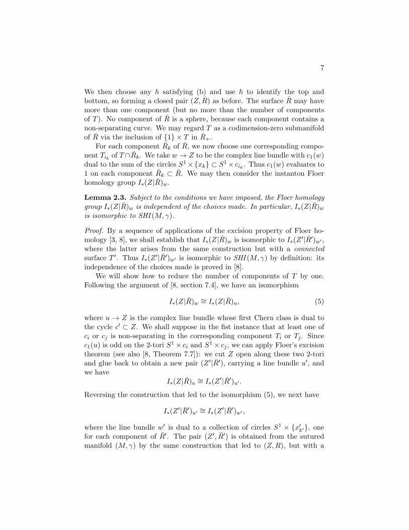
We then choose any h satisfying (b) and use h to identify the top andbottom, so forming a closed pair (Z, R) as before. The surface R may havemore than one component (but no more than the number of componentsof T ). No component of R is a sphere, because each component contains anon-separating curve. We may regard T as a codimension-zero submanifoldof R via the inclusion of {1} × T in R+.

For each component Rk of R, we now choose one corresponding compo-nent Tik of T ∩Rk. We take w → Z to be the complex line bundle with c1(w)dual to the sum of the circles S1×{xk} ⊂ S1× cik . Thus c1(w) evaluates to1 on each component Rk ⊂ R. We may then consider the instanton Floerhomology group I∗(Z|R)w.

Lemma 2.3. Subject to the conditions we have imposed, the Floer homologygroup I∗(Z|R)w is independent of the choices made. In particular, I∗(Z|R)wis isomorphic to SHI (M,γ).

Proof. By a sequence of applications of the excision property of Floer ho-mology [3, 8], we shall establish that I∗(Z|R)w is isomorphic to I∗(Z

′|R′)w′ ,where the latter arises from the same construction but with a connectedsurface T ′. Thus I∗(Z

′|R′)w′ is isomorphic to SHI (M,γ) by definition: itsindependence of the choices made is proved in [8].

We will show how to reduce the number of components of T by one.Following the argument of [8, section 7.4], we have an isomorphism

I∗(Z|R)w ∼= I∗(Z|R)u, (5)

where u → Z is the complex line bundle whose first Chern class is dual tothe cycle c′ ⊂ Z. We shall suppose in the fist instance that at least one ofci or cj is non-separating in the corresponding component Ti or Tj . Sincec1(u) is odd on the 2-tori S1× ci and S1× cj , we can apply Floer’s excisiontheorem (see also [8, Theorem 7.7]): we cut Z open along these two 2-toriand glue back to obtain a new pair (Z ′|R′), carrying a line bundle u′, andwe have

I∗(Z|R)u ∼= I∗(Z′|R′)u′ .

Reversing the construction that led to the isomorphism (5), we next have

I∗(Z′|R′)u′ ∼= I∗(Z

′|R′)w′ ,

where the line bundle w′ is dual to a collection of circles S1 × {x′k′}, onefor each component of R′. The pair (Z ′, R′) is obtained from the suturedmanifold (M,γ) by the same construction that led to (Z,R), but with a

8

surface T ′ having one fewer components: the components Ti and Tj havebeen joined into one component by cutting open along the circles ci and cjand reglueing.

If both ci and cj are separating in Ti and Tj respectively, then the aboveargument fails, because T ′ will have the same number of components asT . In this case, we can alter Ti and ci to make a new T ′i and c′i, with c′inon-separating in T ′i . For example, we may replace Z by the disjoint unionZ q Z∗, where Z∗ is a product S1 × T∗, with T∗ of genus 2. In the samemanner as above, we can cut Z along S1× ci and cut Z∗ along S1× c∗, andthen reglue, interchanging the boundary components. The effect of this isto replace Ti be a surface T ′i of genus one larger. We can take c′i to be anon-separating curve on T∗ \ c∗.

2.4 Instanton homology for knots and links

Consider a link K in a closed oriented 3-manifold Y . Following Juhasz [4],we can associate to (Y,K) a sutured manifold (M,γ) by taking M to be thelink complement and taking the sutures s(γ) to consist of two oppositely-oriented meridional curves on each of the tori in ∂M . As in [8], where thecase of knots was discussed, we take Juhasz’ prescription as a definition forthe instanton knot (or link) homology of the pair (Y,K):

Definition 2.4 (cf. [4]). We define the instanton homology of the linkK ⊂ Y to be the instanton Floer homology of the sutured manifold (M,γ)obtained from the link complement as above. Thus,

KHI (Y,K) = SHI (M,γ).

♦

Although we are free to choose any admissible closure Z in constructingSHI (M,γ), we can exploit the fact that we are dealing with a link comple-ment to narrow our choices. Let r be the number of components of the linkK. Orient K and choose a longitudinal oriented curve li ⊂ ∂M on the pe-ripheral torus of each component Ki ⊂ K. Let Fr be a genus-1 surface withr boundary components, δ1, . . . , δr. Form a closed manifold Z by attachingFr × S1 to M along their boundaries:

Z = (Y \No(K)) ∪ (Fr × S1). (6)

The attaching is done so that the curve pi×S1 for pi ∈ δi is attached to themeridian of Ki and δi × {q} is attached to the chosen longitude li. We can

9

view Z as a closure of (M,γ) in which the auxiliary surface T consists of rannuli,

T = T1 ∪ · · · ∪ Tr.

The two sutures of the product sutured manifold [−1, 1] × Ti are attachedto meridional sutures on the components of ∂M corresponding to Ki andKi−1 in some cyclic ordering of the components. Viewed this way, thecorresponding surface R ⊂ Z is the torus

R = ν × S1

where ν ⊂ Fr is a closed curve representing a generator of the homology ofthe closed genus-1 surface obtained by adding disks to Fr. Because R is atorus, the group I∗(Z|R)w can be more simply described as the generalizedeigenspace of µ(y) belonging to the eigenvalue 2, for which we temporarilyintroduce the notation I∗(Z)w,+2. Thus we can write

KHI (Y,K) = I∗(Z)w,+2.

An important special case for us is when K ⊂ Y is null-homologous inY with its given orientation. In this case, we may choose a Seifert surfaceΣ, which we regard as a properly embedded oriented surface in M withoriented boundary a union of longitudinal curves, one for each componentof K. When a Seifert surface is given, we have a uniquely preferred closureZ, obtained as above but using the longitudes provided by ∂Σ. Let us fixa Seifert surface Σ and write σ for its homology class in H2(M,∂M). Thepreferred closure of the sutured link complement is entirely determined byσ.

2.5 The decomposition into generalized eigenspaces

We continue to suppose that Σ is a Seifert surface for the null-homologousoriented knot K ⊂ Y . We write (M,γ) for the sutured link complement andZ for the preferred closure.

The homology class σ = [Σ] in H2(M,∂M) extends to a class σ = [Σ] inH2(Z): the surface Σ is formed from the Seifert surface Σ and Fr,

Σ = Σ ∪ Fr.

The homology class σ determines an endomorphism

µ(σ) : I∗(Z)w,+2 → I∗(Z)w,+2.

10

This endomorphism is traceless, a consequence of the relative Z/8 grading:there is an endomorphism ε of I∗(Z)w given by multiplication by (

√−1)s

on the part of relative grading s, and this ε commutes with µ(y) and anti-commutes with µ(σ). We write this traceless endomorphism as

µo(σ) ∈ sl(KHI (Y,K)). (7)

Our notation hides the fact that the construction depends (a priori) on theexistence of the preferred closure Z, so that KHI (Y,K) can be canonicallyidentified with I∗(Z)w,+2.

It now follows from [8, Proposition 7.5] that the eigenvalues of µo(σ) areeven integers 2j in the range −2g + 2 ≤ 2j ≤ 2g − 2, where g = g(Σ) + r isthe genus of Σ. Thus:

Definition 2.5. For a null-homologous oriented link K ⊂ Y with a chosenSeifert surface Σ, we write

KHI (Y,K, [Σ], j) ⊂ KHI (Y,K)

for the generalized eigenspace of µo([Σ]) belonging to the eigenvalue 2j, sothat

KHI (Y,K) =

g(Σ)−1+r⊕j=−g(Σ)+1−r

KHI (Y,K, [Σ], j),

where r is the number of components of K. If Y is a homology sphere,we may omit [Σ] from the notation; and if Y is S3 then we simply writeKHI (K, j). ♦

Remark. The authors believe that, for a general sutured manifold (M,γ),one can define a unique linear map

µo : H2(M,∂M)→ sl(SHI (M,γ))

characterized by the property that for any admissible closure (Z, R) and anyσ in H2(Z) extending σ ∈ H2(M,∂M) we have

µo(σ) = traceless part of µ(σ),

under a suitable identification of I∗(Z|R)w with SHI (M,γ). The authorswill return to this question in a future paper. For now, we are exploitingthe existence of a preferred closure Z so as to side-step the issue of whetherµo would be well-defined, independent of the choices made.

11

2.6 The mod 2 grading

If Y is a closed 3-manifold, then the instanton homology group I∗(Y )w hasa canonical decomposition into parts of even and odd grading mod 2. Forthe purposes of this paper, we normalize our conventions so that the twogenerators of I∗(T

3)w = C2 are in odd degree. As in [6, section 25.4 ], thecanonical mod 2 grading is then essentially determined by the property that,for a cobordism W from a manifold Y− to Y+, the induced map on Floerhomology has even or odd grading according to the parity of the integer

ι(W ) =1

2

(χ(W ) + σ(W ) + b1(Y+)− b0(Y+)− b1(Y−) + b0(Y−)

). (8)

(In the case of connected manifolds Y+ and Y−, this formula reduces to theone that appears in [6] for the monopole case. There is more than one wayto extend the formula to the case of disconnected manifolds, and we havesimply chosen one.) By declaring that the generators for T 3 are in odddegree, we ensure that the canonical mod 2 gradings behave as expectedfor disjoint unions of the 3-manifolds. Thus, if Y1 and Y2 are the connectedcomponents of a 3-manifold Y and α1⊗α2 is a class on Y obtained from αion Yi, then gr(α1 ⊗ α2) is gr(α1) + gr(α2) in Z/2 as expected.

Since the Floer homology SHI (M,γ) of a sutured manifold (M,γ) isdefined in terms of I∗(Z)w for an admissible closure Z, it is tempting totry to define a canonical mod 2 grading on SHI (M,γ) by carrying over thecanonical mod 2 grading from Z. This does not work, however, because theresult will depend on the choice of closure. This is illustrated by the factthat the mapping torus of a Dehn twist on T 2 may have Floer homology ineven degree in the canonical mod 2 grading (depending on the sign of theDehn twist), despite the fact that both T 3 and this mapping torus can beviewed as closures of the same sutured manifold.

We conclude from this that, without auxiliary choices, there is no canon-ical mod 2 grading on SHI (M,γ) in general: only a relative grading. Nev-ertheless, in the special case of an oriented null-homologous knot or link Kin a closed 3-manifold Y , we can fix a convention that gives an absolutemod 2 grading, once a Seifert surface Σ for K is given. We simply take thepreferred closure Z described above in section 2.4, using ∂Σ again to definethe longitudes, so that KHI (Y,K) is identified with I∗(Z)w,+2, and we usethe canonical mod 2 grading from the latter.

With this convention, the unknot U has KHI (U) of rank 1, with a singlegenerator in odd grading mod 2.

12

3 The skein sequence

3.1 The long exact sequence

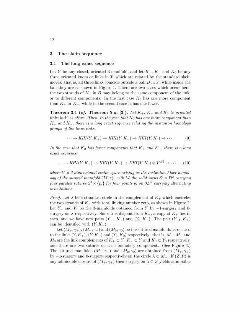
Let Y be any closed, oriented 3-manifold, and let K+, K− and K0 be anythree oriented knots or links in Y which are related by the standard skeinmoves: that is, all three links coincide outside a ball B in Y , while inside theball they are as shown in Figure 1. There are two cases which occur here:the two strands of K+ in B may belong to the same component of the link,or to different components. In the first case K0 has one more componentthan K+ or K−, while in the second case it has one fewer.

Theorem 3.1 (cf. Theorem 5 of [3]). Let K+, K− and K0 be orientedlinks in Y as above. Then, in the case that K0 has one more component thanK+ and K−, there is a long exact sequence relating the instanton homologygroups of the three links,

· · · → KHI (Y,K+)→ KHI (Y,K−)→ KHI (Y,K0)→ · · · . (9)

In the case that K0 has fewer components that K+ and K−, there is a longexact sequence

· · · → KHI (Y,K+)→ KHI (Y,K−)→ KHI (Y,K0)⊗ V ⊗2 → · · · (10)

where V a 2-dimensional vector space arising as the instanton Floer homol-ogy of the sutured manifold (M,γ), with M the solid torus S1×D2 carryingfour parallel sutures S1×{pi} for four points pi on ∂D2 carrying alternatingorientations.

Proof. Let λ be a standard circle in the complement of K+ which encirclesthe two strands of K+ with total linking number zero, as shown in Figure 2.Let Y− and Y0 be the 3-manifolds obtained from Y by −1-surgery and 0-surgery on λ respectively. Since λ is disjoint from K+, a copy of K+ lies ineach, and we have new pairs (Y−1,K+) and (Y0,K+). The pair (Y−1,K+)can be identified with (Y,K−).

Let (M+, γ+), (M−, γ−) and (M0, γ0) be the sutured manifolds associatedto the links (Y,K+), (Y,K−) and (Y0,K0) respectively: that is, M+, M− andM0 are the link complements of K+ ⊂ Y , K− ⊂ Y and K0 ⊂ Y0 respectively,and there are two sutures on each boundary component. (See Figure 3.)The sutured manifolds (M−, γ−) and (M0, γ0) are obtained from (M+, γ+)by −1-surgery and 0-surgery respectively on the circle λ ⊂M+. If (Z, R) isany admissible closure of (M+, γ+) then surgery on λ ⊂ Z yields admissible

13

Figure 2: The knot K+, with a standard circle λ around a crossing, with linkingnumber zero.

Figure 3: Sutured manifolds obtained from the knot complement, related by asurgery exact triangle.

14

Figure 4: Decomposing M0 along a product annulus to obtain a link complementin S3.

closures for the other two sutured manifolds. From Floer’s surgery exacttriangle [1], it follows that there is a long exact sequence

· · · → SHI (M+, γ+)→ SHI (M−, γ−)→ SHI (M0, γ0)→ · · · (11)

in which the maps are induced by surgery cobordisms between admissibleclosures of the sutured manifolds.

By definition, we have

SHI (M+, γ+) = KHI (Y,K+)

SHI (M−, γ−) = KHI (Y,K−).

However, the situation for (M0, γ0) is a little different. The manifold M0 isobtained by zero-surgery on the circle λ in M+, as indicated in Figure 3.This sutured manifold contains a product annulus S, consisting of the unionof the twice-punctured disk shown in Figure 4 and a disk D2 in the surgerysolid-torus S1×D2. As shown in the figure, sutured-manifold decompositionalong the annulus S gives a sutured manifold (M ′0, γ

′0) in which M ′0 is the

link complement of K0 ⊂ Y :

(M0, γ0)S (M ′0, γ

′0).

By Proposition 6.7 of [8] (as adapted to the instanton homology setting insection 7.5 of that paper), we therefore have an isomorphism

SHI (M0, γ0) ∼= SHI (M ′0, γ′0).

We now have to separate cases according to the number of componentsof K+ and K0. If the two strands of K+ at the crossing belong to the same

15

Figure 5: Removing some extra sutures using a decomposition along a productannulus. The solid torus in the last step has four sutures.

component, then every component of ∂M ′0 contains exactly two, oppositely-oriented sutures, and we therefore have

SHI (M ′0, γ′0) = KHI (Y,K0).

In this case, the sequence (11) becomes the sequence in the first case of thetheorem.

If the two strands of K+ belong to different components, then the corre-sponding boundary components of M+ each carry two sutures. These twoboundary components become one boundary component in M ′0, and the de-composition along S introduces two new sutures; so the resulting boundary

16

component in M ′0 carries six meridional sutures, with alternating orienta-tions. Thus (M ′0, γ

′0) fails to be the sutured manifold associated to the link

K0 ⊂ Y , on account of having four additional sutures. As shown in Figure 5however, the number of sutures on a torus boundary component can alwaysbe reduced by 2 (as long as there are at least four to start with) by usinga decomposition along a separating annulus. This decomposition results ina manifold with one additional connected component, which is a solid toruswith four longitudinal sutures. This operation needs to be performed twiceto reduce the number of sutures in M ′0 by four, so we obtain two copiesof this solid torus. Denoting by V the Floer homology of this four-suturedsolid-torus, we therefore have

SHI (M ′0, γ′0) = KHI (Y,K0)⊗ V ⊗ V

in this case. Thus the sequence (11) becomes the second long exact sequencein the theorem.

At this point, all that remains is to show that V is 2-dimensional, asasserted in the theorem. We will do this indirectly, by identifying V ⊗ V asa 4-dimensional vector space. Let (M4, γ4) be the sutured solid-torus with4 longitudinal sutures, as described above, so that SHI (M4, γ4) = V . Let(M,γ) be two disjoint copies of (M4, γ4), so that

SHI (M,γ) = V ⊗ V.

We can describe an admissible closure of (M,γ) (with a disconnected Tas in section 2.3) by taking T to be four annuli: we attach [−1, 1] × T to(M,γ) to form M so that M is Σ×S1 with Σ a four-punctured sphere. Thus∂M consists of four tori, two of which belong to R+ and two to R−. Theclosure (Y, R) is obtained by gluing the tori in pairs; and this can be doneso that Y has the form Σ2 × S1, where Σ2 is now a closed surface of genus2. The surface R in Σ2 × S1 has the form γ × S1, where γ is a union of twodisjoint closed curves in independent homology classes. The line bundle whas c1(w) dual to γ′, where γ′ is a curve on Σ2 dual to one component of γ.

Thus we can identify V ⊗ V with the generalized eigenspace of µ(y)belonging to the eigenvalue +2 in the Floer homology I∗(Σ2 × S1)w,

V ⊗ V = I∗(Σ2 × S1)w,+2, (12)

where w is dual to a curve lying on Σ2. Our next task is therefore to identifythis Floer homology group. This was done (in slightly different language) byBraam and Donaldson [1, Proposition 1.15]. The main point is to identifythe relevant representation variety in B(Y )w, for which we quote:

17

Lemma 3.2 ([1]). For Y = Σ2 × S1 and w as above, the critical-pointset of the Chern-Simons functional in B(Y )w consists of two disjoint 2-tori.Furthermore, the Chern-Simons functional is of Morse-Bott type along itscritical locus.

To continue the calculation, following [1], it now follows from the lemmathat I∗(Σ2×S1)w has dimension at most 8 and that the even and odd partsof this Floer group, with respect to the relative mod 2 grading, have equaldimension: each at most 4. On the other hand, the group I∗(Σ2 × S1|Σ2)wis non-zero. So the generalized eigenspaces belonging to the eigenvalue-pairs ((−1)r2, ir2), for r = 0, 1, 2, 3, are all non-zero. Indeed, each of thesegeneralized eigenspaces is 1-dimensional, by Proposition 7.9 of [8]. Thesefour 1-dimensional generalized eigenspaces all belong to the same relativemod-2 grading. It follows that I∗(Σ2 × S1)w is 8-dimensional, and can beidentified as a vector space with the homology of the critical-point set. Thegeneralized eigenspace belonging to +2 for the operator µ(y) is therefore4-dimensional; and this is V ⊗ V . This completes the argument.

3.2 Tracking the mod 2 grading

Because we wish to examine the Euler characteristics, we need to know howthe canonical mod 2 grading behaves under the maps in Theorem 3.1. Thisis the content of the next lemma.

Lemma 3.3. In the situation of Theorem 3.1, suppose that the link K+ isnull-homologous (so that K− and K0 are null-homologous also). Let Σ+ bea Seifert surface for K+, and let Σ− and Σ0 be Seifert surfaces for the othertwo links, obtained from Σ+ by a modification in the neighborhood of thecrossing. Equip the instanton knot homology groups of these links with theircanonical mod 2 gradings, as determined by the preferred closures arisingfrom these Seifert surfaces. Then in the first case of the two cases of thetheorem, the map from KHI (Y,K−) to KHI (Y,K0) in the sequence (9) hasodd degree, while the other two maps have even degree, with respect to thecanonical mod 2 grading.

In the second case, if we grade the 4-dimensional vector space V ⊗ Vby identifying it with I∗(Σ2 × S1)w,+2 as in (12), then the map fromKHI (Y,K0) ⊗ V ⊗2 to KHI (Y,K+) in (10) has odd degree, while the othertwo maps have even degree.

Proof. We begin with the first case. Let Z+ be the preferred closure of thesutured knot complement (M+, γ+) obtained from the knot K+, as defined

18

by (6). In the notation of the proof of Theorem 3.1, the curve λ lies in Z+.Let us write Z− and Z0 for the manifolds obtained from Z+ by −1-surgeryand 0-surgery on λ respectively. It is a straightforward observation that Z−and Z0 are respectively the preferred closures of the sutured complements ofthe links K− and K0. The surgery cobordism W from Z+ to Z− gives rise tothe map from KHI (Y,K+) to KHI (Y,K−). This W has the same homologyas the cylinder [−1, 1]× Z+ blown up at a single point. The quantity ι(W )in (8) is therefore even, and it follows that the map

KHI (Y,K+)→ KHI (Y,K−)

has even degree. The surgery cobordism W0 induces a map

I∗(Z−)w → I∗(Z0)w (13)

which has odd degree, by another application of (8). This concludes theproof of the first case.

In the second case of the theorem, we still have a long exact sequence

→ I∗(Z+)w → I∗(Z−)w → I∗(Z0)w →

in which the map I∗(Z−)w → I∗(Z0)w is odd and the other two are even.However, it is no longer true that the manifold Z0 is the preferred closure ofthe sutured manifold obtained from K0. The manifold Z0 can be describedas being obtained from the complement of K0 by attaching Gr × S1, whereGr is a surface of genus 2 with r boundary components. Here r is the numberof components of K0, and the attaching is done as before, so that the curves∂Gr×{q} is attached to the longitudes and the curves {pi}×S1 are attachedto the meridians. The preferred closure, on the other hand, is defined usinga surface Fr of genus 1, not genus 2. We write Z ′0 for the preferred closure,and our remaining task is to compare the instanton Floer homologies of Z0

and Z ′0, with their canonical Z/2 gradings.An application of Floer’s excision theorem provides an isomorphism

I∗(Z0)w,+2 → I∗(Z′0)w,+2 ⊗ I∗(Σ2 × S1)w,+2

where (as before) the class w in the last term is dual to a non-separatingcurve in the genus-2 surface Σ2. (See Figure 6 which depicts the excisioncobordism from Gr × S1 to (Fr qΣ2)× S1, with the S1 factor suppressed.)The isomorphism is realized by an explicit cobordism W , with ι(W ) odd,which accounts for the difference between the first and second cases andconcludes the proof.

19

Figure 6: The surfaces Gr and FrqΣ2, used in constructing Z0 and Z ′0 respectively.

3.3 Tracking the eigenspace decomposition

The next lemma is similar in spirit to Lemma 3.3, but deals with eigenspacedecomposition rather than the mod 2 grading.

Lemma 3.4. In the situation of Theorem 3.1, suppose again that the linksK+, K− and K0 are null-homologous. Let Σ+ be a Seifert surface for K+,and let Σ− and Σ0 be Seifert surfaces for the other two links, obtained fromΣ+ by a modification in the neighborhood of the crossing. Then in the firstcase of the two cases of the theorem, the maps in the long exact sequence (9)intertwine the three operators µo([Σ+]), µo([Σ−]) and µo([Σ0]). In particularthen, we have a long exact sequence

→ KHI (Y,K+, [Σ+], j)→ KHI (Y,K−, [Σ−], j)→ KHI (Y,K0, [Σ0], j)→

for every j.In the second case of Theorem 3.1, the maps in the long exact sequence

(10) intertwine the operators µo([Σ+]) and µo([Σ−]) on the first two termswith the operator

µo([Σ0])⊗ 1 + 1⊗ µ([Σ2])

acting on

KHI (Y,K0)⊗ I∗(Σ2 × S1)w,+2∼= KHI (Y,K0)⊗ V ⊗2.

Proof. The operator µo([Σ]) on the knot homology groups is defined in termsof the action of µ([Σ]) for a corresponding closed surface Σ in the preferredclosure of the link complement. The maps in the long exact sequences arisefrom cobordisms between the preferred closures. The lemma follows fromthe fact that the corresponding closed surfaces are homologous in thesecobordisms.

20

3.4 Proof of the main theorem

For a null-homologous link K ⊂ Y with a chosen Seifert surface Σ, let uswrite

χ(Y,K, [Σ]) =∑j

χ(KHI (Y,K, [Σ], j))tj

=∑j

(dim KHI 0(Y,K, [Σ], j)− dim KHI 1(Y,K, [Σ], j)

)tj

= str(tµo(Σ)/2),

where str denotes the alternating trace. If K+, K− and K0 are three skein-related links with corresponding Seifert surfaces Σ+, Σ− and Σ0, then The-orem 3.1, Lemma 3.3 and Lemma 3.4 together tell us that we have therelation

χ(Y,K+, [Σ+])− χ(Y,K−, [Σ−]) + χ(Y,K0, [Σ0]) = 0

in the first case of Theorem 3.1, and

χ(Y,K+, [Σ+])− χ(Y,K−, [Σ−])− χ(Y,K0, [Σ0])r(t) = 0

in the second case. Here r(t) is the contribution from the term I∗(Σ2 ×S1)w,+2, so that

r(t) = str(tµ([Σ2])/2).

From the proof of Lemma 3.2 we can read off the eigenvalues of [Σ2]/2: theyare 1, 0 and −1, and the ±1 eigenspaces are each 1-dimensional. Thus

r(t) = ±(t− 2 + t−1).

To determine the sign of r(t), we need to know the canonical Z/2 grad-ing of (say) the 0-eigenspace of µ([Σ2]) in I∗(Σ2 × S1)w,+2. The trivial3-dimensional cobordism from T 2 to T 2 can be decomposed as N+ ∪ N−,where N+ is a cobordism from T 2 to Σ2 and N− is a cobordism the otherway. The 4-dimensional cobordisms W± = N± × S1 induce isomorphismson the 0-eigenspace of µ([T 2]) = µ([Σ2]); and ι(W±) is odd. Since the gen-erator for T 3 is in odd degree, we conclude that the 0-eigenspace of µ([Σ2])is in even degree, and that

r(t) = −(t− 2 + t−1)

= −q(t)2

21

where

q(t) = (t1/2 − t−1/2).

We can roll the two case of Theorem 3.1 into one by defining the “nor-malized” Euler characteristic as

χ(Y,K, [Σ]) = q(t)1−rχ(Y,K, [Σ]) (14)

where r is the number of components of the link K. With this notation wehave:

Proposition 3.5. For null-homologous skein-related links K+, K− and K0

with corresponding Seifert surface Σ+, Σ− and Σ0, the normalized Eulercharacteristics (14) satisfy

χ(Y,K+, [Σ+])− χ(Y,K−, [Σ−]) = (t1/2 − t−1/2) χ(Y,K0, [Σ0]).

In the case of classical knots and links, we may write this simply as

χ(K+)− χ(K−) = (t1/2 − t−1/2) χ(K0).

This is the exactly the skein relation of the (single-variable) normalizedAlexander polynomial ∆. The latter is normalized so that ∆ = 1 for theunknot, whereas our χ is −1 for the unknot because the generator of itsknot homology is in odd degree. We therefore have:

Theorem 3.6. For any link K in S3, we have

χ(K) = −∆K(t),

where χ(K) is the normalized Euler characteristic (14) and ∆K is theAlexander polynomial of the link with Conway’s normalization.

In the case that K is a knot, we have χ(K) = χ(K), which is the casegiven in Theorem 1.1 in the introduction.

Remark. The equality r(t) = −q(t)2 can be interpreted as arising from theisomorphism

I∗(Σ2 × S1)w,+2∼= V ⊗ V,

with the additional observation that the isomorphism between these two isodd with respect to the preferred Z/2 gradings.

22

4 Applications

4.1 Fibered knots

In [8], the authors adapted the argument of Ni [11] to establish a criterionfor a knot K in S3 to be a fibered knot: in particular, Corollary 7.19 of [8]states that K is fibered if the following three conditions hold:

(a) the Alexander polynomial ∆K(T ) is monic, in the sense that its leadingcoefficient is ±1;

(b) the leading coefficient occurs in degree g, where g is the genus of theknot; and

(c) the dimension of KHI (K, g) is 1.

It follows from our Theorem 1.1 that the last of these three conditions impliesthe other two. So we have:

Proposition 4.1. If K is a knot in S3 of genus g, then K is fibered if andonly if the dimension of KHI (K, g) is 1.

4.2 Counting representations

We describe some applications to representation varieties associated to clas-sical knots K ⊂ S3. The instanton knot homology KHI (K) is defined interms of the preferred closure Z = Z(K) described at (6), and thereforeinvolves the flat connections

R(Z)w ⊂ B(Z)w

in the space of connections B(Z)w: the quotient by the determinant-1 gaugegroup of the space of all PU (2) connections in P(Ew), where Ew → Z isa U(2) bundle with det(E) = w. If the space of these flat connections inB(Z)w is non-degenerate in the Morse-Bott sense when regarded as the setof critical points of the Chern-Simons functional, then we have

dim I∗(Z)w ≤ dimH∗(R(Z)w).

The generalized eigenspace I∗(Z)w,+2 ⊂ I∗(Z)w has half the dimension ofthe total, so

dim KHI (K) ≤ 1

2dimH∗(R(Z)w).

23

As explained in [8], the representation variety R(Z)w is closely relatedto the space

R(K, i) = { ρ : π1(S3 \K)→ SU (2) | ρ(m) = i },

where m is a chosen meridian and

i =

(i 00 −i

).

More particularly, there is a two-to-one covering map

R(Z)w → R(K, i). (15)

The circle subgroup SU (2)i ⊂ SU (2) which stabilizes i acts on R(K, i) byconjugation. There is a unique reducible element inR(K, i) which is fixed bythe circle action; the remaining elements are irreducible and have stabilizer±1. The most non-degenerate situation that can arise, therefore, is thatR(K, i) consists of a point (the reducible) together with finitely many circles,each of which is Morse-Bott. In such a case, the covering (15) is trivial. Asin [7], the corresponding non-degeneracy condition at a flat connection ρcan be interpreted as the condition that the map

H1(S3 \K; gρ)→ H1(m; gρ) = R

is an isomorphism. Here gρ is the local system on the knot complement withfiber su(2), associated to the representation ρ. We therefore have:

Corollary 4.2. Suppose that the representation variety R(K, i) associatedto the complement of a classical knot K ⊂ S3 consists of the reducible rep-resentation and n(K) conjugacy classes of irreducibles, each of which isnon-degenerate in the above sense. Then

dim KHI (K) ≤ 1 + 2n(K).

Proof. Under the given hypotheses, the representation variety R(K, i) is aunion of a single point and n(K) circles. Its total Betti number is therefore1 + 2n(K). The representation variety R(Z)w is a trivial double cover (15),so the total Betti number of R(Z)w is twice as large, 2 + 4n(K).

Combining this with Corollary 1.2, we obtain:

24

Corollary 4.3. Under the hypotheses of the previous corollary, we have

d∑j=−d

|aj | ≤ 1 + 2n(K)

where the aj are the coefficients of the Alexander polynomial.

Among all the irreducible elements of R(K, i), we can distinguish thesubset consisting of those ρ whose image is binary dihedral: contained, thatis, in the normalizer of a circle subgroup whose infinitesimal generator Jsatisfies Ad(i)(J) = −J . If n′(K) denotes the number of such irreduciblebinary dihedral representations, then one has

|det(K)| = 1 + 2n′(K).

(see [5]). On the other hand, the determinant det(K) can also be computedas the value of the Alexander polynomial at −1: the alternating sum of thecoefficients. Thus we have:

Corollary 4.4. Suppose that the Alexander polynomial of K fails to bealternating, in the sense that∣∣∣∣∣∣

d∑j=−d

(−1)jaj

∣∣∣∣∣∣ <d∑

j=−d|aj |.

Then either R(K, i) contains some representations that are not binary dihe-dral, or some of the binary-dihedral representations are degenerate as pointsof this representation variety.

This last corollary is nicely illustrated by the torus knot T (4, 3). Thisknot is the first non-alternating knot in Rolfsen’s tables [14], where it appearsas 819. The Alexander polynomial of 819 is not alternating in the sense of thecorollary; and as the corollary suggests, the representation variety R(819; i)contains representations that are not binary dihedral. Indeed, there arerepresentations whose image is the binary octahedral group in SU (2).

References

[1] P. J. Braam and S. K. Donaldson. Floer’s work on instanton homology, knotsand surgery. In The Floer memorial volume, volume 133 of Progr. Math., pages195–256. Birkhauser, Basel, 1995.

25

[2] S. K. Donaldson. Floer homology groups in Yang-Mills theory, volume 147 ofCambridge Tracts in Mathematics. Cambridge University Press, Cambridge,2002. With the assistance of M. Furuta and D. Kotschick.

[3] A. Floer. Instanton homology, surgery, and knots. In Geometry of low-dimensional manifolds, 1 (Durham, 1989), volume 150 of London Math. Soc.Lecture Note Ser., pages 97–114. Cambridge Univ. Press, Cambridge, 1990.

[4] A. Juhasz. Holomorphic discs and sutured manifolds. Algebr. Geom. Topol.,6:1429–1457 (electronic), 2006.

[5] E. P. Klassen. Representations of knot groups in SU(2). Trans. Amer. Math.Soc., 326(2):795–828, 1991.

[6] P. B. Kronheimer and T. S. Mrowka. Monopoles and three-manifolds. NewMathematical Monographs. Cambridge University Press, Cambridge, 2007.

[7] P. B. Kronheimer and T. S. Mrowka. Knot homology groups from instantons.Preprint, 2008.

[8] P. B. Kronheimer and T. S. Mrowka. Knots, sutures and excision. Preprint,2008.

[9] Y. Lim. Instanton homology and the Alexander polynomial. Preprint, 2009.

[10] V. Munoz. Ring structure of the Floer cohomology of Σ × S1. Topology,38(3):517–528, 1999.

[11] Y. Ni. Knot Floer homology detects fibred knots. Invent. Math., 170(3):577–608, 2007.

[12] P. Ozsvath and Z. Szabo. Holomorphic disks and knot invariants. Adv. Math.,186(1):58–116, 2004.

[13] J. Rasmussen. Floer homology and knot complements. PhD thesis, HarvardUniversity, 2003.

[14] D. Rolfsen. Knots and links, volume 7 of Mathematics Lecture Series. Publishor Perish Inc., Houston, TX, 1990. Corrected reprint of the 1976 original.