Embed Size (px)
Citation preview
DOI: 10.1007/s00222-007-0075-9Invent. math. 170, 577–608 (2007)
Knot Floer homology detects fibred knots
Yi Ni�
Department of Mathematics, Princeton University, Princeton, New Jersey 08544, USA(e-mail: [email protected])
Oblatum 10-X-2006 & 16-VIII-2007Published online: 20 September 2007 – © Springer-Verlag 2007
Dedicated to Professor Boju Jiang on the occasion of his 70th birthday
Abstract. Ozsvath and Szabo conjectured that knot Floer homology detectsfibred knots in S3. We will prove this conjecture for null-homologous knotsin arbitrary closed 3-manifolds. Namely, if K is a knot in a closed 3-mani-fold Y , Y − K is irreducible, and HFK(Y, K ) is monic, then K is fibred. Theproof relies on previous works due to Gabai, Ozsvath–Szabo, Ghiggini andthe author. A corollary is that if a knot in S3 admits a lens space surgery,then the knot is fibred.
1 Introduction
Knot Floer homology was introduced independently by Ozsvath–Szabo [13]and by Rasmussen [19]. For any null-homologous knot K ⊂ Y 3 with Seifertsurface F, one can associate to it some abelian groups HFK(Y, K, [F], i)for i ∈ Z. The knot Floer homology
HFK(Y, K ) ∼=⊕
i∈ZHFK(Y, K, [F], i)
is a finitely generated abelian group.A lot of topological information of the knot are contained in knot Floer
homology, in particular in the topmost filtration level. For example, Ozsvathand Szabo proved that the topmost filtration level of HFK for a knot in S3
is exactly the genus of the knot (see [14]).
� Current address: Department of Mathematics, Columbia University, Room 516, MC4406, 2990 Broadway, New York, NY 10027, USA
Mathematics Subject Classification (2000): 57R58, 57M27, 57R30
578 Y. Ni
When K is a fibred knot, it is shown that the topmost group of HFK(Y, K )is a single Z [16]. Ozsvath and Szabo conjectured that the converse is alsotrue for knots in S3 [18].
In this paper, we are going to prove this conjecture. Our main theorem is:
Theorem 1.1 Suppose K is a null-homologous knot in a closed, oriented,connected 3-manifold Y , Y − K is irreducible, and F is a genus-g Seifertsurface of K. If HFK(Y, K, [F], g) ∼= Z, then K is fibred, and F is a fibreof the fibration.
An oriented link L in Y is called a fibred link, if Y − L fibres over the circle,and L is the oriented boundary of the fibre. We have the following corollaryof Theorem 1.1:
Corollary 1.2 Suppose Y is a closed, oriented, connected 3-manifold, L isa null-homologous oriented link in Y , Y −L is irreducible, and F is a Seifertsurface of L. If HFK
(
Y, L,|L|−χ(F)
2
) ∼= Z, then L is a fibred link, and F isa fibre of the fibration.
The proof of this corollary will be given in Sect. 7.A rational homology sphere Y is called an L-space, if the rank of HF(Y )
is equal to | H1(Y ;Z)|. Many 3-manifolds are L-spaces, for example, themanifolds which admit spherical structures are L-spaces. An immediatecorollary of Theorem 1.1 is:
Corollary 1.3 If a knot K ⊂ S3 admits an L-space surgery, then K isa fibred knot. In particular, any knot that admits a lens space surgery isfibred.
Proof As a corollary of [17, Proposition 9.5], if a rational surgery on Kyields an L-space, then K also admits an L-space surgery with integercoefficient. Using [15, Theorem 1.2], we conclude that HFK(K, g) ∼= Z.Thus the desired result follows from Theorem 1.1. ��Corollary 1.4 Suppose Y is an L-space, K ⊂ Y is a null-homologousknot with genus g > 1. If the 0-surgery on K is a surface bundle over S1,then K is fibred.
Proof With the above conditions, one can prove that
HF+(Y0(K ), [g − 1]) ∼= HFK(Y, K, g).
In fact, the proof is exactly the same as the proof of [13, Corollary 4.5],so we will not give the details. The reader should note that, since Y isan L-space, HF+(Y ) is isomorphic to the direct sum of some copies ofZ[U, U−1]/UZ[U], hence the map ψ as in the proof of [13, Corollary 4.5]is surjective. Thus the argument there can be used.
Knot Floer homology detects fibred knots 579
Now since Y0(K ) fibres over the circle, we have HF+(Y0(K ), [g − 1])∼= Z, so HFK(Y, K, g) ∼= Z. It is easy to show that Y − K is irreducible,hence K is fibred by Theorem 1.1. ��Remark 1.5 The homology class [F] defines a homomorphism
f : π1(Y − K ) → Z
by counting the intersection numbers of [F] with loops. The famousStallings’ Fibration Theorem [20] says that K is a fibred knot with fibre inthe homology class of [F] if and only if ker f is finitely generated. HenceTheorem 1.1 indicates a mysterious relationship between Heegaard Floerhomology and the fundamental group.
Theorem 1.1 was previously examined in various sporadic cases, andsome theoretical evidences were given in [12], but the first real progresswas made by Ghiggini in [5], where a strategy to approach this conjecturewas proposed, and the special case of genus-one knots in S3 was proved.Ghiggini’s strategy plays an essential role in the present paper, we willapply this strategy by using a method introduced by Gabai [4]. Another keyingredient of this paper is the study of decomposition formulas for knotFloer homology, which is based on [12].
The paper is organized as follows. In Sect. 2, we give some backgroundson sutured manifolds. We will introduce a sutured manifold invariant whichnaturally comes from knot Floer homology. We also present a construction ofcertain Heegaard diagrams. In Sect. 3, we prove a homological version of themain theorem. Section 4 is devoted to prove the horizontal decompositionformula for knot Floer homology. In Sect. 5, we will prove a major technicaltheorem: the decomposition formula for knot Floer homology, in the caseof decomposing along a separating product annulus. In Sect. 6, we useGabai’s method to study Ghiggini’s strategy. As a result, we get a clearerpicture of the sutured manifold structure of the knot complement, namely,Theorem 6.2. Section 7 contains the proof of the main theorem, we use thedecomposition formulas we proved (especially Theorem 5.1) to reduce theproblem to the case that we already know.
Acknowledgements. This paper has been submitted to Princeton University as the author’sPhD thesis. We wish to thank David Gabai and Zoltan Szabo for their guidance.
We would like to thank Paolo Ghiggini for many fruitful discussions during the courseof this work. This paper benefits a lot from his work [5].
A version of Theorem 6.2 was also proved by Ian Agol via a different approach. Wewish to thank him for some interesting discussions.
We are grateful to Matthew Hedden, Andras Juhasz, Tao Li, Peter Ozsvath, Jiajun Wangand Chenyang Xu for some helpful conversations and their interests in this work. We areparticularly grateful to an anonymous referee for enormous suggestions and corrections.
The author was partially supported by a Graduate School Centennial Fellowship atPrinceton University. Parts of the work were carried out when the author visited UQAM andPeking University; he wishes to thank Steve Boyer, Olivier Collin and Shicheng Wang fortheir hospitality. The author extends his gratitude to the American Institute of Mathematicsand the Clay Mathematics Institute for their subsequent support.
580 Y. Ni
2 Preliminaries
2.1 Sutured manifold decomposition The theory of sutured manifolddecomposition was introduced by Gabai in [2]. We will briefly reviewthe basic definitions.
Definition 2.1 A sutured manifold (M, γ) is a compact oriented 3-mani-fold M together with a set γ ⊂ ∂M of pairwise disjoint annuli A(γ) andtori T(γ). The core of each component of A(γ) is a suture, and the set ofsutures is denoted by s(γ).
Every component of R(γ) = ∂M − int(γ) is oriented. Define R+(γ)(or R−(γ)) to be the union of those components of R(γ) whose normalvectors point out of (or into) M. The orientations on R(γ) must be co-herent with respect to s(γ), hence every component of A(γ) lies betweena component of R+(γ) and a component of R−(γ).
Definition 2.2 [11, Definition 2.2] A balanced sutured manifold is a suturedmanifold (M, γ) satisfying
(1) M has no closed components.(2) Every component of ∂M intersects γ nontrivially.(3) χ(R+(γ)) = χ(R−(γ)).
Definition 2.3 Let S be a compact oriented surface with connected compo-nents S1, . . . , Sn. We define
x(S) =∑
i
max{0,−χ(Si)}.
Let M be a compact oriented 3-manifold, A be a compact codimension-0submanifold of ∂M. Let h ∈ H2(M, A). The Thurston norm x(h) of h isdefined to be the minimal value of x(S), where S runs over all the properlyembedded surfaces in M with ∂S ⊂ A and [S] = h.
Definition 2.4 A sutured manifold (M, γ) is taut, if M is irreducible, andR(γ) is Thurston norm minimizing in H2(M, γ).
Definition 2.5 Let (M, γ) be a sutured manifold, and S a properly embeddedsurface in M, such that no component of ∂S bounds a disk in R(γ) and nocomponent of S is a disk with boundary in R(γ). Suppose that for everycomponent λ of S ∩ γ , one of (1)–(3) holds:
(1) λ is a properly embedded non-separating arc in γ .(2) λ is a simple closed curve in an annular component A of γ in the same
homology class as A ∩ s(γ).(3) λ is a homotopically nontrivial curve in a toral component T of γ , and
if δ is another component of T ∩ S, then λ and δ represent the samehomology class in H1(T ).
Knot Floer homology detects fibred knots 581
Then S is called a decomposition surface, and S defines a sutured manifolddecomposition
(M, γ)S� (M′, γ ′),
where M′ = M − int(Nd(S)) and
γ ′ = (γ ∩ M′) ∪ Nd(S′+ ∩ R−(γ)) ∪ Nd(S′
− ∩ R+(γ)),
R+(γ ′) = ((R+(γ) ∩ M′) ∪ S′+) − int(γ ′),
R−(γ ′) = ((R−(γ) ∩ M′) ∪ S′−) − int(γ ′),
where S′+ (S′−) is that component of ∂Nd(S) ∩ M′ whose normal vectorpoints out of (into) M′.
Definition 2.6 A decomposition surface is called a product disk, if it isa disk which intersects s(γ) in exactly two points. A decomposition surfaceis called a product annulus, if it is an annulus with one boundary componentin R+(γ), and the other boundary component in R−(γ).
Definition 2.7 A decomposition surface S in a balanced sutured manifoldis called a horizontal surface, if S has no closed component, |∂S| = |s(γ)|,[S] = [R+(γ)] ∈ H2(M, γ), and χ(S) = χ(R+).
Definition 2.8 A balanced sutured manifold (M, γ) is vertically prime, ifany horizontal surface S ⊂ M is parallel to either R−(γ) or R+(γ).
2.2 Knot Floer homology and an invariant of sutured manifolds Hee-gaard Floer homology has been proved to have very close relationship withThurston norm [14]. The definition of Thurston norm is purely topological(or combinatorial) [21], while the definition of Heegaard Floer homologyinvolves symplectic geometry and analysis. The bridge that connects thesetwo seemingly different topics is taut foliation.
The fundamental method of constructing taut foliations is sutured mani-fold decomposition [2]. Thus we naturally expect that, by studying the be-havior of Heegaard Floer homology under sutured manifold decomposition,we can get better understanding of the relationship between Heegaard Floerhomology and Thurston norm.
The first approach in such direction was taken in [12], where the “suturedHeegaard diagrams” for knots are introduced. Using them, one can studya very special case of sutured manifold decomposition: the Murasugi sum.Later on, Juhasz introduced an invariant for sutured manifolds, called“sutured Floer homology”, and proved some properties [11].
In this subsection, we will introduce another invariant of sutured mani-folds, which naturally comes from knot Floer homology. We will provesome decomposition formulas for this invariant in Sects. 4 and 5.
582 Y. Ni
Suppose L ⊂ Y is a null-homologous oriented link, F is a Seifertsurface of L . Decompose Y − int(Nd(L)) along F, we get a balancedsutured manifold (M, γ). The argument in [12, Proposition 3.5] shows that,if we cut open Y along F, reglue by a homeomorphism of F which is theidentity on the boundary, to get a new link L ′ in a new manifold Y ′, then
HFK
(
Y, L,|∂F| − χ(F)
2
)
∼= HFK
(
Y ′, L ′,|∂F| − χ(F)
2
)
as abelian groups. Therefore, HFK(
Y, L,|∂F|−χ(F)
2
)
can be viewed as aninvariant for the sutured manifold (M, γ). (For simplicity, let i(F) denote|∂F|−χ(F)
2 .)More precisely, suppose (M, γ) is a balanced sutured manifold, R±(γ)
are connected surfaces. There exists a diffeomorphism
ψ : R+(γ) → R−(γ),
such that for each component A of γ , ψ maps one boundary componentof A onto the other boundary component. We glue R+(γ) to R−(γ) by ψ,thus get a manifold with boundary consisting of tori. We fill each boundarytorus by a solid torus whose meridian intersects s(γ) exactly once. Nowwe get a closed 3-manifold Y . Let L be the union of the cores of the solidtori. The pair (Y, L) is denoted by ι(M, γ). Of course, ι(M, γ) depends onthe way we glue R+ to R− and the way we fill in the solid tori. In ourcase, changing the filling is equivalent to changing the gluing map by Dehntwists along the components of ∂R+. By the remark in the last paragraph,the abelian group
HFK(ι(M, γ), i(R+(γ)))
is independent of the choice of the gluing, hence it is independent of thechoice of ι(M, γ).
Proposition 2.9 There is a well-defined invariant HFS for balanced suturedmanifolds, which is characterized by the following two properties.
(1) If (M, γ) is a balanced sutured manifold, R±(γ) are connected, then
HFS(M, γ) ∼= HFK(ι(M, γ), i(R+(γ))).
(2) If
(M, γ)a×I� (M′, γ ′),
is the decomposition along a product disk then
HFS(M, γ) ∼= HFS(M′, γ ′).
Knot Floer homology detects fibred knots 583
Proof The inverse operation of the decomposition along a product disk, is“adding a product 1-handle” with feet at the suture. We first claim that, if(M, γ) is a balanced sutured manifold with R±(γ) connected, and (M1, γ1)is obtained by adding a product 1-handle to (M, γ), then
HFK(ι(M, γ), i(R+(γ))) ∼= HFK(ι(M1, γ1), i(R+(γ1))).
In fact, one possible choice of ι(M1, γ1) can be gotten by plumbing ι(M, γ)with (S2 × S1,Π). Here Π is a link in S2 × S1 which consists of twocopies of point × S1, but with different orientations. Now we can apply[12, Lemma 4.4] to get the claim.
Given a balanced sutured manifold (M, γ), we can add to it some product1-handles with feet at the suture to get a new balanced sutured manifold(M1, γ1), such that R±(γ1) are connected. We then define
HFS(M, γ) = HFK(ι(M1, γ1), i(R+(γ1))).
Now we want to prove that HFS(M, γ) is independent of the choice of(M1, γ1). For this purpose, let (M2 , γ2) be another sutured manifold obtainedby adding product 1-handles to (M, γ), and R±(γ2) are connected. We canassume that the feet of the product 1-handles for (M1, γ1) and (M2, γ2) aremutually different. Let (M3, γ3) be the sutured manifold obtained by addingall these product 1-handles (either for M1 or for M2) to (M, γ). By the claimproved in the first paragraph, we have
HFK(ι(M3, γ3), i(R+(γ3))) ∼= HFK(ι(M1, γ1), i(R+(γ1))),
HFK(ι(M3, γ3), i(R+(γ3))) ∼= HFK(ι(M2, γ2), i(R+(γ2))).
Therefore, HFS(M, γ) is well-defined.Property (1) holds by definition, and Property (2) can be proved by the
same argument as above. ��
2.3 Relative Morse functions and sutured diagrams Suppose K is a null-homologous knot in Y , F is a Seifert surface for K . In [12], the notion of“sutured Heegaard diagrams” was introduced. Such diagrams are useful tocompute HFK(Y, K, [F], g). A construction of sutured Heegaard diagramswas given in the proof of [12, Theorem 2.1].
In this subsection, we will present a slightly different construction, whichis based on relative Morse functions. This construction will be useful later.
Definition 2.10 [12, Definition 2.2] A double pointed Heegaard diagram
(Σ,α,β0 ∪ {µ}, w, z)
for (Y, K ) is a sutured Heegaard diagram, if it satisfies:
584 Y. Ni
(Su0) There exists a subsurface P ⊂ Σ, bounded by two curves α1 ∈ αand λ. g denotes the genus of P .
(Su1) λ is disjoint from β0. µ does not intersect any α curves except α1.µ intersects λ transversely in exactly one point, and intersects α1transversely in exactly one point. w, z ∈ λ lie in a small neighborhoodof λ∩µ, and on different sides of µ. (In practice, we often push w, zoff λ into P or Σ − P .)
(Su2) (α − {α1}) ∩ P consists of 2g arcs, which are linearly independentin H1(P , ∂P ). Moreover, Σ − α − P is connected.
Construction 2.11 Suppose (M, γ) is the sutured manifold obtained by cut-ting Y − int(Nd(K )) open along F. Let ψ : R+(γ) → R−(γ) be the gluingmap. Namely, if we glue R+(γ) to R−(γ) by ψ, then we get back themanifold Y − int(Nd(K )). We will construct a Heegaard diagram for thepair (Y, K ). The construction consists of 4 steps.
Step 0 A relative Morse function.
Consider a self-indexed relative Morse function u on (M, γ). Namely,u satisfies:
(1) u(M) = [0, 3], u−1(0) = R−(γ), u−1(3) = R+(γ).(2) u has no degenerate critical points. u is the standard height function
near γ . u−1{critical points of index i} = i.(3) u has no critical points on R(γ).
Let ˜F = u−1(
32
)
. ∂ ˜F is denoted by ˜λ. Similarly, the boundary componentsof R±(γ) are denoted by λ±.
Suppose u has r index-1 critical points, then the genus of ˜F is g + r.The gradient −∇u generates a flow φt on M. There are 2r points on R+(γ),which are connected to index-2 critical points by flowlines. We call thesepoints “bad” points. Similarly, there are 2r bad points on R−(γ), which areconnected to index-1 critical points by flowlines.
Step 1 Construct the curves.
Choose a small disk D+ in a neighborhood of λ+ in R+(γ). Choose an arcδ+ ⊂ R+(γ) connecting D+ to λ+. Flow D+ and δ+ by φt , their images on ˜Fand R−(γ) are ˜D, D−,˜δ, δ−. (Of course, we choose D+ and δ+ generically,so that the flowlines starting from them do not terminate at critical points.)We can suppose the gluing map ψ maps δ+ onto δ−, D+ onto D−. LetA± = R±(γ) − int(D±), ˜A = ˜F − int(˜D).
On ˜F, there are r simple closed curves α2g+2, . . . , α2g+1+r , which areconnected to index-1 critical points by flowlines. And there are r simpleclosed curves ˜β2g+2, . . . , ˜β2g+1+r , which are connected to index-2 criticalpoints by flowlines.
Choose 2g disjoint arcs ξ−2 , . . . , ξ−
2g+1 ⊂ A−, such that their endpointslie on λ−, and they are linearly independent in H1(A−, ∂A−). We also
Knot Floer homology detects fibred knots 585
suppose they are disjoint from δ− and the bad points. Let ξ+i = ψ−1(ξ−
i ).We also flow back ξ−
2 , . . . , ξ−2g+1 by φ−t to ˜F, the images are denoted
by ˜ξ2, . . . , ˜ξ2g+1.Choose 2g disjoint arcs η+
2 , . . . , η+2g+1 ⊂ A+, such that their endpoints
lie on ∂D+, and they are linearly independent in H1(A+, ∂A+). We alsosuppose they are disjoint from δ+ and the bad points. Flow them by φt to ˜F,the images are denoted by η2, . . . , η2g+1.
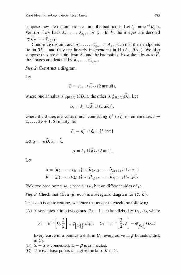
Step 2 Construct a diagram.
Let
Σ = A+ ∪ ˜A ∪ {2 annuli},where one annulus is φ[0,3/2](∂D+), the other is φ[0,3/2](˜λ). Let
αi = ξ+i ∪ ˜ξ i ∪ {2 arcs},
where the 2 arcs are vertical arcs connecting ξ+i to ˜ξ i on an annulus, i =
2, . . . , 2g + 1. Similarly, let
βi = η+i ∪ ηi ∪ {2 arcs}.
Let α1 = ∂ ˜D, λ = ˜λ,
µ = δ+ ∪˜δ ∪ {2 arcs}.Let
α = {α2, . . . , α2g+1} ∪ {α2g+2, . . . , α2g+1+r} ∪ {α1},β = {β2, . . . , β2g+1} ∪ {˜β2g+2, . . . , ˜β2g+1+r} ∪ {µ}.
Pick two base points w, z near λ ∩ µ, but on different sides of µ.
Step 3 Check that (Σ,α,β, w, z) is a Heegaard diagram for (Y, K ).
This step is quite routine, we leave the reader to check the following
(A) Σ separates Y into two genus-(2g +1+ r) handlebodies U1, U2, where
U1 = u−1
[
0,3
2
]
∪ φ[
0, 32
](D+), U2 = u−1
[
3
2, 3
]
− φ[
0, 32
](D+).
Every curve in α bounds a disk in U1, every curve in β bounds a diskin U2.
(B) Σ − α is connected, Σ − β is connected.(C) The two base points w, z give the knot K in Y .
586 Y. Ni
Then
(Σ,α,β, w, z)
is a Heegaard diagram for (Y, K ). It is not hard to see that this is a suturedHeegaard diagram. ��
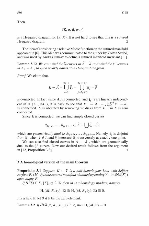
The idea of considering a relative Morse function on the sutured manifoldappeared in [6]. This idea was communicated to the author by Zoltan Szabo,and was used by Andras Juhasz to define a sutured manifold invariant [11].
Lemma 2.12 We can wind the α-curves in ˜A −˜δ, and wind the ξ+-curvesin A+ − δ+, to get a weakly admissible Heegaard diagram.
Proof We claim that,
E = ˜A −2g+1⋃
i=2
˜ξ i −2g+1+r⋃
j=2g+2
αj −˜δ
is connected. In fact, since A− is connected, and ξ−j ’s are linearly independ-
ent in H1(A−, ∂A−), it is easy to see that E− = A− − ⋃2g+1i=2 ξ−
i − δ−is connected. E is obtained by removing 2r disks from E−, so E is alsoconnected.
Since E is connected, we can find simple closed curves
θ2g+2, . . . , θ2g+1+r ⊂ ˜A −⋃
˜ξ i −˜δ,
which are geometrically dual to α2g+2, . . . , α2g+1+r . Namely, θj is disjointfrom αi when j �= i, and θi intersects αi transversely at exactly one point.
We can also find closed curves in A+ − δ+, which are geometricallydual to the ξ+-curves. Now our desired result follows from the argumentin [12, Proposition 3.3]. ��
3 A homological version of the main theorem
Proposition 3.1 Suppose K ⊂ Y is a null-homologous knot with Seifertsurface F, (M, γ) is the sutured manifold obtained by cutting Y−int(Nd(K ))open along F.
If HFK(Y, K, [F], g) ∼= Z, then M is a homology product, namely,
H∗(M, R−(γ);Z) ∼= H∗(M, R+(γ);Z) ∼= 0.
Fix a field F, let 0 ∈ F be the zero element.
Lemma 3.2 If HFK(Y, K, [F], g) ∼= Z, then H2(M;F) = 0.
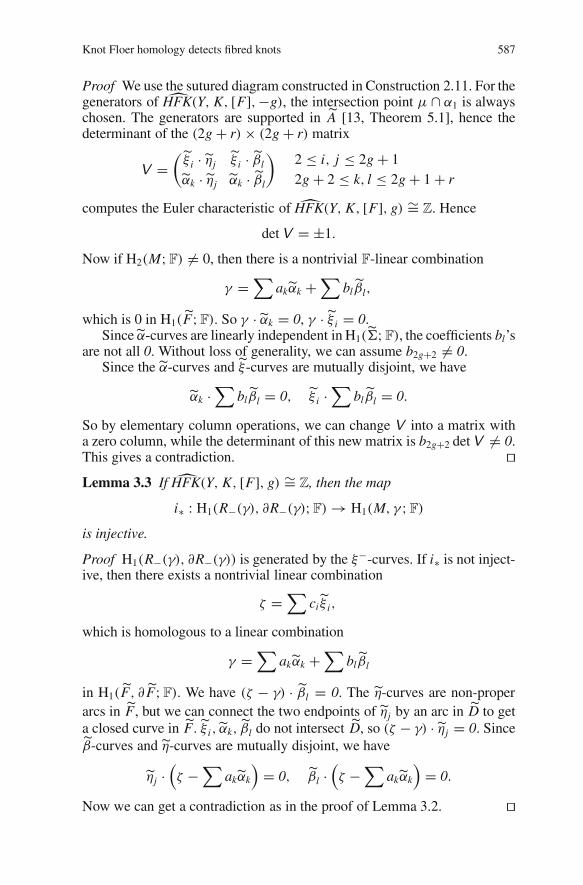
Knot Floer homology detects fibred knots 587
Proof We use the sutured diagram constructed in Construction 2.11. For thegenerators of HFK(Y, K, [F],−g), the intersection point µ ∩ α1 is alwayschosen. The generators are supported in ˜A [13, Theorem 5.1], hence thedeterminant of the (2g + r) × (2g + r) matrix
V =(
˜ξ i · ηj˜ξ i · ˜βl
αk · ηj αk · ˜βl
)
2 ≤ i, j ≤ 2g + 12g + 2 ≤ k, l ≤ 2g + 1 + r
computes the Euler characteristic of HFK(Y, K, [F], g) ∼= Z. Hence
detV = ±1.
Now if H2(M;F) �= 0, then there is a nontrivial F-linear combination
γ =∑
akαk +∑
bl˜βl,
which is 0 in H1(˜F;F). So γ · αk = 0, γ · ˜ξ i = 0.Since α-curves are linearly independent in H1(˜Σ;F), the coefficients bl’s
are not all 0. Without loss of generality, we can assume b2g+2 �= 0.Since the α-curves and ˜ξ-curves are mutually disjoint, we have
αk ·∑
bl˜βl = 0, ˜ξ i ·∑
bl˜βl = 0.
So by elementary column operations, we can change V into a matrix witha zero column, while the determinant of this new matrix is b2g+2 detV �= 0.This gives a contradiction. ��Lemma 3.3 If HFK(Y, K, [F], g) ∼= Z, then the map
i∗ : H1(R−(γ), ∂R−(γ);F) → H1(M, γ ;F)is injective.
Proof H1(R−(γ), ∂R−(γ)) is generated by the ξ−-curves. If i∗ is not inject-ive, then there exists a nontrivial linear combination
ζ =∑
ci˜ξ i,
which is homologous to a linear combination
γ =∑
akαk +∑
bl˜βl
in H1(˜F, ∂ ˜F;F). We have (ζ − γ) · ˜βl = 0. The η-curves are non-properarcs in ˜F, but we can connect the two endpoints of ηj by an arc in ˜D to geta closed curve in ˜F. ˜ξ i, αk, ˜βl do not intersect ˜D, so (ζ − γ) · ηj = 0. Since˜β-curves and η-curves are mutually disjoint, we have
ηj ·(
ζ −∑
akαk
)
= 0, ˜βl ·(
ζ −∑
akαk
)
= 0.
Now we can get a contradiction as in the proof of Lemma 3.2. ��
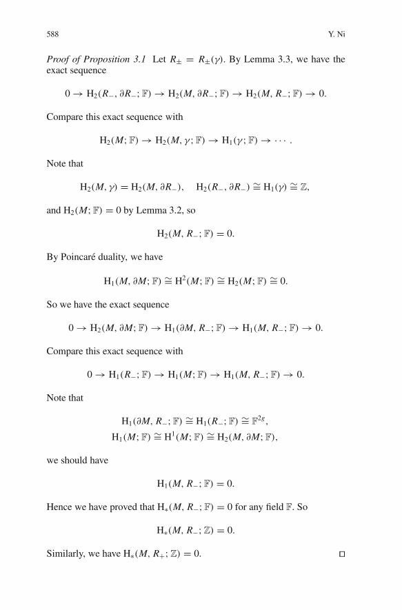
588 Y. Ni
Proof of Proposition 3.1 Let R± = R±(γ). By Lemma 3.3, we have theexact sequence
0 → H2(R−, ∂R−;F) → H2(M, ∂R−;F) → H2(M, R−;F) → 0.
Compare this exact sequence with
H2(M;F) → H2(M, γ ;F) → H1(γ ;F) → · · · .
Note that
H2(M, γ) = H2(M, ∂R−), H2(R−, ∂R−) ∼= H1(γ) ∼= Z,
and H2(M;F) = 0 by Lemma 3.2, so
H2(M, R−;F) = 0.
By Poincare duality, we have
H1(M, ∂M;F) ∼= H2(M;F) ∼= H2(M;F) ∼= 0.
So we have the exact sequence
0 → H2(M, ∂M;F) → H1(∂M, R−;F) → H1(M, R−;F) → 0.
Compare this exact sequence with
0 → H1(R−;F) → H1(M;F) → H1(M, R−;F) → 0.
Note that
H1(∂M, R−;F) ∼= H1(R−;F) ∼= F2g,
H1(M;F) ∼= H1(M;F) ∼= H2(M, ∂M;F),
we should have
H1(M, R−;F) = 0.
Hence we have proved that H∗(M, R−;F) = 0 for any field F. So
H∗(M, R−;Z) = 0.
Similarly, we have H∗(M, R+;Z) = 0. ��
Knot Floer homology detects fibred knots 589
4 Horizontal decomposition
Theorem 4.1 Let K ′ ⊂ Y ′, K ′′ ⊂ Y ′′ be two null-homologous knots. Sup-pose F ′, F ′′ are two genus-g Seifert surfaces for K ′, K ′′, respectively. Weconstruct a new manifold Y and a knot K ⊂ Y as follows. Cut open Y ′, Y ′′along F ′, F ′′, we get sutured manifolds (M′ , γ ′), (M′′, γ ′′). Now glue R+(γ ′)to R−(γ ′′), glue R+(γ ′′) to R−(γ ′), by two diffeomorphisms. We get a mani-fold Z with torus boundary. There is a simple closed curve µ ⊂ ∂Z, whichis the union of the two cut-open meridians of K ′, K ′′. We do Dehn fillingalong µ to get the manifold Y , the knot K is the core of the filled-in solidtorus.
Our conclusion is
HFK(Y, K, [F ′], g) ∼= HFK(Y ′, K ′, [F ′], g) ⊗ HFK(Y ′′, K ′′, [F ′′], g),
as linear spaces over any field F.
Remark 4.2 We did not specify the gluings, since they will not affect ourresult, thanks to [12, Proposition 3.5].
Remark 4.3 We clarify some convention we are going to use throughout thispaper. A holomorphic disk in the symmetric product is seen as an immersedsubsurface of the Heegaard surface Σ. Suppose Q is a subsurface of Σ, D1,. . . , Dn are the closures of the components of Q − ⋃
αi − ⋃
βj , choosea point zk in the interior of Dk for each k. If Φ is a holomorphic disk, thenΦ ∩ Q denotes the immersed surface
∑
k nzk(Φ)Dk.
Proof of Theorem 4.1 The proof uses the techniques from [12]. We constructa sutured Heegaard diagram (Σ′,α′,β′, w′, z′) for (Y ′, K ′), as in the proofof [12, Theorem 2.1]. The reader may refer to Fig. 1 there for a partialpicture.
As a result, Σ′ is the union of two compact surfaces A′, B′, where A′ isa genus g surface with two boundary components α′
1A, λ′A, and B′ is a genus
g + r ′ surface with two boundary components α′1B, λ′
B. A′ and B′ are gluedtogether, so that α′
1A and α′1B become one curve α′
1, λ′A and λ′
B become onecurve λ′.
We have
α′ = {α′1, α
′2, . . . , α
′2g+1, α
′2g+2, . . . , α
′2g+1+r′ },
β′ = {µ′, β′2, β
′3, . . . , β
′2g+1+r′ }.
Here α′i is the union of two arcs ξ ′
i ⊂ A′, ξ ′i ⊂ B′, for i = 2, . . . , 2g + 1.
α′j lie in B′, for j = 2g + 2, . . . , 2g + 1 + r ′. µ′ is the union of two arcs
δ′ ⊂ A′, δ′ ⊂ B′. µ′ intersects α′1 transversely in one point, and is disjoint
from all other α′-curves. β′i’s are disjoint from λ′.
Similarly, we construct a sutured diagram (Σ′′,α′′,β′′, w′′, z′′). Σ′′ is theunion of A′′, B′′. And the corresponding curves are denoted by α′′
i , β′′i , . . . .
590 Y. Ni
Now we glue A′, B′, A′′, B′′ together, so that α′1A and α′
1B become onecurve γ ′
1, λ′B and λ′′
A become one curve λ′, α′′1A and α′′
1B become one curve γ ′′1 ,
λ′′B and λ′
A become one curve λ′′. ξ ′i and ξ ′′
i are glued together to be a curve γ ′i ,
ξ ′′i and ξ ′
i are glued together to be a curve γ ′′i , i = 2, . . . , 2g + 1. γ ′
j = α′j
when j = 2g+2, . . . , 2g+1+r ′, γ ′′k = α′′
k when k = 2g+2, . . . , 2g+1+r ′′.β′
i and β′′i are as before. δ′, δ′, δ′′, δ′′ are glued together to a closed curve µ.
We also pick two basepoints w, z near λ′ ∩ µ, but on different sides of µ.Let
Σ = A′ ∪ B′ ∪ A′′ ∪ B′′,γ = {γ ′
1, γ′2, . . . , γ
′2g+1+r′, γ ′′
2 , . . . , γ ′′2g+1+r′′ },
β = {µ, β′2, . . . , β
′2g+1+r′, β′′
2 , . . . , β′′2g+1+r′′ }.
Then (Σ, γ ,β, w, z) is a Heegaard diagram for (Y, K ).As in the proof of [12, Proposition 3.3], we can wind ξ ′
2, . . . , ξ ′2g+1 in
A′ − δ′, γ ′2g+2, . . . , γ ′
2g+1+r′ in B′ − δ′, ξ ′′2 , . . . , ξ ′′
2g+1 in A′′ − δ′′, γ ′′2g+2, . . . ,
γ ′′2g+1+r′′ in B′′ − δ′′, so that the diagrams
(Σ, γ ,β, w, z), (Σ′,α′,β′, w′, z′), (Σ′′,α′′,β′′, w′′, z′′)
become admissible, and any nonnegative relative periodic domain in A′or A′′ (for these diagrams) is supported away from λ′′, λ′.
Claim If x is a generator of CFK(Y, K,−g), then x is supported outsideint(A′) ∪ int(A′′).
Let Y0(K ) be the manifold obtained from Y by 0-surgery on K , sw,z(y) ∈Spinc(Y0) be the Spinc structure associated to an intersection point y, F ′ bethe surface in Y0 obtained by capping off the boundary of F ′.
We want to compute 〈c1(sw,z(y)), [F ′]〉.(Σ, γ , (β\{µ}) ∪ {λ′′}, w′′) is a Heegaard diagram for Y0, we wind λ′′
once along δ′ ∪ δ′ to create two new intersection points with γ ′1. The variant
of λ′′ after winding is denoted by λ∗. Let y∗ be an intersection point closeto y in this new diagram. A standard computation of 〈c1(s(y∗)), [F ′]〉 showsthat, an intersection point x is a generator of CFK(Y, K,−g), if and onlyif x is supported outside int(A′). Now if x is supported outside int(A′), thenthe β′
2, . . . , β′2g+1+r′ components of x have to lie in B′. Hence they are also
the γ ′2, . . . , γ ′
2g+1+r′ components of x. So x has no component in int(A′′).This finishes the proof of the claim.
Using the previous claim, one sees that
CFK(Y, K,−g) ∼= CFK(Y ′, K ′,−g) ⊗ CFK(Y ′′, K ′′,−g)
as abelian groups. Suppose Φ is a holomorphic disk for CFK(Y, K,−g),by the previous claim all the corners of Φ are supported outside A′ ∪ A′′,
Knot Floer homology detects fibred knots 591
so Φ ∩ (A′ ∪ A′′) is a nonnegative relative periodic domain in A′ ∪ A′′,our previous conclusion before the claim shows that Φ is supported awayfrom λ′′, λ′. Moreover, Φ is supported away from γ ′
1 ∩ µ, since Φ shouldavoid w, z, which lie on different sides of µ. By the same reason, if Φ′,Φ′′are holomorphic disks for CFK(Y ′, K ′,−g) and CFK(Y ′′, K ′′,−g), respect-ively, then they are supported away from α′
1 ∩ µ′ and α′′1 ∩ µ′′, respectively.
Hence Φ is the disjoint union of two holomorphic disks for CFK(Y ′, K ′,−g)and CFK(Y ′′, K ′′,−g), respectively. Now our desired result is obvious. ��
As a corollary, we have
Corollary 4.4 Let K ⊂ Y be a null-homologous knot with a genus g Seifertsurface F, Ym be the m-fold cyclic branched cover of Y over K, with respectto F, and Km is the image of K in Ym. Then
HFK(Ym, Km, [F], g;F) ∼= HFK(Y, K, [F], g;F)⊗m
as linear spaces over any field F. ��Knot Floer homology of knots in cyclic branched covers has been studiedby Grigsby [7], with emphasis on 2-bridge knots in S3.
Theorem 4.1 can be re-stated in the language of HFS(M, γ) as follows.
Theorem 4.5 Suppose (M, γ) is a balanced sutured manifold, and S ⊂ Mis a horizontal surface. Decompose (M, γ) along S, we get two balancedsutured manifolds (M1, γ1), (M2, γ2). Then
HFS(M, γ) ∼= HFS(M1, γ1) ⊗ HFS(M2, γ2)
as linear spaces over any field F.
5 Product decomposition
In this section, we will study sutured manifold decomposition along productannuli. We are not able to obtain a formula for non-separating product annuli,but the formula for separating product annuli is already enough for manyapplications.
Theorem 5.1 Suppose (M, γ) is a balanced sutured manifold, R±(γ) areconnected. A ⊂ M is a separating product annulus, and A separates Minto two balanced sutured manifolds (M1, γ1), (M2, γ2).
Then we have
HFS(M, γ) ∼= HFS(M1, γ1) ⊗ HFS(M2, γ2)
as vector spaces over any field F.
In the first two subsections, we will consider the case that γ has only onecomponent, which lies in M2, and M1 = R1 ×[0, 1], where R1 is a compactgenus-1 surface with one boundary component.
592 Y. Ni
5.1 A Heegaard diagram related to (M, γ)
Construction 5.2 Let ψ : R+(γ) → R−(γ) be a homeomorphism, such thatψ(R+(γi)) = R−(γi), i = 1, 2, and ψ|R+(γ1) maps x × 1 to x × 0 forany x ∈ R1. If we glue R+(γ) to R−(γ) by ψ, then we get a manifoldwith boundary consisting of a torus. This manifold can be viewed as thecomplement of a knot K in a manifold Y . We will construct a Heegaarddiagram for the pair (Y, K ). The construction is similar to Construction 2.11.
Step 0 A relative Morse function.
Consider a self-indexed relative Morse function u on (M2, γ2). Let ˜F2 =u−1
(
32
)
. ˜F2 has two boundary components. We denote the one that lies inthe separating annulus A by a. The other boundary component is denotedby˜λ. Similarly, the boundary components of R±(γ2) are denoted by a±, λ±.
Suppose the genus of R+(γ2) is g−1, and u has r index-1 critical points,then the genus of ˜F2 is g + r − 1. The gradient −∇u generates a flow φton M2.
Step 1 Construct curves for (M2, γ2).
Choose
˜D,˜δ ⊂ ˜F2, D±, δ± ⊂ R±(γ2)
as in Construction 2.11. Let B± = R±(γ2) − int(D±), ˜B = ˜F2 − int(˜D).On ˜F2, there are simple closed curves α2g+2, . . . , α2g+1+r , ˜β2g+2, . . . ,
˜β2g+1+r , which correspond to the critical points of u.The α-curves do not separate ˜F2, so there is an arc σ ⊂ ˜B connecting ˜λ
to a, and σ is disjoint from˜δ and α-curves. Similarly, there is an arc τ ⊂ ˜F2
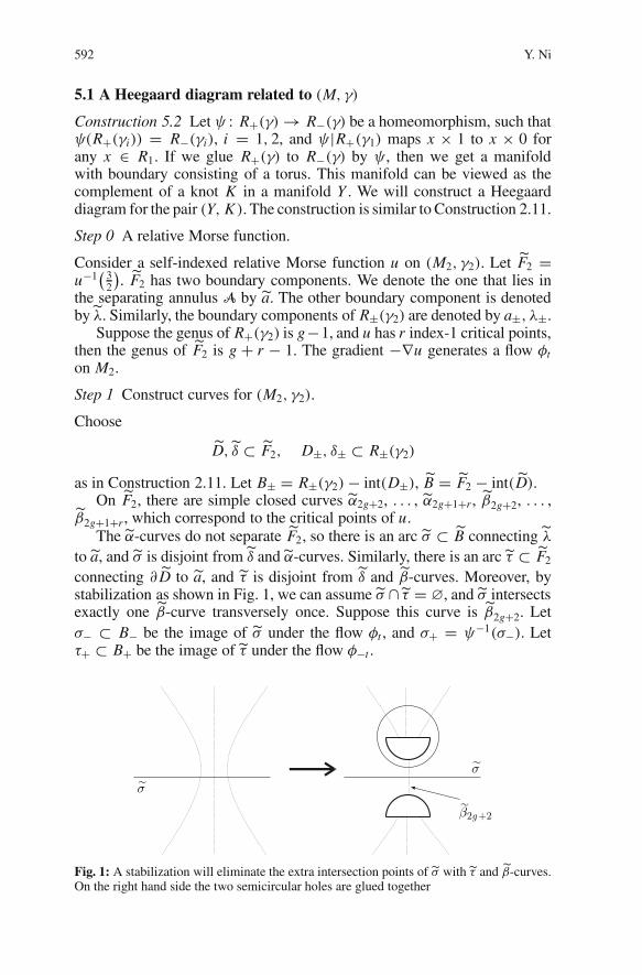
connecting ∂ ˜D to a, and τ is disjoint from ˜δ and ˜β-curves. Moreover, bystabilization as shown in Fig. 1, we can assume σ ∩ τ = ∅, and σ intersectsexactly one ˜β-curve transversely once. Suppose this curve is ˜β2g+2. Letσ− ⊂ B− be the image of σ under the flow φt , and σ+ = ψ−1(σ−). Letτ+ ⊂ B+ be the image of τ under the flow φ−t .
Fig. 1: A stabilization will eliminate the extra intersection points of σ with τ and ˜β-curves.On the right hand side the two semicircular holes are glued together
Knot Floer homology detects fibred knots 593
Choose 2g−2 disjoint arcs ξ−4 , . . . , ξ−
2g+1 ⊂ B−, such that their endpointslie on λ−, and they are linearly independent in H1(B−, ∂B−). We alsosuppose they are disjoint from δ− , σ− and the bad points. Let ξ+
i = ψ−1(ξ−i ).
We also flow back ξ−4 , . . . , ξ−
2g+1 by φ−t to ˜F2, the images are denotedby ˜ξ4, . . . , ˜ξ2g+1.
Choose 2g−2 disjoint arcs η+4 , . . . , η+
2g+1 ⊂ B+, such that their endpointslie on ∂D+, and they are linearly independent in H1(B+, ∂B+). We alsosuppose they are disjoint from δ+, τ+ and the bad points. Flow them by φt
to ˜F, the images are denoted by η4, . . . , η2g+1.We can slide η-curves over ˜β2g+2 to eliminate the possible intersection
points between η-curves and σ .By stabilization, we can assume τ does not intersect ˜ξ-curves, and it
intersects exactly one α-curve transversely once. This curve is denotedby α2g+2.
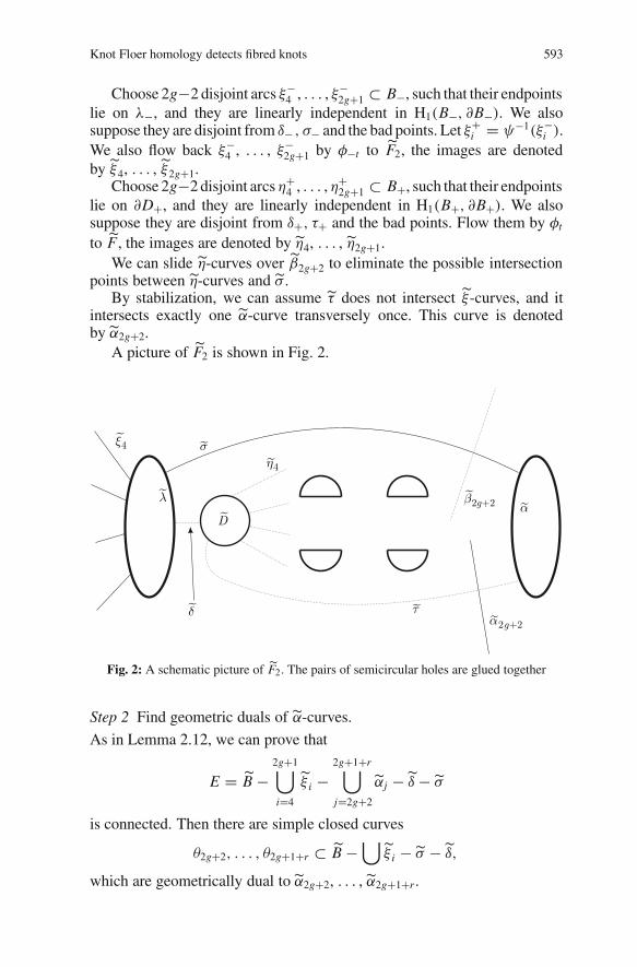
A picture of ˜F2 is shown in Fig. 2.
Fig. 2: A schematic picture of ˜F2. The pairs of semicircular holes are glued together
Step 2 Find geometric duals of α-curves.
As in Lemma 2.12, we can prove that
E = ˜B −2g+1⋃
i=4
˜ξ i −2g+1+r⋃
j=2g+2
αj −˜δ − σ
is connected. Then there are simple closed curves
θ2g+2, . . . , θ2g+1+r ⊂ ˜B −⋃
˜ξ i − σ −˜δ,
which are geometrically dual to α2g+2, . . . , α2g+1+r .
594 Y. Ni
We can slide ˜θ2g+3, . . . , ˜θ2g+1+r over α2g+2 to eliminate the possibleintersection points between˜θ2g+3, . . . ,˜θ2g+1+r and τ .
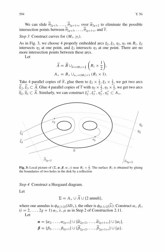
Step 3 Construct curves for (M1, γ1).
As in Fig. 3, we choose 4 properly embedded arcs ξ2, ξ3, η2, η3 on R1. ξ2intersects η2 at one point, and ξ3 intersects η3 at one point. There are nomore intersection points between these arcs.
Let
˜A = ˜B ∪a=(∂R1)× 12
(
R1 × 1
2
)
,
A+ = B+ ∪a+=(∂R1)×1 (R1 × 1).
Take 4 parallel copies of σ , glue them to ξ2 × 12 , ξ3 × 1
2 , we get two arcs˜ξ2,˜ξ3 ⊂ ˜A. Glue 4 parallel copies of τ with η2 × 1
2 , η3 × 12 , we get two arcs
η2, η3 ⊂ ˜A. Similarly, we can construct ξ+2 , ξ+
3 , η+2 , η+
3 ⊂ A+.
Fig. 3: Local picture of (Σ,α,β, w, z) near R1 × 12 . The surface R1 is obtained by gluing
the boundaries of two holes in the disk by a reflection
Step 4 Construct a Heegaard diagram.
Let
Σ = A+ ∪ ˜A ∪ {2 annuli},where one annulus is φ[0,3/2](∂D+), the other is φ[0,3/2](˜λ). Construct αi, βi ,(i = 2, . . . , 2g + 1) α1, λ, µ as in Step 2 of Construction 2.11.
Let
α = {α2, . . . , α2g+1} ∪ {α2g+2, . . . , α2g+1+r} ∪ {α1},β = {β2, . . . , β2g+1} ∪ {˜β2g+2, . . . , ˜β2g+1+r} ∪ {µ}.
Knot Floer homology detects fibred knots 595
Pick two base points w, z near λ ∩ µ, but on different sides of µ. As inConstruction 2.11,
(Σ,α,β, w, z)
is a Heegaard diagram for (Y, K ). ��It is easy to check that the Heegaard diagram constructed above is
a sutured Heegaard diagram. In order to prove our desired result, we stillneed to change the diagram by handleslides.
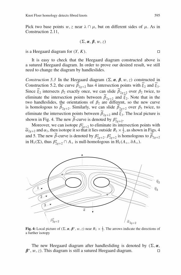
Construction 5.3 In the Heegaard diagram (Σ,α,β, w, z) constructed inConstruction 5.2, the curve ˜β2g+2 has 4 intersection points with ˜ξ2 and ˜ξ3.Since ˜ξ2 intersects β2 exactly once, we can slide ˜β2g+2 over β2 twice, toeliminate the intersection points between ˜β2g+2 and ˜ξ2. Note that in thetwo handleslides, the orientations of β2 are different, so the new curveis homologous to ˜β2g+2. Similarly, we can slide ˜β2g+2 over β3 twice, to
eliminate the intersection points between ˜β2g+2 and ˜ξ3. The local picture isshown in Fig. 4. The new ˜β-curve is denoted by β◦
2g+2.Moreover, we can isotope β◦
2g+2 to eliminate its intersection points withα2g+2 and α1, then isotope it so that it lies outside R1 × 1
2 , as shown in Figs. 4and 5. The new ˜β-curve is denoted by β∗
2g+2. β∗2g+2 is homologous to ˜β2g+2
in H1(Σ), thus β∗2g+2 ∩ A+ is null-homologous in H1(A+, ∂A+).
Fig. 4: Local picture of (Σ,α,β◦, w, z) near R1 × 12 . The arrows indicate the directions of
a further isotopy
The new Heegaard diagram after handlesliding is denoted by (Σ,α,β∗, w, z). This diagram is still a sutured Heegaard diagram. ��
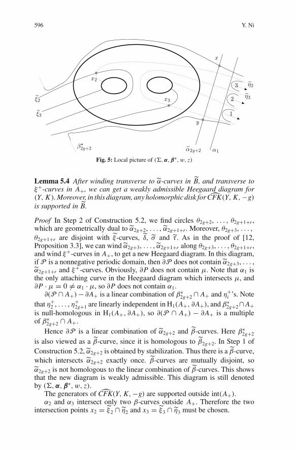
596 Y. Ni
Fig. 5: Local picture of (Σ,α,β∗, w, z)
Lemma 5.4 After winding transverse to α-curves in ˜B, and transverse toξ+-curves in A+, we can get a weakly admissible Heegaard diagram for(Y, K ). Moreover, in this diagram, any holomorphic disk for CFK(Y, K,−g)
is supported in ˜B.
Proof In Step 2 of Construction 5.2, we find circles θ2g+2, . . . , θ2g+1+r ,which are geometrically dual to α2g+2, . . . , α2g+1+r . Moreover, θ2g+3, . . . ,θ2g+1+r are disjoint with ˜ξ-curves, ˜δ, σ and τ . As in the proof of [12,Proposition 3.3], we can wind α2g+3, . . . , α2g+1+r along θ2g+3, . . . , θ2g+1+r ,and wind ξ+-curves in A+, to get a new Heegaard diagram. In this diagram,if P is a nonnegative periodic domain, then ∂P does not contain α2g+3, . . . ,α2g+1+r and ξ+-curves. Obviously, ∂P does not contain µ. Note that α1 isthe only attaching curve in the Heegaard diagram which intersects µ, and∂P · µ = 0 �= α1 · µ, so ∂P does not contain α1.
∂(P ∩ A+)− ∂A+ is a linear combination of β∗2g+2 ∩ A+ and η+
i ’s. Notethat η+
2 , . . . , η+2g+1 are linearly independent in H1(A+, ∂A+), and β∗
2g+2∩ A+is null-homologous in H1(A+, ∂A+), so ∂(P ∩ A+) − ∂A+ is a multipleof β∗
2g+2 ∩ A+.Hence ∂P is a linear combination of α2g+2 and ˜β-curves. Here β∗
2g+2
is also viewed as a ˜β-curve, since it is homologous to ˜β2g+2. In Step 1 ofConstruction 5.2, α2g+2 is obtained by stabilization. Thus there is a ˜β-curve,which intersects α2g+2 exactly once. ˜β-curves are mutually disjoint, soα2g+2 is not homologous to the linear combination of ˜β-curves. This showsthat the new diagram is weakly admissible. This diagram is still denotedby (Σ,α,β∗, w, z).
The generators of CFK(Y, K,−g) are supported outside int(A+).α2 and α3 intersect only two β-curves outside A+. Therefore the two
intersection points x2 = ˜ξ2 ∩ η2 and x3 = ˜ξ3 ∩ η3 must be chosen.
Knot Floer homology detects fibred knots 597
Suppose Φ is a holomorphic disk for CFK(Y, K,−g). Φ ∩ A+ is a rela-tive periodic domain [12, Definition 3.1] in A+. As before, Φ does notcontain any ξ+-curve after winding, so Φ is supported away from λ. Now∂(Φ ∩ A+) − ∂A+ is a linear combination of β∗
2g+2 ∩ A+ and η+i ’s. As in
the second paragraph of this proof, we have that
∂(Φ ∩ A+) − ∂A+ = m(β∗2g+2 ∩ A+).
Φ is supported away from µ, µ intersects α1 at exactly one point, so thecontribution of α1 to ∂Φ is 0. β∗
2g+2 ∩ A+ separates λ from η+2 ∩ α1. The
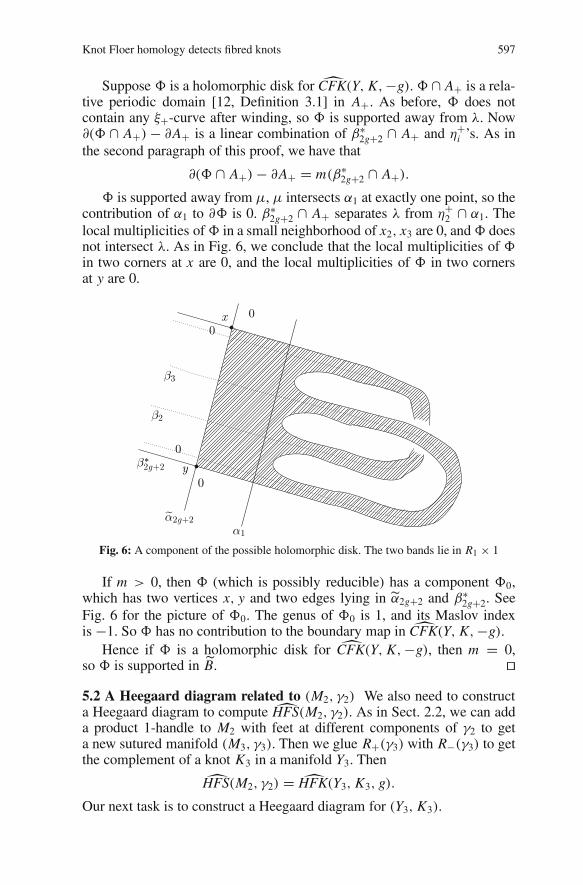
local multiplicities of Φ in a small neighborhood of x2, x3 are 0, and Φ doesnot intersect λ. As in Fig. 6, we conclude that the local multiplicities of Φin two corners at x are 0, and the local multiplicities of Φ in two cornersat y are 0.
Fig. 6: A component of the possible holomorphic disk. The two bands lie in R1 × 1
If m > 0, then Φ (which is possibly reducible) has a component Φ0,which has two vertices x, y and two edges lying in α2g+2 and β∗
2g+2. SeeFig. 6 for the picture of Φ0. The genus of Φ0 is 1, and its Maslov indexis −1. So Φ has no contribution to the boundary map in CFK(Y, K,−g).
Hence if Φ is a holomorphic disk for CFK(Y, K,−g), then m = 0,so Φ is supported in ˜B. ��5.2 A Heegaard diagram related to (M2, γ2) We also need to constructa Heegaard diagram to compute HFS(M2, γ2). As in Sect. 2.2, we can adda product 1-handle to M2 with feet at different components of γ2 to geta new sutured manifold (M3, γ3). Then we glue R+(γ3) with R−(γ3) to getthe complement of a knot K3 in a manifold Y3. Then
HFS(M2, γ2) = HFK(Y3, K3, g).
Our next task is to construct a Heegaard diagram for (Y3, K3).
598 Y. Ni
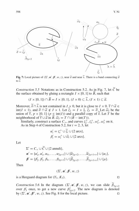
Fig. 7: Local picture of (Σ′,α′,β′, w, z), near a and near ˜λ. There is a band connecting ato˜λ
Construction 5.5 Notations as in Construction 5.2. As in Fig. 7, let ˜C bethe surface obtained by gluing a rectangle I × [0, 1] to ˜B, such that
(I × [0, 1]) ∩ ˜B = I × {0, 1}, (I × 0) ⊂ ˜λ, (I × 1) ⊂ a.
Moreover, ˜δ ∩˜λ is not contained in I × 0, but it is close to I × 0. τ ∩ a ∈int(I × 1), and σ ∩ a /∈ I × 1. Let ˜ζ2 = I × 1
2 , ˜ζ3 = σ . Let ω2 be theunion of τ , p × [0, 1] (p ∈ int(I )) and a parallel copy of ˜δ. Let T be theneighborhood of τ ∪ a in ˜B. ω3 = T ∩ (˜B − int(T )).
Similarly, construct a surface C+, and curves ζ+2 , ζ+
3 , ω+2 , ω+
3 on it.As in Step 4 of Construction 5.2, for i = 2, 3, let
α′i = ζ+
i ∪˜ζi ∪ {2 arcs},β′
i = ω+i ∪ ωi ∪ {2 arcs}.
Let
Σ′ = C+ ∪ ˜C ∪ {2 annuli},α′ = {α′
2, α′3, α4, . . . , α2g+1} ∪ {α2g+2, . . . , α2g+1+r} ∪ {α1},
β′ = {β′2, β
′3, β4, . . . , β2g+1} ∪ {˜β2g+2, . . . , ˜β2g+1+r} ∪ {µ}.
Then
(Σ′,α′,β′, w, z)
is a Heegaard diagram for (Y3, K3). ��Construction 5.6 In the diagram (Σ′,α′,β′, w, z), we can slide ˜β2g+2over β′
3 once, to get a new curve β′′2g+2. The new diagram is denoted
by (Σ′,α′,β′′, w, z). See Fig. 8 for the local picture. ��
Knot Floer homology detects fibred knots 599
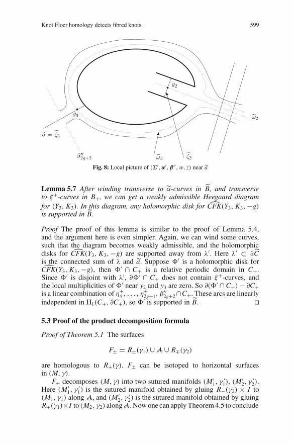
Fig. 8: Local picture of (Σ′,α′,β′′, w, z) near a
Lemma 5.7 After winding transverse to α-curves in ˜B, and transverseto ξ+-curves in B+, we can get a weakly admissible Heegaard diagramfor (Y3, K3). In this diagram, any holomorphic disk for CFK(Y3, K3,−g)is supported in ˜B.
Proof The proof of this lemma is similar to the proof of Lemma 5.4,and the argument here is even simpler. Again, we can wind some curves,such that the diagram becomes weakly admissible, and the holomorphicdisks for CFK(Y3, K3,−g) are supported away from λ′. Here λ′ ⊂ ∂˜Cis the connected sum of λ and a. Suppose Φ′ is a holomorphic disk forCFK(Y3, K3,−g), then Φ′ ∩ C+ is a relative periodic domain in C+.
Since Φ′ is disjoint with λ′, ∂Φ′ ∩ C+ does not contain ξ+-curves, andthe local multiplicities of Φ′ near y2 and y3 are zero. So ∂(Φ′ ∩ C+) − ∂C+is a linear combination of η+
4 , . . . , η+2g+1, β
′′2g+2 ∩C+. These arcs are linearly
independent in H1(C+, ∂C+), so Φ′ is supported in ˜B. ��
5.3 Proof of the product decomposition formula
Proof of Theorem 5.1 The surfaces
F± = R±(γ1) ∪ A ∪ R∓(γ2)
are homologous to R+(γ). F± can be isotoped to horizontal surfacesin (M, γ).
F+ decomposes (M, γ) into two sutured manifolds (M′1, γ
′1), (M′
2, γ′2).
Here (M′1, γ
′1) is the sutured manifold obtained by gluing R−(γ2) × I to
(M1, γ1) along A, and (M′2, γ
′2) is the sutured manifold obtained by gluing
R+(γ1)×I to (M2, γ2) along A. Now one can apply Theorem 4.5 to conclude
600 Y. Ni
that
HFS(M, γ) ∼= HFS(M′1, γ
′1) ⊗ HFS(M′
2, γ′2).
We only need to show that HFS(M′i, γ
′i )
∼= HFS(Mi, γi) for i = 1, 2.Hence we can reduce our theorem to the case that one of the two suturedsubmanifolds M1, M2 is a product.
From now on, we assume M1 is a product.According to Definition 2.2, γ �= ∅. If M1 ∩ γ �= ∅, then one can de-
compose M along product disks to get M2. Now we apply Proposition 2.9(2)to conclude that HFS(M, γ) ∼= HFS(M2, γ2).
Now we consider the case that M1∩γ = ∅. By adding product 1-handleswith feet at γ , we can get a sutured manifold with connected suture.
R+(γ1) contains a subsurface G which is a once-punctured torus. ∂G × Isplits M into two sutured manifolds G × I and (M∗, γ ∗). One can thendecompose M∗ along product disks to get (M2, γ2). Hence we only needto prove the decomposition formula for the case of splitting along ∂G × I .From now on, we focus on this case, namely, the case that the genus ofR+(γ1) is 1.
We apply the constructions in the previous two subsections to getHeegaard diagrams for (Y, K ) and (Y3, K3). See Figs. 5 and 8 for thelocal pictures. For generators of CFK(Y, K,−g), the two intersection pointsx2, x3 in Fig. 5 must be chosen; for generators of CFK(Y3, K3,−g), the twointersection points y2, y3 in Fig. 8 must be chosen. Thus the generators ofCFK(Y, K,−g) and CFK(Y3, K3,−g) are in one-to-one correspondence.
By Lemma 5.4 and Lemma 5.7, the holomorphic disks for these two chaincomplexes are also the same. Hence
HFK(Y, K,−g) = HFK(Y3, K3,−g),
which means that
HFS(M, γ) = HFS(M2, γ2)
by definition. ��
5.4 An application to satellite knots As an application, we can computethe topmost terms in the knot Floer homology of satellite knots with nonzerowinding numbers. We recall the following definition from [12].
Definition 5.8 Suppose K is a null-homologous knot in Y , F is a Seifert sur-face of K (not necessarily of minimal genus). V is a 3-manifold, ∂V = T 2,L ⊂ V is a nontrivial knot. G ⊂ V is a compact connected oriented surfaceso that L is a component of ∂G, and ∂G−L (may be empty) consists of paral-lel essential circles on ∂V . Orientations on these circles are induced fromthe orientation on G, we require that these circles are parallel as orientedones. We glue V to Y − int(Nd(K )), so that any component of ∂G − L isnull-homologous in Y − int(Nd(K )). The new manifold is denoted by Y ∗,
Knot Floer homology detects fibred knots 601
and the image of L in Y ∗ is denoted by K∗. We then say K∗ is a satelliteknot of K , and K a companion knot of K∗. Let p denote the number ofcomponents of ∂G − L , p will be called the winding number of L in V .
Suppose p > 0, F is a minimal genus Seifert surface for K , then a min-imal genus Seifert surface F∗ for K∗ can be obtained as follows: take p paral-lel copies of F, and glue them to a certain surface G in V − int(Nd(L)).We decompose V − int(Nd(L)) along G, the resulting sutured manifold isdenoted by (M(L), γ(L)), where γ(L) consists of p + 1 annuli, p of themlie on ∂V , denoted by A1, . . . , Ap.
Corollary 5.9 With notations as above, suppose the genus of K is g > 0,and the genus of K∗ is g∗, then
HFK(Y ∗, K∗, [F∗], g∗) ∼= HFK(Y, K, [F], g) ⊗ HFS(M(L), γ(L))
as linear spaces over any field F.
Proof Let (M, γ) be the sutured manifold obtained by decomposing Y ∗ −int(Nd(K∗)) along F∗. Note that A1, . . . , Ap are separating product annuliin M. The desired result holds by Theorem 5.1. ��
Matthew Hedden also got some interesting results regarding knot Floerhomology of satellite knots with nonzero winding numbers [8]. Our resultcan be compared with his.
6 Characteristic product regions
Definition 6.1 Suppose (M, γ) is an irreducible sutured manifold, γ hasno toral component, R−(γ), R+(γ) are incompressible and diffeomorphicto each other. A product region for M is a submanifold Φ × I of N, suchthat Φ is a compact, possibly disconnected, surface, and Φ × 0, Φ × 1 areincompressible subsurfaces of R−(γ), R+(γ), respectively.
There exists a product region E × I , such that if Φ × I is any productregion for M, then there is an ambient isotopy of M which takes Φ × Iinto E × I . E × I is called a characteristic product region for M.
The theory of characteristic product regions is actually a part of JSJtheory [9,10], the version that we need in the current paper can be foundin [1].
The following theorem can be abbreviated as: if HFS(M, γ) ∼= Z, thenthe characteristic product region carries all the homology. A version of thistheorem is also proved by Ian Agol via a different approach.
Theorem 6.2 Suppose (M, γ) is an irreducible balanced sutured manifold,γ has only one component, and (M, γ) is vertically prime. Let E × I ⊂ Mbe the characteristic product region for M.
602 Y. Ni
If HFS(M, γ) ∼= Z, then the map
i∗ : H1(E × I ) → H1(M)
is surjective.
By Proposition 3.1, (M, γ) is a homology product.Let G be a genus-1 compact surface with one boundary component. Glue
the two sutured manifolds (M, γ) and G × I together along their verticalboundaries, we get a sutured manifold N with empty suture. N has twoboundary components Σ = Σ− = R−(γ)∪(G×0), Σ+ = R+(γ)∪(G×1).N is also a homology product, thus there is a natural isomorphism
∂∗ : H2(N, ∂N) → H1(Σ).
Remark 6.3 Since (M, γ) is a homology product, we can glue R−(γ)to R+(γ), so that the resulting manifold is the complement of a knot Kin a homology 3-sphere Y �≈ S3. Suppose J is a genus-1 fibred knot ina homology sphere Z �≈ S3, G′ is a fibre. Consider the knot K#J ⊂ Y#Z.Let Y ′
0 be the manifold obtained by 0-surgery on K#J . Let F = R−(γ) ⊂ Y ,H be the boundary connected sum of F and G′, and H be the extensionof H in Y ′
0.If we cut Y ′
0 open along H , then we get the manifold N. [4, The-orem 8.9] shows that Y ′
0 admits a taut foliation, with H as a compact leaf.Thus this foliation induces a foliation of N.
Assume that the map
i∗ : H1(E × I ) → H1(M)
is not surjective. We can find a simple closed curve ω ⊂ R−(γ), such that[ω] is not in i∗(H1(E × I )).
Let ω− = ω ⊂ Σ−, and let ω+ ⊂ Σ+ be a circle homologous to ω.We fix an arc δ connecting Σ− to Σ+. Let Sm(+ω) be the set of properlyembedded surfaces S ⊂ N, such that ∂S = ω− � (−ω+), and the algebraicintersection number of S with δ is m. Here −ω+ denotes the curve ω+,but with opposite orientation. Similarly, let Sm(−ω) be the set of properlyembedded surfaces S ⊂ N, such that ∂S = (−ω−) � ω+, and the algebraicintersection number of S with δ is m. Let x(Sm(±ω)) be the minimal valueof x(S) for all S ∈ Sm(±ω). It is obvious that
x(Sm+1(±ω)) ≤ x(Sm(±ω)) + x(Σ).
The next fact is implicitly contained in [2, Theorem 3.13].
Lemma 6.4 When m is sufficiently large, there exist connected surfacesS1 ∈ Sm(+ω) and S2 ∈ Sm(−ω), such that they give taut decompositionsof N.
Knot Floer homology detects fibred knots 603
Proof Let D(N) be the double of N along ∂N. a = ∂−1∗ ([ω]) ∈ H2(N, ∂N)is the homology class whose intersection with Σ is [ω], D(a) is its doublein H2(D(N)). There exists C ≥ 0, such that if k > C, then x(D(a)+(k+1)[Σ]) = x(D(a)+k[Σ])+x(Σ). As in the proof of [2, Theorem 3.13],if Q is a Thurston norm minimizing surface in the homology class D(a) +k[Σ], and Q ∩ N has no disk or sphere components, then Q ∩ N gives a tautdecomposition of N.
We can do oriented cut-and-paste of Q with copies of Σ, to get a newsurface Q′, such that Q′ ∩ N has positive intersection number with δ. Ofcourse, Q′∩N still gives a taut decomposition of N . The not-so-good thing isthat ∂(Q′∩ N) is not necessarily ω−�(−ω+). What we can do is to apply [3,Lemma 0.6]. Note that in the proof of [3, Lemma 0.6], one gets a newdecomposition surface with prescribed boundary by gluing subsurfaces Wiof Σ± to the original decomposition surface. And by [2, Lemma 3.10],Wi has the same orientation as Σ±. So the algebraic intersection number ofthis new decomposition surface with δ is no less than (Q′ ∩ N) · δ > 0.
Denote the new decomposition surface by S0, ∂S0 = ω− � (−ω+).Suppose S1 is the component of S0 which contains ω−. For homologicalreason, S1 should also contain −ω+. Thus other components of S0 areclosed surfaces which do not separate Σ− from Σ+. Hence the algebraicintersection number of other components with δ is 0. S1 also gives a tautdecomposition of N, by [3, Lemma 0.4]. So S1 is the surface we need.Similarly, we can prove the result for Sm(−ω). ��
We also need the following key lemma.
Lemma 6.5 For any positive integers p, q,
x(Sp(+ω)) + x(Sq(−ω)) > (p + q)x(Σ).
Suppose S1 ∈ Sp(+ω), S2 ∈ Sq(−ω). Isotope S1, S2 so that they are trans-verse. Since N is irreducible and S1, S2 are incompressible, we can assumeS1 ∪ S2 − S1 ∩ S2 has no disk components. Perform oriented cut-and-pasteto S1, S2, we get a closed surface P ⊂ int(N), with x(P) = x(S1) + x(S2).P has no sphere components, otherwise S1 ∪ S2 − S1 ∩ S2 would have diskcomponents.
Now we will deal with the possible toral components of P. To this end,we need the following lemma.
Lemma 6.6 If T ⊂ int(N) is a torus, then the algebraic intersectionnumber of T and δ is 0.
Proof Since N is a homology product, we have
H2(D(N)) ∼= H2(Σ) ⊕ H1(Σ).
T is disjoint from Σ, so [T ] must be a multiple of [Σ] in H2(D(N)). ByRemark 6.3, Σ is Thurston norm minimizing. Since x(Σ) > 0 = x(T ), wemust have [T ] = 0. Hence T · δ = 0. ��
604 Y. Ni
Suppose T is a toral component of P, then T is the union of 2m annuliA1, A2, . . . , A2m , where A2i−1 ⊂ S1, A2i ⊂ S2. Let
S′1 =
(
S1 −m
⋃
i=1
A2i−1
)
∪m
⋃
i=1
(−A2i),
S′2 =
(
S2 −m
⋃
i=1
A2i
)
∪m
⋃
i=1
(−A2i−1).
Here −Aj means Aj with opposite orientation.A small isotopy will arrange that |S′
1 ∩ S′2| < |S1 ∩ S2|. Moreover,
x(S′1) = x(S1), x(S′
2) = x(S2). We want to show that S′1 ∈ Sp(ω), S′
2 ∈Sq(−ω). Obviously, ∂S′
1 = ∂S1 = ω− � (−ω+), ∂S′2 = ∂S2 = (−ω−) � ω+.
Lemma 6.6 shows that S′1 · δ = S1 · δ. Thus S′
1 ∈ Sp(+ω). Similarly,S′
2 ∈ Sq(−ω). Therefore, we can replace S1, S2 with S′1, S′
2, then continueour argument.
Now we can assume P has no toral components, and proceed to theproof of Lemma 6.5. Our approach to this lemma was suggested by DavidGabai. In fact, this argument is similar to the argument in [4, Lemma 8.22].
Proof of Lemma 6.5 If x(Sp(+ω))+x(Sq(−ω)) ≤ (p+q)x(Σ), then we canget a surface P ⊂ int(N) as above, x(P) ≤ (p + q)x(Σ). Define a functionϕ : (N − P) → Z as follows. When z ∈ Σ−, ϕ(z) = 0. In general, givenz ∈ N − P, choose a path from Σ− to z, ϕ is defined to be the algebraicintersection number of this path with P.
N has the homology type of Σ, thus any closed curve in N shouldhave zero algebraic intersection number with any closed surface. Thus ϕ iswell-defined. Moreover, the value of ϕ on Σ+ is p + q.
Let Ji be the closure of {x ∈ (N − P) | ϕ(x) = i}, Pi = Ji−1 ∩ Ji . ThusP = ⊔p+q
i=1 Pi , and⋃i−1
k=0 Jk gives a homology between Σ and Pi . Sincex(P) ≤ (p + q)x(Σ), and Σ is Thurston norm minimizing in D(N), wemust have x(Pi) = x(Σ) for each i.
Pi has only one component. Otherwise, suppose Pi = Q1 � Q2, then
x(Q1), x(Q2) < x(Pi) = x(Σ).
As in the proof of Lemma 6.6, we find that [Q1], [Q2] are multiples of [Σ],which gives a contradiction.
We can isotope P, so that Pi ∩ M is a genus g surface with one boundarycomponent. In fact, after an isotopy, we can arrange that P ∩ γ1 consists ofparallel essential curves in γ1. Since F and G are Thurston norm minimizingin H2(M, γ) and H2(G × I, ∂G × I ), respectively, we must have
x(Pi ∩ M) = x(F), x(Pi ∩ (G × I )) = x(G) = 1.
If an annulus A is a component of Pi ∩ (G × I ), then we can isotope Ainside G × I into ∂G × I , a further isotopy of P will decrease the number
Knot Floer homology detects fibred knots 605
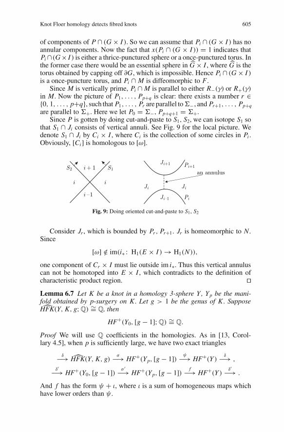
of components of P ∩ (G × I ). So we can assume that Pi ∩ (G × I ) has noannular components. Now the fact that x(Pi ∩ (G × I )) = 1 indicates thatPi ∩(G× I ) is either a thrice-punctured sphere or a once-punctured torus. Inthe former case there would be an essential sphere in G × I , where G is thetorus obtained by capping off ∂G, which is impossible. Hence Pi ∩ (G × I )is a once-puncture torus, and Pi ∩ M is diffeomorphic to F.
Since M is vertically prime, Pi ∩ M is parallel to either R−(γ) or R+(γ)in M. Now the picture of P1, . . . , Pp+q is clear: there exists a number r ∈{0, 1, . . . , p+q}, such that P1, . . . , Pr are parallel to Σ− , and Pr+1, . . . , Pp+qare parallel to Σ+. Here we let P0 = Σ−, Pp+q+1 = Σ+.
Since P is gotten by doing cut-and-paste to S1, S2, we can isotope S1 sothat S1 ∩ Ji consists of vertical annuli. See Fig. 9 for the local picture. Wedenote S1 ∩ Ji by Ci × I , where Ci is the collection of some circles in Pi .Obviously, [Ci] is homologous to [ω].
Fig. 9: Doing oriented cut-and-paste to S1, S2
Consider Jr , which is bounded by Pr , Pr+1. Jr is homeomorphic to N.Since
[ω] /∈ im(i∗ : H1(E × I ) → H1(N)),
one component of Cr × I must lie outside im i∗. Thus this vertical annuluscan not be homotoped into E × I , which contradicts to the definition ofcharacteristic product region. ��Lemma 6.7 Let K be a knot in a homology 3-sphere Y , Yp be the mani-fold obtained by p-surgery on K. Let g > 1 be the genus of K. SupposeHFK(Y, K, g;Q) ∼= Q, then
HF+(Y0, [g − 1];Q) ∼= Q.
Proof We will use Q coefficients in the homologies. As in [13, Corol-lary 4.5], when p is sufficiently large, we have two exact triangles
δ−→ HFK(Y, K, g)σ−→ HF+(Yp, [g − 1]) ψ−→ HF+(Y )
δ−→ ,
δ′−→ HF+(Y0, [g − 1]) σ ′−→ HF+(Yp, [g − 1]) f−→ HF+(Y )δ′−→ .
And f has the form ψ + ι, where ι is a sum of homogeneous maps whichhave lower orders than ψ.
606 Y. Ni
Since HFK(Y, K, g;Q) ∼= Q, either δ is surjective or σ is injective.Therefore, either ψ is injective, or ψ is surjective. For simplicity, denoteHF+(Yp, [g − 1]) by A, and HF+(Y ) by B.
If ψ is injective, B can be written as ψ(A) ⊕ C for some subgroup Cof B. If b ∈ B is in the form of (ψ(a), c), then let ρ(b) = a. Thus ρ isa homomorphism, ρψ = id, and ιρ : B → B is a homomorphism whichstrictly decreases degree. Now
id −ιρ + (ιρ)2 − (ιρ)3 + · · ·is a well-defined homomorphism and
ψ = (id −ιρ + (ιρ)2 − (ιρ)3 + · · · )(ψ + ι).
Hence f = ψ + ι is also injective, and HF+(Y0, [g − 1]) ∼= B/ f(A).It is easy to check that id +ιρ induces a homomorphism from B/ψ(A)
to B/ f(A), whose inverse is induced by
id −ιρ + (ιρ)2 − (ιρ)3 + · · · .
Thus B/ f(A) ∼= B/ψ(A). So rank(HF+(Y0, [g − 1])) = 1.A similar argument shows that if ψ is surjective, then f is also surjective,
and rank(HF+(Y0, [g − 1])) = 1. ��Proof of Theorem 6.2 Use the notations in Remark 6.3, we have
rank( HFK(Y#Z, K#J, g + 1)) = rank( HFK(Y, K, g)) = 1.
Thus rank(HF+(Y ′0, g)) = 1 by Lemma 6.7.
If i∗ is not surjective, then the proof of [5, Theorem 1.4], combined withLemma 6.4 and Lemma 6.5, shows that
rank(HF+(Y ′0, g)) > 1,
which gives a contradiction.More precisely, by Lemma 6.4 and Lemma 6.5, there exist connected
surfaces S1 ∈ Sm(+ω) and S2 ∈ Sm(−ω), such that they give taut decom-positions of N, and x(S1)+ x(S2) > 2mx(Σ). By Gabai’s work [2, Sect. 5],there exist two taut foliations F1, F2 of N, such that
χ(S1) = e(F1, S1) = e(F1, S0) + mχ(Σ),
χ(S2) = e(F2, S2) = e(F2,−S0) + mχ(Σ).
Here e(F , S) is defined in [5, Definition 3.7], S0 is any surface in S0(+ω).Now we can conclude that e(F1, S0) �= e(F2, S0). Hence [5, The-
orem 3.8] can be applied. ��
Knot Floer homology detects fibred knots 607
7 Proof of the main theorem
Proof of Theorem 1.1 Suppose (M, γ) is the sutured manifold obtained bycutting open Y − int(Nd(K )) along F, E × I is the characteristic productregion. We need to show that M is a product. By Proposition 3.1, M isa homology product. Moreover, by Theorem 4.1, we can assume M isvertically prime.
If M is not a product, then M− E× I is nonempty. Thus there exist someproduct annuli in (M, γ), which split off E × I from M. Let (M′, γ ′) be theremaining sutured manifold. By Theorem 6.2, R±(γ ′) are planar surfaces,and M′ ∩ (E × I ) consists of separating product annuli in M. Since weassume that M is vertically prime, M′ must be connected. (See the firstparagraph in the proof of Theorem 5.1.) Moreover, M′ is also verticallyprime, and there are no nontrivial product disks or product annuli in M′. ByTheorem 5.1, HFS(M′, γ ′) ∼= Z.
We add some product 1-handles to M′ to get a new sutured manifold(M′′, γ ′′) with γ ′′ connected. By Proposition 2.9, HFS(M′′, γ ′′) ∼= Z. It iseasy to see that M′′ is also vertically prime. Proposition 3.1 shows that M′′is a homology product.
In the manifold M′′, the characteristic product region E ′′ × I is the unionof the product 1-handles and Nd(γ ′). Obviously i∗ : H1(E ′′) → H1(M′′) isnot surjective, which contradicts to Theorem 6.2. ��Proof of Corollary 1.2 Cut Y − int(Nd(L)) open along F, we get a suturedmanifold (M, γ), HFS(M, γ) ∼= Z. By adding product 1-handles with feetat γ , we can get a new sutured manifold (M′, γ ′), where γ ′ has only onecomponent. We have HFS(M′, γ ′) ∼= Z. By Theorem 1.1, M′ is a product,hence M is also a product. So the desired result holds. ��
References
1. Cooper, D., Long, D.: Virtually Haken Dehn-filling. J. Differ. Geom. 52(1), 173–187(1999)
2. Gabai, D.: Foliations and the topology of 3-manifolds. J. Differ. Geom. 18(3), 445–503(1983)
3. Gabai, D.: Foliations and the topology of 3-manifolds II. J. Differ. Geom. 26(3), 461–478 (1987)
4. Gabai, D.: Foliations and the topology of 3-manifolds III. J. Differ. Geom. 26(3),479–536 (1987)
5. Ghiggini, P.: Knot Floer homology detects genus-one fibred knots. preprint (2006). Toappear in Amer. J. Math., arXiv: math.GT/0603445
6. Goda, H.: Heegaard splitting for sutured manifolds and Murasugi sum. Osaka J. Math.29(1), 21–40 (1992)
7. Grigsby, E.: Knot Floer Homology in cyclic branched covers, Algebr. Geom. Topol. 6,1355–1398 (2006) (electronic)
8. Hedden, M.: private communication9. Jaco, W., Shalen, P.: Seifert Fibered Spaces in 3-Manifolds. Mem. Am. Math. Soc.,
vol. 21, no. 220. Am. Math. Soc., Providence, RI (1979)
608 Y. Ni
10. Johannson, K.: Homotopy Equivalences of 3-Manifolds with Boundaries. Lect. NotesMath., vol. 761. Springer, Berlin (1979)
11. Juhasz, A.: Holomorphic discs and sutured manifolds. Algebr. Geom. Topol. 6, 1429–1457 (2006) (electronic)
12. Ni, Y.: Sutured Heegaard diagrams for knots. Algebr. Geom. Topol. 6, 513–537 (2006)(electronic)
13. Ozsvath, P., Szabo, Z.: Holomorphic disks and knot invariants. Adv. Math. 186(1),58–116 (2004)
14. Ozsvath, P., Szabo, Z.: Holomorphic disks and genus bounds. Geom. Topol. 8, 311–334(2004) (electronic)
15. Ozsvath, P., Szabo, Z.: On knot Floer homology and lens space surgeries. Topology44(6), 1281–1300 (2005)
16. Ozsvath, P., Szabo, Z.: Heegaard Floer homologies and contact structures. Duke Math. J.129(1), 39–61 (2005)
17. Ozsvath, P., Szabo, Z.: Knot Floer homology and rational surgeries. preprint (2005),arXiv: math.GT/0504404
18. Ozsvath, P., Szabo, Z.: Heegaard diagrams and holomorphic disks. In: Different Facesof Geometry. Int. Math. Ser., N.Y., pp. 301–348. Kluwer/Plenum, New York (2004)
19. Rasmussen, J.: Floer homology and knot complements. PhD Thesis, Harvard University(2003), arXiv: math.GT/0306378
20. Stallings, J.: On fibering certain 3-manifolds. In: Topology of 3-Manifolds and Re-lated Topics. Proc. the Univ. of Georgia Institute (1961), pp. 95–100. Prentice-Hall,Englewood Cliffs, New Jersey (1962)
21. Thurston, W.: A norm for the homology of 3-manifolds. Mem. Am. Math. Soc. 59(339),i–vi, 99–130 (1986)