Instantaneous power p(t) flowing into the box

1

Instantaneous power p(t) flowing into the box

)()()( titvtp Circuit in a box, two wires

)(ti

)(tv+

−

)(ti

)()()()()( titvtitvtp bbaa )(tvaCircuit in a box,

three wires

)(tia+

−

)(tib

+

−)(tvb

)()( titi ba Any wire can be the voltage reference

Works for any circuit, as long as all N wires are accounted for. There must be (N – 1) voltage measurements, and (N – 1) current measurements.

SG_140122_Power_Definitions_and_Transformers_Presentation.ppt

2

Average value ofperiodic instantaneous power p(t)

Tot

otavg dttp

TP )(1

SG_140122_Power_Def

3

Two-wire sinusoidal case

)sin()sin()()()( tItVtitvtp oo

)cos(22

)cos(2

)(1 IVVIdttp

TP

Tot

otavg

),sin()( tVtv o )sin()( tIti o

2

)2cos()cos()( tVItp o

)cos( rmsrmsavg IVP Power factor

Average power

zero average

SG_140122_Power_Def

4

Root-mean squared value of a periodic waveform with period T

Tot

otavg dttp

TP )(1

RVP rms

avg

2

Tot

otrms dttv

TV )(1 22

Apply v(t) to a resistor

Tot

otTot

otTot

otavg dttv

RTdt

Rtv

Tdttp

TP )(1)(1)(1 2

2

Compare to the average power expression

rms is based on a power concept, describing the equivalent voltage that will produce a given average power to a resistor

The average value of the squared voltage

compare

SG_140122_Power_Def

5

Root-mean squared value of a periodic waveform with period T

Tot

otorms dttV

TV )(sin1 222

Tot

oto

oTot

otorms

ttTVdtt

TVV

2

)(2sin2

)(2cos12

222

,2

22 VVrms

Tot

otrms dttv

TV )(1 22

For the sinusoidal case

2VVrms

),sin()( tVtv o

SG_140122_Power_Def

6-100

-80

-60

-40

-20

0

20

40

60

80

100

0 30 60 90 120 150 180 210 240 270 300 330 360

VoltageCurrent

Given single-phase v(t) and i(t) waveforms for a load

• Determine their magnitudes and phase angles

• Determine the average power

• Determine the impedance of the load

• Using a series RL or RC equivalent, determine the R and L or C

SG_140122_Power_Def

7-100

-80

-60

-40

-20

0

20

40

60

80

100

0 30 60 90 120 150 180 210 240 270 300 330 360

VoltageCurrent

Determine voltage and current magnitudes and phase angles

Voltage cosine has peak = 100V, phase angle = -90º

Current cosine has peak = 50A, phase angle = -135º

, 902

100~ VV AI 1352

50~

Using a cosine reference,

Phasors

SG_140122_Power_Def

8

The average power is

)cos(22

IV

Pavg

45cos2

502

100)135(90cos2

502

100avgP

WPavg 1767

SG_140122_Power_Def

9

Voltage – Current Relationships

)(tiR )(tvR

Rtv

ti RR

)()(

)(tvL)(tiLdttdi

LtvL)()(

)(tvC)(tiC

dttdv

CtiC)()(

SG_140122_Power_Def

10

Thanks to Charles Steinmetz, Steady-State AC Problems are Greatly Simplified with Phasor Analysis

(no differential equations are needed)

RIV

ZR

RR ~

~

LjIV

ZL

LL ~

~

CjIV

ZC

CC

1~~

Rtv

ti RR

)()(

dttdi

LtvL)()(

dttdv

CtiC)()(

Resistor

Inductor

Capacitor

Time Domain Frequency Domain

voltage leads current

current leads voltage

SG_140122_Power_Def

11

20100420100

~~

211

21

21

21

21

31

41

2

1 jVV

j

j

21

21

211

21

21

31

41

jjD

Dj

j

V

2

112120100

21

420100

~1

Dj

j

V

20100

211

21

420100

21

~2

V1 V2

Problem 10.17

120100

420100

~~

211

21

21

21

21

31

41

2

1 jVV

j

j

21

21

211

21

21

31

41

jjD

Dj

j

V

2

1121

120100

21

420100

~1

Dj

j

V

1

201002

1121

420100

21

~2

SG_140122_Power_Def

12

c EE411, Problem 10.17 implicit none dimension v_phasor(2), i_injection_phasor(2), y(2,2) complex v_phasor, i_injection_phasor, y, determinant, i0_phasor real pi open(unit=6,file='EE411_Prob_10_17.txt') pi = 4.0 * atan(1.0) y(1,1) = 1.0 / cmplx(0.0,4.0) 1 + 1.0 / 3.0 2 + 1.0 / 2.0 y(1,2) = -1.0 / 2.0 y(2,1) = y(1,2) y(2,2) = 1.0 / 2.0 1 + 1.0 2 + 1.0 / cmplx(0.0,-2.0) i_injection_phasor(1) = 100.0 1 * cmplx(cos(20.0 * pi / 180.0),sin(20.0 * pi / 180.0)) 2 / cmplx(0.0,4.0) i_injection_phasor(2) = 100.0 1 * cmplx(cos(20.0 * pi / 180.0),sin(20.0 * pi / 180.0)) determinant = y(1,1) * y(2,2) - y(1,2) * y(2,1) write(6,*) "determinant, rectangular = ",determinant write(6,*) "determinant, polar = ", cabs(determinant), 1 atan2(aimag(determinant),real(determinant)) * 180.0 / pi write(6,*) v_phasor(1) = (i_injection_phasor(1) * y(2,2) 1 - y(1,2) * i_injection_phasor(2)) / determinant v_phasor(2) = (y(1,1) * i_injection_phasor(2) 1 - i_injection_phasor(1) * y(2,1)) / determinant write(6,*) "v_phasor(1), rectangular = ",v_phasor(1) write(6,*) "v_phasor(1), polar = ", cabs(v_phasor(1)), 1 atan2(aimag(v_phasor(1)),real(v_phasor(1))) * 180.0 / pi write(6,*) write(6,*) "v_phasor(2), rectangular = ",v_phasor(2) write(6,*) "v_phasor(2), polar = ", cabs(v_phasor(2)), 1 atan2(aimag(v_phasor(2)),real(v_phasor(2))) * 180.0 / pi write(6,*) i0_phasor = (v_phasor(1) - v_phasor(2)) / 2.0 write(6,*) "i0_phasor, rectangular = ",i0_phasor write(6,*) "i0_phasor, polar = ", cabs(i0_phasor), 1 atan2(aimag(i0_phasor),real(i0_phasor)) * 180.0 / pi write(6,*) end

SG_140122_Power_Def

13

c EE411, Problem 10.17 implicit none dimension v_phasor(2), i_injection_phasor(2), y(2,2) complex v_phasor, i_injection_phasor, y, determinant, i0_phasor real pi open(unit=6,file='EE411_Prob_10_17.txt') pi = 4.0 * atan(1.0) y(1,1) = 1.0 / cmplx(0.0,4.0) 1 + 1.0 / 3.0 2 + 1.0 / 2.0 y(1,2) = -1.0 / 2.0 y(2,1) = y(1,2) y(2,2) = 1.0 / 2.0 1 + 1.0 2 + 1.0 / cmplx(0.0,-2.0) i_injection_phasor(1) = 100.0 1 * cmplx(cos(20.0 * pi / 180.0),sin(20.0 * pi / 180.0)) 2 / cmplx(0.0,4.0) i_injection_phasor(2) = 100.0 1 * cmplx(cos(20.0 * pi / 180.0),sin(20.0 * pi / 180.0)) determinant = y(1,1) * y(2,2) - y(1,2) * y(2,1) write(6,*) "determinant, rectangular = ",determinant write(6,*) "determinant, polar = ", cabs(determinant), 1 atan2(aimag(determinant),real(determinant)) * 180.0 / pi write(6,*) v_phasor(1) = (i_injection_phasor(1) * y(2,2) 1 - y(1,2) * i_injection_phasor(2)) / determinant v_phasor(2) = (y(1,1) * i_injection_phasor(2) 1 - i_injection_phasor(1) * y(2,1)) / determinant write(6,*) "v_phasor(1), rectangular = ",v_phasor(1) write(6,*) "v_phasor(1), polar = ", cabs(v_phasor(1)), 1 atan2(aimag(v_phasor(1)),real(v_phasor(1))) * 180.0 / pi write(6,*) write(6,*) "v_phasor(2), rectangular = ",v_phasor(2) write(6,*) "v_phasor(2), polar = ", cabs(v_phasor(2)), 1 atan2(aimag(v_phasor(2)),real(v_phasor(2))) * 180.0 / pi write(6,*) i0_phasor = (v_phasor(1) - v_phasor(2)) / 2.0 write(6,*) "i0_phasor, rectangular = ",i0_phasor write(6,*) "i0_phasor, polar = ", cabs(i0_phasor), 1 atan2(aimag(i0_phasor),real(i0_phasor)) * 180.0 / pi write(6,*) end

Program Results determinant, rectangular = (1.125000,4.1666687E-02) determinant, polar = 1.125771 2.121097 v_phasor(1), rectangular = (63.06294,-14.65763) v_phasor(1), polar = 64.74397 -13.08485 v_phasor(2), rectangular = (80.67508,-8.976228) v_phasor(2), polar = 81.17290 -6.348842 i0_phasor, rectangular = (-8.806068,-2.840703) i0_phasor, polar = 9.252914 -162.1211

SG_140122_Power_Def

14

Active and Reactive Power Form a Power Triangle

),cos(22

IV

Pavg ),sin(22

IV

Q

jQPIVS ~ ~

)(

VV~

II~ P

Q

Projection of S on the real axis

Projection of S on the

imaginary axis

Complex power

S

)(

)cos( is the power factorSG_140122_Power_Def

15

Question: Why is there conservation of P and Q in a circuit?

Answer: Because of KCL, power cannot simply vanish but must be accounted for

0~~~~ CBA IIIV

Consider a node, with voltage (to any reference), and three currents

IA IB

IC

0~~~ CBA III

0~~~~ * CBA IIIV

0 CCBBAA jQPjQPjQP

0 CBA PPP

0 CBA QQQ

SG_140122_Power_Def

16

Voltage and Current Phasors for R’s, L’s, C’s

RRR

RR IRVR

IV

Z ~~ ,~~

LLL

LL ILjVLj

IV

Z ~~ ,~~

CjI

VCjI

VZ C

CC

CC

~~ ,1~~

Resistor

Inductor

Capacitor

Voltage and Current in phase Q = 0

Voltage leads Current by 90°

Q > 0

Current leads Voltage by 90° Q < 0

SG_140122_Power_Def

17

VIIVIVjQPS **~~

cosVIP

sinVIQ

P

Q

Projection of S on the real axis

Projection of S on the

imaginary axis

Complex power

S

)(

SG_140122_Power_Def

18

RV

ZV

ZVVjQPS

2

*

2*~~

RIRVP 2

2 0Q

RIZIIZIjQPS 22*~~

also

so

Resistor

, Use rms V, I

SG_140122_Power_Def

19

L

jVLj

V

Lj

VZVVjQPS

22

*

2*~~

LILVQ

22

0P

LjILjIIZIjQPS 22*~~

also

so

Inductor

, Use rms V, I

SG_140122_Power_Def

20

22

*

2*

11

~~ CVj

Cj

V

Cj

VZVVjQPS

CICVQ

2

2 0P

CIj

CjIIZIjQPS

22* 1~~

also

so

Capacitor

, Use rms V, I

SG_140122_Power_Def

21

Active and Reactive Power for R’s, L’s, C’s(a positive value is consumed, a negative value is produced)

0

LIL

Vrms

rms

22

,

RIRV

rmsrms 22

,

0

0

Resistor

Inductor

Capacitor

Active Power P Reactive Power Q

, , 2

2CICV rms

rms

source of reactive power

SG_140122_Power_Def

22

Now, demonstrate Excel spreadsheet

EE411_Voltage_Current_Power.xls

to show the relationship between v(t), i(t), p(t), P, and Q

Vmag = 1Vang = 0Imag = 0.90 90Iang = -30 150

Phase A Phase A Phase A P Q Phase B Phase B Phase B Phase C Phase C Phase C A+B+C Qwt v(t) I(t) p(t) 0.389711 0.225 v(t) I(t) p(t) v(t) I(t) p(t) p(t) 0.675

0 1 0.779423 0.779423 0.389711 0.225 -0.5 -0.779423 0.389711 -0.5 5.51E-17 -2.76E-17 1.169134 0.6752 0.999391 0.794653 0.794169 0.389711 0.225 -0.469472 -0.763243 0.358321 -0.529919 -0.03141 0.016645 1.169134 0.6754 0.997564 0.808915 0.806944 0.389711 0.225 -0.438371 -0.746134 0.327084 -0.559193 -0.062781 0.035107 1.169134 0.6756 0.994522 0.822191 0.817687 0.389711 0.225 -0.406737 -0.728115 0.296151 -0.587785 -0.094076 0.055296 1.169134 0.6758 0.990268 0.834465 0.826345 0.389711 0.225 -0.374607 -0.70921 0.265675 -0.615661 -0.125256 0.077115 1.169134 0.675

10 0.984808 0.845723 0.832875 0.389711 0.225 -0.34202 -0.68944 0.235802 -0.642788 -0.156283 0.100457 1.169134 0.67512 0.978148 0.855951 0.837246 0.389711 0.225 -0.309017 -0.66883 0.20668 -0.669131 -0.187121 0.125208 1.169134 0.67514 0.970296 0.865136 0.839437 0.389711 0.225 -0.275637 -0.647406 0.178449 -0.694658 -0.21773 0.151248 1.169134 0.67516 0.961262 0.873266 0.839437 0.389711 0.225 -0.241922 -0.625193 0.151248 -0.71934 -0.248074 0.178449 1.169134 0.67518 0.951057 0.880333 0.837246 0.389711 0.225 -0.207912 -0.602218 0.125208 -0.743145 -0.278115 0.20668 1.169134 0.67520 0.939693 0.886327 0.832875 0.389711 0.225 -0.173648 -0.578509 0.100457 -0.766044 -0.307818 0.235802 1.169134 0.67522 0.927184 0.891241 0.826345 0.389711 0.225 -0.139173 -0.554095 0.077115 -0.788011 -0.337146 0.265675 1.169134 0.67524 0.913545 0.89507 0.817687 0.389711 0.225 -0.104528 -0.529007 0.055296 -0.809017 -0.366063 0.296151 1.169134 0.67526 0.898794 0.897808 0.806944 0.389711 0.225 -0.069756 -0.503274 0.035107 -0.829038 -0.394534 0.327084 1.169134 0.67528 0.882948 0.899452 0.794169 0.389711 0.225 -0.034899 -0.476927 0.016645 -0.848048 -0.422524 0.358321 1.169134 0.67530 0.866025 0.9 0.779423 0.389711 0.225 6.13E-17 -0.45 -2.76E-17 -0.866025 -0.45 0.389711 1.169134 0.67532 0.848048 0.899452 0.762778 0.389711 0.225 0.034899 -0.422524 -0.014746 -0.882948 -0.476927 0.421102 1.169134 0.67534 0.829038 0.897808 0.744316 0.389711 0.225 0.069756 -0.394534 -0.027521 -0.898794 -0.503274 0.452339 1.169134 0.67536 0.809017 0.89507 0.724127 0.389711 0.225 0.104528 -0.366063 -0.038264 -0.913545 -0.529007 0.483272 1.169134 0.67538 0.788011 0.891241 0.702308 0.389711 0.225 0.139173 -0.337146 -0.046922 -0.927184 -0.554095 0.513748 1.169134 0.675

Instantaneous Power in Single-Phase Circuit

-1.5

0

1.5

0 90 180 270 360 450 540 630 720

vaiapaPQ

Instantaneous Power in Three-Phase Circuit

-1.5

0

1.5

0 90 180 270 360 450 540 630 720

vaiavbibvcicpa+pb+pcQ

SG_140122_Power_Def

23

A load consists of a 47Ω resistor and 10mH inductor in series. The load is energized by a 120V, 60Hz voltage source. The phase angle of the voltage source is zero. a. Determine the phasor current b. Determine the load P, pf, Q, and S. c. Find an expression for instantaneous p(t)

A Single-Phase Power Example

SG_140122_Power_Def

24

A Transmission Line Example

Calculate the P and Q flows (in per unit) for the loadflow situation shown below, and also check conservation of P and Q.

0.05 + j0.15 pu ohms

j0.20 pu mhos

PL + jQL

VL = 1.020 /0° VR = 1.010 /-10° PR + jQR

IS

IcapL IcapRj0.20 pu mhos

SG_140122_Power_Def

25

implicit none complex vl_phasor,sl,icapl_phasor,zcl,is_phasor,zline complex vr_phasor,sr,icapr_phasor,zcr real vlmag,vlang,vrmag,vrang,pi,qcapl,qcapr real vl_mag,vl_ang,vr_mag,vr_ang real rline, xline, bcap real pl,ql,pr,qr,is_mag,is_ang,icapl_mag,icapl_ang,icapr_mag,icapr_ang real qline_loss open(unit=6,file="EE411_Trans_Line.dat") pi = 4.0 * atan(1.0) vl_mag = 1.02 vl_ang = 0.0 vr_mag = 1.01 vr_ang = -10.0 rline = 0.05 xline = 0.15 bcap = 0.20 vl_phasor = vl_mag * cmplx(cos(vl_ang * pi / 180.0),sin(vl_ang * pi / 180.0)) vr_phasor = vr_mag * cmplx(cos(vr_ang * pi / 180.0),sin(vr_ang * pi / 180.0)) is_phasor = (vl_phasor - vr_phasor) / cmplx(rline,xline) icapl_phasor = vl_phasor * cmplx(0.0,bcap) icapr_phasor = vr_phasor * cmplx(0.0,bcap) sl = vl_phasor * conjg(is_phasor + icapl_phasor) sr = vr_phasor * conjg(-is_phasor + icapr_phasor) pl = real(sl) ql = aimag(sl) pr = real(sr) qr = aimag(sr) write(6,*) "is_phasor (rectangular) = ",is_phasor is_mag = cabs(is_phasor) is_ang = atan2(aimag(is_phasor),real(is_phasor)) * 180.0 / pi write(6,*) "is_phasor (polar) ",is_mag,is_ang write(6,*) write(6,*) "icapl_phasor (rectangular) = ",icapl_phasor icapl_mag = cabs(icapl_phasor) icapl_ang = atan2(aimag(icapl_phasor),real(icapl_phasor)) * 180.0 / pi write(6,*) "icapl_phasor (polar) ",icapl_mag,icapl_ang write(6,*) write(6,*) "icapr_phasor (rectangular) = ",icapr_phasor icapr_mag = cabs(icapr_phasor) icapr_ang = atan2(aimag(icapr_phasor),real(icapr_phasor)) * 180.0 / pi write(6,*) "icapr_phasor (polar) ",icapr_mag,icapr_ang write(6,*) qcapl = cabs(vl_phasor) * cabs(vl_phasor) * (-bcap) qcapr = cabs(vr_phasor) * cabs(vr_phasor) * (-bcap) write(6,*) "pl = ",pl write(6,*) "ql = ",ql write(6,*) write(6,*) "pr = ",pr

SG_140122_Power_Def

26

implicit none complex vl_phasor,sl,icapl_phasor,zcl,is_phasor,zline complex vr_phasor,sr,icapr_phasor,zcr real vlmag,vlang,vrmag,vrang,pi,qcapl,qcapr real vl_mag,vl_ang,vr_mag,vr_ang real rline, xline, bcap real pl,ql,pr,qr,is_mag,is_ang,icapl_mag,icapl_ang,icapr_mag,icapr_ang real qline_loss open(unit=6,file="EE411_Trans_Line.dat") pi = 4.0 * atan(1.0) vl_mag = 1.02 vl_ang = 0.0 vr_mag = 1.01 vr_ang = -10.0 rline = 0.05 xline = 0.15 bcap = 0.20 vl_phasor = vl_mag * cmplx(cos(vl_ang * pi / 180.0),sin(vl_ang * pi / 180.0)) vr_phasor = vr_mag * cmplx(cos(vr_ang * pi / 180.0),sin(vr_ang * pi / 180.0)) is_phasor = (vl_phasor - vr_phasor) / cmplx(rline,xline) icapl_phasor = vl_phasor * cmplx(0.0,bcap) icapr_phasor = vr_phasor * cmplx(0.0,bcap) sl = vl_phasor * conjg(is_phasor + icapl_phasor) sr = vr_phasor * conjg(-is_phasor + icapr_phasor) pl = real(sl) ql = aimag(sl) pr = real(sr) qr = aimag(sr) write(6,*) "is_phasor (rectangular) = ",is_phasor is_mag = cabs(is_phasor) is_ang = atan2(aimag(is_phasor),real(is_phasor)) * 180.0 / pi write(6,*) "is_phasor (polar) ",is_mag,is_ang write(6,*) write(6,*) "icapl_phasor (rectangular) = ",icapl_phasor icapl_mag = cabs(icapl_phasor) icapl_ang = atan2(aimag(icapl_phasor),real(icapl_phasor)) * 180.0 / pi write(6,*) "icapl_phasor (polar) ",icapl_mag,icapl_ang write(6,*) write(6,*) "icapr_phasor (rectangular) = ",icapr_phasor icapr_mag = cabs(icapr_phasor) icapr_ang = atan2(aimag(icapr_phasor),real(icapr_phasor)) * 180.0 / pi write(6,*) "icapr_phasor (polar) ",icapr_mag,icapr_ang write(6,*) qcapl = cabs(vl_phasor) * cabs(vl_phasor) * (-bcap) qcapr = cabs(vr_phasor) * cabs(vr_phasor) * (-bcap) write(6,*) "pl = ",pl write(6,*) "ql = ",ql write(6,*) write(6,*) "pr = ",pr write(6,*) "qr = ",qr write(6,*) write(6,*) "qcapl = ",qcapl write(6,*) "qcapr = ",qcapr write(6,*) write(6,*) "pl + pr = ",(pl + pr) write(6,*) "ql + qr = ",(ql + qr) write(6,*) write(6,*) "pline_loss = ",cabs(is_phasor) * cabs(is_phasor) * rline qline_loss = cabs(is_phasor) * cabs(is_phasor) * xline write(6,*) "qline_loss = ",qline_loss write(6,*) "qline_loss + qcapl + qcapr = ",(qline_loss + qcapl + qcapr) write(6,*) end

SG_140122_Power_Def

27

----------------------------------- Results is_phasor (rectangular) = (1.102996,0.1987045) is_phasor (polar) 1.120752 10.21229 icapl_phasor (rectangular) = (0.0000000E+00,0.2040000) icapl_phasor (polar) 0.2040000 90.00000 icapr_phasor (rectangular) = (3.5076931E-02,0.1989312) icapr_phasor (polar) 0.2020000 80.00000 pl = 1.125056 ql = -0.4107586 pr = -1.062252 qr = 0.1870712 qcapl = -0.2080800 qcapr = -0.2040200 pl + pr = 6.2804222E-02 ql + qr = -0.2236874 pline_loss = 6.2804200E-02 qline_loss = 0.1884126 qline_loss + qcapl + qcapr = -0.2236874

0.05 + j0.15 pu ohms

j0.20 pu mhos

PL + jQL

VL = 1.020 /0° VR = 1.010 /-10° PR + jQR

IS

IcapL IcapRj0.20 pu mhos

SG_140122_Power_Def

28

RMS of some common periodic waveforms

22

0

2

0

22 1)(1 DVDTTVdtV

Tdttv

TV

DTT

rms

DVVrms

Duty cycle controller

DT

T

V

0

0 < D < 1By inspection, this is the average value of

the squared waveform

SG_140122_Power_Def

29

RMS of common periodic waveforms, cont.

TTT

rms tTVdtt

TVdtt

TV

TV

03

3

2

0

23

2

0

22

31

T

V

0

3VVrms

Sawtooth

SG_140122_Power_Def

30

RMS of common periodic waveforms, cont.

Using the power concept, it is easy to reason that the following waveforms would all produce the same average power to a resistor, and thus their rms values are identical and equal to the previous example

V

0

V

0

V

0

0

-V

V

0

3VVrms

V

0

V

0

SG_140122_Power_Def

31

2. Three-Phase Circuits

SG_140122_Power_Def

32

Three Important Properties of Three-Phase Balanced Systems

• Because they form a balanced set, the a-b-c currents sum to zero. Thus, there is no return current through the neutral or ground, which reduces wiring losses.

• A N-wire system needs (N – 1) meters. A three-phase, four-wire system needs three meters. A three-phase, three-wire system needs only two meters.

• The instantaneous power is constant

Three-phase, four wire system

abcn

Reference

SG_140122_Power_Def

33

Observe Constant Three-Phase P and Q in Excel spreadsheet

1_Single_Phase_Three_Phase_Instantaneous_Power.xls

Vmag = 1Vang = 0Imag = 0.90 90Iang = -30 150

Phase A Phase A Phase A P Q Phase B Phase B Phase B Phase C Phase C Phase C A+B+C Qwt v(t) I(t) p(t) 0.389711 0.225 v(t) I(t) p(t) v(t) I(t) p(t) p(t) 0.675

0 1 0.779423 0.779423 0.389711 0.225 -0.5 -0.779423 0.389711 -0.5 5.51E-17 -2.76E-17 1.169134 0.6752 0.999391 0.794653 0.794169 0.389711 0.225 -0.469472 -0.763243 0.358321 -0.529919 -0.03141 0.016645 1.169134 0.6754 0.997564 0.808915 0.806944 0.389711 0.225 -0.438371 -0.746134 0.327084 -0.559193 -0.062781 0.035107 1.169134 0.6756 0.994522 0.822191 0.817687 0.389711 0.225 -0.406737 -0.728115 0.296151 -0.587785 -0.094076 0.055296 1.169134 0.6758 0.990268 0.834465 0.826345 0.389711 0.225 -0.374607 -0.70921 0.265675 -0.615661 -0.125256 0.077115 1.169134 0.675

10 0.984808 0.845723 0.832875 0.389711 0.225 -0.34202 -0.68944 0.235802 -0.642788 -0.156283 0.100457 1.169134 0.67512 0.978148 0.855951 0.837246 0.389711 0.225 -0.309017 -0.66883 0.20668 -0.669131 -0.187121 0.125208 1.169134 0.67514 0.970296 0.865136 0.839437 0.389711 0.225 -0.275637 -0.647406 0.178449 -0.694658 -0.21773 0.151248 1.169134 0.67516 0.961262 0.873266 0.839437 0.389711 0.225 -0.241922 -0.625193 0.151248 -0.71934 -0.248074 0.178449 1.169134 0.67518 0.951057 0.880333 0.837246 0.389711 0.225 -0.207912 -0.602218 0.125208 -0.743145 -0.278115 0.20668 1.169134 0.67520 0.939693 0.886327 0.832875 0.389711 0.225 -0.173648 -0.578509 0.100457 -0.766044 -0.307818 0.235802 1.169134 0.67522 0.927184 0.891241 0.826345 0.389711 0.225 -0.139173 -0.554095 0.077115 -0.788011 -0.337146 0.265675 1.169134 0.67524 0.913545 0.89507 0.817687 0.389711 0.225 -0.104528 -0.529007 0.055296 -0.809017 -0.366063 0.296151 1.169134 0.67526 0.898794 0.897808 0.806944 0.389711 0.225 -0.069756 -0.503274 0.035107 -0.829038 -0.394534 0.327084 1.169134 0.67528 0.882948 0.899452 0.794169 0.389711 0.225 -0.034899 -0.476927 0.016645 -0.848048 -0.422524 0.358321 1.169134 0.67530 0.866025 0.9 0.779423 0.389711 0.225 6.13E-17 -0.45 -2.76E-17 -0.866025 -0.45 0.389711 1.169134 0.67532 0.848048 0.899452 0.762778 0.389711 0.225 0.034899 -0.422524 -0.014746 -0.882948 -0.476927 0.421102 1.169134 0.67534 0.829038 0.897808 0.744316 0.389711 0.225 0.069756 -0.394534 -0.027521 -0.898794 -0.503274 0.452339 1.169134 0.67536 0.809017 0.89507 0.724127 0.389711 0.225 0.104528 -0.366063 -0.038264 -0.913545 -0.529007 0.483272 1.169134 0.67538 0.788011 0.891241 0.702308 0.389711 0.225 0.139173 -0.337146 -0.046922 -0.927184 -0.554095 0.513748 1.169134 0.675

Instantaneous Power in Single-Phase Circuit

-1.5

0

1.5

0 90 180 270 360 450 540 630 720

vaiapaPQ

Instantaneous Power in Three-Phase Circuit

-1.5

0

1.5

0 90 180 270 360 450 540 630 720

vaiavbibvcicpa+pb+pcQ

SG_140122_Power_Def

34

The phasors are rotating counter-clockwise. The magnitude of line-to-line voltage phasors is 3 times the magnitude of line-to-neutral voltage phasors.

Vbn

Vab = Van – Vbn

Vbc = Vbn – Vcn

Van

Vcn

30°

120°

Imaginary

Real

Vca = Vcn – Van

SG_140122_Power_Def

35

Conservation of power requires that the magnitudes of delta currents Iab, Ica, and Ibc are 3

1

times the magnitude of line currents Ia, Ib, Ic.

Van

Vbn

Vcn

Real

Imaginary

Vab = Van – Vbn

Vbc = Vbn – Vcn

30°

Vca = Vcn – Van

Ia

Ib

Ic

Iab

Ibc

Ica

Ib

Ic

Iab

Ica

Ibc

Ia

a

c

b

– Vab +

Balanced Sets Add to Zero in Both Time and Phasor Domains

Ia + Ib + Ic = 0

Van + Vbn + Vcn = 0

Vab + Vbc + Vca = 0

Line currents Ia, Ib, and Ic Delta currents Iab, Ibc, and Ica

SG_140122_Power_Def

36

The Two Above Loads are Equivalent in Balanced Systems (i.e., same line currents Ia, Ib, Ic and phase-to-phase voltages Vab, Vbc, Vca in both cases)

3Z

3Z 3Z

a

c

b

– Vab +

Ia

Ib

Ic

Z

Z Z

c

b

– Vab +

Ia

Ib

Ic

n

SG_140122_Power_Def

37

The Two Above Sources are Equivalent in Balanced Systems (i.e., same line currents Ia, Ib, Ic and phase-to-phase voltages Vab, Vbc, Vca in both cases)

a

c

b

– Vab +

Ia

Ib

Ic

Van

a

c

b

– Vab +

Ia

Ib

Ic

n +

–

SG_140122_Power_Def

38

Z

Z Z

a b

– Vab +

Ia

Ib

Ic

c

n In

KCL: In = Ia + Ib + Ic But for a balanced set, Ia + Ib + Ic = 0, so In = 0

Ground (i.e., V = 0)

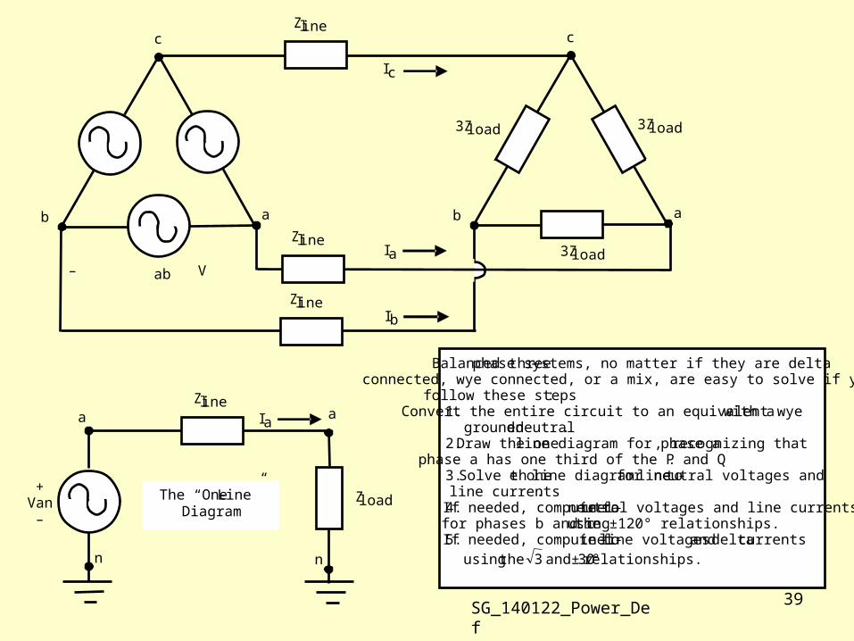
The Experiment: Opening and closing the switch has no effect because In is already zero for a three-phase balanced set. Since no current flows, even if there is a resistance in the grounding path, we must conclude that Vn = 0 at the neutral point (or equivalent neutral point) of any balanced three phase load or source in a balanced system. This allows us to draw a “one- line” diagram (typically for phase a) and solve a single- phase problem.

Solutions for phases b and c follow from the phase shifts that must exist.

SG_140122_Power_Def

39

Balanced three-phase systems, no matter if they are delta connected, wye connected, or a mix, are easy to solve if you follow these steps: 1. Convert the entire circuit to an equivalent wye with a

grounded neutral. 2. Draw the one-line diagram for phase a, recognizing that

phase a has one third of the P and Q. 3. Solve the one-line diagram for line-to-neutral voltages and

line currents. 4. If needed, compute line-to-neutral voltages and line currents

for phases b and c using the ±120° relationships. 5. If needed, compute line-to-line voltages and delta currents

using the 3 and ±30° relationships.

a

n

a

n

Zload +

Van –

Zline Ia

a

c

b

– Vab + 3Zload

a

c

b

Ib

Ia

Ic

Zline

Zline

Zline

3Zload 3Zload

The “One-Line” Diagram

SG_140122_Power_Def

40

Now Work a Three-Phase Motor Power Factor Correction Example

A three-phase, 460V motor draws 5kW with a power factor of 0.80 lagging. Assuming that phasor voltage Van has phase angle zero,

• Find phasor currents Ia and Iab and (note – Iab is inside the motor delta windings)

• Find the three phase motor Q and S

• How much capacitive kVAr (three-phase) should be connected in parallel with the motor to improve the net power factor to 0.95?

• Assuming no change in motor voltage magnitude, what will be the new phasor current Ia after the kVArs are added?

SG_140122_Power_Def

41

Now Work a Delta-Wye Conversion Example

The 60Hz system shown below is balanced. The line-to-line voltage of the source is 460V. Resistors R are each 5Ω. Part a. If each Z is (90 + j45)Ω, determine the three-phase complex power delivered by the source, and the three-phase complex power absorbed by the delta-connected Z loads. Part b. If anV

~ at the source has phase angle zero, find ''~baV at the load.

Z

Z Z

Part c. Draw a phasor diagram that shows line currents Ia, Ib, and Ic, and load currents Iab, Ibc, and Ica.

SG_140122_Power_Def

42

3. Transformers

SG_140122_Power_Def

43

Transformer Core Types

SG_140122_Power_Def

44

High-Voltage Grid Transformers, 100’s of MW

SG_140122_Power_Def

45

Single-Phase Transformer

Rs jXs Ideal

Transformer 7200:240V

Rm jXm

7200V 240V

Turns ratio 7200:240

(30 : 1)

(but approx. same amount of copper in each winding)

Φ

SG_140122_Power_Def

46

Short Circuit Test

Rs jXs Ideal


Rm jXm

7200V 240V



Φ

Short circuit test: Short circuit the 240V-side, and raise the 7200V-side voltage to a few percent of 7200, until rated current flows. There is almost no core flux so the magnetizing terms are negligible.

sc

scss IV

jXR ~~

+Vsc

-

Isc

SG_140122_Power_Def

47

Open Circuit Test

Rs jXs Ideal


Rm jXm

7200V 240V



Φ

+Voc

-

Open circuit test: Open circuit the 7200V-side, and apply 240V to the 240V-side. The winding currents are small, so the series terms are negligible.

oc

ocmm I

VjXR ~

~||

Ioc

SG_140122_Power_Def

48

Single Phase Transformer. Percent values are given on transformer base.

Winding 1kv = 7.2, kVA = 125

Winding 2kv = 0.24, kVA = 125

%imag = 0.5

%loadloss = 0.9

%noloadloss = 0.2

%Xs = 2.2

Rs jXs

Ideal

Transformer

7200:240V Rm jXm

7200V 240V

Magnetizing current

No load loss

XsLoad loss

3. If standard open circuit and short circuit tests are performed on this transformer, what will be the P’s and Q’s (Watts and VArs) measured in those tests?

1. Given the standard percentage values below for a 125kVA transformer, determine the R’s and X’s in the diagram, in Ω.

2. If the R’s and X’s are moved to the 240V side, compute the new Ω values.

SG_140122_Power_Def

49

Rs jXs

Ideal

Transformer

Rm jXm

X / R Ratios for Three-Phase Transformers

• 345kV to 138kV, X/R = 10

• Substation transformers (e.g., 138kV to 25kV or 12.5kV, X/R = 2, X = 12%

• 25kV or 12.5kV to 480V, X/R = 1, X = 5%

• 480V class, X/R = 0.1, X = 1.5% to 4.5%

SG_140122_Power_Def

50

Linear Scale Log10 Scale

Saturation – relative permeability decreases rapidly after 1.7 Tesla

Relative permeability drops from about 2000 to about 1 (becomes air core)

Magnetizing inductance of the core decreases, yielding a highly peaked magnetizing current

SG_140122_Power_Def

51

Transformer Core Saturation

-6

-4

-2

0

2

4

6

Am

pere

s

Magnetizing Current for Single-Phase 25 kVA. 12.5kV/240V Transformer.

THDi = 76.1%, Mostly 3rd Harmonic.

Log10 Scale

Linear Scale

No DC

No DC

With DC

SG_140122_Power_Def

52

Cold Core Test on 1kVA Transformer(120V Winding Excited, 480V Winding Connected to 25 Ohm Resistor, Vdc = 150V on 6500 uF)

MG, March 12, 2009

-20

0

20

40

60

80

100

120

140

160

-0.005 0.000 0.005 0.010 0.015 0.020 0.025

Time - Seconds

Tran

sfor

mer

Cur

rent

in 1

20V

Win

ding

-20

0

20

40

60

80

100

120

140

160

Tran

sfor

mer

Vol

tage

Acr

oss

120V

Win

ding

\

Apply a DC Voltage to a Transformer and Watch It Saturate

Where there is a DC current, there is a DC voltage, and vice-versa

VoltageCurrent

Saturates

SG_140122_Power_Def

53

-0.1

0.0

0.1

0.2

0.3

0.4

0.5

0.6

0.7

0.8

0.9

-150 -100 -50 0 50 100 150 200 250 300

Est. Magnetizing Amps

Volt-

Seco

nds

B-H Curve Constructed from V-I Measurements Shows Linear Region, Saturation, Hysteresis, and Residual Magnetism

Shape of normal hysteresis path

Severe saturation

Severe hysteresis

Residual magnetism

Residual magnetism

SG_140122_Power_Def

Distribution Feeder LossExample• Annual energy loss = 2.40%

• Largest component is transformer no-load loss (45% of the 2.40%)

Transformer No-Load45%

Transformer Load8%

Primary Lines26%

Secondary Lines21%

Annual Loss

Demand values for the peak hour of (load + loss) Total kW % of Consump Total kWh % of ConsumptConsumption/Demand 5665 22222498Total Loss 173 3.06% 534293 2.40%Line Loss (Wires) 123 2.18% 250568 1.13%Transformer Loss (load plus no-load) 50 0.88% 283726 1.28%Load Loss (Wires and transformers) 144 2.54% 291879 1.31%No-Load Loss (Transformer magnetizing) 29 0.52% 242414 1.09%Primary Loss (Includes transformers) 116 2.05% 421316 1.90%Secondary Loss (No transformers) 57 1.01% 112978 0.51%Primary Lines (Wires) 66 1.17% 137590 0.62%Secondary Lines (Wires) 57 1.01% 112978 0.51%No-Load Loss (Transformer magnetizing) 29 0.52% 242414 1.09%Transformer Load Loss 21 0.36% 41312 0.19%

Annual EnergyAt Peak Hour

Modern Distribution Transformer:• Load loss at rated load (I2R in conductors) = 0.75% of rated transformer kW.

• No load loss at rated voltage (magnetizing, core steel) = 0.2% of rated transformer kW.

• Magnetizing current = 0.5% of rated transformer amperes

55

Single-Phase TransformerImpedance Reflection from High-Side (H) to Low-Side (L) by the

Square of the Turns Ratio

Rs jXs Ideal


Rm jXm

7200V 240V

Ideal Transformer 7200:240V

7200V 240V

2

7200240

sjX

2

7200240

sR

2

7200240

mjX2

7200240

mR

2

~/

~

~/

~~

/~

~/

~ ,~

~~~

so ,~~~~

,~~

L

H

L

HH

H

LH

HH

LL

HH

L

H

H

L

H

L

L

HLLHH

L

H

L

HNN

NNI

NNV

IVIVIV

ZZ

NN

VV

IIIVIV

NN

VV

Faraday’s law Conservation of power

SG_140122_Power_Def

56

Now Work a Single-Phase Transformer Example

Open circuit and short circuit tests are performed on a single-phase, 7200:240V, 25kVA, 60Hz distribution transformer. The results are: Short circuit test (short circuit the low-voltage side, energize the high-voltage side so that

rated current flows, and measure Psc and Qsc). Measured Psc = 400W, Qsc = 200VAr. Open circuit test (open circuit the high-voltage side, apply rated voltage to the low-voltage

side, and measure Poc and Qoc). Measured Poc = 100W, Qoc = 250VAr. Determine the four impedance values (in ohms) for the transformer model shown.

Rs jXs Ideal


Rm jXm

7200V 240V


(30 : 1)


Φ

SG_140122_Power_Def

57

Y - Y

A three-phase transformer can be three separate single-phase transformers, or one large transformer with three sets of windings

N1:N2

N1:N2

N1:N2

Rs jXs Ideal

Transformer N1 : N2

Rm jXm

Wye-Equivalent One-Line Model

A

N

• Reflect side 1 wye ohms to side 2 wye ohms by multiplying by [N2 / N1]^2

Standard 345/138kV autotransformers, GY - GY, with a tertiary 12.5kV Δ winding to provide circulating 3rd harmonic current

SG_140122_Power_Def

58

Δ - Δ

For Delta-Delta Connection Model, Convert the Transformer to Equivalent Wye-Wye

N1:N2

N1:N2

N1:N2

Ideal Transformer

3Rs

32 :

31 NN

3jXs

3Rm

3jXm

A

N


• Reflect side 1 delta ohms to side 2 delta ohms by multiplying by [N2 / N1]^2

• Convert side 2 delta ohms to wye ohms by dividing by 3


• Above circuit results in the proper reflection. Note that N2/Sqrt3 divided by N1/Sqrt3 is the same as N2 divided by N1

SG_140122_Power_Def

59Δ - Y

For Delta-Wye Connection Model, Convert the Transformer to Equivalent Wye-Wye

N1:N2

N1:N2

N1:N2

Ideal Transformer

3Rs

2 : 31

NN

3jXs

3Rm

3jXm

A

N


• Reflect side 1 delta ohms to side 2 wye ohms by multiplying by [N2 / N1]^2


• Above circuit results in the proper reflection

Standard building entrance and substation transformers. Δ high side/ GY low side

SG_140122_Power_Def

60

Y - Δ

For Wye-Delta Connection Model, Convert the Transformer to Equivalent Wye-Wye

N1:N2

N1:N2

N1:N2

Ideal Transformer

32 : 1 NN

jXs

Rm jXm

A

N

Rs


So, for all configurations, the equivalent wye-wye transformer ohms can be reflected from one side to the other using the three-phase bank line-to-line turns ratio

• Reflect side 1 wye ohms to side 2 delta ohms by multiplying by [N2 / N1]^2

• Convert side 2 impedances from delta ohms to wye ohms by dividing by 3

• Above circuit results in the proper reflection

SG_140122_Power_Def

61

For wye-delta and delta-wye configurations, there is a phase shift in line-to-line voltages because

• the individual transformer windings on one side are connected line-to-neutral, and on the other side are connected line-to-line

• But there is no phase shift in any of the individual transformers

• This means that line-to-line voltages on the delta side are in phase with line-to-neutral voltages on the wye side

• Thus, phase shift in line-to-line voltages from one side to the other is unavoidable, but it can be managed by standard labeling to avoid problems caused by paralleling transformers

SG_140122_Power_Def

Documents

Instantaneous power p(t) flowing into the box