Derivatives, Instantaneous velocity.

Average and instantaneous rate of change of a function In the last section, we calculated theaverage velocity for a position function s(t), which describes the position of an object ( traveling ina straight line) at time t. We saw that the average velocity over the time interval [t1, t2] is given by

v̄ = s(t2)−s(t1)t2−t1

= ∆s∆t

. This may be interpreted as the average rate of change of the position function s(t)over the interval [t1, t2].

We can apply this general principle to any function given by an equation y = f(x). Note the namesof the independent and dependent variables have changed to x and y in place of t and s above. We candefine the average rate of change of the function f(x) over the interval [x1, x2] as

∆y

∆x=

f(x2)− f(x1)

x2 − x1

.

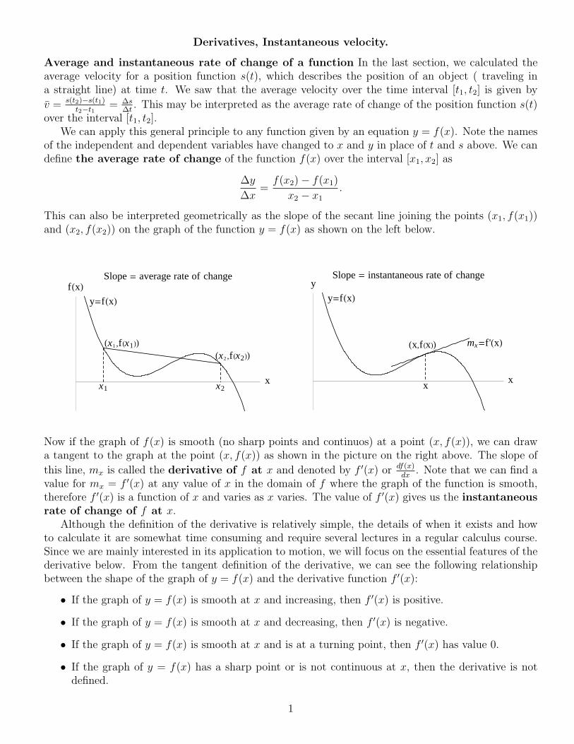
This can also be interpreted geometrically as the slope of the secant line joining the points (x1, f(x1))and (x2, f(x2)) on the graph of the function y = f(x) as shown on the left below.

y=fHxL

Hx1 ,fHx1LLHx2 ,fHx2LL

x2x1x

fHxLSlope = average rate of change

y=fHxL

Hx,fHxLL

x

mx=f'HxL

x

ySlope = instantaneous rate of change

Now if the graph of f(x) is smooth (no sharp points and continuos) at a point (x, f(x)), we can drawa tangent to the graph at the point (x, f(x)) as shown in the picture on the right above. The slope of

this line, mx is called the derivative of f at x and denoted by f ′(x) or df(x)dx

. Note that we can find avalue for mx = f ′(x) at any value of x in the domain of f where the graph of the function is smooth,therefore f ′(x) is a function of x and varies as x varies. The value of f ′(x) gives us the instantaneousrate of change of f at x.

Although the definition of the derivative is relatively simple, the details of when it exists and howto calculate it are somewhat time consuming and require several lectures in a regular calculus course.Since we are mainly interested in its application to motion, we will focus on the essential features of thederivative below. From the tangent definition of the derivative, we can see the following relationshipbetween the shape of the graph of y = f(x) and the derivative function f ′(x):

• If the graph of y = f(x) is smooth at x and increasing, then f ′(x) is positive.

• If the graph of y = f(x) is smooth at x and decreasing, then f ′(x) is negative.

• If the graph of y = f(x) is smooth at x and is at a turning point, then f ′(x) has value 0.

• If the graph of y = f(x) has a sharp point or is not continuous at x, then the derivative is notdefined.

1

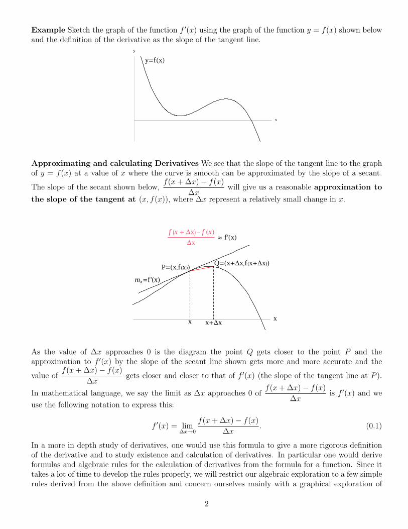
Example Sketch the graph of the function f ′(x) using the graph of the function y = f(x) shown belowand the definition of the derivative as the slope of the tangent line.

y=fHxL

x

y

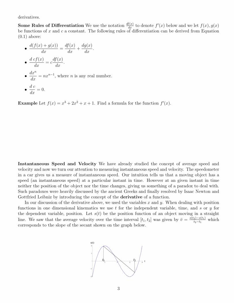
Approximating and calculating Derivatives We see that the slope of the tangent line to the graphof y = f(x) at a value of x where the curve is smooth can be approximated by the slope of a secant.

The slope of the secant shown below,f(x + ∆x)− f(x)

∆xwill give us a reasonable approximation to

the slope of the tangent at (x, f(x)), where ∆x represent a relatively small change in x.

P=Hx,fHxLL Q=Hx+Dx,fHx+DxLL

x

mx=f'HxL

x+Dxx

f Ix + DxM - f HxLDx

» f'HxL

As the value of ∆x approaches 0 is the diagram the point Q gets closer to the point P and theapproximation to f ′(x) by the slope of the secant line shown gets more and more accurate and the

value off(x + ∆x)− f(x)

∆xgets closer and closer to that of f ′(x) (the slope of the tangent line at P ).

In mathematical language, we say the limit as ∆x approaches 0 off(x + ∆x)− f(x)

∆xis f ′(x) and we

use the following notation to express this:

f ′(x) = lim∆x→0

f(x + ∆x)− f(x)

∆x. (0.1)

In a more in depth study of derivatives, one would use this formula to give a more rigorous definitionof the derivative and to study existence and calculation of derivatives. In particular one would deriveformulas and algebraic rules for the calculation of derivatives from the formula for a function. Since ittakes a lot of time to develop the rules properly, we will restrict our algebraic exploration to a few simplerules derived from the above definition and concern ourselves mainly with a graphical exploration of

2

derivatives.

Some Rules of Differentiation We use the notation df(x)dx

to denote f ′(x) below and we let f(x), g(x)be functions of x and c a constant. The following rules of differentiation can be derived from Equation(0.1) above:

• d(f(x) + g(x))

dx=

df(x)

dx+

dg(x)

dx.

• d cf(x)

dx= c

df(x)

dx.

• dxn

dx= nxn−1, where n is any real number.

• d c

dx= 0.

Example Let f(x) = x3 + 2x2 + x + 1. Find a formula for the function f ′(x).

Instantaneous Speed and Velocity We have already studied the concept of average speed andvelocity and now we turn our attention to measuring instantaneous speed and velocity. The speedometerin a car gives us a measure of instantaneous speed. Our intuition tells us that a moving object has aspeed (an instantaneous speed) at a particular instant in time. However at an given instant in timeneither the position of the object nor the time changes, giving us something of a paradox to deal with.Such paradoxes were heavily discussed by the ancient Greeks and finally resolved by Isaac Newton andGottfried Leibniz by introducing the concept of the derivative of a function.

In our discussion of the derivative above, we used the variables x and y. When dealing with positionfunctions in one dimensional kinematics we use t for the independent variable, time, and s or y forthe dependent variable, position. Let s(t) be the position function of an object moving in a straight

line. We saw that the average velocity over the time interval [t1, t2] was given by v̄ = s(t2)−s(t1)t2−t1

whichcorresponds to the slope of the secant shown on the graph below.

t1 t21 2 3 4

t

-2

-1

1

2

sHtL

3

We can estimate the instantaneous speed at time t by taking the average speed in a small time intervalcontaining t. Three different possibilities giving 3 different estimates are shown in the diagrams below,where ∆t represents a small change in t which is positive in this case and the symbol ≈ means “is ap-proximately equal to”. The picture at the right corresponds to ”the central distance method” discussedin your book.

tt-Dtt

sHtL

s Ht - DtL - s HtLDt

» instantaneous rate of change

t t+Dtt

sHtL

s Ht + DtL - s HtLDt

» instantaneous rate of change

t t+Dtt-Dtt

sHtL

s Ht + DtL - s Ht - DtLDt

» instantaneous rate of change

The smaller the value of ∆t in these estimates, the more accurate the estimate will be. It is natural todefine the instantaneous velocity of the object at time t as the limiting value of these estimates as∆t tends to zero (which corresponds to the derivative, s′(t), of the position function at time t and theslope of the tangent to the graph of y = s(t) at t), that is

v(t) = lim∆t→0

s(t + ∆t)− s(t)

∆t= s′(t),

where v(t) denotes the instantaneous velocity of the object at time t.We see, as was the case for general derivatives, that instantaneous velocity changes as time changes

and thus is a function of time. In biomechanics one needs to interpret graphical output and observationaldata in addition to motion which follows a formula as a result of the laws of physics. Therefore, we willdiscuss how to derive an estimate of velocity from graphical output and observational data as well asderiving the velocity function from a position function with a formula.

Instantaneous speed It is not hard to see that for movement of visible objects (where the positionfunction is continuous and smooth), at any given point in time , t, we can choose a ∆t so small thatthe distance travelled by the object on the time interval [t, t + ∆t] is equal to the absolute value ofthe displacement. Therefore when calculating instantaneous speed using the limiting process describedabove for velocity, we get that instantaneous speed at time t is equal to the absolute value of theinstantaneous velocity:

speed at time t = lim∆t→0

|s(t + ∆t)− s(t)|∆t

= |s′(t)| = |v(t)|,

where s(t) denotes the position function of an object moving in a straight line.

Note: Some books on biomechanics use the term velocity to denote speed. One can tell which theymean by how they define the function. Obviously a thorough understanding of the concepts helps yousort out exactly which function they are using independently of how it is labelled.

4

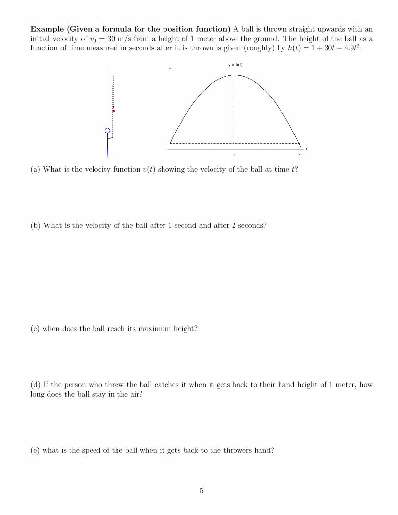
Example (Given a formula for the position function) A ball is thrown straight upwards with aninitial velocity of v0 = 30 m/s from a height of 1 meter above the ground. The height of the ball as afunction of time measured in seconds after it is thrown is given (roughly) by h(t) = 1 + 30t− 4.9t2.

? ?

t

1

y

y = hHtL

(a) What is the velocity function v(t) showing the velocity of the ball at time t?

(b) What is the velocity of the ball after 1 second and after 2 seconds?

(c) when does the ball reach its maximum height?

(d) If the person who threw the ball catches it when it gets back to their hand height of 1 meter, howlong does the ball stay in the air?

(e) what is the speed of the ball when it gets back to the throwers hand?

5

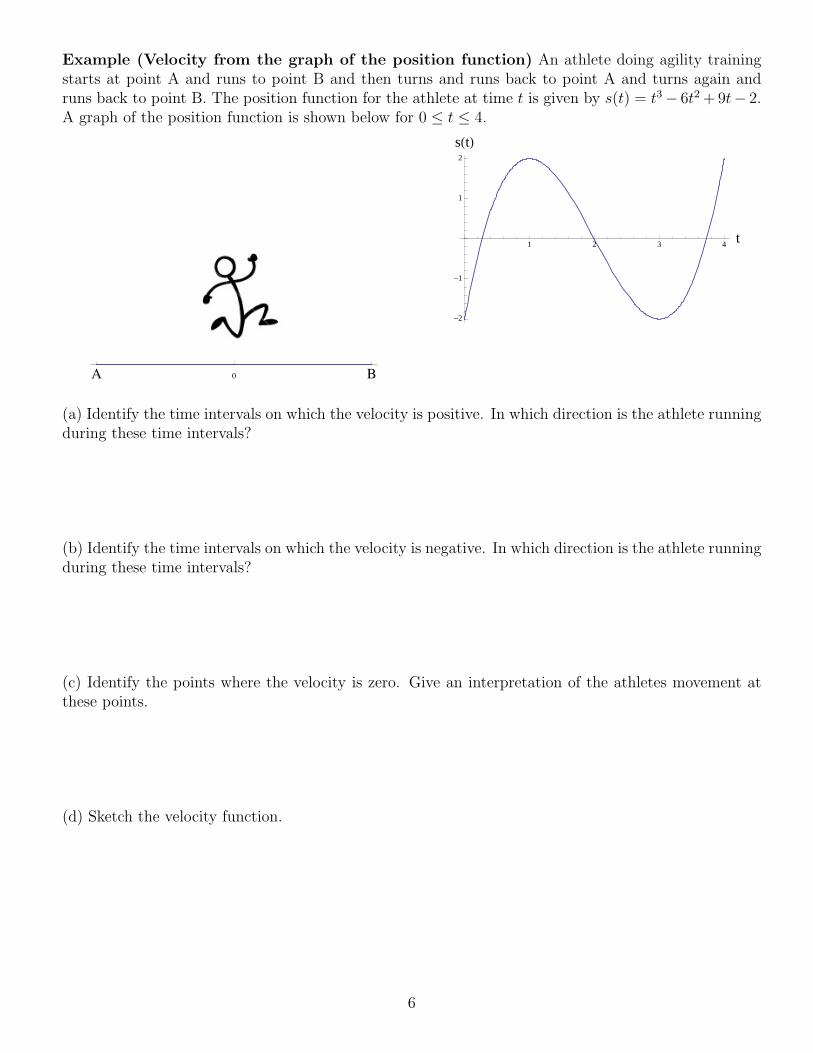
Example (Velocity from the graph of the position function) An athlete doing agility trainingstarts at point A and runs to point B and then turns and runs back to point A and turns again andruns back to point B. The position function for the athlete at time t is given by s(t) = t3− 6t2 + 9t− 2.A graph of the position function is shown below for 0 ≤ t ≤ 4.

0 BA

1 2 3 4t

-2

-1

1

2

sHtL

(a) Identify the time intervals on which the velocity is positive. In which direction is the athlete runningduring these time intervals?

(b) Identify the time intervals on which the velocity is negative. In which direction is the athlete runningduring these time intervals?

(c) Identify the points where the velocity is zero. Give an interpretation of the athletes movement atthese points.

(d) Sketch the velocity function.

6

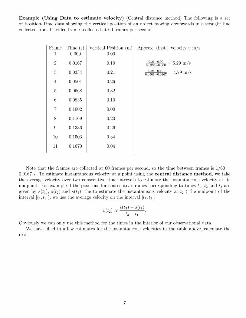
Example (Using Data to estimate velocity) (Central distance method) The following is a setof Position-Time data showing the vertical position of an object moving downwards in a straight linecollected from 11 video frames collected at 60 frames per second.

Frame Time (s) Vertical Position (m) Approx. (inst.) velocity v m/s1 0.000 0.00

2 0.0167 0.10 0.21−0.000.0334−0.000

= 6.29 m/s

3 0.0334 0.21 0.26−0.100.0501−0.0167

= 4.79 m/s

4 0.0501 0.26

5 0.0668 0.32

6 0.0835 0.10

7 0.1002 0.00

8 0.1169 0.20

9 0.1336 0.26

10 0.1503 0.34

11 0.1670 0.04

Note that the frames are collected at 60 frames per second, so the time between frames is 1/60 =0.0167 s. To estimate instantaneous velocity at a point using the central distance method, we takethe average velocity over two consecutive time intervals to estimate the instantaneous velocity at itsmidpoint. For example if the positions for consecutive frames corresponding to times t1, t2 and t3 aregiven by s(t1), s(t2) and s(t3), the to estimate the instantaneous velocity at t2 ( the midpoint of theinterval [t1, t3]), we use the average velocity on the interval [t1, t3]:

v(t2) ≈ s(t3)− s(t1)

t3 − t1

.

Obviously we can only use this method for the times in the interior of our observational data.We have filled in a few estimates for the instantaneous velocities in the table above, calculate the

rest.

7

8

9

10