Embed Size (px)
Citation preview
Installation Effects on Ultrasonic Flow
Meters for Liquids
Jan Drenthen - Krohne
Jan G. Drenthen &
Pico Brand
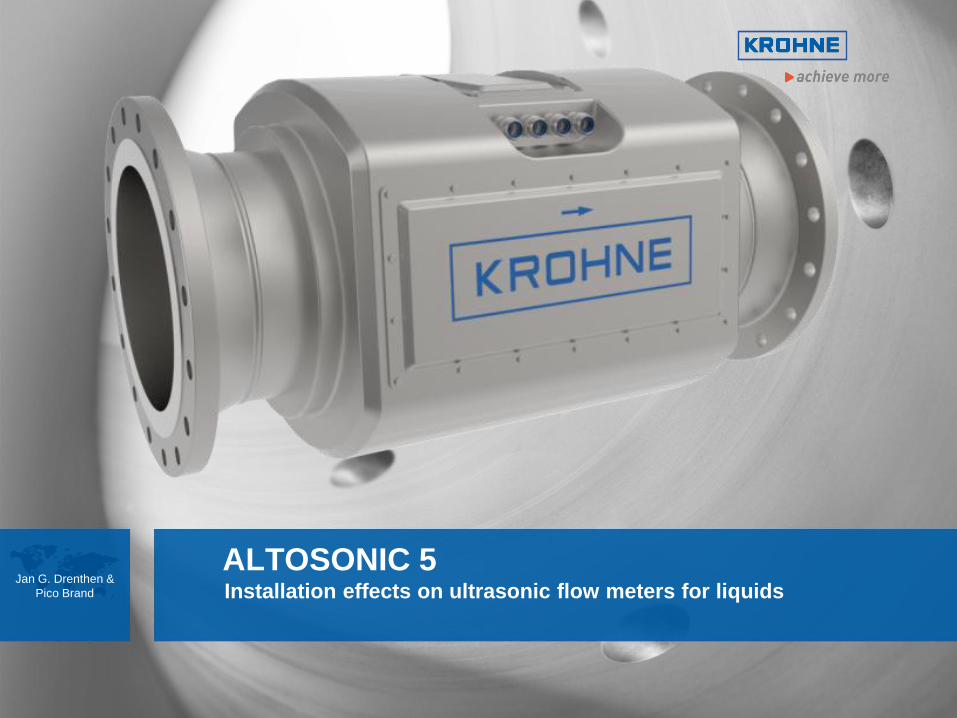
ALTOSONIC 5 Installation effects on ultrasonic flow meters for liquids
Jan G. Drenthen &
Pico Brand
1. Introduction
2. Meter design
3. Test results
• Installation effects
• Meter proving
4. Conclusions
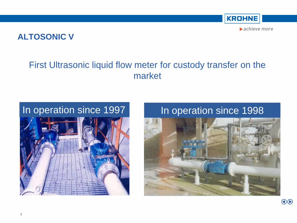
ALTOSONIC V
First Ultrasonic liquid flow meter for custody transfer on the
market
In operation since 1997 In operation since 1998
3
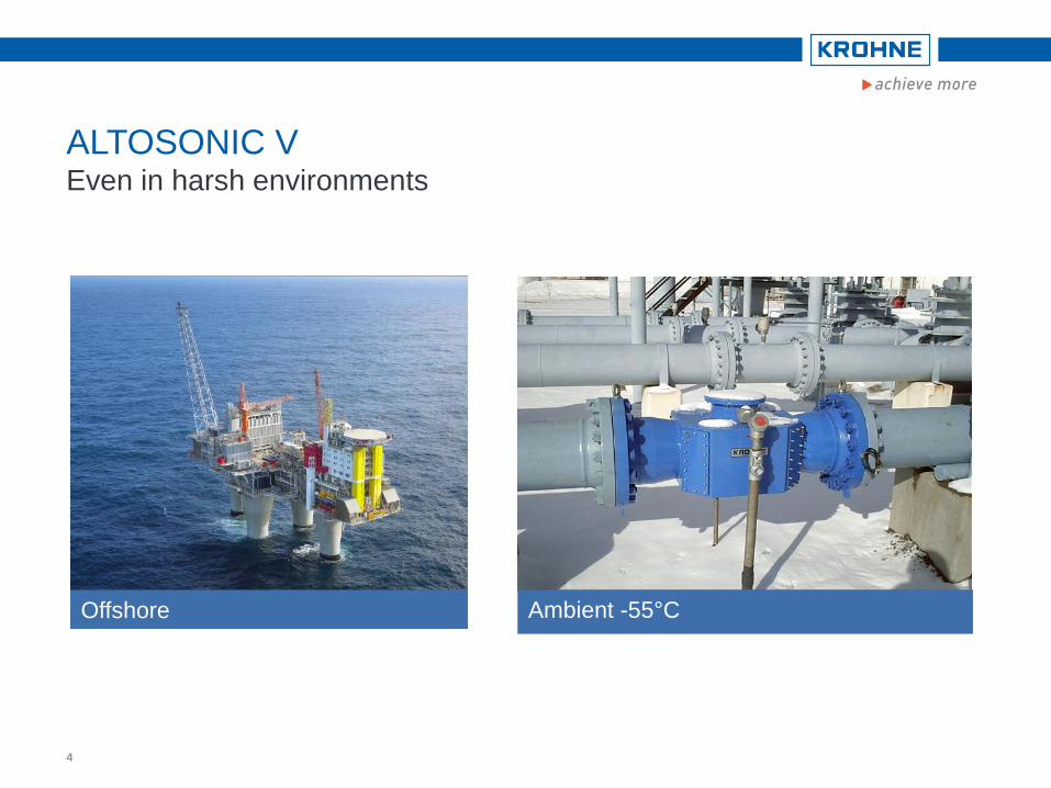
ALTOSONIC V Even in harsh environments
4
Offshore Ambient -55°C
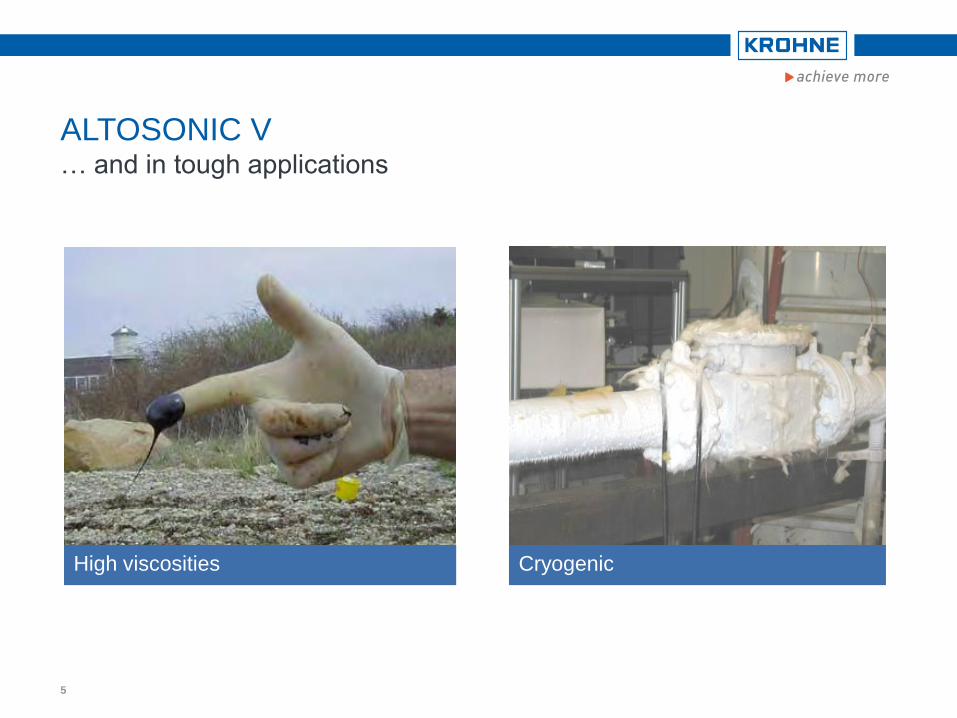
ALTOSONIC V … and in tough applications
5
Cryogenic High viscosities
Pico Brand
2014-04-01
1. Introduction
2. Development of the ALTOSONIC 5
3. Test results
• Installation effects
• Meter proving
4. Conclusions
7
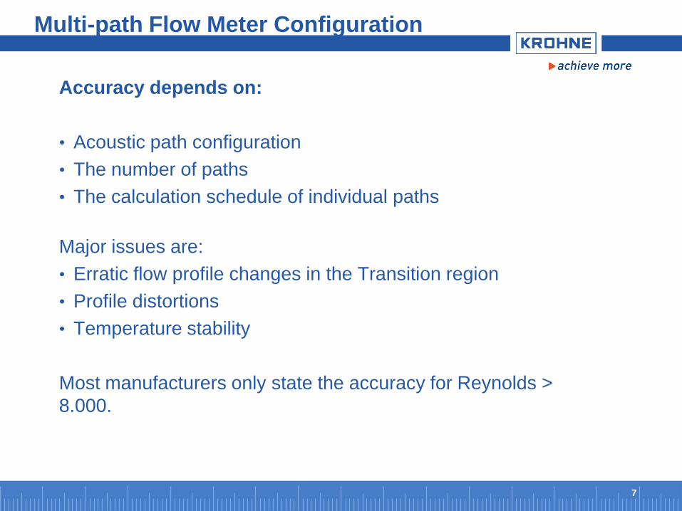
Accuracy depends on:
• Acoustic path configuration
• The number of paths
• The calculation schedule of individual paths
Major issues are:
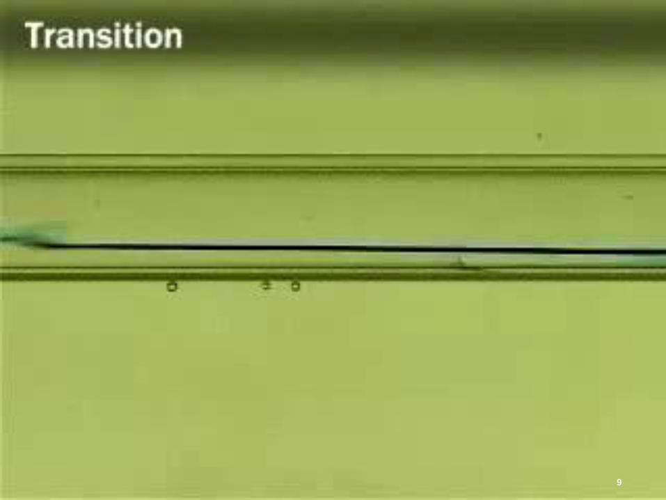
• Erratic flow profile changes in the Transition region
• Profile distortions
• Temperature stability
Most manufacturers only state the accuracy for Reynolds >
8.000.
Multi-path Flow Meter Configuration
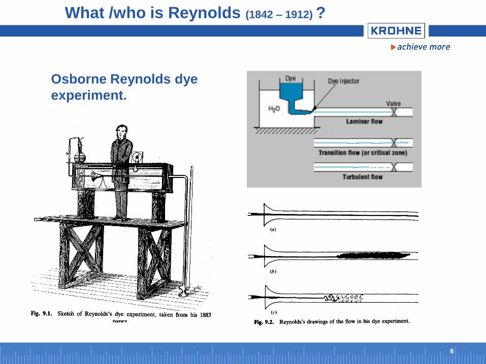
Osborne Reynolds dye
experiment.
8
What /who is Reynolds (1842 – 1912) ?
9
10
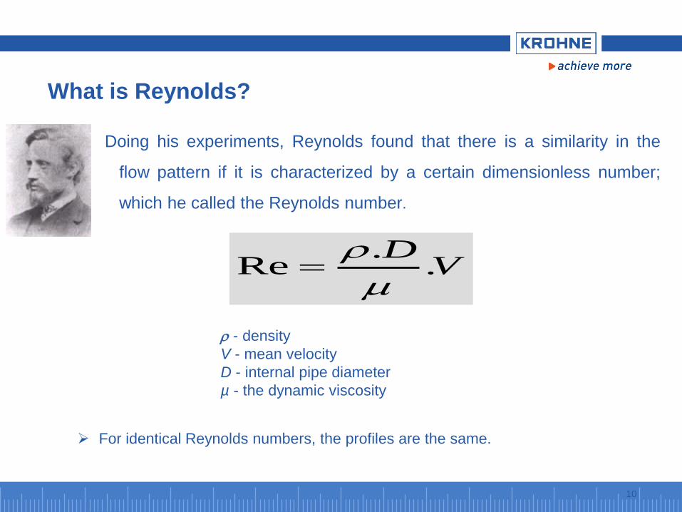
What is Reynolds?
Doing his experiments, Reynolds found that there is a similarity in the
flow pattern if it is characterized by a certain dimensionless number;
which he called the Reynolds number.
VD
..
Re
- density
V - mean velocity
D - internal pipe diameter
µ - the dynamic viscosity
For identical Reynolds numbers, the profiles are the same.
11
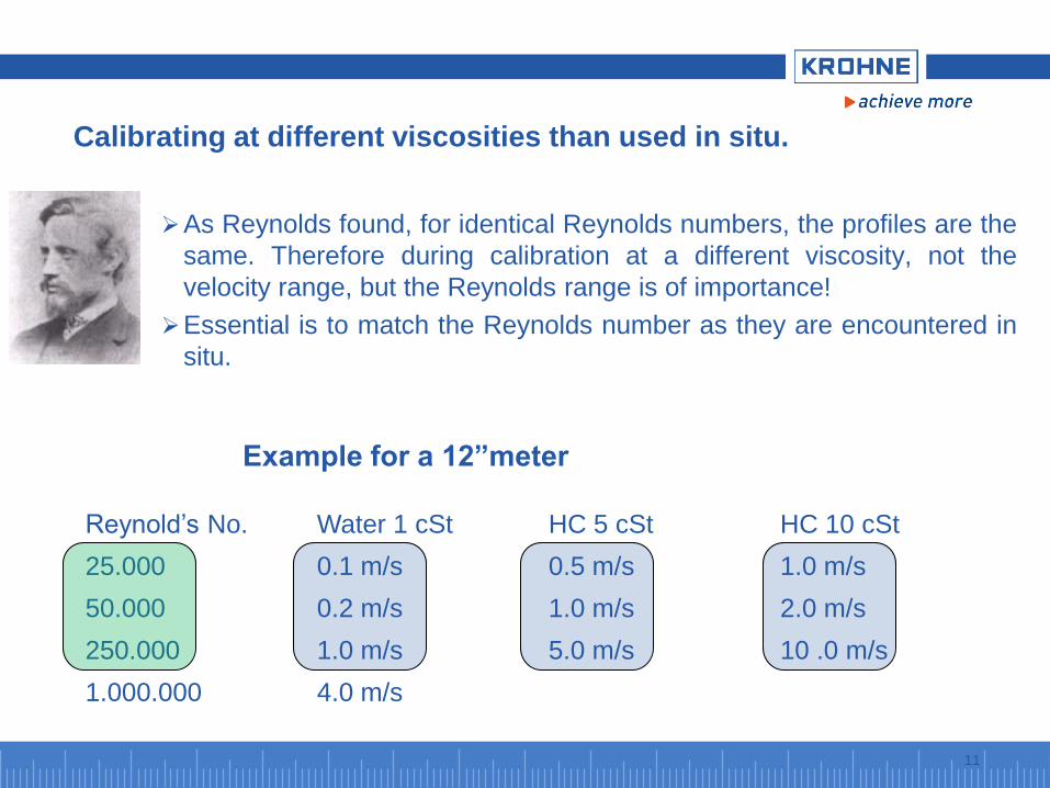
Calibrating at different viscosities than used in situ.
As Reynolds found, for identical Reynolds numbers, the profiles are the
same. Therefore during calibration at a different viscosity, not the
velocity range, but the Reynolds range is of importance!
Essential is to match the Reynolds number as they are encountered in
situ.
Reynold’s No. Water 1 cSt HC 5 cSt HC 10 cSt
25.000 0.1 m/s 0.5 m/s 1.0 m/s
50.000 0.2 m/s 1.0 m/s 2.0 m/s
250.000 1.0 m/s 5.0 m/s 10 .0 m/s
1.000.000 4.0 m/s
Example for a 12”meter
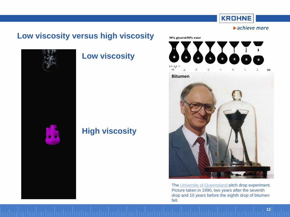
Low viscosity versus high viscosity
12
Low viscosity
High viscosity
The University of Queensland pitch drop experiment.
Picture taken in 1990, two years after the seventh
drop and 10 years before the eighth drop of bitumen
fell.
Bitumen
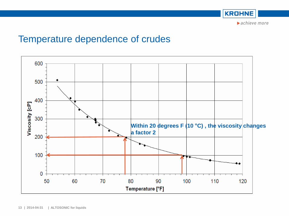
Temperature dependence of crudes
| 2014-04-31 13 | ALTOSONIC for liquids
Within 20 degrees F (10 °C) , the viscosity changes
a factor 2
14
Impact of temperature
Especially highly viscous crude oils are transferred at high
temperatures; therefore temperature fluctuations are commonplace.
As a direct consequence of these temperature variations, large
variations in viscosity occur and as a result of that the flow velocity
profile will change constantly.
So at high viscosities, temperature stability is essential to get an
accurate measurement result.
At low viscosities, there is more turbulent mixing and temperatures play
a smaller role; but than installation effects are more apparent.
15
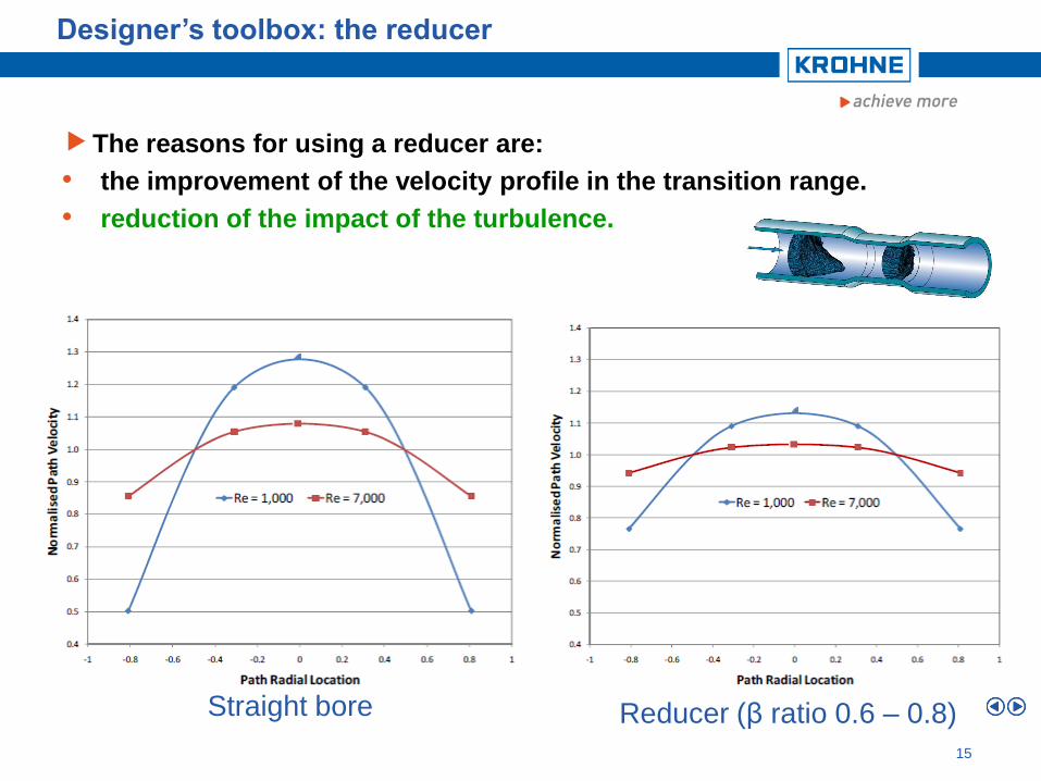
The reasons for using a reducer are:
• the improvement of the velocity profile in the transition range.
• reduction of the impact of the turbulence.
Designer’s toolbox: the reducer
Straight bore Reducer (β ratio 0.6 – 0.8)
Meter design
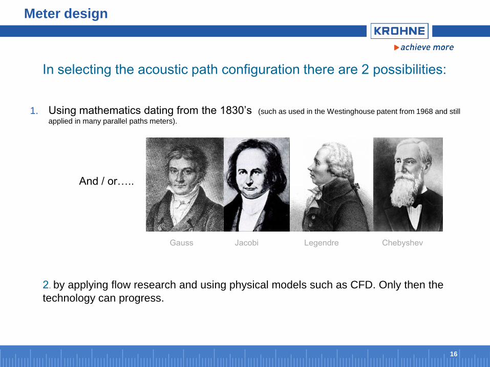
1. Using mathematics dating from the 1830’s (such as used in the Westinghouse patent from 1968 and still
applied in many parallel paths meters).
And / or…..
16
Gauss Jacobi Legendre Chebyshev
In selecting the acoustic path configuration there are 2 possibilities:
2. by applying flow research and using physical models such as CFD. Only then the
technology can progress.
17
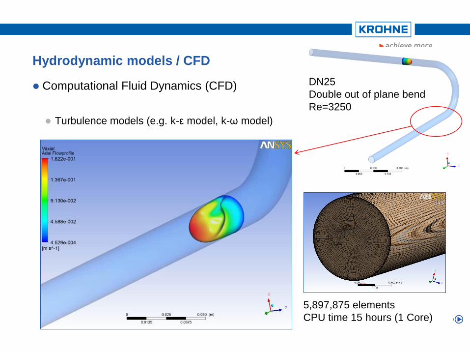
Hydrodynamic models / CFD
Computational Fluid Dynamics (CFD)
Turbulence models (e.g. k-ε model, k-ω model)
5,897,875 elements
CPU time 15 hours (1 Core)
DN25
Double out of plane bend
Re=3250
18
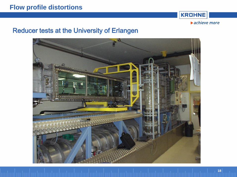
Flow profile distortions
Reducer tests at the University of Erlangen
19
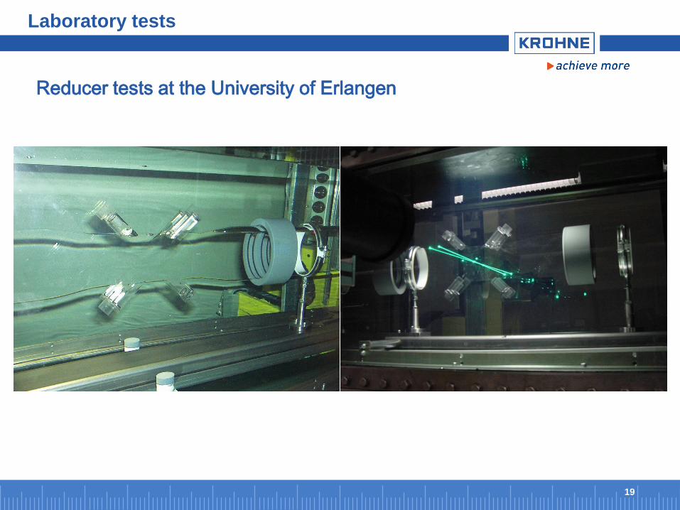
Laboratory tests
Reducer tests at the University of Erlangen
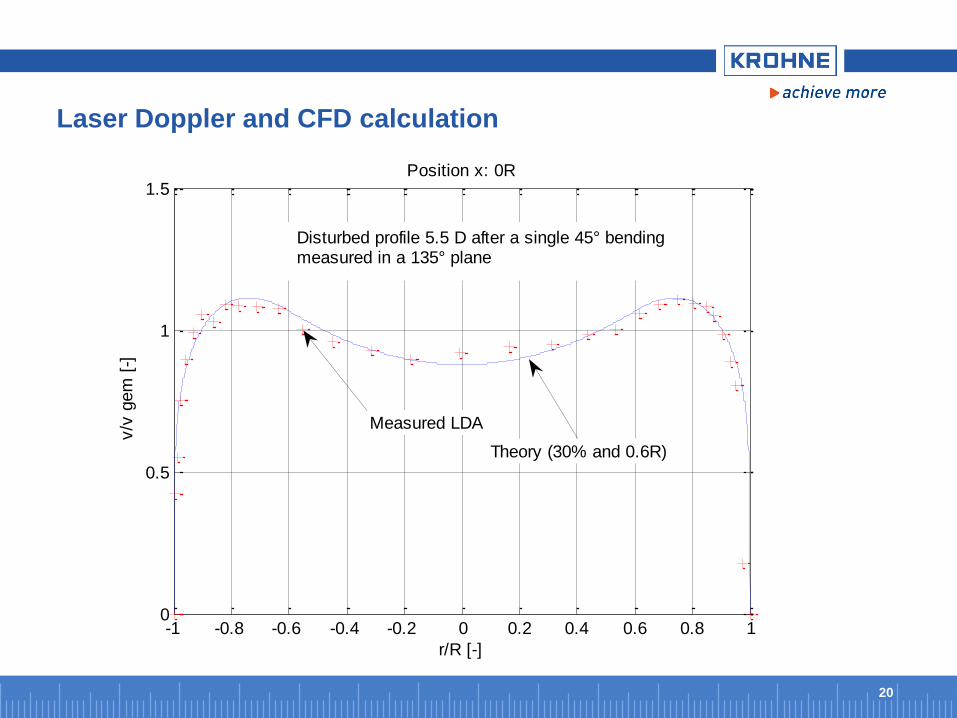
Laser Doppler and CFD calculation
20
-1 -0.8 -0.6 -0.4 -0.2 0 0.2 0.4 0.6 0.8 10
0.5
1
1.5
r/R [-]
v/v
gem
[-]
Position x: 0R
Disturbed profile 5.5 D after a single 45° bendingmeasured in a 135° plane
Measured LDA
Theory (30% and 0.6R)
21
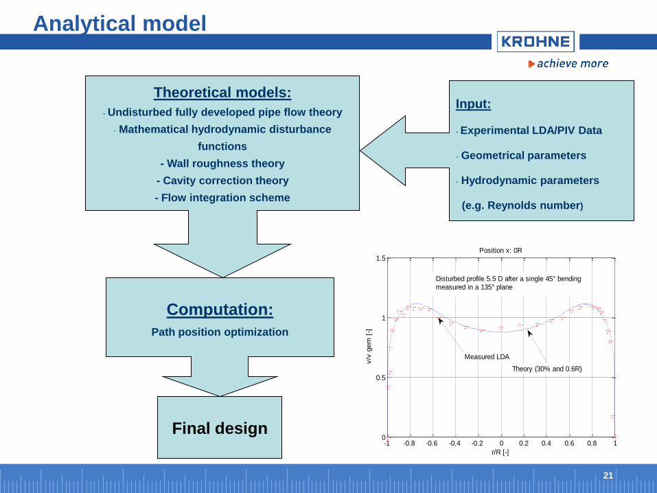
Analytical model
Theoretical models:
- Undisturbed fully developed pipe flow theory
- Mathematical hydrodynamic disturbance
functions
- Wall roughness theory
- Cavity correction theory
- Flow integration scheme
Input:
- Experimental LDA/PIV Data
- Geometrical parameters
- Hydrodynamic parameters
(e.g. Reynolds number)
Computation:
Path position optimization
Final design -1 -0.8 -0.6 -0.4 -0.2 0 0.2 0.4 0.6 0.8 1
0
0.5
1
1.5
r/R [-]
v/v
gem
[-]
Position x: 0R
Disturbed profile 5.5 D after a single 45° bendingmeasured in a 135° plane
Measured LDA
Theory (30% and 0.6R)
22
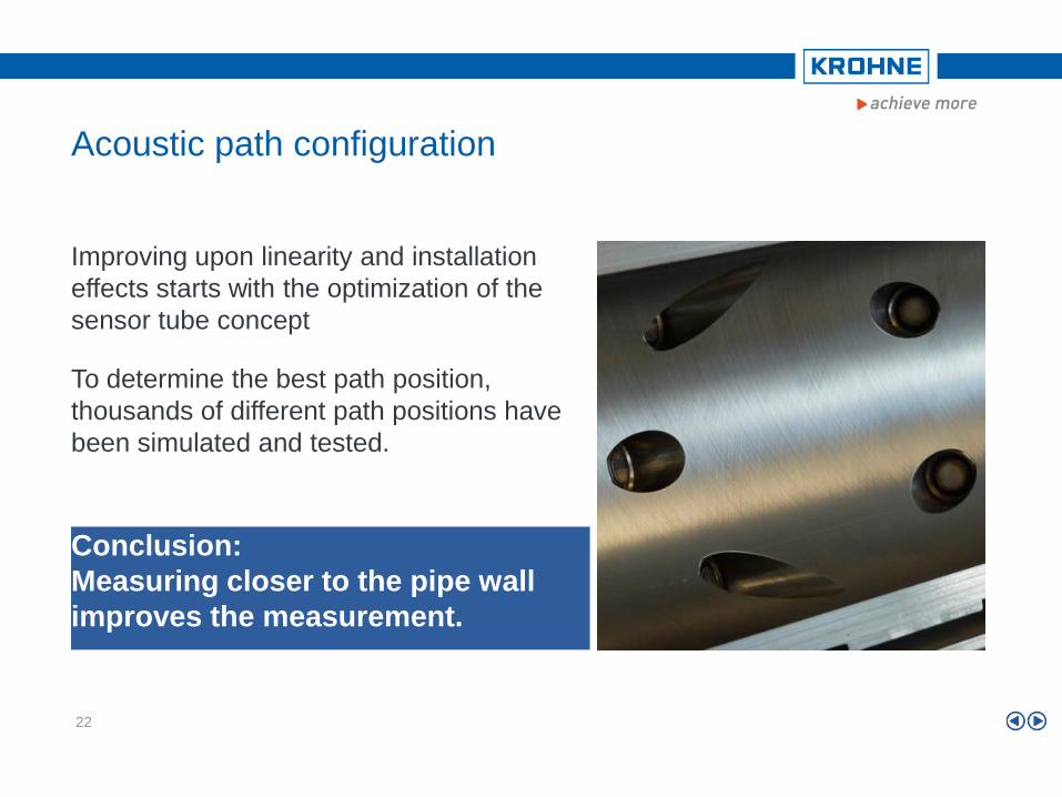
Acoustic path configuration
Improving upon linearity and installation
effects starts with the optimization of the
sensor tube concept
To determine the best path position,
thousands of different path positions have
been simulated and tested.
Conclusion:
Measuring closer to the pipe wall
improves the measurement.
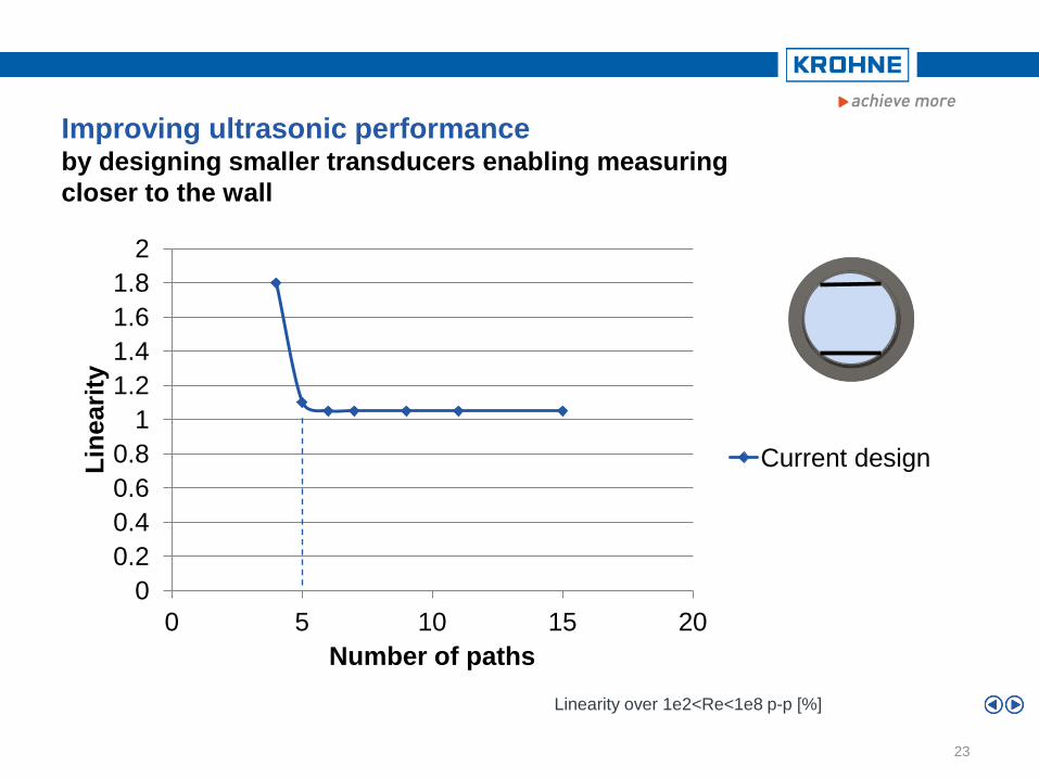
Improving ultrasonic performance by designing smaller transducers enabling measuring
closer to the wall
23
0
0.2
0.4
0.6
0.8
1
1.2
1.4
1.6
1.8
2
0 5 10 15 20
Lin
eari
ty
Number of paths
Current design
Linearity over 1e2<Re<1e8 p-p [%]
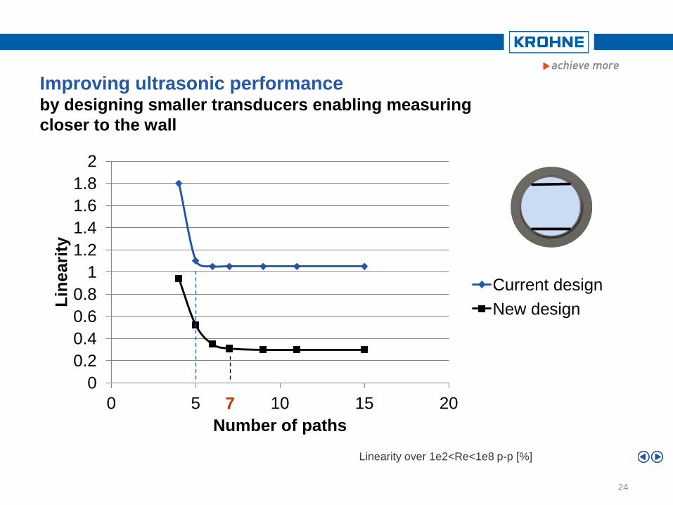
Improving ultrasonic performance by designing smaller transducers enabling measuring
closer to the wall
24
0
0.2
0.4
0.6
0.8
1
1.2
1.4
1.6
1.8
2
0 5 10 15 20
Lin
eari
ty
Number of paths
Current design
New design
Linearity over 1e2<Re<1e8 p-p [%]
7
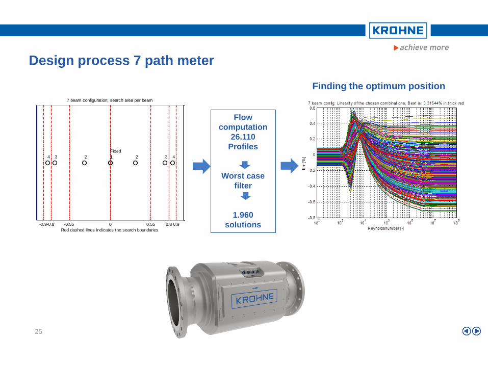
Design process 7 path meter
25
-0.9-0.8 -0.55 0 0.55 0.8 0.9
7 beam configuration; search area per beam
Red dashed lines indicates the search boundaries
Fixed
11 22 33 44
Flow
computation
26.110
Profiles
Worst case
filter
1.960
solutions
Finding the optimum position
25
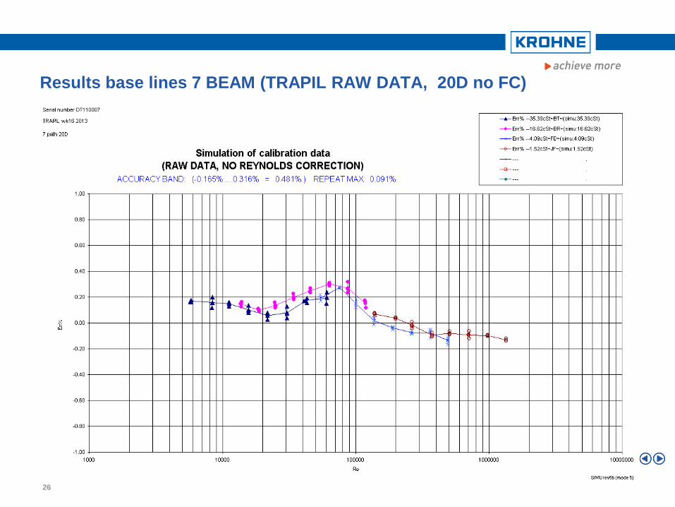
Results base lines 7 BEAM (TRAPIL RAW DATA, 20D no FC)
26
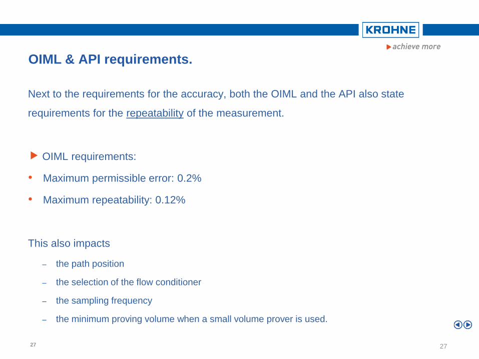
OIML & API requirements.
Next to the requirements for the accuracy, both the OIML and the API also state
requirements for the repeatability of the measurement.
OIML requirements:
• Maximum permissible error: 0.2%
• Maximum repeatability: 0.12%
This also impacts
‒ the path position
‒ the selection of the flow conditioner
‒ the sampling frequency
‒ the minimum proving volume when a small volume prover is used.
27 27
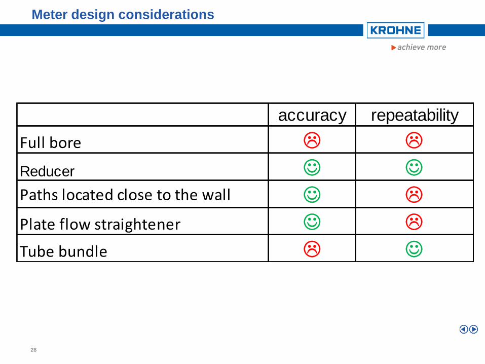
Meter design considerations
28
accuracy repeatability
Full bore L L
Reducer J J
Paths located close to the wall J L
Plate flow straightener J L
Tube bundle L J
28
Meter design conclusions:
The bore reduction has a dominant effect on the meter performance.
The best design, accuracy wise, is a meter with:
A reduced bore
Acoustic paths close to the wall
A plate flow conditioner
Therefore that design is used for the full range Altosonic 5.
29 29
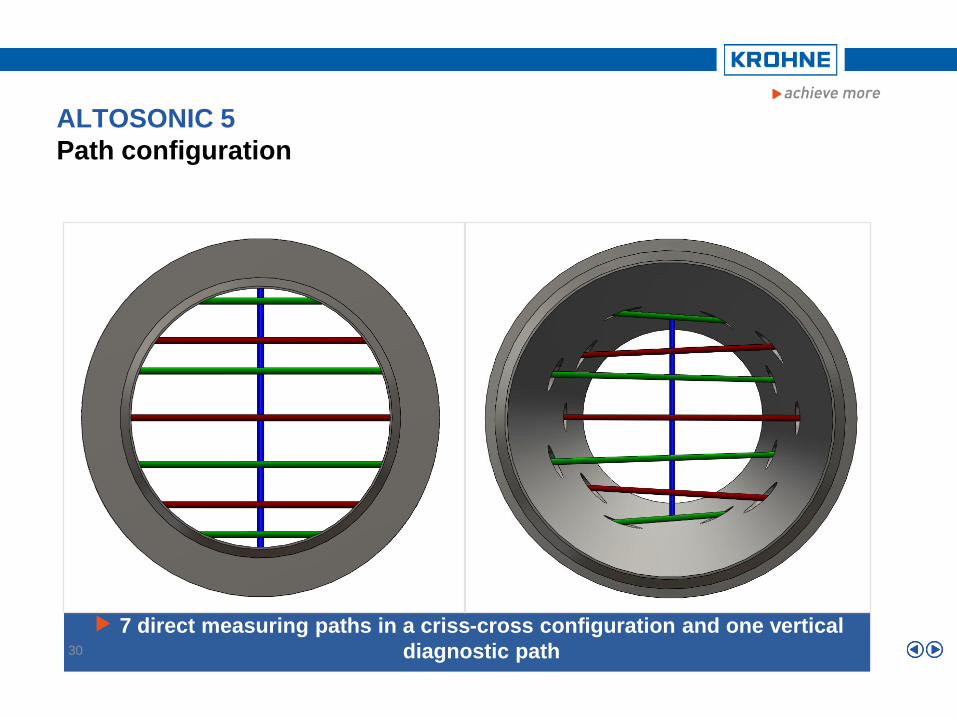
ALTOSONIC 5
Path configuration
7 direct measuring paths in a criss-cross configuration and one vertical
diagnostic path 30
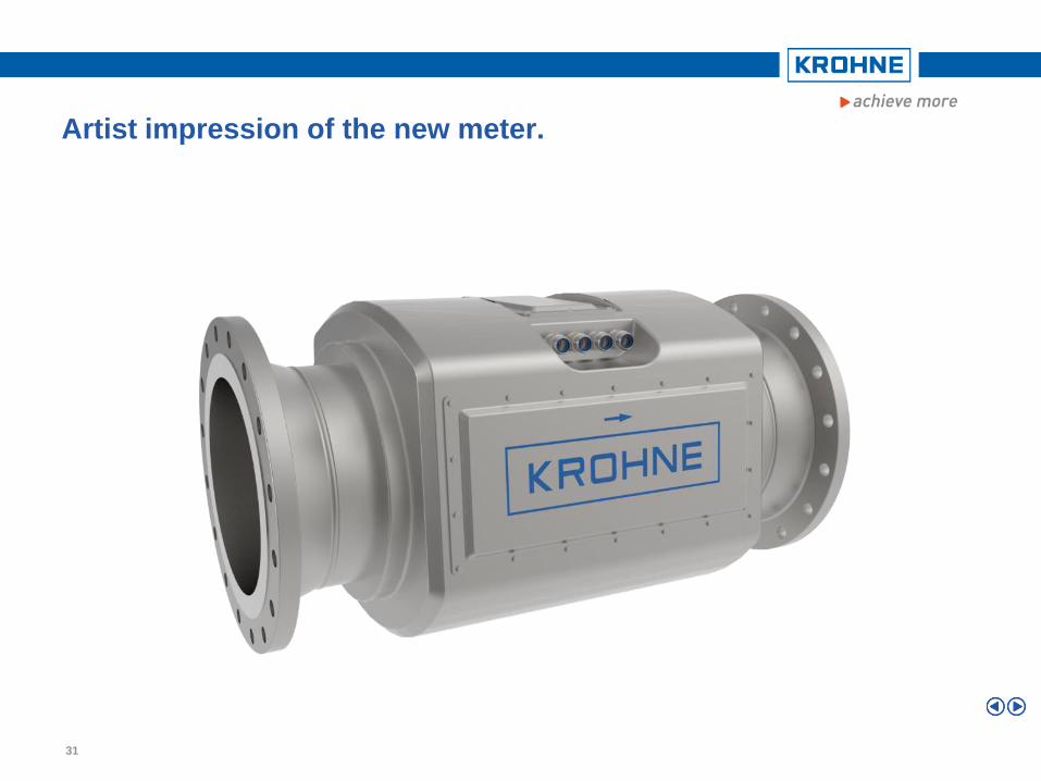
Artist impression of the new meter.
31 31
Jan G. Drenthen &
Pico Brand
1. Introduction
2. Development of the ALTOSONIC 5
3. Test results
• Installation effects
4. Conclusions
Installation tests
The goal for these tests was to quantify the impact of the installation effects
that occur in measuring low viscosity fluids ~ 1cSt.
At much higher viscosities these effects disappear.
The results shown are therefore only valid for low viscosities.
33
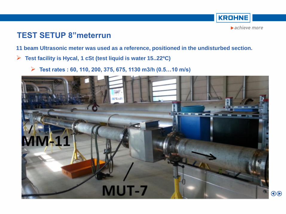
TEST SETUP 8”meterrun
11 beam Ultrasonic meter was used as a reference, positioned in the undisturbed section.
Test facility is Hycal, 1 cSt (test liquid is water 15..22ºC)
Test rates : 60, 110, 200, 375, 675, 1130 m3/h (0.5…10 m/s)
5 repeats per rate, 1 repeat is 100 seconds
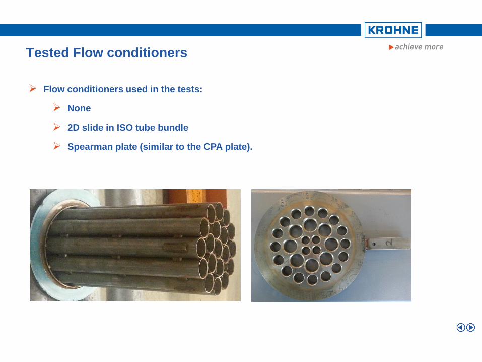
Tested Flow conditioners
35
Flow conditioners used in the tests:
None
2D slide in ISO tube bundle
Spearman plate (similar to the CPA plate).
36
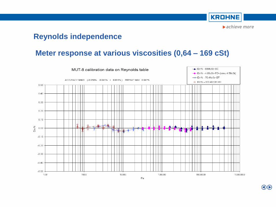
Reynolds independence
Meter response at various viscosities (0,64 – 169 cSt)
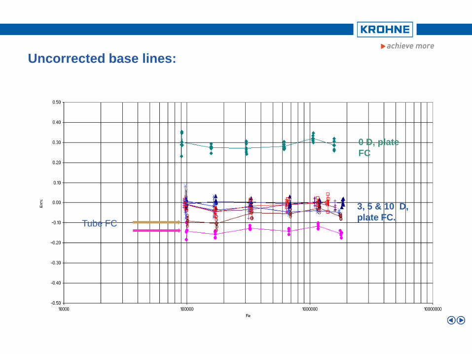
Uncorrected base lines:
0 D
3, 5 & 10 D
Tube FC
Tube FC
0 D, plate
FC
3, 5 & 10 D,
plate FC.
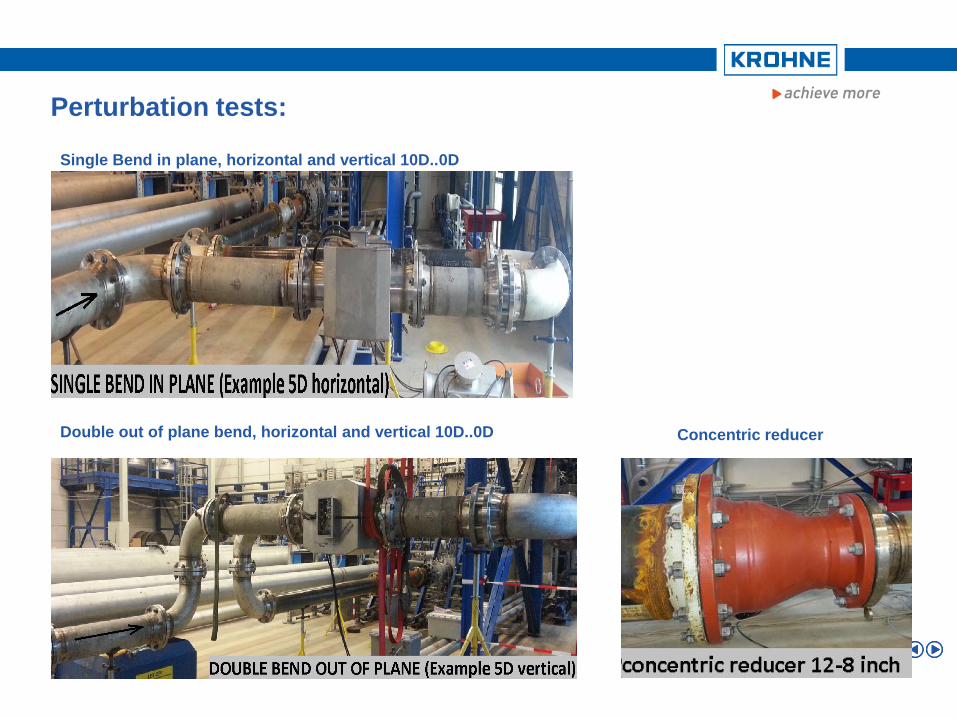
Perturbation tests:
Single Bend in plane, horizontal and vertical 10D..0D
Double out of plane bend, horizontal and vertical 10D..0D Concentric reducer
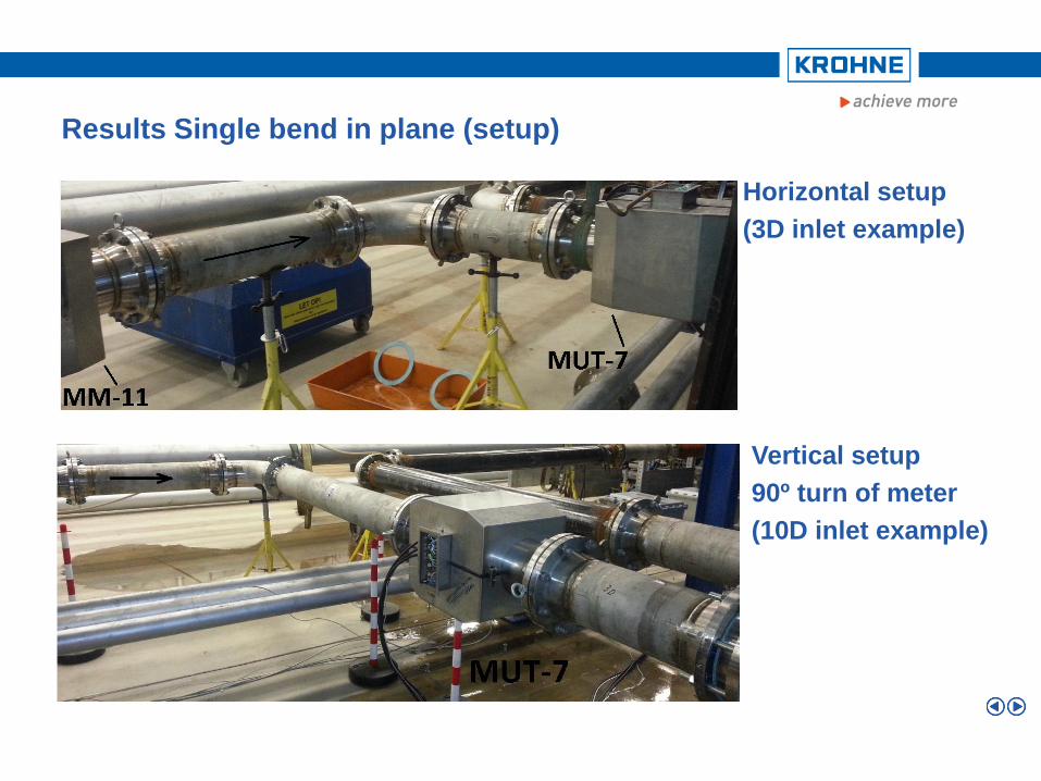
Results Single bend in plane (setup)
Horizontal setup
(3D inlet example)
Vertical setup
90º turn of meter
(10D inlet example)
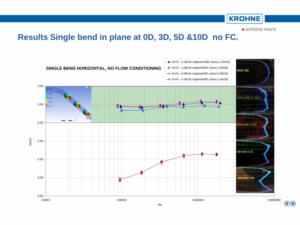
Results Single bend in plane at 0D, 3D, 5D &10D no FC.
SINGLE BEND HORIZONTAL, NO FLOW CONDITIONING
-2.50
-2.00
-1.50
-1.00
-0.50
0.00
0.50
10000 100000 1000000 10000000
Re
Dev%
Err% --1.03cSt~inplaneH10D~(simu:1.03cSt)
Err% --1.08cSt~inplaneH5D~(simu:1.08cSt)
Err% --0.98cSt~inplaneH3D~(simu:0.98cSt)
Err% --1.04cSt~inplaneH0D~(simu:1.04cSt)
SIMU rev5b (mode VISCO) Dev.Inp: 0.00[%]
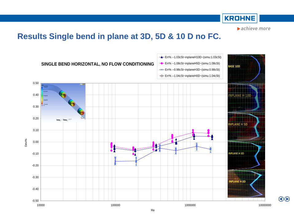
Results Single bend in plane at 3D, 5D & 10 D no FC.
SINGLE BEND HORIZONTAL, NO FLOW CONDITIONING
-0.50
-0.40
-0.30
-0.20
-0.10
0.00
0.10
0.20
0.30
0.40
0.50
10000 100000 1000000 10000000
Re
Dev%
Err% --1.03cSt~inplaneH10D~(simu:1.03cSt)
Err% --1.08cSt~inplaneH5D~(simu:1.08cSt)
Err% --0.98cSt~inplaneH3D~(simu:0.98cSt)
Err% --1.04cSt~inplaneH0D~(simu:1.04cSt)
SIMU rev5b (mode VISCO) Dev.Inp: 0.00[%]
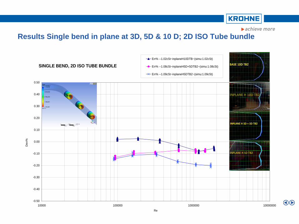
Results Single bend in plane at 3D, 5D & 10 D; 2D ISO Tube bundle
SINGLE BEND, 2D ISO TUBE BUNDLE
-0.50
-0.40
-0.30
-0.20
-0.10
0.00
0.10
0.20
0.30
0.40
0.50
10000 100000 1000000 10000000
Re
Dev%
Err% --1.02cSt~inplaneH10DTB~(simu:1.02cSt)
Err% --1.08cSt~inplaneH5D+5DTB2~(simu:1.08cSt)
Err% --1.09cSt~inplaneH5DTB2~(simu:1.09cSt)
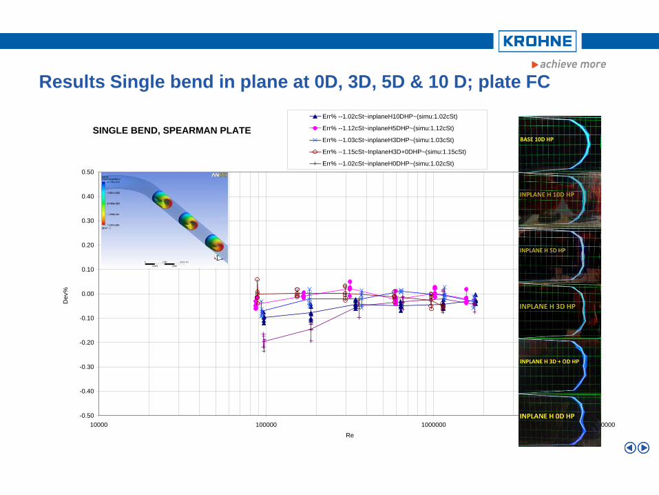
Results Single bend in plane at 0D, 3D, 5D & 10 D; plate FC
SINGLE BEND, SPEARMAN PLATE
-0.50
-0.40
-0.30
-0.20
-0.10
0.00
0.10
0.20
0.30
0.40
0.50
10000 100000 1000000 10000000
Re
Dev%
Err% --1.02cSt~inplaneH10DHP~(simu:1.02cSt)
Err% --1.12cSt~inplaneH5DHP~(simu:1.12cSt)
Err% --1.03cSt~inplaneH3DHP~(simu:1.03cSt)
Err% --1.15cSt~InplaneH3D+0DHP~(simu:1.15cSt)
Err% --1.02cSt~inplaneH0DHP~(simu:1.02cSt)
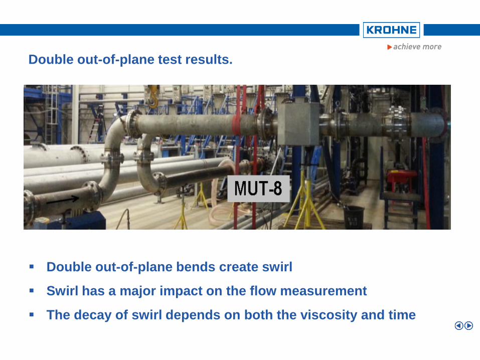
Double out-of-plane test results.
Double out-of-plane bends create swirl
Swirl has a major impact on the flow measurement
The decay of swirl depends on both the viscosity and time
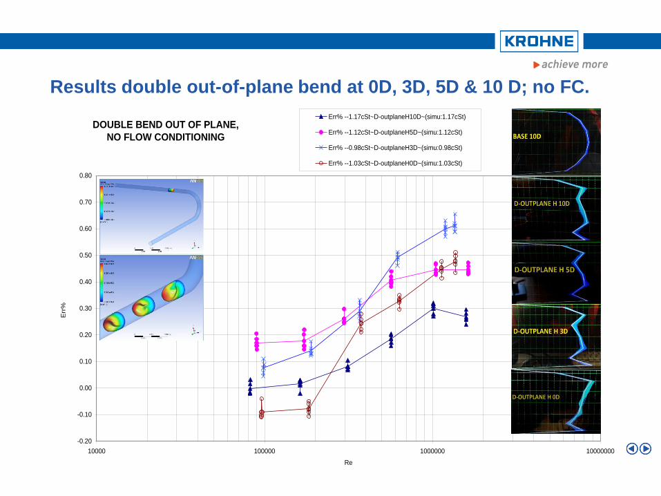
Results double out-of-plane bend at 0D, 3D, 5D & 10 D; no FC.
DOUBLE BEND OUT OF PLANE,
NO FLOW CONDITIONING
-0.20
-0.10
0.00
0.10
0.20
0.30
0.40
0.50
0.60
0.70
0.80
10000 100000 1000000 10000000
Re
Err
%
Err% --1.17cSt~D-outplaneH10D~(simu:1.17cSt)
Err% --1.12cSt~D-outplaneH5D~(simu:1.12cSt)
Err% --0.98cSt~D-outplaneH3D~(simu:0.98cSt)
Err% --1.03cSt~D-outplaneH0D~(simu:1.03cSt)
SIMU rev5b (mode VISCO) Dev.Inp: 0.00[%]
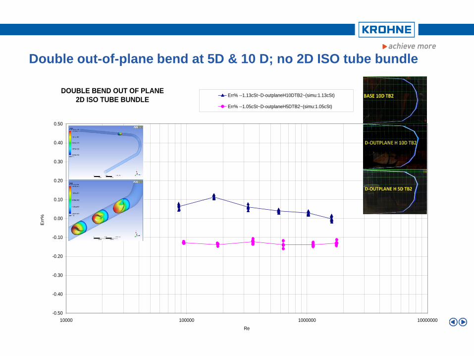
Double out-of-plane bend at 5D & 10 D; no 2D ISO tube bundle
DOUBLE BEND OUT OF PLANE
2D ISO TUBE BUNDLE
-0.50
-0.40
-0.30
-0.20
-0.10
0.00
0.10
0.20
0.30
0.40
0.50
10000 100000 1000000 10000000
Re
Err
%
Err% --1.13cSt~D-outplaneH10DTB2~(simu:1.13cSt)
Err% --1.05cSt~D-outplaneH5DTB2~(simu:1.05cSt)
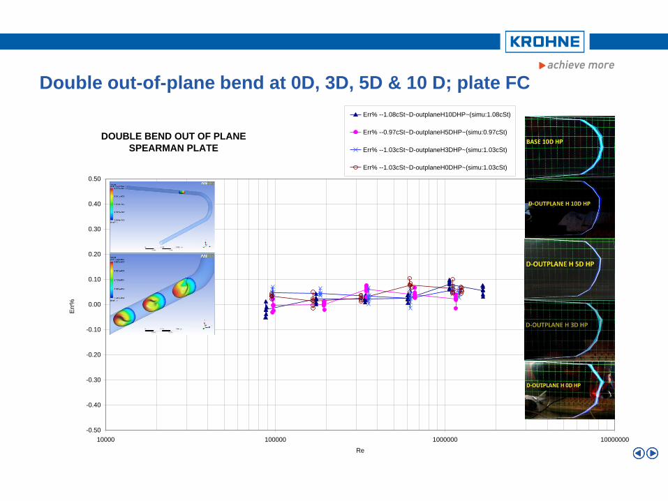
Double out-of-plane bend at 0D, 3D, 5D & 10 D; plate FC
DOUBLE BEND OUT OF PLANE
SPEARMAN PLATE
-0.50
-0.40
-0.30
-0.20
-0.10
0.00
0.10
0.20
0.30
0.40
0.50
10000 100000 1000000 10000000
Re
Err
%
Err% --1.08cSt~D-outplaneH10DHP~(simu:1.08cSt)
Err% --0.97cSt~D-outplaneH5DHP~(simu:0.97cSt)
Err% --1.03cSt~D-outplaneH3DHP~(simu:1.03cSt)
Err% --1.03cSt~D-outplaneH0DHP~(simu:1.03cSt)
Jan G. Drenthen &
Pico Brand
1. Introduction
2. Development of the ALTOSONIC 5
3. Test results
• Installation effects
• Meter proving
4. Conclusions
The API Ch 5.8 is based on turbine meters.
Turbine meters average the flow over the length of the rotor blade section and
are not capable to measure high frequency fluctuations. Ultrasonic meters detect
all these natural occurring fluctuations in the flow. Hence the output of ultrasonic
meters possess a much larger scatter than turbine meters.
To reduce the scatter to the level of the turbine meter, the ultrasonic meter must
average over a larger time/volume.
Proving according to API Ch 5.8
Proving ultrasonic meters with a SVP is not easy!
49
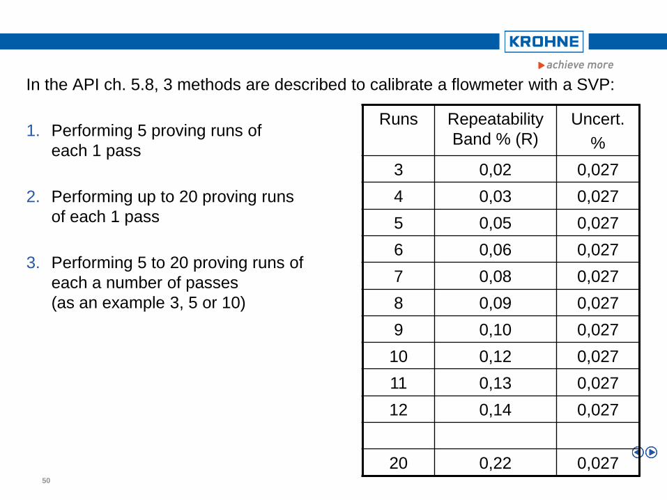
Runs Repeatability
Band % (R)
Uncert.
%
3 0,02 0,027
4 0,03 0,027
5 0,05 0,027
6 0,06 0,027
7 0,08 0,027
8 0,09 0,027
9 0,10 0,027
10 0,12 0,027
11 0,13 0,027
12 0,14 0,027
20 0,22 0,027
In the API ch. 5.8, 3 methods are described to calibrate a flowmeter with a SVP:
1. Performing 5 proving runs of
each 1 pass
2. Performing up to 20 proving runs
of each 1 pass
3. Performing 5 to 20 proving runs of
each a number of passes
(as an example 3, 5 or 10)
50
Minimum proving volume
The minimum proving volume is a function of:
The meter size.
The flow regime (laminar – transition – turbulent).
The turbulence level.
The number of acoustic paths.
The sampling rate.
In the design of the new Altosonic 5, both the number of paths as
well as the sampling rate have been optimized for use with SVP.
51
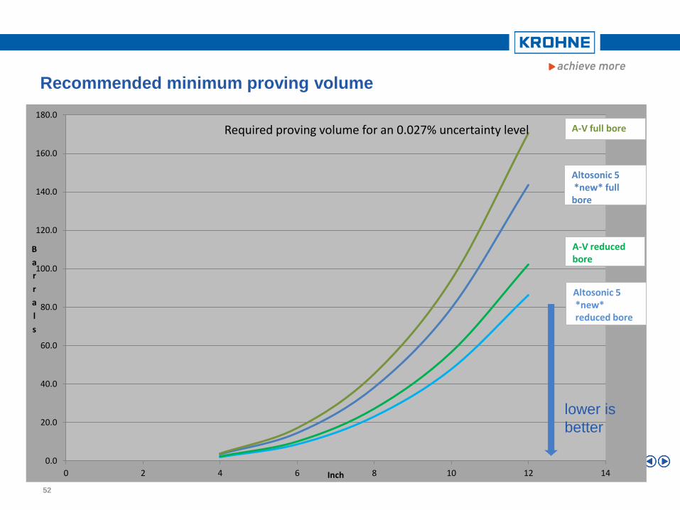
Recommended minimum proving volume
52
0.0
20.0
40.0
60.0
80.0
100.0
120.0
140.0
160.0
180.0
0 2 4 6 8 10 12 14
B
a
r
r
a
l
s
Inch
Required proving volume for an 0.027% uncertainty level A-V full bore
Altosonic 5 *new* full bore
A-V reduced bore
Altosonic 5 *new* reduced bore
52
lower is
better
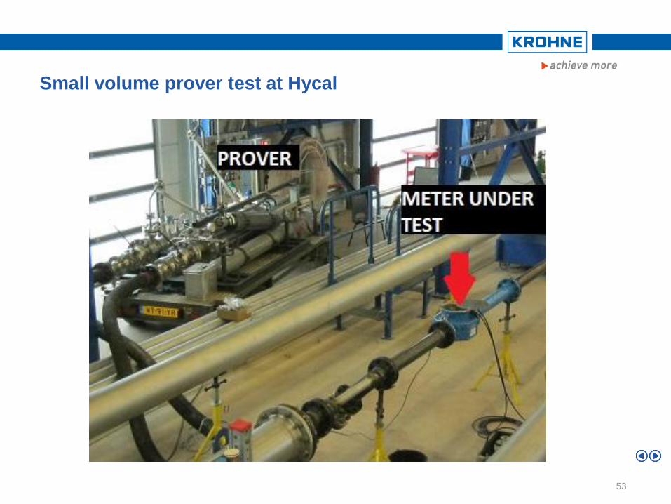
Small volume prover test at Hycal
53
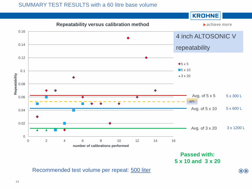
SUMMARY TEST RESULTS with a 60 litre base volume
4 inch ALTOSONIC V
repeatability
0
0.02
0.04
0.06
0.08
0.1
0.12
0.14
0.16
0 2 4 6 8 10 12 14 16
Rep
eata
bilit
y
number of calibrations performed
Repeatability versus calibration method
5 x 5
5 x 10
3 x 20
Avg. of 5 x 5
Avg. of 5 x 10
Avg. of 3 x 20
API
Recommended test volume per repeat: 500 liter
Passed with:
5 x 10 and 3 x 20
54
5 x 300 L
5 x 600 L
3 x 1200 L
SUMMARY TEST RESULTS with a 60 litre base volume
6 inch ALTOSONIC V
repeatabilities
0
0.02
0.04
0.06
0.08
0.1
0.12
0.14
0 1 2 3 4 5 6 7 8
Rep
eata
bilit
y
number of calibrations performed
Repeatability versus calibration method
5 x 5
5 x 10
3 x 20
5 x 5
5 x 10
3 x 20
Recommended test volume per repeat: 1900 liter
All tests failed!
Too small test volume!
55
5 x 300 L
5 x 600 L
3 x 1200 L
API
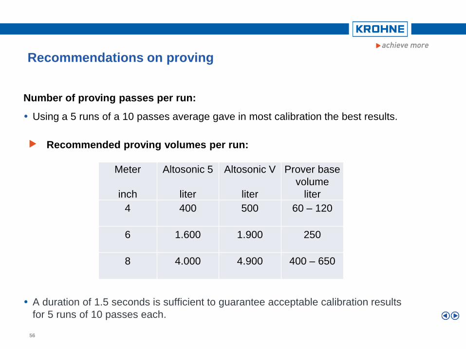
Recommendations on proving
Meter
inch
Altosonic 5
liter
Altosonic V
liter
Prover base
volume
liter
4
400
500
60 – 120
6
1.600
1.900
250
8
4.000
4.900
400 – 650
Recommended proving volumes per run:
Number of proving passes per run:
Using a 5 runs of a 10 passes average gave in most calibration the best results.
A duration of 1.5 seconds is sufficient to guarantee acceptable calibration results
for 5 runs of 10 passes each.
56
Jan G. Drenthen &
Pico Brand
1. Introduction
2. Development of the ALTOSONIC 5
3. Test results
• Installation effects
• Meter proving
4. Conclusions
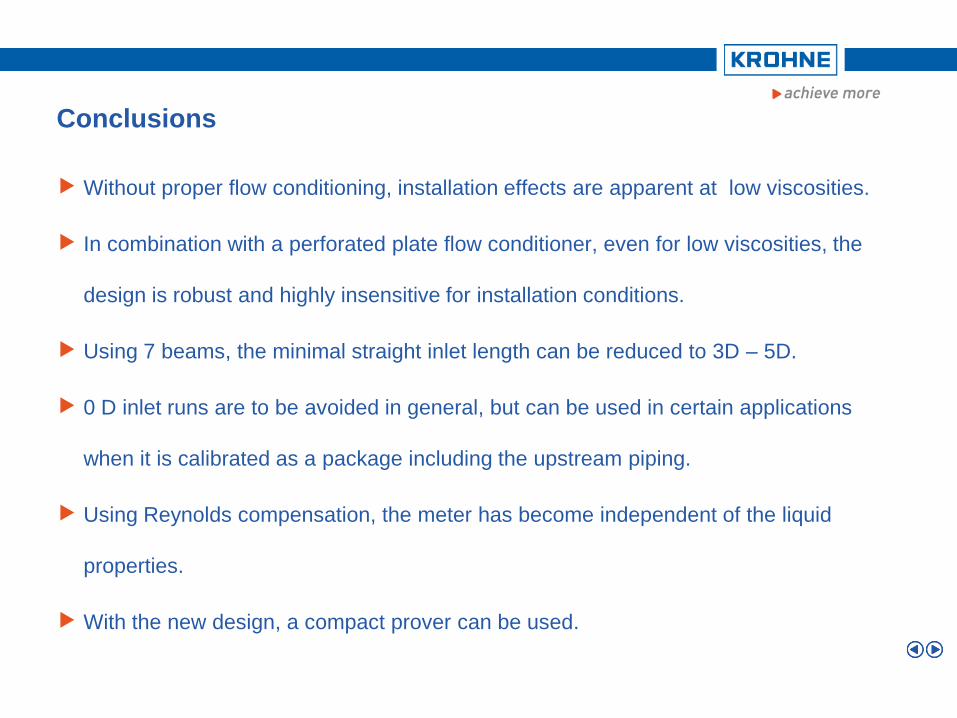
Conclusions
Without proper flow conditioning, installation effects are apparent at low viscosities.
In combination with a perforated plate flow conditioner, even for low viscosities, the
design is robust and highly insensitive for installation conditions.
Using 7 beams, the minimal straight inlet length can be reduced to 3D – 5D.
0 D inlet runs are to be avoided in general, but can be used in certain applications
when it is calibrated as a package including the upstream piping.
Using Reynolds compensation, the meter has become independent of the liquid
properties.
With the new design, a compact prover can be used.
58
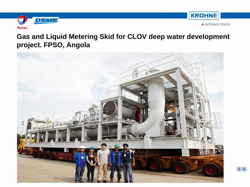
Gas and Liquid Metering Skid for CLOV deep water development
project. FPSO, Angola
| Major Projects Reference Overview

The King is dead…….
60
.. long live the new King
61

62
Any Questions?

63
In for a bite?
Jan G. Drenthen &
Pico Brand
Thank you for your attention!