LUND UNIVERSITY

PO Box 117221 00 Lund+46 46-222 00 00

Initial Characterization of Massive Multi-User MIMO Channels at 2.6 GHz in Indoor andOutdoor Environments

Flordelis, Jose; Gao, Xiang; Dahman, Ghassan; Tufvesson, Fredrik; Edfors, Ove

2015

Link to publication

Citation for published version (APA):Flordelis, J., Gao, X., Dahman, G., Tufvesson, F., & Edfors, O. (2015). Initial Characterization of Massive Multi-User MIMO Channels at 2.6 GHz in Indoor and Outdoor Environments. Paper presented at JointNEWCOM/COST Workshop on Wireless Communications (JNCW), Barcelona, Spain.

General rightsCopyright and moral rights for the publications made accessible in the public portal are retained by the authorsand/or other copyright owners and it is a condition of accessing publications that users recognise and abide by thelegal requirements associated with these rights.

• Users may download and print one copy of any publication from the public portal for the purpose of private studyor research. • You may not further distribute the material or use it for any profit-making activity or commercial gain • You may freely distribute the URL identifying the publication in the public portalTake down policyIf you believe that this document breaches copyright please contact us providing details, and we will removeaccess to the work immediately and investigate your claim.

EUROPEAN COOPERATIONIN THE FIELD OF SCIENTIFICAND TECHNICAL RESEARCH

————————————————EURO-COST

————————————————

IC1004 TD(15)W1023Barcelona, SpainOctober 14–15, 2015

SOURCE: EIT, Dept. of Electrical and Information Technology,Lund University,Sweden

Initial Characterization of Massive Multi-User MIMO Channels at 2.6 GHzin Indoor and Outdoor Environments

Jose Flordelis, Xiang Gao, Ghassan Dahman, Ove Edfors and Fredrik TufvessonDept. of Electrical and Information TechnologyLund UniversityBox 118SE-221 00 LundSWEDENPhone: +46 46 2229179Fax: +46 46 129948Email: firstname.lastname@eit.lth.se

Initial Characterization of Massive Multi-UserMIMO Channels at 2.6 GHz in Indoor and

Outdoor Environments

Jose Flordelis, Xiang Gao, Ghassan Dahman, Ove Edfors and Fredrik Tufvesson

Dept. of Electrical and Information Technology, Lund University, Lund, SwedenEmail: firstname.lastname@eit.lth.se

Abstract—The channel properties have a large influ-ence on user separability in massive multi-user multiple-input multiple-output (massive MIMO) systems. In thispaper we present spatio-temporal characteristics obtainedfrom massive MIMO channel measurements at 2.6 GHz.The results are based on data acquired in both indoorand outdoor scenarios where a base station (BS) equippedwith 64 dual-polarized antenna elements communicatessimultaneously with nine single-antenna users. In theoutdoor scenarios the BS is placed at two rooftops withdifferent heights and the users are confined to a five-meter diameter circle and move randomly at pedestrianspeeds. In the indoor scenarios, the users are locatedclose to each other in a lecture theater and the BSis placed at various locations in the room. We reporton the observed distribution of the delay spreads andangular spreads. Furthermore, the multi-user performancein terms of singular value spread of the MU-MIMOchannel is also reported. Finally, statistics of the coherencetime and coherence bandwidth of the propagation channelin various scenarios are given. The results are importantfor the design and analysis of massive MIMO systems,as well as in the development of realistic massive MIMOchannel models.

Keywords—multi-user multiple-input multiple-outputsystems, MU-MIMO, massive MIMO, large-scale MIMO,MIMO channel measurements, spatial separation, time evo-lution, channel model, second-order moment.

I. INTRODUCTION

Massive MIMO is an emerging communication tech-nology promising order-of-magnitude improvements indata throughput, link reliability, range, and transmit-energy efficiency [1]–[4]. These benefits arise fromleveraging the additional degrees of freedom providedby an excess of antenna elements at the BS side.A typical massive MIMO system can consist of oneor more BSs equipped with many, M = 100, say,antenna elements serving K single-antenna users in thesame time-frequency resource. K is in the order of10 to 20 users, possibly more. Due to its potential togreatly increase spectral efficiency compared to today’ssystems, massive MIMO is considered as one of the

main directions towards future 5G communication sys-tems [5]–[7].

Several measurement campaigns have been con-ducted to study the performance of massive MIMOin real propagation environments. In [8]–[10], we re-ported outdoor massive MIMO channel measurementsat 2.6 GHz with a linear array and a cylindrical array,both having 128 antenna elements. The investigationsconcluded that real propagation channels allow effectiveuse of massive MIMO technology in the sense thata large fraction of the sum-rate capacity of MIMOchannels with independent and identically distributed(i.i.d.) Rayleigh fading can be achieved in real prop-agation channels with linear precoding schemes. Thisis also shown in [11] for indoor BS measurements.In [12] massive MIMO channel measurements using ascalable antenna array consisting of up to 112 elementswere reported. The results in [12] further support theconclusions drawn in [9]–[11] that theoretical gains ofmassive MIMO can be achieved in practice. More recentresults in [13] indicate that the benefits of massiveMIMO can be reaped even in the difficult scenario of agroup of users located close to each other with line-of-sight (LOS) to the BS. Altogether, the combined setof published experimental results on massive MIMOelevates it from a mere theoretical concept to a practicaltechnology.

In this paper we present spatio-temporal character-istics obtained from massive MIMO channel measure-ments at 2.6 GHz in various indoor and outdoor scenar-ios. During the measurements users are distributed withhigh density and located close to each other, possiblywith many other passive users acting as scatterers orshadowing objects. Furthermore, the multi-user perfor-mance in terms of singular value spread of the MU-MIMO channel is also reported. Finally, statistics ofthe coherence time and coherence bandwidth of thepropagation channel in various scenarios are given. Theresults are important for the design and analysis ofmassive MIMO systems, as well as in the developmentof realistic massive MIMO channel models.

II. MEASUREMENT DESCRIPTION

This section provides an overview of the scenarioschosen for the massive MIMO measurement campaigns,a description of the actual measurement environmentsand a short account of the measurement equipment.

A. Measurement Scenarios

In this work we consider two system scenariosidentified in [14] as important for future 5G systems,namely “open exhibition” and “crowded auditorium”.The main characteristics of these two scenarios aresummarized in Tab. I and Tab. II (taken from [15]),respectively.

According to [14], open exhibition consists ofoutdoor-deployed (macro) BSs serving outdoor-locatedUEs. UEs are distributed randomly with high densityand move at pedestrian speeds. UEs locations are inprinciple completely random, although some correlationmay exist for both the UEs positions and the trafficpatterns at specific times and/or locations.

One of the most important aspects to analyze andmodel is the user separability of closely spaced users,possibly with many other (passive) people being aroundacting as scatterers or shadowing objects and thusinteracting with the nearby MS antenna. In this scenarioit is important to include the effect of the user hand, theuser body and the user antenna.

TABLE I. “OPEN EXHIBITION” MAIN CHARACTERISTICS. [15]

Parameter ValuePropagation environment OutdoorCell geometry / Size Irregular, delimited geometry / Medium to

largeUE distribution Random, but clustered, with high densityUE speed Up to 7 km/hLOS/NLOS BothShadow fading PresentChannel model COST2100METIS relation TC9 “Open air festival”Examples Outdoor conference center, crowded square

TABLE II. “CROWDED AUDITORIUM” MAINCHARACTERISTICS. [15]

Parameter ValuePropagation environment IndoorCell geometry and size Determined by scenario boundariesUE distribution Random, but clustered, with high densityUE speed Mostly static, up to 3 km/hLOS/NLOS BothShadow fading Not presentChannel model COST2100Examples Indoor conference center, office, concert hall,

indoor arenaMETIS relation TC1: “Virtual reality office”, TC3 “Shopping

mall”, TC4: “Stadium”

From a measurement perspective, while still cap-turing the essential characteristics of the channel, wedownscale the scenario to a group of a few users beinglocated close to each other, with or without other peoplearound, simultaneously communicating with a macro

BS in LOS or NLOS. In our measurements we have 9single-antenna users confined to a circle of 5 m diameterand describing random trajectories at pedestrian speedswhile holding the MS in browse mode in front of theirbody with one hand. We consider two different positionsof the BS, high- and low-roof, and several positionsof the UE circle (UE sites), in both LOS and NLOSto the BS. The main characteristics of the outdoormeasurement scenarios are summarized in Tab. III.

Crowded auditorium provides the indoor counterpartof the outdoor scenario described above. In this scenarioboth UEs and BSs are, respectively, located and de-ployed indoors. The UEs are randomly distributed withhigh density, possibly with correlated UEs positionsand traffic patterns. The UEs are almost static in mostcases and NLOS propagation conditions are expected. Asubcase may be considered in which the UEs are static,placed at deterministic locations (e.g., seats in a concerthall) and channels contain LOS components.

Again, we capture the essential characteristics ofthis scenario by downscaling it to a case with a groupof closely located indoor users in a lecture theatercommunicating with a BS mostly in LOS but withsome obstructions. The users are seated regularly withand without other passive users around them acting asscatterers or shadowing objects. As opposed to the out-door case we expect larger angular spreads due to moreinteraction with the indoor walls. Users hold the MS inbrowse mode in front of their bodies with one hand, allusers facing the theater stage. Although the positions ofthe users are static, MSs describe random trajectories infront of each user’s body at a speed of one revolutionevery 2 to 4 seconds. The purpose of the MS movementsis to generate statistics of typical movements of MSsin a lecture theater. In our measurements we considerfour BS locations and two different UE sites. The maincharacteristics of the indoor measurement scenarios aresummarized in Tab. IV.

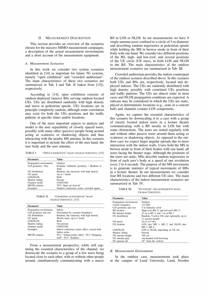
TABLE III. “OUTDOOR” MEASUREMENTS MAINCHARACTERISTICS.

Parameter ValuePropagation environment OutdoorCarrier frequency 2.6 GHzCell geometry and size 5 m diameter circleBS location High-roof (BS 2) and low-roof (BS 1)BS antenna height 23 m at BS 2, and 7 m at BS 1UE distribution Random, 9 active UEs and, optionally, up to

11 passive peopleUE speed Up to 0.5 m/sUE location LOS sites MS 1, MS 2, and NLOS sites

MS 3, MS 4LOS/NLOS LOS or NLOS, depending on UE siteShadow fading PresentUE antenna height 160 cmUE antenna grip one-handed web-browsingUE antenna tilt 45◦ from the vertical

B. Measurement Environment

In the outdoor case, measurements took placeat the campus of Lund University, Lund, Sweden

TABLE IV. “INDOOR” MEASUREMENTS MAINCHARACTERISTICS.

Parameter ValuePropagation environment IndoorCarrier frequency 2.6 GHzUser distribution Located at 4 rows of 5 adjacent seats

(2.5×3.5 m2)BS antenna height 3.2 mUE distribution Deterministic, 9 active UEs and, optionally,

11 passive peopleUE speed UE antennas move in random trajectories in

front of the user at low speedLOS/NLOS LOS with obstructions by room furniture and

users seating nearbyUE antenna height 50 cm to 100 cm over the floor level, occa-

sionally below furniture lineUE antenna grip one-handed web-browsingUE antenna tilt Vertical, 45◦ downtilt

(55.711510 N, 13.210405 E), which can be described asa suburban environment having detached buildings withtwo to five floors and open areas with low vegetationand some trees. Fig. 1 shows an aerial photo of themeasurement area. The BS antenna array was placed onthe roof of the E-building, at two different levels: BS 1on top of a two-floors roof (low-roof) and BS 2 on topof a five-floors roof (high-roof). The precise locationsof BS 1 and BS 2 are given in Fig. 1. Several UEsites, labeled MS 1 to MS 4, were considered, withsites MS 1 and MS 2 having LOS conditions to theBS array, and sites MS 3 through MS 5 having NLOSconditions (see Fig. 1). At each UE site, we have a5 m diameter circle and up to nine users moving insideit, representing a situation of high user density. Duringthe measurements, users were holding the antennasinclining them at about 45◦, so that we have bothvertical and horizontal polarizations reaching the BSantenna array. Note that, since users were allowed toturn around, the LOS component to the BS can beblocked in some snapshots, by the user holding theantenna or by other users (see Fig. 2).

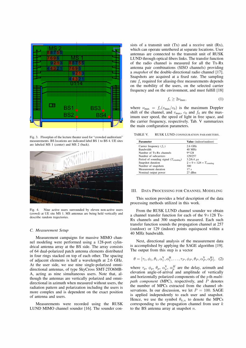
In the indoor case, measurements took place inlecture hall E:A. Lecture hall E:A has a picthed floorso that listeners in the rear are sat higher than thoseat the front and have LOS to the theater stage. Note,however, that handheld devices are typically held at orclose to desk level and, thus, the LOS from the deviceto BS may at times be obstructed by nearby listeners orby room furniture. Fig. 3 shows a floor plan of lecturehall E:A. In the measurements, we consider four BSlocations labeled BS 1 to BS 4, and two UE sites,labeled MS 1 and MS 2. All four BS locations are onthe stage side of the lecture hall, with locations BS 1and BS 2 sideways centered and locations BS 3 andBS 4 next to a corner. We note that, at locations BS 1and BS 3, the BS antenna array is located at least oneRayleigh distance apart from walls and other interactingobjects and, thus, wavefronts impinging on the BS arraycan be assumed plane. On the other hand, at locationsBS 2 and BS 4, the BS antenna array is located nextto one or two walls, as it might be the case in pratical

Fig. 1. Aerial photo of the outdoor measurement area. BS locationsare indicated by labels BS 1 (low-roof) and BS 2 (high-roof). UEsites are labeled with MS 1 to MS 4, and the locations of the 5 mdiameter circles have also been indicated. UE sites MS 1 and MS 2have LOS condition to the BS, while MS 3 and MS 4 have NLOS.

(a) (b)

Fig. 2. (a) A user holding the MS user equipment antenna with aninclination of 45◦. (b) Users moving randomly within the five-meterdiameter circle at UE site MS 4.

BS indoor deployments. In all cases, the antenna arrayhas been placed at a height of 3.2 m from the floor. UEsites MS 1 and MS 2 consist of a regular grid of fourrows with five adjacent seats each, with an approximatearea of 2.5×3.5 m2. Site MS 1 comprises the centerseats, whereas site MS 2 is located at the far cornerfrom BS 3 and BS 4 and, in this sense, represents aworst case location. For each UE site, two differentseat arrangements with nine seats each are considered,as illustrated in Fig. 3, where seats pertaining to eacharrangement have been color-coded in red and blue. Therest of the seats are possibly occupied by passive users(crowd) acting as scatterers or shadowing objects (seeFig. 4). During the measurements, active users hold theterminal antenna either vertically of with a tilt of 45◦

relative to the vertical.

01144 1234

31297 6968 5578

4 12343129

7 6968 5578

BS1BS2

BS3BS4

MS 1

MS 2

Fig. 3. Floorplan of the lecture theater used for “crowded auditorium”measurements. BS locations are indicated label BS 1 to BS 4. UE sitesare labeled MS 1 (center) and MS 2 (back).

Fig. 4. Nine active users surrounded by eleven non-active users(crowd) at UE site MS 1. MS antennas are being held vertically anddescribe random trajectories.

C. Measurement Setup

Measurement campaigns for massive MIMO chan-nel modeling were performed using a 128-port cylin-drical antenna array at the BS side. The array consistsof 64 dual-polarized patch antenna elements distributedin four rings stacked on top of each other. The spacingof adjacent elements is half a wavelength at 2.6 GHz.At the user side, we use nine single-polarized omni-directional antennas, of type SkyCross SMT-2TO6MB-A, acting as nine simultaneous users. Note that, al-though the antennas are vertically polarized and omni-directional in azimuth when measured without users, theradiation pattern and polarization including the users ismore complex and is dependent on the exact positionof antenna and users.

Measurements were recorded using the RUSKLUND MIMO channel sounder [16]. The sounder con-

sists of a transmit unit (Tx) and a receive unit (Rx),which can operate untethered at separate locations. Userantennas are connected to the transmit unit of RUSKLUND through optical fibers links. The transfer functionof the radio channel is measured for all the Tx-Rxantenna pair combinations (SISO channels) providinga snapshot of the double-directional radio channel [17].Snapshots are acquired at a fixed rate. The samplingrate fs required for aliasing-free measurements dependson the mobility of the users, on the selected carrierfrequency and on the environment, and must fulfill [18]

fs ≥ 2νmax, (1)

where νmax = fc(vmax/c0) is the maximum Dopplershift of the channel, and vmax, c0 and f0 are the max-imum user speed, the speed of light in free space, andthe carrier frequency, respectively. Tab. V summarizesthe main configuration parameters.

TABLE V. RUSK LUND CONFIGURATION PARAMETERS.

Parameter Value (indoor/outdoor)

Carrier frequency (fc) 2.6 GHzBandwidth 40 MHzNumber of Tx-Rx channels 9*128Number of subcarriers 129/257Period of sounding signal (Tsounding) 3.2/6.4 µsSnapshot duration 2 ∗ 9 ∗ 128 ∗ TsoundingNumber of snapshots 300Measurement duration 17 sNominal output power 27 dBm

III. DATA PROCESSING FOR CHANNEL MODELING

This section provides a brief description of the dataprocessing methods utilized in this work.

From the RUSK LUND channel sounder we obtaina channel transfer function for each of the 9×128 Tx-Rx channels and 300 snapshots measured. Each suchtransfer function sounds the propagation channel at 257(outdoor) or 129 (indoor) points equispaced within a40 MHz bandwidth.

Next, directional analysis of the measurement datais accomplished by applying the SAGE algorithm [19].The output from this step is a vector

θ = [τ1, φ1, θ1, αV1 , α

H1 , . . . , τP , φP , θP , α

VP , α

HP ], (2)

where τp, φp, θp, αVp , αHp are the delay, azimuth and

elevation angle-of-arrival and amplitude of verticallyand horizontally polarized components of the p th multi-path component (MPC), respectively, and P denotesthe number of MPCs extracted from the channel ob-servations. In our discussion, we let P = 100. SAGEis applied independently to each user and snapshot.Hence, we use the symbol θk,n to denote the MPCscorresponding to the propagation channel from user kto the BS antenna array at snapshot n.

The instantaneous delay spread Sτ of user k atsnapshot n is computed as [18]

Sτ =

√√√√ P∑p=1

βpτ2p − T 2τ , (3)

where

Tτ =

P∑p=1

βpτp (4)

is the mean delay and

βp =|αVp |2 + |αH

p |2∑Pp=1 |αV

p |2 + |αHp |2

(5)

is the relative power of the p th MPC. Delays are mea-sured in meters. Note that, for notational convenience,subindices k and n have been dropped in the expressionsabove.

The instantaneous mean azimuth angle-of-arrival Tφand azimuth spread Sφ of user k at snapshot n arecomputed using expressions [18], [20]

Tφ = arg(µφ), (6)

andSφ = cos−1(|µφ|), (7)

where

µφ =

P∑p=1

βp exp(jφp). (8)

The mean elevation angle-of-arrival Tθ and elevationspread Sθ are computed in an analogous way. Note that,with these definitions, we have that 0 ≤ Sφ, Sθ ≤ 90◦.

The singular value spread and the normalized sumof squared singular values at snapshot n and subcarrier`, which are used for the evaluation of system per-formance in Sec. IV, are computed directly from thechannel transfer functions output by RUSK LUND asit is next explained. The following discussion appliesto each time-frequency resource and, hence, we candrop subindices k and ` without loss of generality. Lethk ∈ C128×1 denote the propagation vector from userk to the BS antenna array and let H = [h1 · · ·hK ] be amulti-user MIMO channel matrix with K the number ofactive users. Then, H admits a factorization of the formH = UΣVH, where U and V are unitary matrices ofsuitable size and Σ is a diagonal matrix with elementsσ1 ≥ . . . ≥ σK ≥ 0. The singular value spread κ isdefined as

κ =σ1σK

, (9)

and the normalized sum of squared singular values γcan be computed as

γ =1

σ21

K∑k=1

σ2k. (10)

0 10 20 30 40 50 60 70 80 900

0.5

1

Sφ [deg]

Pro

b(S

φ ≤

abscis

sa)

Outdoor

MS 1 (LOS)

MS 2 (LOS)

MS 3 (NLOS)

MS 4 (NLOS)

0 10 20 30 40 50 60 70 80 900

0.5

1

Sφ [deg]

Pro

b(S

φ ≤

abscis

sa)

Indoor

BS 1 (UE back)

BS 3 (UE back)

BS 1 (UE center)

BS 3 (UE center)

Fig. 5. Cumulative distribution of the azimuth angular spread at theBS in various outdoor (top) and indoor (bottom) scenarios. For theoutdoor scenarios, plots for four UE sites, labeled MS 1–MS 4, andtwo BS positions, high-roof (in dashed line style) and low-roof (insolid line style) are shown. For the indoor scenarios, plots for twoUE locations, back and center, and two BS positions, center (BS 1)and corner (BS 3), are shown.

IV. RESULTS AND DISCUSSION

For the results reported in this section, only measure-ments without crowd have been considered. In a similarvein, no difference is made between seat arrangements(see Sec. II).

A. Second-Order Moments

In this section we look at the distribution of thesecond-order moments of the MIMO channel, i.e. delayspread and azimuth and elevation angular spreads atthe BS. Fig. 5 shows the cumulative distribution of theazimuth angular spread for several outdoor and indoormeasured scenarios.

In general, we observe larger azimuth angularspreads in indoor scenarios (median values between60◦ to 75◦) compared to outdoor ones (median valuesbetween 20◦ to 40◦). This is due to more interactionwith indoor walls and other scatterers in the room,which results in reflections arriving at the BS array fromvarious directons. By contrast, the angular distributionof interacting objects in outdoor environments tendsto be more sparse. As a result, more efficient use ofmultiple element antenna arrays (i.e. higher data rates)can be expected in indoor scenarios.

In fact, a detailed analysis of the measurementscenarios reveals that in the lecture theater there aretwo main directions of arrival, which correspond to (i)LOS from terminal antenna to BS array, and (ii) a strongreflection on the metal rails supporting the white boardsat the back of the theater stage. By contrast, in outdoorscenarios, the BS array is reached mainly through onlyone direction (LOS direction, or direction of difraction

0 5 10 15 20 25 30 35 40 450

0.5

1

Sθ [deg]

Pro

b(S

θ ≤

abscis

sa)

Outdoor

MS 1 (LOS)

MS 2 (LOS)

MS 3 (NLOS)

MS 4 (NLOS)

0 5 10 15 20 25 30 35 40 450

0.5

1

Sθ [deg]

Pro

b(S

θ ≤

abscis

sa)

Indoor

BS 1 (UE back)

BS 3 (UE back)

BS 1 (UE center)

BS 3 (UE center)

Fig. 6. Cumulative distribution of the elevation angular spread atthe BS in various outdoor (top) and indoor (bottom) scenarios. Forthe outdoor scenarios, plots for four UE sites, labeled MS 1–MS 4,and two BS positions, high-roof (in dashed line style) and low-roof(in solid line style) are shown. For the indoor scenarios, plots for twoUE locations, back and center, and two BS positions, center (BS 1)and corner (BS 3), are shown.

around a building in NLOS). Note, however, than evenin outdoor scenarios there might be situations in whichseveral dominant directions of arrival exist. See, forexample, curve MS2 for high-roof (dashed blue line inFig. 5, top), which displays a median azimuth spread of50◦.

In indoor scenarios (Fig. 5, bottom), BS 1 (center)results in larger azimuth spreads than BS 3 (corner). Inthe same way, a larger azimuth spread is observed whenusers are located in the center sets of the lecture hall,rather than in the back seats. Intuitively, when MS andBS are located away from indoor walls, reflections fromall directions are possible.

Fig. 6 shows the elevation angular spread at theBS for several outdoor and indoor measured scenarios.We see that, in all cases, spread in elevation is muchsmaller than the corresponding spread in azimuth, forboth indoor and outdoor scenarios. In outdoor scenarios(Fig. 6, top), the array experiences larger elevationangular spread when it is mounted on a high-roofposition than when it is mounted on a low-roof position.Similarly, scenarios with LOS display higher elevationspread than those with NLOS. Again, we observe thathigher spreads are found in indoor environments (Fig. 6,bottom) compared to outdoor ones, also when the spreadin elevation angular spread at the BS is considered.

Fig. 7 shows the delay spread for several outdoor andindoor measured scenarios. As expected, we observethat (i) the delay spread is larger in outdoor scenariosthan in indoor ones, and (ii) in outdoor environments,the delay spread is larger in NLOS scenarios than inLOS ones.

0 20 40 60 80 100 1200

0.5

1

Sτ [m]

Pro

b(S

τ ≤

abscis

sa)

Outdoor

MS 1 (LOS)

MS 2 (LOS)

MS 3 (NLOS)

MS 4 (NLOS)

0 1 2 3 4 5 6 7 8 9 100

0.5

1

Sτ [m]

Pro

b(S

τ ≤

abscis

sa)

Indoor

BS 1 (UE back)

BS 3 (UE back)

BS 1 (UE center)

BS 3 (UE center)

Fig. 7. Cumulative distribution of the delay spread of the propagationchannel in various outdoor (top) and indoor (bottom) scenarios. Forthe outdoor scenarios, plots for four UE sites, labeled MS 1–MS 4,and two BS positions, high-roof (in dashed line style) and low-roof(in solid line style) are shown. For the indoor scenarios, plots fortwo UE locations, back and center, and two BS positions, center andcorner, are shown.

B. Multi-User Behavior

So far, we have studied the second-order momentsof the single-user MIMO channel. In this section, weconsider the case in which several users, each withsecond-order moments distributed according to the lawsintroduced in Fig. 5 and Fig. 6, are located close toeach other. The BS desires to serve these users in thesame time-frequency resource and, hence, user datastreams must be multiplexed in the spatial domain.In this case, it is the angular spread of the group ofusers that is of interest. The group angular spread isimportant for the design and analysis of massive MIMOcommunication schemes such as joint spatial divisionand multiplexing (JSDM) [21], [22], which relies inthe idea of partitioning users into groups with similarsecond-order channel statistics.

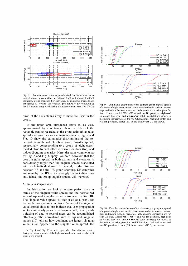
In order to estimate the angular spread of a group ofusers we will assume that each user fills a rectangulararea in the azimuth-elevation parameter space with sidesand center given by the instantaneous angular spreadsand mean angles, respectively, computed according toSec. III. Fig. 8 illustrates this situation for the case ofnine users located close to each other in various outdoor(top) and indoor scenarios (bottom).

We define the angular spread of a group of usersas the union of the areas occupied by their respectiverectangles. Intuitively, users with non-overlapping rect-angles offer good angular separation and, hence, weexpect the BS to be able to resolve them. Users withoverlapping rectangles may be resolved if the groupangular spread is “large enough”; that is, if the groupangular spread covers, at least, as many “resolution

0 50 100 150 200 250 300 3500

50

100

150

Azimuth [deg]

Ele

vation [deg]

Outdoor (low−roof)

MS 1 (LOS)

MS 2 (LOS)

MS 3 (NLOS)

MS 4 (NLOS)

0 50 100 150 200 250 300 3500

50

100

150

Azimuth [deg]

Ele

vation [deg]

Indoor (UE center)

BS 1

BS 3

Fig. 8. Instantaneous power angle-of-arrival density of nine userslocated close to each other in outdoor (top) and indoor (bottom)scenarios, at one snapshot. For each user, instantaneous mean delaysare marked as crosses. The overlaid grid indicates the resolution ofthe BS antenna array used during the measurements (see Sec. IV-D.)

bins” of the BS antenna array as there are users in thegroup.

If the union area introduced above is, as well,approximated by a rectangle, then the sides of therectangle can be regarded as the group azimuth angularspread and group elevation angular spreads. Fig. 9 andFig. 10 show the cumulative distributions of the so-defined azimuth and elevation group angular spread,respectively, corresponding to a group of eight users1

located close to each other in various outdoor (top) andindoor (bottom) scenarios. Here, the same comments asfor Fig. 5 and Fig. 6 apply. We note, however, that thegroup angular spread in both azimuth and elevation isconsiderably larger than the angular spread associatedwith each individual user. In general, as the distancebetween BS and the UE group shortens, UE centroidsare seen by the BS at increasingly distinct directionsand, hence, the group angular spread will increase.

C. System Performance

In this section we look at system performance interms of the singular value spread and the normalizedsum of squared singular values introduced in Sec. III.The singular value spread is often used as a proxy forfavorable propagation conditions. Values of the singularvalue spread close to one indicate that user propagationvectors are nearly pairwise orthogonal and, hence, mul-tiplexing of data to several users can be accomplishedeffectively. The normalized sum of squared singularvalues (10) tells us how dominant the largest singularvalue is. As opposed to the singular value spread, the

1In Fig. 9 and Fig. 10 we use eight rather than nine users sinceduring the measurements of the high-roof outdoor scenarios only eightusers were present.

50 100 150 200 250 300 3500

0.5

1

Sφ

(g) [deg]

Pro

b(S

φ(g) ≤

abscis

sa)

Outdoor

MS 1 (LOS)

MS 2 (LOS)

MS 3 (NLOS)

MS 4 (NLOS)

50 100 150 200 250 300 3500

0.5

1

Sφ

(g) [deg]

Pro

b(S

φ(g) ≤

abscis

sa)

Indoor

BS 1 (UE back)

BS 3 (UE back)

BS 1 (UE center)

BS 3 (UE center)

Fig. 9. Cumulative distribution of the azimuth group angular spreadof a group of eight users located close to each other in various outdoor(top) and indoor (bottom) scenarios. In the outdoor scenarios, plots forfour UE sites, labeled MS 1–MS 4, and two BS positions, high-roof(in dashed line style) and low-roof (in solid line style) are shown. Inthe indoor scenarios, plots for two UE locations, back and center, andtwo BS positions, center (BS 1) and corner (BS 3), are shown.

0 10 20 30 40 50 60 70 800

0.5

1

Sθ

(g) [deg]

Pro

b(S

θ(g) ≤

abscis

sa)

Outdoor

MS 1 (LOS)

MS 2 (LOS)

MS 3 (NLOS)

MS 4 (NLOS)

0 10 20 30 40 50 60 70 800

0.5

1

Sθ

(g) [deg]

Pro

b(S

θ(g) ≤

abscis

sa)

Indoor

BS 1 (UE back)

BS 3 (UE back)

BS 1 (UE center)

BS 3 (UE center)

Fig. 10. Cumulative distribution of the elevation group angular spreadof a group of eight users located close to each other in various outdoor(top) and indoor (bottom) scenarios. In the outdoor scenarios, plots forfour UE sites, labeled MS 1–MS 4, and two BS positions, high-roof(in dashed line style) and low-roof (in solid line style) are shown. Inthe indoor scenarios, plots for two UE locations, back and center, andtwo BS positions, center (BS 1) and corner (BS 3), are shown.

2 4 6 80

2

4

6

8

10

12Outdoor

Number of Users in Group

Sin

gula

r V

alu

e S

pre

ad [dB

]

MS 1 (high−roof)

MS 2 (high−roof)

MS 1 (low−roof)

MS 2 (low−roof)

2 4 6 80

2

4

6

8

10

12Indoor

Number of Users in Group

Sin

gula

r V

alu

e S

pre

ad [dB

]

BS 1 (UE back)

BS 3 (UE back)

BS 1 (UE center)

BS 3 (UE center)

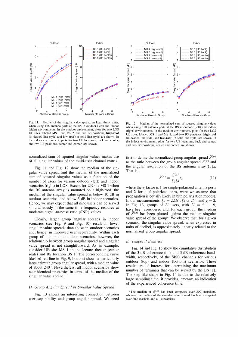
Fig. 11. Median of the singular value spread, in logarithmic units,when using 128 antenna ports at the BS in outdoor (left) and indoor(right) environments. In the outdoor environment, plots for two LOSUE sites, labeled MS 1 and MS 2, and two BS positions, high-roof(in dashed line style) and low-roof (in solid line style) are shown. Inthe indoor environment, plots for two UE locations, back and center,and two BS positions, center and corner, are shown.

normalized sum of squared singular values makes useof all singular values of the multi-user channel matrix.

Fig. 11 and Fig. 12 show the median of the sin-gular value spread and the median of the normalizedsum of squared singular values as a function of thenumber of users for various outdoor (left) and indoorscenarios (right) in LOS. Except for UE site MS 1 whenthe BS antenna array is mounted on a high-roof, themedian of the singular value spread is below 10 dB inoutdoor scenarios, and below 5 dB in indoor scenarios.Hence, we may expect that all nine users can be servedsimultaneously in the same time-frequency resource atmoderate signal-to-noise ratio (SNR) values.

Clearly, larger group angular spreads in indoorscenarios (see Fig. 9 and Fig. 10) result in lowersingular value spreads than those in outdoor scenariosand, hence, in improved user separability. Within eachgroup of indoor and outdoor scenarios, however, therelationship between group angular spread and singularvalue spread is not straightforward. As an example,consider UE site MS 1 in the lecture theater (centerseats) and BS location BS 1. The corresponding curve(dashed red line in Fig. 9, bottom) shows a particularlylarge azimuth group angular spread, with a median valueof about 240◦. Nevertheless, all indoor scenarios shownear identical properties in terms of the median of thesingular value spread.

D. Group Angular Spread vs Singular Value Spread

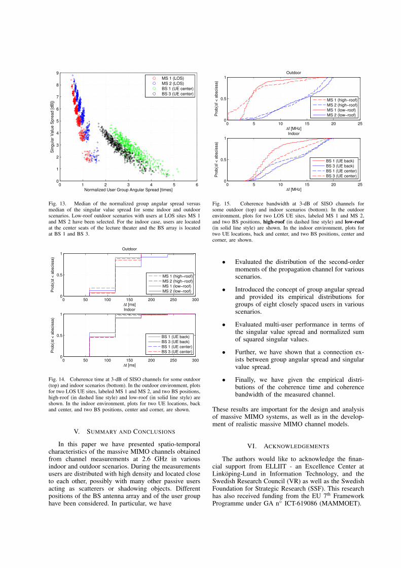
Fig. 13 shows an interesting connection betweenuser separability and group angular spread. We need

2 4 6 80

1

2

3

4

5

6

7

8

9Outdoor

Number of Users in Group

Sin

gu

lar

Va

lue

Sp

rea

d [

dB

]

MS 1 (high−roof)

MS 2 (high−roof)

MS 1 (low−roof)

MS 2 (low−roof)

2 4 6 80

1

2

3

4

5

6

7

8

9Indoor

Number of Users in Group

Sin

gu

lar

Va

lue

Sp

rea

d [

dB

]

BS 1 (UE back)

BS 3 (UE back)

BS 1 (UE center)

BS 3 (UE center)

Fig. 12. Median of the normalized sum of squared singular valueswhen using 128 antenna ports at the BS in outdoor (left) and indoor(right) environments. In the outdoor environment, plots for two LOSUE sites, labeled MS 1 and MS 2, and two BS positions, high-roof(in dashed line style) and low-roof (in solid line style) are shown. Inthe indoor environment, plots for two UE locations, back and center,and two BS positions, center and corner, are shown.

first to define the normalized group angular spread S(g)

as the ratio between the group angular spread S(g) andthe angular resolution of the BS antenna array ξφξθ.That is,

S(g) =S(g)

ξφξθχ, (11)

where the χ factor is 1 for single-polarized antenna portsand 2 for dual-polarized ones, were we assume thatpropagation is equally likely in bith polarization modes).In our measurements, ξφ = 22.5◦, ξθ ' 25◦, and χ = 2.In Fig. 13, groups of K users, with K = 2, . . . , 9,have been considered and, for each group, the medianof S(g) has been plotted against the median singularvalue spread of the group2. We observe that, for a givenscenario, the singular value spread, when expressed inunits of decibel, is approximately linearly related to thenormalized group angular spread.

E. Temporal Behavior

Fig. 14 and Fig. 15 show the cumulative distributionof the 3-dB coherence time and 3-dB coherence band-width, respectively, of the SISO channels for variousoutdoor (top) and indoor (bottom) scenarios. Theseresults are of interest for determining the maximumnumber of terminals that can be served by the BS [1].The step-like shape in Fig. 14 is due to the relativelylarge sampling time; it provides, anyway, an indicationof the experienced coherence time.

2The median of S(g) has been computed over 300 snapshots,whereas the median of the singular value spread has been computedover 300 snashots and all subcarriers.

0 1 2 3 4 5 60

1

2

3

4

5

6

7

8

9

Normalized User Group Angular Spread [times]

Sin

gu

lar

Va

lue

Sp

rea

d [

dB

])

MS 1 (LOS)

MS 2 (LOS)

BS 1 (UE center)

BS 3 (UE center)

Fig. 13. Median of the normalized group angular spread versusmedian of the singular value spread for some indoor and outdoorscenarios. Low-roof outdoor scenarios with users at LOS sites MS 1and MS 2 have been selected. For the indoor case, users are locatedat the center seats of the lecture theater and the BS array is locatedat BS 1 and BS 3.

0 50 100 150 200 250 3000

0.5

1

∆t [ms]

Pro

b(∆

t <

abscis

sa)

Outdoor

MS 1 (high−roof)

MS 2 (high−roof)

MS 1 (low−roof)

MS 2 (low−roof)

0 50 100 150 200 250 3000

0.5

1

∆t [ms]

Pro

b(∆

t <

abscis

sa)

Indoor

BS 1 (UE back)

BS 3 (UE back)

BS 1 (UE center)

BS 3 (UE center)

Fig. 14. Coherence time at 3-dB of SISO channels for some outdoor(top) and indoor scenarios (bottom). In the outdoor environment, plotsfor two LOS UE sites, labeled MS 1 and MS 2, and two BS positions,high-roof (in dashed line style) and low-roof (in solid line style) areshown. In the indoor environment, plots for two UE locations, backand center, and two BS positions, center and corner, are shown.

V. SUMMARY AND CONCLUSIONS

In this paper we have presented spatio-temporalcharacteristics of the massive MIMO channels obtainedfrom channel measurements at 2.6 GHz in variousindoor and outdoor scenarios. During the measurementsusers are distributed with high density and located closeto each other, possibly with many other passive usersacting as scatterers or shadowing objects. Differentpositions of the BS antenna array and of the user grouphave been considered. In particular, we have

0 5 10 15 20 250

0.5

1

∆f [MHz]

Pro

b(∆

f <

abscis

sa)

Outdoor

MS 1 (high−roof)

MS 2 (high−roof)

MS 1 (low−roof)

MS 2 (low−roof)

0 5 10 15 20 250

0.5

1

∆f [MHz]

Pro

b(∆

f <

abscis

sa)

Indoor

BS 1 (UE back)

BS 3 (UE back)

BS 1 (UE center)

BS 3 (UE center)

Fig. 15. Coherence bandwidth at 3-dB of SISO channels forsome outdoor (top) and indoor scenarios (bottom). In the outdoorenvironment, plots for two LOS UE sites, labeled MS 1 and MS 2,and two BS positions, high-roof (in dashed line style) and low-roof(in solid line style) are shown. In the indoor environment, plots fortwo UE locations, back and center, and two BS positions, center andcorner, are shown.

• Evaluated the distribution of the second-ordermoments of the propagation channel for variousscenarios.

• Introduced the concept of group angular spreadand provided its empirical distributions forgroups of eight closely spaced users in variousscenarios.

• Evaluated multi-user performance in terms ofthe singular value spread and normalized sumof squared singular values.

• Further, we have shown that a connection ex-ists between group angular spread and singularvalue spread.

• Finally, we have given the empirical distri-butions of the coherence time and coherencebandwidth of the measured channel.

These results are important for the design and analysisof massive MIMO systems, as well as in the develop-ment of realistic massive MIMO channel models.

VI. ACKNOWLEDGEMENTS

The authors would like to acknowledge the finan-cial support from ELLIIT - an Excellence Center atLinkoping-Lund in Information Technology, and theSwedish Research Council (VR) as well as the SwedishFoundation for Strategic Research (SSF). This researchhas also received funding from the EU 7th FrameworkProgramme under GA n◦ ICT-619086 (MAMMOET).

REFERENCES

[1] T. L. Marzetta, “Noncooperative cellular wireless with unlim-ited number of base station antennas,” IEEE Trans. WirelessCommun., vol. 9, pp. 3590–3600, Nov. 2010.

[2] F. Rusek, D. Persson, B. K. Lau, E. G. Larsson, T. L. Marzetta,O. Edfors, and F. Tufvesson, “Scaling up MIMO: Opportunitiesand challenges with very large arrays,” IEEE Signal Process.Mag., vol. 30, pp. 40–60, Jan. 2013.

[3] E. G. Larsson, F. Tufvesson, O. Edfors, and T. L. Marzetta,“Massive MIMO for next generation wireless systems,” IEEECommun. Mag., vol. 52, pp. 186–195, Feb. 2014.

[4] H. Q. Ngo, E. G. Larsson, and T. L. Marzetta, “Energy andspectral efficiency of very large multiuser MIMO systems,”IEEE Trans. Wireless Commun., vol. 61, pp. 1436–1449, Apr.2013.

[5] J. Andrews, S. Buzzi, C. Wan, S. Hanly, A. Lozano, A. Soong,and J. Zhang, “What will 5G be?,” IEEE J. Sel. Areas Commun.,vol. 32, pp. 1065–1082, June 2014.

[6] F. Boccardi, R. Heath, A. Lozano, T. Marzetta, and P. Popovski,“Five disruptive techonology directions for 5G,” IEEE Com-mun. Mag., vol. 52, pp. 74–80, Feb. 2014.

[7] A. Osseiran, F. Boccardi, V. Braun, K. Kusume, P. Marsch,M. Maternia, O. Queseth, M. Schellmann, H. Schotten,H. Taoka, H. Tullberg, M. Uusitalo, B. Timus, and M. Fallgren,“Scenarios for 5G mobile and wireless communications: thevision of the METIS project,” IEEE Commun. Mag., vol. 52,pp. 26–35, May 2014.

[8] S. Payami and F. Tufvesson, “Channel measurements andanalysis for very-large array systems at 2.6 GHz,” in Proc.EuCAP 2012 - 6th European Conf. in Ant. and Prop., pp. 433–437, Mar. 2012.

[9] X. Gao, F. Tufvesson, O. Edfors, and F. Rusek, “Measuredpropagation characteristics for very-large MIMO at 2.6 GHz,”in Proc. ASILOMAR 2013 - 46th Conf. on Sig., Syst. andComput., pp. 295–299, Nov. 2012.

[10] X. Gao, O. Edfors, F. Rusek, and F. Tufvesson, “MassiveMIMO in real propagation environments,” arXiv:1403.3376[cs.IT], Submitted to IEEE Trans. Wireless Commun.

[11] X. Gao, O. Edfors, F. Rusek, and F. Tufvesson, “Linear pre-coding performance in measured very-large MIMO channels,”in Proc. VTC 2011 Fall - IEEE 74th Vehicular TechnologyConf., pp. 1–5, Sept. 2011.

[12] J. Hoydis, C. Hoek, T. Wild, and S. ten Brink, “Channelmeasurements for large antenna arrays,” in Proc. ISWCS 2012- IEEE 9th Int. Symp. on Wireless Commun. Syst., vol. IT-29,pp. 811–815, Aug. 2012.

[13] J. Flordelis, X. Gao, G. Dahman, F. Rusek, O. Edfors, andF. Tufvesson, “Spatial separation of closely-spaced users inmeasured massive multi-user MIMO channels,” in Proc. ICC2015 - IEEE Int. Conf. Commun., June forthcoming.

[14] E. Karipidis, J. Lorca, and E. Bjornsson, “System scenarios andrequirements specifications,” tech. rep., MAMMOET, 2015.

[15] A. Bourdoux, C. Desset, L. van der Perre, G. Dahman,O. Edfors, J. Flordelis, X. Gao, C. Gustafson, F. Tufvesson,F. Harrysson, and J. Medbo, “MaMi channel characteristics:Measurement results,” tech. rep., FP7 MAMMOET, July 2015.

[16] R. S. Thoma, D. Hampicke, A. Richter, G. Sommerkorn,A. Schneider, U. Trautwein, and W. Wirnitzer, “Identificationof time-variant directional mobile radio channels,” IEEE Trans.Instrum. Meas., vol. 49, pp. 357–364, Apr. 2000.

[17] M. Steinbauer, A. F. Molisch, and E. Bonek, “The double-directional radio channel,” IEEE Trans. Antennas Propag.,vol. 43, pp. 51–63, Aug. 2001.

[18] A. F. Molisch, Wireless Communications. New York: JohnWiley & Sons, 2011.

[19] B. Fleury, M. Tschudin, R. Heddergott, D. Dalhaus, andK. Ingeman-Pedersen, “Channel parameter estimation in mobileradio environments using the sage algorithm,” IEEE J. Sel.Areas Commun., vol. 17, no. 3, pp. 434–450, 1999.

[20] B. Fleury, “First- and second-order characterization of directiondispersion and space selectivity in the radio channel,” IEEETrans. Inf. Theory, vol. 46, no. 6, pp. 2027–2044, 2000.

[21] A. Adhikary, N. Junyoung, A. Jae-Young, and G. Caire,“Joint spatial division and multiplexing — the large-scale arrayregime,” IEEE Trans. Inf. Theory, vol. 59, pp. 6441–6463, June2013.

[22] N. Junyoung, A. Adhikary, A. Jae-Young, and G. Caire, “Jointspatial division and multiplexing: Opportunistic beamforming,user grouping and simplified downlink scheduling,” IEEE J.Sel. Topics Signal Process., vol. 8, pp. 876–890, Mar. 2014.