Inhouse Software Develop-

ment For 3D microscopy and modelling and other scientific issues, the laboratory of concrete and construction chemistry develops and supports a software toolbox for quantitative imaging which is freely distributed (conditions see below).

Inhaltsverzeichnis 1 Quantitative imaging ..................................................................................................................................... 3

2 Image processing platform .......................................................................................................................... 3

3 Inhouse software development for ImageJ ........................................................................................... 3

4 Conditions for free usage and download............................................................................................... 4

5 Data import ........................................................................................................................................................ 4

6 Filtering ............................................................................................................................................................... 5

1. Anisotropic Diffusion ............................................................................................................................ 5 6.1 Canny Edge ............................................................................................................................................... 7 6.2 Cluster Image ........................................................................................................................................... 9 6.3 Disconnect Particles ............................................................................................................................ 11

6.3.1 Distance Transform .................................................................................................................... 12

6.4 FFT 2D 3D ................................................................................................................................................ 13 6.5 Image Calculator ................................................................................................................................... 15 6.6 Labelling 2D 3D ..................................................................................................................................... 17 6.7 Remove Background ........................................................................................................................... 18 6.8 Roundness 2D 3D ................................................................................................................................. 20 6.9 Skeletonization 2D 3D ........................................................................................................................ 21

7 Stripe Filter ....................................................................................................................................................... 22

8 Reconstruction ................................................................................................................................................ 24

8.1 Filtered Backprojection ...................................................................................................................... 25 8.2 Projections Sinograms ........................................................................................................................ 25 8.3 Reconstruct 3D from 2D .................................................................................................................... 25

9 Evaluation ......................................................................................................................................................... 27

9.1 Particle Size Distribution .................................................................................................................... 27 9.2 Phase Image Evaluation ..................................................................................................................... 29 9.3 Pore Size Distribution ......................................................................................................................... 31

10 Editors and Viewers .................................................................................................................................. 32

10.1 Display Volume ..................................................................................................................................... 33 10.2 Edit Label Region .................................................................................................................................. 34 10.3 Segment Phases 3D ............................................................................................................................. 35 10.4 View 3D Mask ........................................................................................................................................ 36

1 Quantitative imaging 3D microscopy and modelling is usually based on quantitative imaging. In contrast to quali-tative imaging serving as the basis for image enhancement for perceptual inspection, quanti-tative imaging yields the background for parametric studies by providing user-independent and thus reproducible sets of values. Quantitative imaging can either be applied to 2D imag-es as well as to subsequent stacks of images representing volumetric 3D data of a sample. In the analysis of cement pastes and mortars as in many other scientific fields, the veritable 3D context of the investigated specimen is often inevitable in order to correctly comprehend volumetric structural features.

2 Image processing platform ImageJ has been selected because it is a public domain, user friendly and extensible platform for 2D as well as for 3D image processing and analysis. It is designed by using an open archi-tecture and provides extensibility via Java plugins. The source is freely available from http://imagej.nih.gov/ij/. It is designed and maintained by Wayne S. Rasband from the U.S. National Institutes of Health, Bethesda, Maryland, USA.

Its programming language is Java. Java is a free high level language using the concept of a virtual processor. Hence, it enables high portability on all operating systems supporting the java runtime engine, at least on all UNIX, MacIntosh and Microsoft operating systems.

Since ImageJ is being widely used, a respectable bunch of plugins is already available on the net. The smartly designed open architecture of ImageJ is inviting for further extensions.

3 Inhouse software development for ImageJ

A set of prospective ImageJ plugins is maintained by the group for 3D-Microscopy, Analysis and Modelling of the Laboratory for Concrete and Construction Chemistry at Empa. The plugins include automated imaging tools for filtering, data reconstruction, quantitative data evaluation and data import, as well tools for interactive segmentation, visualization and man-agement of image data.

Since the research focus of our group is on 3D imaging, all of our plugins are able to deal with either 2D or 3D image data. 3D image data in ImageJ is represented by image stacks. 3D processing may include slice-wise 2D processing of all images in the stack or, more im-portant, true 3D processing.

Each one of the new plugins includes a help button where general remarks about the func-tionality and a description of the parameters is provided. This feature does not correspond with the ImageJ philosophy assuming the help documentation to be available on the internet. However, we consider the help button as a handy feature.

The user might be surprised to realize that some of the tools are apparently already existing in other plugins of ImageJ or Fiji. Those tools are for instance “FFT”, “Image Calculator”, “Dis-tance Transform” and others. The reason for this apparent re-duplication is that the original tools incorporate major restrictions which are elimintated in the newplugins. Each one of the available tools and its advantage is shortly being presented below.

4 Conditions for free usage and download

The ImageJ plugins are included into the library file "xlib_.jar" and can be freely downloaded from the ftp server at

ftp://ftp.empa.ch/pub/empa/outgoing/BeatsRamsch/lib/

Use an Explorer (not the Internet Explorer), enter the address and log in by giving "anony-mous" as the user name and type your email address for the password. For adding the li-brary to ImageJ, please follow the instructions in the "ReadMe.txt" file. The new plugins can then be found under PluginsBeat.

The plugins are provided „as is“ with no further support guaranteed; any liability for loss of data or any other damage arising from its use is disclaimed. The use of the offered plugins is free, provided that they are neither integrated into commercial products nor used for any other kind of profit. If the software is being used for research, Empa as owner of the Software is mandatory to be mentioned in the acknowledgements, and for citing the respective papers indicated in the help text.

5 Data import Plugins of this section offer the capability to import special data formats that are unknown to ImageJ, but interesting for usage.

Import DMP

DMP is a simple format for storing 2D images. It is used at IBT from the ETH and University of Zurich. The first two short entries of the data file are reserved for providing the width and

the heigth of the image. The next short entry is reserved. After that (i.e. after the first 6 bytes) follows the image data itself, each pixel given by a 32-bit floating number.

A short Matlab code for writing such an image "image" with the size "width" and "heigth" is given below:

fid = fopen(file, 'w'); fwrite(fid, width, 'uint16'); fwrite(fid, height, 'uint16'); fwrite(fid, 0, 'uint16'); fwrite(fid, image', 'float32'); fclose(fid);

Reading the DMP image with Matlab can be achieved like this:

fid = fopen(filename); dim = fread(fid, 3, 'uint16'); width = dim(1); height = dim(2); data = zeros(width, height); for ii=1:height data(:,ii) = fread(fid, width, 'float32'); end fclose(fid);

6 Filtering The filtering functions accept one or more images or stacks of images where some filtering technique are applied to. Generally, the filtering functions work on 2D images, slice-wise 2D, as well as in true 3D mode if it is applied to image stacks.

1. Anisotropic Diffusion The mechanism of heat diffusion has been used as the basics for image filtering. Thereby, the image values are understood as temperature values and image blurring represents the process of heat transport blurring. The key idea is the introduction of anisotropy, i.e. of diffu-sion characteristics that are depending on the pixel environment and the transfer direction. The local anisotropy is assigned according to the direction and magnitude of the image gra-dient, introducing high diffusion rates at low gradients and low diffusion rates at high gradi-ents. Hence, the anisotropic diffusion characteristics are defined according to an ellipse in 2D or an ellipsoid in 3D perpendicular to the gradient vector.

The corresponding partial differential equation had first been numerically approached in 1990 by a fast algorithm of Perona and Malik [1] by defining the elliptic diffusion shapes by

means of simple box filtering. Way better results can be obtained with the technique of Tschumperlé and Deriche [2] from 2005 by setting the tensor field according to the Eigenval-ues and Eigenvectors in order to drive the diffusion. As expected, this approach is however more time consuming.

The filter is a brilliant edge preserving / smoothing filter for intelligent noise reduction. In particular the implementation of Tschumperlé and Deriche outperforms other approaches in respect of the distinction between coherent edges and noise. Fig.6.1 shows a comparison between anisotropic diffusion (bottom right) and median filtering (bottom left) of a CT slice from concrete after strong alcali aggregate reactions (top). Anisotropic diffusion filtering is outstanding by better preserving the cracks while flattening inhomogeneities due to noise (please note center regions).

The filter works in 2D as well as in 3D.

Fig.6.1: CT slice after strong alcali aggregate reactions (top) and edge preserving / smoothing filtering with a 4x4 median (bottom left) and anisotropic diffusion (bottom right).

References:

1 - Perona P, Malik J., "Scale-Space and Edge-Detection Using Anisotropic Diffusion", IEEE Trans. Pattern Anal. Mach. Intell. 12(7), pp.629-639, 1990.

2 - Tschmperlé D, Deriche R., "Vector-Valued Image Regularization with PDE's: A Common Framework for Different Applications", IEEE Trans. Pat. Anal. Mach, Intell,. 27(4): 506-517, 2005.

6.1 Canny Edge In 1986, J. Canny has proposed an excellent edge detection filter [3] that due to its perfor-mance became famous. The filter is based on a fast numeric approach for the calculation of the direction-dependent first derivative, i.e. the gradient vector function of an image. The Canny filter is well known for 2D imaging, yet it is barely supported in 3D. This plugin sup-ports both, the 2D and the 3D implementation. It additionally supports preceding Gauss fil-tering, optional non-maxima suppression for the extraction of the edges, as well as a function for double thresholding and joining the connected regions. Double thresholding means that an upper threshold is used for extracting the relevant edges, while a lower threshold is pro-vided for adding residing connections between the extracted edges. The plugin returns the magnitudes and the angles of the gradient vector functions.

The results of a Canny filtered image of a valve image is shown in Fig.6.2 (top: original im-age). The gradient magnitude and angles are presented (2nd row), as well as the magnitudes after non-maxima suppression and also after joining the connected regions (3rd row).

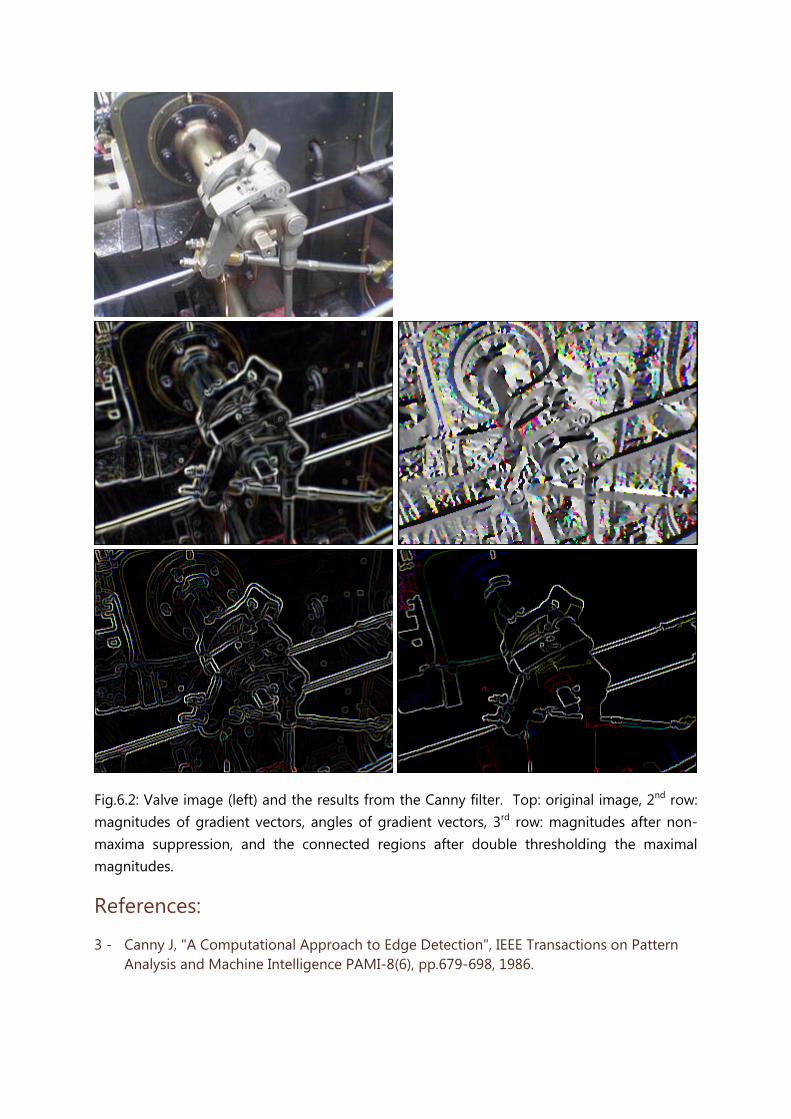
Fig.6.2: Valve image (left) and the results from the Canny filter. Top: original image, 2nd row: magnitudes of gradient vectors, angles of gradient vectors, 3rd row: magnitudes after non-maxima suppression, and the connected regions after double thresholding the maximal magnitudes.

References:

3 - Canny J, "A Computational Approach to Edge Detection", IEEE Transactions on Pattern Analysis and Machine Intelligence PAMI-8(6), pp.679-698, 1986.

6.2 Cluster Image Cluster analysis is a technique of statistical data analysis for grouping sets of objects. It is used in machine learning, data mining, pattern recognition, information retrieval, bio-informatics and can also be applied to image analysis. Different clustering definitions and al-gorithms have been proposed using connectivity, distance to the cluster center, statistical distribution, or density rates as optimization parameters for building clusters.

In image analysis, mainly two algorithms are prominent: the k-means algorithm and the mean shift algorithm. They have been implemented together with a third one, fuzzy c-means clustering.

The k-means algorithm [4] minimizes the square sum of the distances of each data point to its assigned cluster center. It starts with a random association of the data points to an initial-ly determined number of clusters. Using an iterative optimization procedure it converges quickly to stable data assignments to clusters. K-means clustering is popular because it is very fast.

The mean shift clustering method [5] optimizes the cluster centers such that the data densi-ties within the clusters which are maximized. Within kernels of a given size around each data point, the centeroid of all points inside of the kernel is determined and the sphere shifted ac-cordingly. After iterative repetition of this process, the sphere remains stationary. The data point is then assigned to this final cluster center. The algorithm can be understood as like the walk to the closest peak in a mountain landscape. Within a certain perimeter, the highest target is being located and reached. From thereon, the next target within the same perimeter is located and reached again. This process is iteratively carried on until the top within the se-lected perimeter is reached. Depending on the perimeter size, different hills or sub-hills will be achieved. If the perimeter is larger than 400km, you will reach the Mont Blanc from any-where in Switzerland. If it is larger than 20'000km, the Mount Everest will be reached from any point in the world. If its size is only a some meters, you will probably end up on the top of a building.

Fuzzy c-means clustering [6] allows a data point to be assigned to more than one clusters. The affiliation to a cluster is given by a membership value ranging from zero to one. The sum of all memberships for a data point is unity. Hence, the assignment of a data point to a class is not unequivocal but relative. The degree of belonging to a class is related inversely to the distance from the data point to the cluster. It also depends on a parameter that controls how much weight is given to the winning cluster. With fuzzy c-means, the centroid of a cluster is the mean of all points, weighted by their degree of belonging to the cluster. The finally win-ning class is the one with the highest ranking. The process of the fuzzy c-means algorithm is very similar to the k-means algorithm.

As an example, ESEM images of a natural cement analogue (Maqarin, Jordania) is provided in Fig.6.3.1. A back-scatter electron microscope (BSE) image (top left) and image maps acquired from energy-dispersive X-ray spectroscopy (EDX) at the same location forked into 14 differ-

ent elements (see Fig.6.3.1) are used as the basis for clustering. Thus together with the BSE image, the clustering is achieved from a 15-dimensional vector space. In Fig.6.3.2 some re-sults from different clustering algorithms and parameter settings are displayed. The first row shows results from the k-means, the second one from the mean shift, and the third one from fuzzy c-means clustering. K-means clustering (1st row) requires the number of clusters as an input parameter. The results for 2 (left), 3, 5 and 16 (right) clusters are provided. Slightly dif-ferent results provides mean shift clustering (2nd row) which requires the size of the seeking perimeter as input parameter. It is determined at 100 (left), 70, 60 and at 50 (right). Fuzzy c-means clustering (3rd row) requires the number of clusters and the fuzziness as input param-eters. The results are displayed for 5 clusters at fuzziness 1.1 (left) and 4.0, for 16 clusters at fuzziness 2.0, as well as an image showing its fuzziness membership to the cluster with the highest respective ranking at each location (right).

Clustering can also be applied to one dimensional spaces (i.e. from a single gray level image), or for color images where the R, G, B color channels provide a 3-dimensional vector space. Clustering thus provides an elegant way for automatic segmentation of 2D images or 3D im-age volumes containing different phases.

Fig.6.3.1: Image acquired by BSE and EDX maps at the same local position showing the amounts of Ca, C (1st row), Al, Cl, Fe, K (2nd row), Mg, Mn, Na, O (3rd row), P, Si, S, Ti (4th row).

Fig.6.3.2: Results from clustering of the 15-dimensional image data space displayed in Fig.6.3.1. First row: k-means for 2 (left), 3, 5 and 16 (right) clusters. Second row: mean shift for the seeking perimeters 100 (left), 70, 60 and 50 (right). Third row: fuzzy c-means cluster-ing for 5 clusters at fuzziness 1.1 (left) and 4.0, 16 clusters at fuzziness 2.0, and its fuzziness membership values (right).

References:

4 - Kanungo T., Mount D.M., Netanyahu N.S., Piatko C.D., Silverman R., Wu A.Y., "An efficient k-means clustering algorithm: Analysis and implementation", IEEE Trans. Pattern Analysis and Machine Intelligence 24(7), pp.881-892, 2002.

5 - Funkunaga K., Hosteler L.D., "The Estimation of the Gradient of a Density Function, with Applications in Pattern Recognition", IEEETransactions on Information Theory 21(1), pp.32-40, 1975.

6 - Bezdek J.C., "FCM: The fuzzy c-means clustering algorithm", Computers & Geosciences 10(2), pp.191-203, 1984.

6.3 Disconnect Particles In particle analysis from imaging due to the resolution limits, the particles might be wrongly connected at various locations if they are located too close to each other. To remedy such connections, an algorithm for disconnecting them at their bottle necks has been implement-ed [7]. If requires a parameter k ranking from [0...1] controlling the disconnection. At k=1, particle separation occurs at any bottle necks while at k=0, no separation at all is being per-

formed. The optimum depends on the data and is usually somewhere around k=0.7 inducing marked bottle necks to be carved and small bottle necks to be left unchanged.

Results from cement grains acquired by 3D FIB-nanotomography are displayed in Fig.6.4. To the left, the original data volume is visualized. The center image shows the mask after image thresholding. Particles close to each other are erroneously interconnected at various loca-tions. The image to the right shows the volume disconnected at k=0.7 and labelled subse-quently.

Fig.6.4: 3D FIB-nanotomography of cement grains (left), subsequent thresholding (center), disconnected (k=0.7) and labelled particles (right).

References:

7 - Münch B., Gasser P., Holzer L., Flatt R., "FIB Nanotomography of Particulate Systems - Part II: Particle Recognition and Effect of Boundary Truncation.", Journal American Ce-ramics Society 89(8), pp.2586-2595, 2006.

6.3.1 Distance Transform Fast distance transform of image masks is useful for many morphological imaging applica-tions. In an age of increasing data size, processing speed is of ultimate priority. A modern approach [8], [9] allows the generation of the distance transform even in linear time. The im-plementation in this plugin allows the calculation of Euclidian, Chessboard, or Citymap dis-tance transform in both, 2D and 3D.

In Fig.6.5.1, a binary mask from cement particles (left) is processed by using the Euclidian dis-tance transform (center). The transform of the inverse mask is also given (right). The dis-tances are visualized by using a color lookup table from blue (low values) to red (high values). The effect of different distance metrics is displayed in Fig.6.5.2. A simple mask consisting of 3 single black dots is provided (left). Next to it, the results of the Euclidian, Chessboard and Citymap (right) distance transform is shown.

Fig.6.5.1: binary mask from cement particles (left) and Euclidian distance transform of it (cen-ter) and of its reversed mask (right).

Fig.6.5.2: Mask containing 3 black dots only (left) and its Euclidian, Chessboard and Citymap (right) distance transform.

References:

8 - Saito T, Toriwaki J.-I., "New algorithms for euclidean distance transformation of an n-dimensional digitized picture with applications", Pattern Recognition 27(11), pp.1551-1565, 1994.

9 - Meijster A., Roerdink J.B.T.M., Hesselink W.H., "A General Algorithm for Computing Dis-tance Transform in Linear Time", in Proc. Mathematical Morphology and its Applications to Image and Signal Processing, Kluwer, pp.331-340, 2000.

6.4 FFT 2D 3D The fast, well known and widely used Cooley-Tukey radix-2 algorithm for the calculation of the discrete fast Fourier transform (FFT) only works on data whose size is equal to a power of two. In order to provide FFT on data of different size, the data is usually extended to the next higher power of two. In many cases, this approach is sufficient, in particular if the periodical nature of the transformed data function is not relevant. However, if the period length is im-portant and must be left unchanged, FFT on the original data size is required. This can be achieved by using the Bluestein algorithm [10], [11]. Since to our best knowledge, there is no ImageJ plugin available that permits FFT for non-radix-2 sized periods, this plugin has been

built. It correctly calculates the complex FFT on 2D and 3D images of arbitrary size. It op-tionally provides the real and the imaginary part, or the magnitude and the angle images. Moreover, it allows a logarithmic or square-root based scaling to be introduced in order to lower the contrast among the FFT coefficients. This feature is useful if the FFT function is used for display purpose. The reversibility of the FFT transform is supported for all these op-tions.

In Fig.6.6 is a sample FIB-nt image from cement paste (left) with a width of 427 and a height of 768 pixels. The magnitudes and angles of its Fourier transform is scaled by a logarithmic funcion for improving the visibility of the small coefficients. The inverse FFT transform of the center and right images yields the original function (left) again without any loss of precision.

Fig.6.6: FIB-nt image (427x768 pixels) from cement paste (left) and the magnitudes (center) and angles (right) of its Fourier transform.

References:

10 - Bluestein L.I., "A linear filtering approach to the computation of the discrete Fourier transform", Northeast Electronics Research and Engineering Meeting Record 10, pp.218-219, 1968.

11 - Rabiner L.R., Schafer R.W., Rader C.M., "The chirp z-transform Algorithmus", IEEE Trans. Audio Electroacoustics 17(2), pp.86-92, 1969.

6.5 Image Calculator Many image calculators allowing various arithmetic operations are already implemented in ImageJ, including the "Image Calculator", the "Calculator Plus" as well as the entire list of functions in "math", all of them under "Process". So why "yet another image calculator", you might ask. The reason is that our image calculator is easily able to perform the possible tasks of all of the above listed plugins and much more. The conceptual idea is to provide a list of all the images and image stacks that are currently opened in ImageJ and assign them to symbolic names (i0, i1, i2,...). In a text field, the user can then provide his own code he wants to be applied to the images.

For instance,

(i0 + i1 + i2) / 3

will return an image providing the mean value of the images i0, i1 and i2.

The line

i0 + x

will calculate a copy of the image i0 overlayed by a horizontal ramp.

The line

Math.sqrt(Math.pow(100 - x, 2) + Math.pow(200 - y, 2)) // i0

calculates an image of the same size as image i0, but only containing a halo with the center of (100, 200).

The line

(i0 >= 128)? 255 : 0

creates a binary image mask by thresholding the image i0 with the value 128.

The above examples show that any pixel- or voxel-wise operation can be provided in a single command line as soon as it follows the Java notation.

The plugin is however able to do much more. Instead of pixelwise operation mode, image-wide Java code fragments can be provided. For example, the code fragment

double mean = 0; for (int ii = 0; ii < m0[0] * m0[1]; ii++) mean += i0[ii]; mean /= m0[0] * m0[1]; IJ.showMessage("mean value: " + mean); return null;

just calculates the overall mean value of image i0 and displays it in a check box. For more in-formation about the syntax, please consult the help function of the plugin itself. As a final example, we show that it is also possible to create images with that tool:

int max = 255; int mx = 512; int my = 512; float[] out = new float[mx * my]; for (int jj = 0; jj < my; jj++) for (int ii = 0; ii < mx; ii++) { double px = -2. + (double)ii / 200.; double py = -1. + (double)jj / 255.; double zx = 0.0, zy = 0.0; double zx2 = 0.0, zy2 = 0.0; int value = 0; while (value < max && zx2 + zy2 < 4.0) { zy = 2.0 * zx * zy + py; zx = zx2 - zy2 + px; zx2 = zx * zx; zy2 = zy * zy; value++; } out[ii + jj * mx] = 50f * (float)Math.log(value); } return new Object[] { new int[] { mx, my }, out };

This code fragment creates the image displayed in Fig.6.7 showing a well-known Mandelbrot fractal!

Fig.6.7: Mandelbrot fractal provided by the code above entered into the "Image Calculator" plugin.

6.6 Labelling 2D 3D Particle analysis requires labelling of the previously determined particle mask which has been obtained by some type of image segmentation technique, e.g. by thresholding to mention the most simple one. The binary particle mask allows evaluation of the particles only global-ly. By labelling the particles, each particle is assigned a unique ID. Labelling is the prerequi-site for evaluations considering local values such as particle size, diameter or other shape pa-rameters on the single objects. This plugin implements the labelling of disconnected objects in both, 2D or 3D binary masks. The binarization from gray level images occurs via providing a lower and an upper threshold.

An example of labelling is given in the center and right images of Fig.6.4, where the center image shows the particle mask before the disconnection procedure and before labelling. The disconnection procedure separates the single particles. After this step, the object mask is still binary and labelling is applied to colorize the particles in order to be able to distinguish them by their object values.

6.7 Remove Background If an image is subject to consistent global shifts of the image values depending on the loca-tion, this might be due to inconsistencies in the data acquisition rather than to real changes in the material properties. In that case, background removal techniques might be appropri-ate.

A typical example is image data from FIB-nanotomography (FIB-nt). Thereby, FIB-nt is ap-plied onto cubes that are engraved into the flat sample surface prior to data acquisition. Due to shadowing effects, the subsequent 3D data acquisition lacks in loss of brightness and con-trast towards the lower boundaries of the slices. This erroneously causes systematic inhomo-geneities of the image values impeding reliable quantitative imaging.

Correction of such deficits can be obtained by determining a global polynomial of low de-gree over the entire image and by subsequently subtracting the values of the polynomial function from the original image. The global polynomial function is determined by perform-ing least squares optimization. Accordingly, systematic brightness variations can be globally corrected. The necessary assumption is that the overall image values remain more or less constant over the entire image, at least in an average sense.

An example from a FIB-nt image and its shadowing effects is given in Fig.6.9.1 (top left). Af-ter thresholding, the systematic brightness loss towards the lower boundary becomes obvi-ous (top center). The determination of a global polynomial of degree 1 results in a back-ground image (top right). After subtraction (bottom left), the brightness drop disappears, as subsequent thresholding (bottom right) approves.

Fig.6.9.1: FIB-nt image with strong shadowing effects (top left), its thresholding (top centre), global polynomial of degree 1 (top right), its subtraction from the original image (bottom left), and its thresholding (bottom right).

In addition to the global homogeneization of the brightness values, the plugin also allows the correction of contrast values. However as an additional prerequisite, the image must be as-sumed to consist of a certain number of phases of more or less stable image values. In that case, a global polynomial can be calculated from the phase containing the lowermost image values, and a second polynomial from the phase containing the uppermost image values. The drifts are corrected by flattening both polynomial functions. The procedure hereby re-quires the number of phases as input parameter.

The results of this kind of correction is displayed in Fig.6.9.2. To the left, the original image is displayed. It consists of three different phases. Towards the lower border, a substantial drop of both, brightness and contrast occurs. Assuming a three phase image and after correction, the corrected image appears to be free from brightness and contrast drops (right).

Fig.6.9.2: FIB-nt image of a fuel cell and its shadowing effects (left), and the image after cor-rection (right) by assuming three existing phases.

6.8 Roundness 2D 3D The roundness value of a connected object can be defined as the ratio of the actual size of the object and the size of the virtual sphere spanned by the largest diameter of that object.

2D: rnd = 4. * size / (diameter^2 * PI) 3D: rnd = 6. * size / (diameter^3 * PI) Other well-known definitions (e.g. the definition of sphericity by Wadell [12]) are based on the surface area of the sphere with the same volume as the object, relative to its actual sur-face area. The calculation of the surface area on pixelized objects is not straight forward, whereas the calculation of the volume size is just the number of object pixels or voxels. That's the reason why we prefer the former roundness definition. Though, another useful op-tion for pixelized objects could be the roundness definition of ISO which is based on the ratio between inscribed and circumscribed circles of an object, i.e. the minimum and maximum siz-es for circles fitting inside and enclosing an object.

Roundness values are useful to provide a metric of how closely the shape of an object ap-proaches a circle (2D) or a sphere (3D), thus for rating object shapes.

References:

12 - Wadell H., "Volume, Shape and Roundness of Quartz Particles", Journal of Geology 43(3), pp.250-280, 1935.

6.9 Skeletonization 2D 3D In shape analysis, topological features can be captured from skeletons of the masks. Skele-tons have several different mathematical definitions in the technical literature. Many different algorithms have been proposed. Many of them lack in retaining the original topology. A good conservation of the topology in 2D as well as in 3D was the main reason for the choice of the algorithm (Palagyi, [13]). This feature is displayed in Fig.6.11, where a set of geomet-rical 3D objects is provided (left). After skeletonization (center), the topology is mainly being preserved. If the diameter of the skeletoized pipes is inflated up to the values from the dis-tance transform of original volume (right), the thus restored objects obtain high similarity to the original ones.

Fig.6.11: Some 3D objects (top), their skeletonization (bottom left) and their restoration by in-flating the pipes up to the distance transform values of the original objects (bottom right).

References:

13 - Palagyi K., Kuba A., "A 3D6-subiteration thinning algorithm for extracting medial lines", Pattern Recognition Letters 19, pp.613-227, 1998.

7 Stripe Filter Striping artifacts may occur due to undesired effects during data acquisition. Defect detector pixels might be the reason of stripes in the projections of computed tomography measure-ments resulting in ring artifacts after reconstruction. Waterfall artifacts might be the reason for stripes when accessing 3D data using FIB-nanotomography. Both types of artifacts can be erased by a technique for stripe filtering based on the combination of Wavelet and Fourier transform [14]. The potential of the stripe filtering plugin is shown in Fig.6.12.1 by applying it to a gray level image (top) and to a RGB image (bottom). In Fig.6.12.2, the stripes in CT pro-jections (top) and the resulting ring artifacts in the reconstructed images (bottom) is present-ed, the original situation to the left and the results after stripe filtering to the right.

Fig.6.12.1: Gray level (top) and RGB (bottom) image containing horizontal stripes (left) and the results of the stripe filtering plugin (right).

Fig.6.12.2: Projection image in a CT slice (top) before (left) and after (right) stripe filtering. The stripes in the projections yield ring artifacts in the reconstructed image (bottom). An original (left) and its filtered version (right) is displayed.

References:

14 - Münch B., Trtik P., Marone F., Stampanoni M., "Stripe and ring artifact removal with com-bined wavelet-Fourier filtering", Optical Express 17(10), pp.8567-8591, 2009.

8 Reconstruction Plugins of this section support preprocessing and reconstruction of images from projection data for CT imaging.

Another category of methods in this section is the estimation of 3D data from 2D images with the idea of estimating parameters requesting 3D connectivity from 2D slices only.

8.1 Filtered Backprojection This plugin provides convolution / backprojection of a set of projections to an image. It sup-ports different reconstruction filters (Shepp & Logan, Parzen, Hamming, Hann, Rectangular). The sequence of angles as well as the sequence of the projections can be altered.

8.2 Projections Sinograms This plugin converts sets of projections into stacks of sinograms and vice versa. It also sup-ports flat and dark field correction, speckle filtering, Lambert inversion, adjustment of the ro-tation center, re-ordering of the projections, adjustment of the value range, etc.

8.3 Reconstruct 3D from 2D This plugin provides the reconstruction of virtual 3D phase volumes from 2D phase images. The goal is to preserve the structural characteristics given in the 2D image and to extrapolate it to 3D.

The algorithm assumes that the 2-point autocorrelation function of similar structures is being preserved. The essential idea is to solve the 3D-reconstruction problem time efficiently in the Fourier space by applying the Wiener-Khinchin theorem. Basically, the autocorrelation func-tion of the 2D image is extended to 3D and Fourier transformed. In the Fourier space, the arguments of the complex values are randomly chosen while keeping the magnitudes. In-verse Fourier transform then yields the newly estimated 3D volumes.

Examples of the 2D-to-3D reconstruction are given in Fig.7.3.1 for a structure from cement paste (top left) and for a structure from a solid oxide fuel cell (bottom left). The original gray level images have been acquired by SEM (scanning electron microscopy) at a pixel resolution of 20nm. Segmentation has been achieved by thresholding. After reconstruction of the 3D stack, a single slice of the reconstructed volume is displayed (right), revealing a “similar” structural appearance as the original one. The shaded surface of the reconstructed 3D mask is presented in Fig.7.3.2 for the cement (left) and the fuel cell (right).

Fig.7.3.1: Segmented masks from cement paste (top left, OPC CEM 1, 42.5, w/c 0.35, 28 days hydration) and from the contact zone of the anode membrane of a solid oxide fuel cell (bot-tom left). A virtual 3D reconstrucion was applied to the original structures (center). A single slice from the 3D image stack is displayed for both cases (right), showing different structures than the original ones, with however closely resembling characteristics.

Fig.7.3.2: Shaded 3D representation of the reconstructed 3D stacks from Fig.7.3.1 of the ce-ment paste (left) and the anode membrane (right).

9 Evaluation The plugins of this section achieve quantitative evaluation on image values and structures. This is an important topic in image processing in different scientific fields. A result from quantitative evaluation is not an image as it is from filtering, but rather a number represent-ing some structural characteristics.

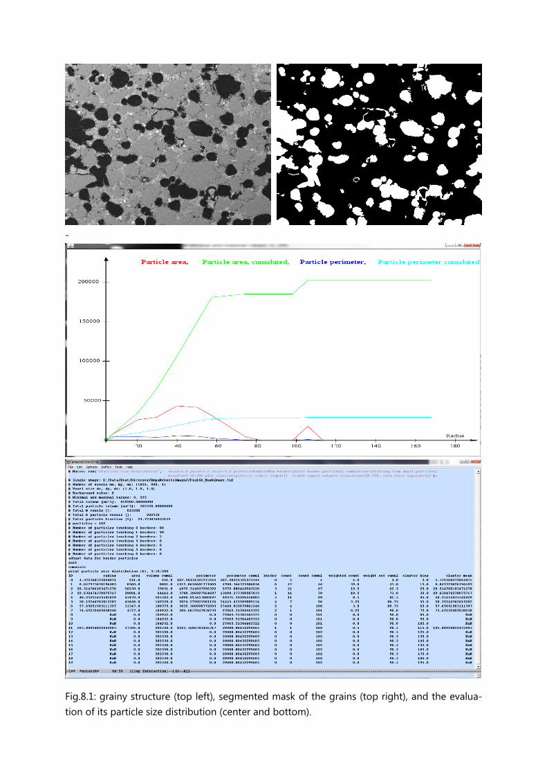
9.1 Particle Size Distribution This plugins calculates the particle size distribution (PSD) from a stack of images containing already segmented and labeled particles [15]. Either single images containing 2D particles, or stacks of images representing 3D volumes can be processed.

The following features can be calculated:

- particle ID - particle volume - cumulative particle volume - particle surface area - cumulative particle surface area - mean particle radius - number of particle borders - particle count - cumulative particle count - particle count weighted according to the number of boundaries - cumulative particle count weighted according to the number of boundaries - boundary value in case of clustering - cluster mean value in case of clustering

Correction of particles that are clipped at the borders is also possible. The correction is ap-plied to the resulting pore radii only (i.e. not for the pore volume). The plugin allows cumula-tive integration of the particle volumes and surfaces starting from either small or large parti-cles. The program plots out the resulting parameter fields.

Per default, the function plots a parameter set for each particle separately. Additionally, the program allows different types of clustering of the parameter sets. Clustering means sum-ming up or averaging the parameters within intervals yielding a histogram.

An example of a 2D particle image, of its mask and some particle evaluations is given in Fig. 8.1.

-

Fig.8.1: grainy structure (top left), segmented mask of the grains (top right), and the evalua-tion of its particle size distribution (center and bottom).

References:

15 - Münch B., Gasser P., Holzer L., Flatt R., "FIB Nanotomography of Particulate Systems - Part II: Particle Recognition and Effect of Boundary Truncation.", Journal American Ce-ramics Society 89(8), pp.2586-2595, 2006.

9.2 Phase Image Evaluation This plugins provides an evaluation of phase images [16, 17] containing labeled phases. For instance, labeled images might be created interactively with the help of the plugin "Segment Phases 3D", or even automatically with the plugin "Cluster Image".

The phase image evaluation calculates some parameters of all phases, including the percental phase contents and the phase areas. Additionally, mean image values for each phase can be provided, if one or more gray value images associated to the current phase image are pro-vided.

Furthermore, the plugin supports a peeling evaluation. Peeling starts from a specifically de-fined phase to its surroundings and requires a set of peeling radii defining toroidal regions around the starting phase. The peeling evaluation yields a data line at each peeling radius, including the peeling distance, number of pixels, mean value, and the percental phase con-tents for each phase. For image stacks, true 3D evaluations can be performed.

An image defining some phases is given in Fig.8.2 (top, left). The cyan colored center particle is supposed to act as the location from where peeling is initiated. The percental areas of the phases "Pores", "Matter", "Artificial" and "Unspecified" are plotted below. As it is evident from the calling parameters (Fig.8.2, top, right) two gray level data images associated to the pore mask are provided (center field). Their mean values depending on the peeling radius are displayed in the graph at the bottom. The parameters are provided in a text file as well (bottom).

Fig.8.2: phase image (top, left) and the parameters provided for the phase image evaluation (top, right). The resulting plots and the list of parameters are displayed below.

References:

16 - Leemann A., Münch B., Gasser P., Holzer L., "Influence of compaction on the interfacial transition zone and the permeability of concrete", Cement and Concrete Research 36, pp.1425-1433, 2006.

17 - Leemann A., Loser R., Münch B., "Influence of cement type on ITZ porosity and chloride resistance on self-compacting concrete", Cement & Concrete Composites 32, pp.116-120, 2010.

9.3 Pore Size Distribution This plugins calculates the pore size distribution (PSD) for a pore structure [18], i.e. the distri-bution of the pore radii. The PSD can be calculated either in 2D or in 3D if the program is running on a stack of images. The pore masks must be prepared beforehand such that a simple thresholding procedure is capable to separate the locations of the pore from the ma-terial. The PSD calculation will be running on the pore phase.

PDS's can be defined in different ways and must be chosen according to the specific requests [18]. The following PSD types can be calculated:

- Discrete PSD: the generally used definition of a PSD from image data. The pores are regarded as discrete object. At each single pore, its pore area or pore volume is cal-culated and the radius of its circle- or sphere-equivalent object given.

- Continuous PSD: the pore space is categorized into regions of different radii in the sense that the regions can be filled with balls of different radii. The sizes of those ra-dii are then attached to the respective locations. The histogram of radii then acts as continuous PSD.

- Continuous PSD with MIP simulation: same PSD definition as for the continuous PSD. However, the balls of different radii are intruded into the pore volume from one of the faces of the image cube (3D), or from one of the edges of the image (2D), respective-ly. This definition of the PSD corresponds to the pore size data that is retrieved by mercury intrusion porosimetry (MIP).

Fig.8.3 (top) shows a picture of a 3D volume of cement paste measured by FIB-nanotomography at a pixel size of 14.84 x 18.84 x 30.0 nm^3. The pores have been seg-mented by thresholding and different definitions of PSD's have been calculated in slice-wise 2D as well as in real 3D (bottom graph, containing the results of the PSD calculations visual-ized by Matlab).

Fig.8.3: 3D volume of cement paste (OPC CEM 1, 42.5, w/c 0.35, 28 days hydration) acquired by FIB-nanotomography (top) and its pore size distributions of varying definition (bottom, see ref.[18]).

References:

18 - Münch B., Holzer L., "Contradicting Geometrical Concepts in Pore Size Analysis Attained with Electron Microscopy and Mercury Intrusion", Journal of American Ceramics Society 91(12), pp.4059-4067, 2008.

10 Editors and Viewers This section contains plugins that are designed for user-interactive visualization and data processing on 2D slices and 3D volumes. They therefore don't just support a unique interac-tion on some image data, but they provide engines supporting an interactive dialog between the computer and the user.

10.1 Display Volume This plugin provides an orthogonal slicer for image volumes. The top view (xy), front view (xz) and side view (yz) of the volume are displayed at a specific point, the center point at startup. The point then can be moved by mouse interaction in one of the views while the remaining views keep track of the changes. Thereby, any x,y,z-location in the 3D volume can easily be focused and displayed. The image value at the current position is always plotted to the ImageJ window.

As an example, Fig.9.1 displays the view of the orthogonal slicer applied to the 3D volume displayed in Fig.8.3 (top). The red cross-lines of the slicer show the current 3D cursor posi-tion which allows interactively focusing any point in the 3D space. The position vector and the associated image value are plotted to the ImageJ window (top).

Fig.9.1: orthogonal slicer view of the 3D volume displayed in Fig. 8.3 (top).

10.2 Edit Label Region This plugin provides an engine for interactive editing of label images or label volumes (i.e. stacks of images). Label images are images holding a set of regions at one specific gray level or color per region (example see Fig.6.4, right). Operations such as deleting, joining, eroding, dilating, opening, or closing of manually selected 3D objects are supported. There is also an operation for deleting objects smaller than a certain size. For stacks of images, all operations can be performed either in slice-wise 2D, or truly volumetrically in 3D. The interface of the engine is visualized in Fig.9.2.

Fig.9.2: visualization of the interface for editing of labeled 3D regions.

10.3 Segment Phases 3D This plugin provides an engine for interactive segmentation of multiple phases. The program works on both, single images as well as image stacks. For image stacks, the operations can be performed in either slice-wise 2D or in 3D. All images or image stacks that are open in the current ImageJ session may serve as input images or image volumes. This benefit of being able to use multiple input images enables creating phase masks from multiple coincident or from multiple filtered versions of the same 2D or 3D scene.

The output of this program is a 2D phase image or a 3D phase stack of images which may contain up to 24 different phases. Each phase is created by defining a bit mask by using dif-ferent types of operations on any of the input images. Possible operations include manual drawing (by using the selection buttons on the ImageJ main toolbar), thresholding, regular or constrained region growing, erosion, dilation, and removal of small regions.

An intelligent workflow allows progressive refinement of each single phase represented by its bit mask. The bit masks are being interactively modified by using logical arithmetic (i.e. Bool-ean AND, OR, XOR, NOT) on a) the already present bit mask and b) the temporary mask cre-ated by one or more of the operations listed above. If, for instance, a thresholding operation was selected, its temporary mask can be added to the currently selected phase by running an "OR" operation.

A phase name and an ID are assessed to each phase for later processing. The ID is important in the case some phases may overlap each other, in order to define the priorities.

The resulting phase image or image stack is a 32-bit color TIFF image. All phase names and ID's are stored to the TIFF file header. Hence, a thereby created TIFF phase image can be re-loaded for further processing if required.

The segmentation engine is visualized in Fig.9.3 while operating on two SEM images of ce-ment paste (OPC CEM 1) acquired at the same location but at different microscope settings. The color image to the bottom right shows the currently constructed phase image consisting of 4 different overlapping phases. The same image in non-overlapping mode is displayed in Fig.8.2, top left. Currently, the phase named "Grain" is active and overlayed to the top left

gray level image in transparent blue. Like this, any current operation would now be achieved to the "Grain" phase. The rectangle and heart shapes were drawn manually with the selection tools.

Fig.9.3: engine for 3D segmentation "Segment Phases 3D" which is currently operating on two gray level images (left). The image at the bottom right is the interactively segmented phase image which is currently containing four different phases (see also Fig.8.2, top left).

10.4 View 3D Mask This plugin provides a 3D viewer of image and skeleton masks. The original data base should be a stack of images. An image mask may contain the mask of arbitrary objects, while skele-ton masks should contain objects which are previously skeletonized in 3D. 3D skeletoniza-tion can be performed by previously calling the "Skeletonization 2D 3D" plugin.

For 3D shading, the image masks can be either triangulated or voxelized. The triangulation is performed by using the well-known marching cubes algorithm [19], while voxelization is per-formed by a technique of Artzy et al [20].

The viewer is resizable. The 3D scene can be rotated, translated, or scaled. Rotation can be achieved with the left mouse button. Translation in x, y can be achieved by the right mouse button. Translation in z is sometimes useful if the viewer is too close to the

scene. It can be achieved by the middle mouse button. Scaling is achieved by simultaneous-ly pressing down the <shift> key and the left mouse button.

The current transform matrix is always stored to a text file located in the folder from where ImageJ was started. It is updated after each change of the rotation, translation or scaling. Like this, the current settings of the scene that seem to be useful for further visualizations can be stored to file.

The 3D viewer also contains a button to the bottom called "save canvas as JPEG". By pressing it, the current view can be stored to JPG image. The resolution of this image corresponds to the current resolution of the 3D window, i.e. to its window size.

As an example, a triangulated view of the segmented 3D volume (see Fig.8.3 (top) and Fig.9.1) is presented in Fig.9.4. Other examples were given in Fig.7.3.2 and in Fig.6.11 show-ing the original 3D scene (top), its skeleton (bottom left) and its skeleton after resizing its el-ements to their size determined by the distance transform values (see "Distance Transform" plugin).

Fig.9.4: triangulated and shaded visualization of the 3D volume in Fig.8.3 and Fig.9.1.

References:

19 - Lorensen W.E., Cline H.E., "Marching Cubes: a High Resolution 3D Surface Construction Algorithm", Computer Graphics 21(4), pp.163-169, 1987.

20 - Artzy E., Frieder G., Herman G.T., "The Theory, Design, Implementation and Evaluation of a Three-Dimensional Surface Detection Algorithm", Computer Graphics and Image Pro-cessing 15, pp.1-24, 1981.