Information Theory and Coding

Computer Science Tripos Part II, Michaelmas Term11 Lectures by J G Daugman

1. Foundations: Probability, Uncertainty, and Information

2. Entropies Defined, and Why they are Measures of Information

3. Source Coding Theorem; Prefix, Variable-, & Fixed-Length Codes

4. Channel Types, Properties, Noise, and Channel Capacity

5. Continuous Information; Density; Noisy Channel Coding Theorem

6. Fourier Series, Convergence, Orthogonal Representation

7. Useful Fourier Theorems; Transform Pairs; Sampling; Aliasing

8. Discrete Fourier Transform. Fast Fourier Transform Algorithms

9. The Quantized Degrees-of-Freedom in a Continuous Signal

10. Gabor-Heisenberg-Weyl Uncertainty Relation. Optimal “Logons”

11. Kolmogorov Complexity and Minimal Description Length

Information Theory and Coding

J G Daugman

Prerequisite courses: Probability; Mathematical Methods for CS; Discrete Mathematics

Aims

The aims of this course are to introduce the principles and applications of information theory.The course will study how information is measured in terms of probability and entropy, and therelationships among conditional and joint entropies; how these are used to calculate the capacityof a communication channel, with and without noise; coding schemes, including error correctingcodes; how discrete channels and measures of information generalise to their continuous forms;the Fourier perspective; and extensions to wavelets, complexity, compression, and efficient codingof audio-visual information.

Lectures

• Foundations: probability, uncertainty, information. How concepts of randomness,redundancy, compressibility, noise, bandwidth, and uncertainty are related to information.Ensembles, random variables, marginal and conditional probabilities. How the metrics ofinformation are grounded in the rules of probability.

• Entropies defined, and why they are measures of information. Marginal entropy,joint entropy, conditional entropy, and the Chain Rule for entropy. Mutual informationbetween ensembles of random variables. Why entropy is the fundamental measure of infor-mation content.

• Source coding theorem; prefix, variable-, and fixed-length codes. Symbol codes.The binary symmetric channel. Capacity of a noiseless discrete channel. Error correctingcodes.

• Channel types, properties, noise, and channel capacity. Perfect communicationthrough a noisy channel. Capacity of a discrete channel as the maximum of its mutualinformation over all possible input distributions.

• Continuous information; density; noisy channel coding theorem. Extensions of thediscrete entropies and measures to the continuous case. Signal-to-noise ratio; power spectraldensity. Gaussian channels. Relative significance of bandwidth and noise limitations. TheShannon rate limit and efficiency for noisy continuous channels.

• Fourier series, convergence, orthogonal representation. Generalised signal expan-sions in vector spaces. Independence. Representation of continuous or discrete data bycomplex exponentials. The Fourier basis. Fourier series for periodic functions. Examples.

• Useful Fourier theorems; transform pairs. Sampling; aliasing. The Fourier trans-form for non-periodic functions. Properties of the transform, and examples. Nyquist’sSampling Theorem derived, and the cause (and removal) of aliasing.

• Discrete Fourier transform. Fast Fourier Transform Algorithms. Efficient al-gorithms for computing Fourier transforms of discrete data. Computational complexity.Filters, correlation, modulation, demodulation, coherence.

• The quantised degrees-of-freedom in a continuous signal. Why a continuous sig-nal of finite bandwidth and duration has a fixed number of degrees-of-freedom. Diverseillustrations of the principle that information, even in such a signal, comes in quantised,countable, packets.

• Gabor-Heisenberg-Weyl uncertainty relation. Optimal “Logons”. Unification ofthe time-domain and the frequency-domain as endpoints of a continuous deformation. TheUncertainty Principle and its optimal solution by Gabor’s expansion basis of “logons”.Multi-resolution wavelet codes. Extension to images, for analysis and compression.

• Kolmogorov complexity. Minimal description length. Definition of the algorithmiccomplexity of a data sequence, and its relation to the entropy of the distribution fromwhich the data was drawn. Fractals. Minimal description length, and why this measure ofcomplexity is not computable.

Objectives

At the end of the course students should be able to

• calculate the information content of a random variable from its probability distribution

• relate the joint, conditional, and marginal entropies of variables in terms of their coupledprobabilities

• define channel capacities and properties using Shannon’s Theorems

• construct efficient codes for data on imperfect communication channels

• generalise the discrete concepts to continuous signals on continuous channels

• understand Fourier Transforms and the main ideas of efficient algorithms for them

• describe the information resolution and compression properties of wavelets

Recommended book

* Cover, T.M. & Thomas, J.A. (1991). Elements of information theory. New York: Wiley.

Information Theory and Coding

Computer Science Tripos Part II, Michaelmas Term

11 lectures by J G Daugman

1. Overview: What is Information Theory?

Key idea: The movements and transformations of information, just like

those of a fluid, are constrained by mathematical and physical laws.

These laws have deep connections with:

• probability theory, statistics, and combinatorics

• thermodynamics (statistical physics)

• spectral analysis, Fourier (and other) transforms

• sampling theory, prediction, estimation theory

• electrical engineering (bandwidth; signal-to-noise ratio)

• complexity theory (minimal description length)

• signal processing, representation, compressibility

As such, information theory addresses and answers the

two fundamental questions of communication theory:

1. What is the ultimate data compression?

(answer: the entropy of the data, H , is its compression limit.)

2. What is the ultimate transmission rate of communication?

(answer: the channel capacity, C, is its rate limit.)

All communication schemes lie in between these two limits on the com-

pressibility of data and the capacity of a channel. Information theory

can suggest means to achieve these theoretical limits. But the subject

also extends far beyond communication theory.

1

Important questions... to which Information Theory offers answers:

• How should information be measured?

• How much additional information is gained by some reduction in

uncertainty?

• How do the a priori probabilities of possible messages determine

the informativeness of receiving them?

• What is the information content of a random variable?

• How does the noise level in a communication channel limit its

capacity to transmit information?

• How does the bandwidth (in cycles/second) of a communication

channel limit its capacity to transmit information?

• By what formalism should prior knowledge be combined with

incoming data to draw formally justifiable inferences from both?

• How much information in contained in a strand of DNA?

• How much information is there in the firing pattern of a neurone?

Historical origins and important contributions:

• Ludwig BOLTZMANN (1844-1906), physicist, showed in 1877 that

thermodynamic entropy (defined as the energy of a statistical en-

semble [such as a gas] divided by its temperature: ergs/degree) is

related to the statistical distribution of molecular configurations,

with increasing entropy corresponding to increasing randomness. He

made this relationship precise with his famous formula S = k log W

where S defines entropy, W is the total number of possible molec-

ular configurations, and k is the constant which bears Boltzmann’s

name: k =1.38 x 10−16 ergs per degree centigrade. (The above

formula appears as an epitaph on Boltzmann’s tombstone.) This is

2

equivalent to the definition of the information (“negentropy”) in an

ensemble, all of whose possible states are equiprobable, but with a

minus sign in front (and when the logarithm is base 2, k=1.) The

deep connections between Information Theory and that branch of

physics concerned with thermodynamics and statistical mechanics,

hinge upon Boltzmann’s work.

• Leo SZILARD (1898-1964) in 1929 identified entropy with informa-

tion. He formulated key information-theoretic concepts to solve the

thermodynamic paradox known as “Maxwell’s demon” (a thought-

experiment about gas molecules in a partitioned box) by showing

that the amount of information required by the demon about the

positions and velocities of the molecules was equal (negatively) to

the demon’s entropy increment.

• James Clerk MAXWELL (1831-1879) originated the paradox called

“Maxwell’s Demon” which greatly influenced Boltzmann and which

led to the watershed insight for information theory contributed by

Szilard. At Cambridge, Maxwell founded the Cavendish Laboratory

which became the original Department of Physics.

• R V HARTLEY in 1928 founded communication theory with his

paper Transmission of Information. He proposed that a signal

(or a communication channel) having bandwidth Ω over a duration

T has a limited number of degrees-of-freedom, namely 2ΩT , and

therefore it can communicate at most this quantity of information.

He also defined the information content of an equiprobable ensemble

of N possible states as equal to log2 N .

• Norbert WIENER (1894-1964) unified information theory and Fourier

analysis by deriving a series of relationships between the two. He

invented “white noise analysis” of non-linear systems, and made the

definitive contribution to modeling and describing the information

content of stochastic processes known as Time Series.

3

• Dennis GABOR (1900-1979) crystallized Hartley’s insight by formu-

lating a general Uncertainty Principle for information, expressing

the trade-off for resolution between bandwidth and time. (Signals

that are well specified in frequency content must be poorly localized

in time, and those that are well localized in time must be poorly

specified in frequency content.) He formalized the “Information Di-

agram” to describe this fundamental trade-off, and derived the con-

tinuous family of functions which optimize (minimize) the conjoint

uncertainty relation. In 1974 Gabor won the Nobel Prize in Physics

for his work in Fourier optics, including the invention of holography.

• Claude SHANNON (together with Warren WEAVER) in 1949 wrote

the definitive, classic, work in information theory: Mathematical

Theory of Communication. Divided into separate treatments for

continuous-time and discrete-time signals, systems, and channels,

this book laid out all of the key concepts and relationships that de-

fine the field today. In particular, he proved the famous Source Cod-

ing Theorem and the Noisy Channel Coding Theorem, plus many

other related results about channel capacity.

• S KULLBACK and R A LEIBLER (1951) defined relative entropy

(also called information for discrimination, or K-L Distance.)

• E T JAYNES (since 1957) developed maximum entropy methods

for inference, hypothesis-testing, and decision-making, based on the

physics of statistical mechanics. Others have inquired whether these

principles impose fundamental physical limits to computation itself.

• A N KOLMOGOROV in 1965 proposed that the complexity of a

string of data can be defined by the length of the shortest binary

program for computing the string. Thus the complexity of data

is its minimal description length, and this specifies the ultimate

compressibility of data. The “Kolmogorov complexity” K of a string

is approximately equal to its Shannon entropy H , thereby unifying

the theory of descriptive complexity and information theory.

4

2. Mathematical Foundations; Probability Rules;

Bayes’ Theorem

What are random variables? What is probability?

Random variables are variables that take on values determined by prob-

ability distributions. They may be discrete or continuous, in either their

domain or their range. For example, a stream of ASCII encoded text

characters in a transmitted message is a discrete random variable, with

a known probability distribution for any given natural language. An

analog speech signal represented by a voltage or sound pressure wave-

form as a function of time (perhaps with added noise), is a continuous

random variable having a continuous probability density function.

Most of Information Theory involves probability distributions of ran-

dom variables, and conjoint or conditional probabilities defined over

ensembles of random variables. Indeed, the information content of a

symbol or event is defined by its (im)probability. Classically, there are

two different points of view about what probability actually means:

• relative frequency: sample the random variable a great many times

and tally up the fraction of times that each of its different possible

values occurs, to arrive at the probability of each.

• degree-of-belief: probability is the plausibility of a proposition or

the likelihood that a particular state (or value of a random variable)

might occur, even if its outcome can only be decided once (e.g. the

outcome of a particular horse-race).

The first view, the “frequentist” or operationalist view, is the one that

predominates in statistics and in information theory. However, by no

means does it capture the full meaning of probability. For example,

the proposition that "The moon is made of green cheese" is one

which surely has a probability that we should be able to attach to it.

We could assess its probability by degree-of-belief calculations which

5

combine our prior knowledge about physics, geology, and dairy prod-

ucts. Yet the “frequentist” definition of probability could only assign

a probability to this proposition by performing (say) a large number

of repeated trips to the moon, and tallying up the fraction of trips on

which the moon turned out to be a dairy product....

In either case, it seems sensible that the less probable an event is, the

more information is gained by noting its occurrence. (Surely discovering

that the moon IS made of green cheese would be more “informative”

than merely learning that it is made only of earth-like rocks.)

Probability Rules

Most of probability theory was laid down by theologians: Blaise PAS-

CAL (1623-1662) who gave it the axiomatization that we accept today;

and Thomas BAYES (1702-1761) who expressed one of its most impor-

tant and widely-applied propositions relating conditional probabilities.

Probability Theory rests upon two rules:

Product Rule:

p(A, B) = “joint probability of both A and B”

= p(A|B)p(B)

or equivalently,

= p(B|A)p(A)

Clearly, in case A and B are independent events, they are not condi-

tionalized on each other and so

p(A|B) = p(A)

and p(B|A) = p(B),

in which case their joint probability is simply p(A, B) = p(A)p(B).

6

Sum Rule:

If event A is conditionalized on a number of other events B, then the

total probability of A is the sum of its joint probabilities with all B:

p(A) =∑

Bp(A, B) =

∑

Bp(A|B)p(B)

From the Product Rule and the symmetry that p(A, B) = p(B, A), it

is clear that p(A|B)p(B) = p(B|A)p(A). Bayes’ Theorem then follows:

Bayes’ Theorem:

p(B|A) =p(A|B)p(B)

p(A)

The importance of Bayes’ Rule is that it allows us to reverse the condi-

tionalizing of events, and to compute p(B|A) from knowledge of p(A|B),

p(A), and p(B). Often these are expressed as prior and posterior prob-

abilities, or as the conditionalizing of hypotheses upon data.

Worked Example:

Suppose that a dread disease affects 1/1000th of all people. If you ac-

tually have the disease, a test for it is positive 95% of the time, and

negative 5% of the time. If you don’t have the disease, the test is posi-

tive 5% of the time. We wish to know how to interpret test results.

Suppose you test positive for the disease. What is the likelihood that

you actually have it?

We use the above rules, with the following substitutions of “data” D

and “hypothesis” H instead of A and B:

D = data: the test is positive

H = hypothesis: you have the disease

H = the other hypothesis: you do not have the disease

7

Before acquiring the data, we know only that the a priori probabil-

ity of having the disease is .001, which sets p(H). This is called a prior.

We also need to know p(D).

From the Sum Rule, we can calculate that the a priori probability

p(D) of testing positive, whatever the truth may actually be, is:

p(D) = p(D|H)p(H) + p(D|H)p(H) =(.95)(.001)+(.05)(.999) = .051

and from Bayes’ Rule, we can conclude that the probability that you

actually have the disease given that you tested positive for it, is much

smaller than you may have thought:

p(H|D) =p(D|H)p(H)

p(D)=

(.95)(.001)

(.051)= 0.019 (less than 2%).

This quantity is called the posterior probability because it is computed

after the observation of data; it tells us how likely the hypothesis is,

given what we have observed. (Note: it is an extremely common human

fallacy to confound p(H|D) with p(D|H). In the example given, most

people would react to the positive test result by concluding that the

likelihood that they have the disease is .95, since that is the “hit rate”

of the test. They confound p(D|H) = .95 with p(H|D) = .019, which

is what actually matters.)

A nice feature of Bayes’ Theorem is that it provides a simple mech-

anism for repeatedly updating our assessment of the hypothesis as more

data continues to arrive. We can apply the rule recursively, using the

latest posterior as the new prior for interpreting the next set of data.

In Artificial Intelligence, this feature is important because it allows the

systematic and real-time construction of interpretations that can be up-

dated continuously as more data arrive in a time series, such as a flow

of images or spoken sounds that we wish to understand.

8

3. Entropies Defined, and Why They are

Measures of Information

The information content I of a single event or message is defined as the

base-2 logarithm of its probability p:

I = log2 p (1)

and its entropy H is considered the negative of this. Entropy can be

regarded intuitively as “uncertainty,” or “disorder.” To gain information

is to lose uncertainty by the same amount, so I and H differ only in

sign (if at all): H = −I. Entropy and information have units of bits.

Note that I as defined in Eqt (1) is never positive: it ranges between

0 and −∞ as p varies from 1 to 0. However, sometimes the sign is

dropped, and I is considered the same thing as H (as we’ll do later too).

No information is gained (no uncertainty is lost) by the appearance

of an event or the receipt of a message that was completely certain any-

way (p = 1, so I = 0). Intuitively, the more improbable an event is,

the more informative it is; and so the monotonic behaviour of Eqt (1)

seems appropriate. But why the logarithm?

The logarithmic measure is justified by the desire for information to

be additive. We want the algebra of our measures to reflect the Rules

of Probability. When independent packets of information arrive, we

would like to say that the total information received is the sum of

the individual pieces. But the probabilities of independent events

multiply to give their combined probabilities, and so we must take

logarithms in order for the joint probability of independent events

or messages to contribute additively to the information gained.

This principle can also be understood in terms of the combinatorics

of state spaces. Suppose we have two independent problems, one with n

9

possible solutions (or states) each having probability pn, and the other

with m possible solutions (or states) each having probability pm. Then

the number of combined states is mn, and each of these has probability

pmpn. We would like to say that the information gained by specifying

the solution to both problems is the sum of that gained from each one.

This desired property is achieved:

Imn = log2(pmpn) = log2 pm + log2 pn = Im + In (2)

A Note on Logarithms:

In information theory we often wish to compute the base-2 logarithms

of quantities, but most calculators (and tools like xcalc) only offer

Napierian (base 2.718...) and decimal (base 10) logarithms. So the

following conversions are useful:

log2 X = 1.443 loge X = 3.322 log10 X

Henceforward we will omit the subscript; base-2 is always presumed.

Intuitive Example of the Information Measure (Eqt 1):

Suppose I choose at random one of the 26 letters of the alphabet, and we

play the game of “25 questions” in which you must determine which let-

ter I have chosen. I will only answer ‘yes’ or ‘no.’ What is the minimum

number of such questions that you must ask in order to guarantee find-

ing the answer? (What form should such questions take? e.g., “Is it A?”

“Is it B?” ...or is there some more intelligent way to solve this problem?)

The answer to a Yes/No question having equal probabilities conveys

one bit worth of information. In the above example with equiprobable

states, you never need to ask more than 5 (well-phrased!) questions to

discover the answer, even though there are 26 possibilities. Appropri-

ately, Eqt (1) tells us that the uncertainty removed as a result of solving

this problem is about -4.7 bits.

10

Entropy of Ensembles

We now move from considering the information content of a single event

or message, to that of an ensemble. An ensemble is the set of outcomes

of one or more random variables. The outcomes have probabilities at-

tached to them. In general these probabilities are non-uniform, with

event i having probability pi, but they must sum to 1 because all possi-

ble outcomes are included; hence they form a probability distribution:

∑

ipi = 1 (3)

The entropy of an ensemble is simply the average entropy of all the

elements in it. We can compute their average entropy by weighting each

of the log pi contributions by its probability pi:

H = −I = −∑

ipi log pi (4)

Eqt (4) allows us to speak of the information content or the entropy of

a random variable, from knowledge of the probability distribution that

it obeys. (Entropy does not depend upon the actual values taken by

the random variable! – Only upon their relative probabilities.)

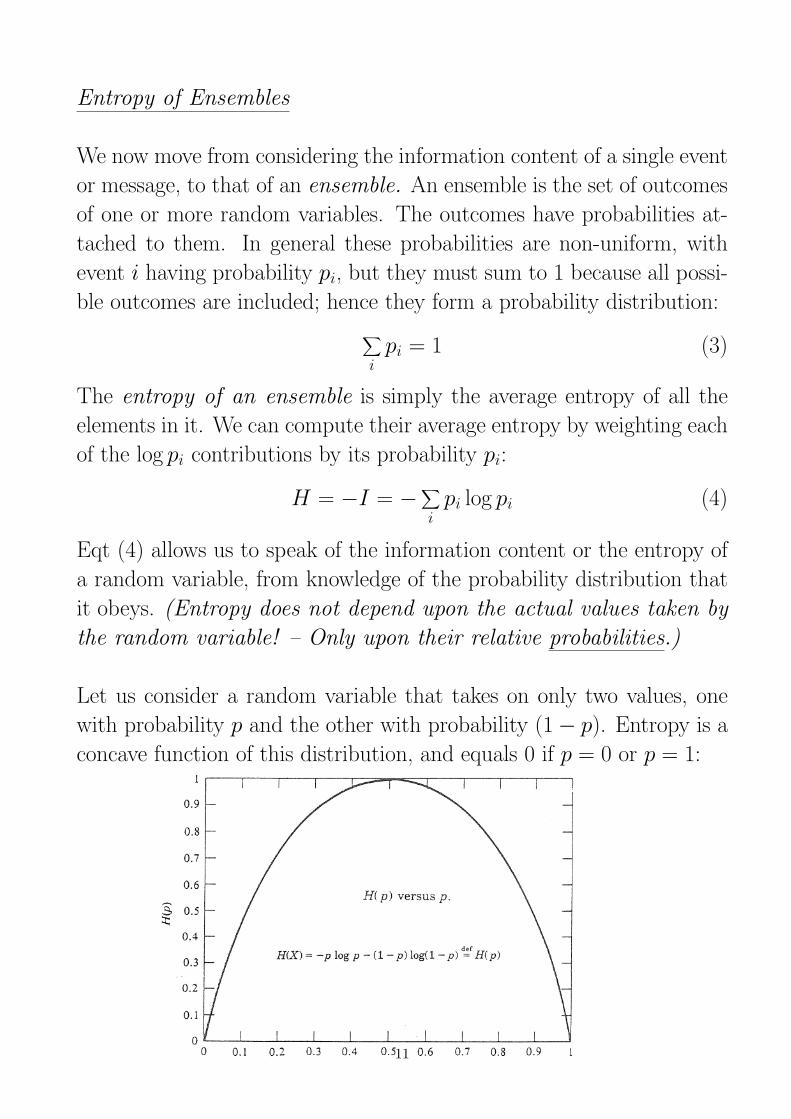
Let us consider a random variable that takes on only two values, one

with probability p and the other with probability (1 − p). Entropy is a

concave function of this distribution, and equals 0 if p = 0 or p = 1:

11

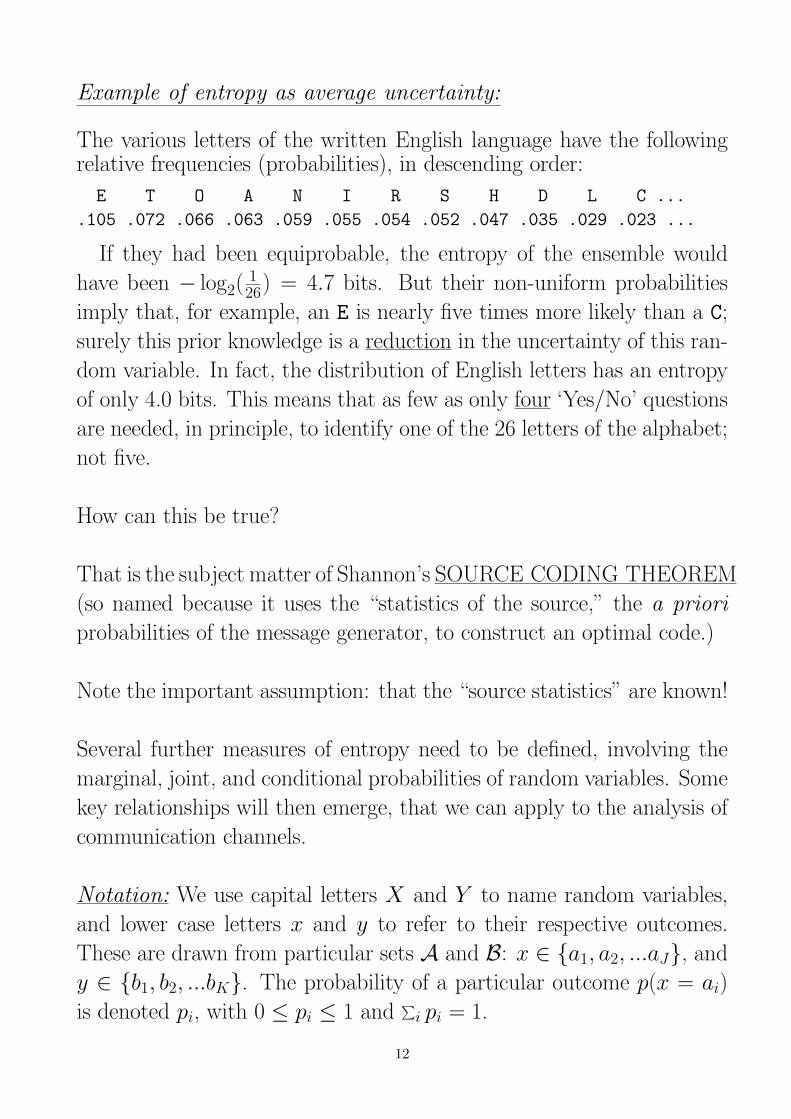
Example of entropy as average uncertainty:

The various letters of the written English language have the followingrelative frequencies (probabilities), in descending order:

E T O A N I R S H D L C ...

.105 .072 .066 .063 .059 .055 .054 .052 .047 .035 .029 .023 ...

If they had been equiprobable, the entropy of the ensemble would

have been − log2(126) = 4.7 bits. But their non-uniform probabilities

imply that, for example, an E is nearly five times more likely than a C;

surely this prior knowledge is a reduction in the uncertainty of this ran-

dom variable. In fact, the distribution of English letters has an entropy

of only 4.0 bits. This means that as few as only four ‘Yes/No’ questions

are needed, in principle, to identify one of the 26 letters of the alphabet;

not five.

How can this be true?

That is the subject matter of Shannon’s SOURCE CODING THEOREM

(so named because it uses the “statistics of the source,” the a priori

probabilities of the message generator, to construct an optimal code.)

Note the important assumption: that the “source statistics” are known!

Several further measures of entropy need to be defined, involving the

marginal, joint, and conditional probabilities of random variables. Some

key relationships will then emerge, that we can apply to the analysis of

communication channels.

Notation: We use capital letters X and Y to name random variables,

and lower case letters x and y to refer to their respective outcomes.

These are drawn from particular sets A and B: x ∈ a1, a2, ...aJ, and

y ∈ b1, b2, ...bK. The probability of a particular outcome p(x = ai)

is denoted pi, with 0 ≤ pi ≤ 1 and∑

i pi = 1.

12

An ensemble is just a random variable X , whose entropy was defined

in Eqt (4). A joint ensemble ‘XY ’ is an ensemble whose outcomes

are ordered pairs x, y with x ∈ a1, a2, ...aJ and y ∈ b1, b2, ...bK.The joint ensemble XY defines a probability distribution p(x, y) over

all possible joint outcomes x, y.

Marginal probability: From the Sum Rule, we can see that the proba-

bility of X taking on a particular value x = ai is the sum of the joint

probabilities of this outcome for X and all possible outcomes for Y :

p(x = ai) =∑

yp(x = ai, y)

We can simplify this notation to: p(x) =∑

yp(x, y)

and similarly: p(y) =∑

xp(x, y)

Conditional probability: From the Product Rule, we can easily see that

the conditional probability that x = ai, given that y = bj, is:

p(x = ai|y = bj) =p(x = ai, y = bj)

p(y = bj)

We can simplify this notation to: p(x|y) =p(x, y)

p(y)

and similarly: p(y|x) =p(x, y)

p(x)

It is now possible to define various entropy measures for joint ensembles:

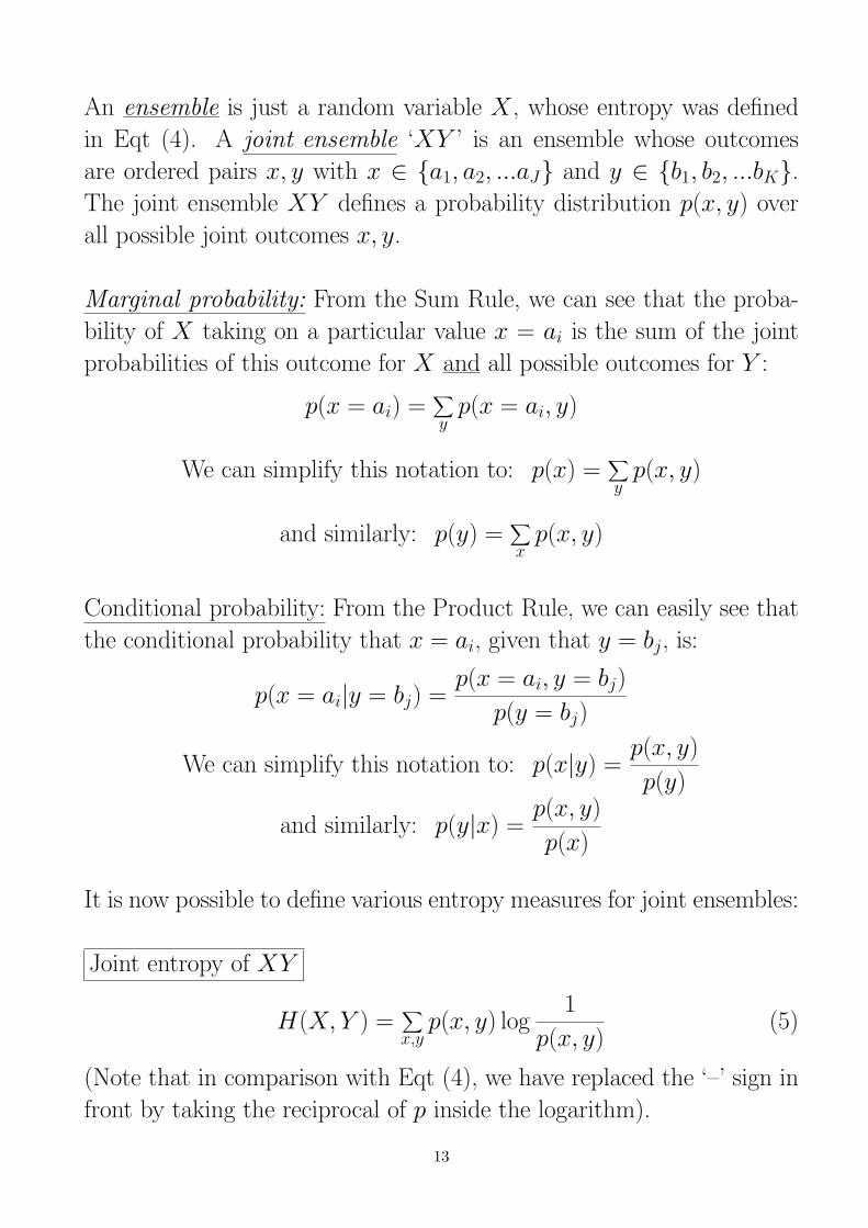
Joint entropy of XY

H(X, Y ) =∑

x,yp(x, y) log

1

p(x, y)(5)

(Note that in comparison with Eqt (4), we have replaced the ‘–’ sign in

front by taking the reciprocal of p inside the logarithm).

13

From this definition, it follows that joint entropy is additive if X and Y

are independent random variables:

H(X, Y ) = H(X) + H(Y ) iff p(x, y) = p(x)p(y)

Prove this.

Conditional entropy of an ensemble X , given that y = bj

measures the uncertainty remaining about random variable X after

specifying that random variable Y has taken on a particular value

y = bj. It is defined naturally as the entropy of the probability dis-

tribution p(x|y = bj):

H(X|y = bj) =∑

xp(x|y = bj) log

1

p(x|y = bj)(6)

If we now consider the above quantity averaged over all possible out-

comes that Y might have, each weighted by its probability p(y), then

we arrive at the...

Conditional entropy of an ensemble X , given an ensemble Y :

H(X|Y ) =∑

yp(y)

∑

xp(x|y) log

1

p(x|y)

(7)

and we know from the Sum Rule that if we move the p(y) term from

the outer summation over y, to inside the inner summation over x, the

two probability terms combine and become just p(x, y) summed over all

x, y. Hence a simpler expression for this conditional entropy is:

H(X|Y ) =∑

x,yp(x, y) log

1

p(x|y)(8)

This measures the average uncertainty that remains about X , when Y

is known.

14

Chain Rule for Entropy

The joint entropy, conditional entropy, and marginal entropy for two

ensembles X and Y are related by:

H(X, Y ) = H(X) + H(Y |X) = H(Y ) + H(X|Y ) (9)

It should seem natural and intuitive that the joint entropy of a pair of

random variables is the entropy of one plus the conditional entropy of

the other (the uncertainty that it adds once its dependence on the first

one has been discounted by conditionalizing on it). You can derive the

Chain Rule from the earlier definitions of these three entropies.

Corollary to the Chain Rule:

If we have three random variables X, Y, Z, the conditionalizing of the

joint distribution of any two of them, upon the third, is also expressed

by a Chain Rule:

H(X, Y |Z) = H(X|Z) + H(Y |X, Z) (10)

“Independence Bound on Entropy”

A consequence of the Chain Rule for Entropy is that if we have many

different random variables X1, X2, ..., Xn, then the sum of all their in-

dividual entropies is an upper bound on their joint entropy:

H(X1, X2, ..., Xn) ≤n

∑

i=1H(Xi) (11)

Their joint entropy only reaches this upper bound if all of the random

variables are independent.

15

Mutual Information between X and Y

The mutual information between two random variables measures the

amount of information that one conveys about the other. Equivalently,

it measures the average reduction in uncertainty about X that results

from learning about Y . It is defined:

I(X ; Y ) =∑

x,yp(x, y) log

p(x, y)

p(x)p(y)(12)

Clearly X says as much about Y as Y says about X . Note that in case

X and Y are independent random variables, then the numerator inside

the logarithm equals the denominator. Then the log term vanishes, and

the mutual information equals zero, as one should expect.

Non-negativity: mutual information is always ≥ 0. In the event that

the two random variables are perfectly correlated, then their mutual

information is the entropy of either one alone. (Another way to say

this is: I(X ; X) = H(X): the mutual information of a random vari-

able with itself is just its entropy. For this reason, the entropy H(X)

of a random variable X is sometimes referred to as its self-information.)

These properties are reflected in three equivalent definitions for the mu-

tual information between X and Y :

I(X ; Y ) = H(X) − H(X|Y ) (13)

I(X ; Y ) = H(Y ) − H(Y |X) = I(Y ; X) (14)

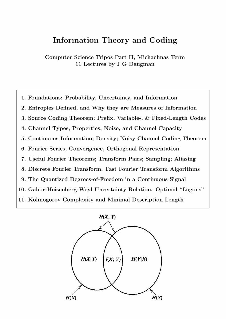
I(X ; Y ) = H(X) + H(Y ) − H(X, Y ) (15)

In a sense the mutual information I(X ; Y ) is the intersection between

H(X) and H(Y ), since it represents their statistical dependence. In the

Venn diagram given at the top of page 18, the portion of H(X) that

does not lie within I(X ; Y ) is just H(X|Y ). The portion of H(Y ) that

does not lie within I(X ; Y ) is just H(Y |X).

16

Distance D(X, Y ) between X and Y

The amount by which the joint entropy of two random variables ex-

ceeds their mutual information is a measure of the “distance” between

them:

D(X, Y ) = H(X, Y ) − I(X ; Y ) (16)

Note that this quantity satisfies the standard axioms for a distance:

D(X, Y ) ≥ 0, D(X, X) = 0, D(X, Y ) = D(Y, X), and

D(X, Z) ≤ D(X, Y ) + D(Y, Z).

Relative entropy, or Kullback-Leibler distance

Another important measure of the “distance” between two random vari-

ables, although it does not satisfy the above axioms for a distance metric,

is the relative entropy or Kullback-Leibler distance. It is also called

the information for discrimination. If p(x) and q(x) are two proba-

bility distributions defined over the same set of outcomes x, then their

relative entropy is:

DKL(p‖q) =∑

xp(x) log

p(x)

q(x)(17)

Note that DKL(p‖q) ≥ 0, and in case p(x) = q(x) then their distance

DKL(p‖q) = 0, as one might hope. However, this metric is not strictly a

“distance,” since in general it lacks symmetry: DKL(p‖q) 6= DKL(q‖p).

The relative entropy DKL(p‖q) is a measure of the “inefficiency” of as-

suming that a distribution is q(x) when in fact it is p(x). If we have an

optimal code for the distribution p(x) (meaning that we use on average

H(p(x)) bits, its entropy, to describe it), then the number of additional

bits that we would need to use if we instead described p(x) using an

optimal code for q(x), would be their relative entropy DKL(p‖q).

17

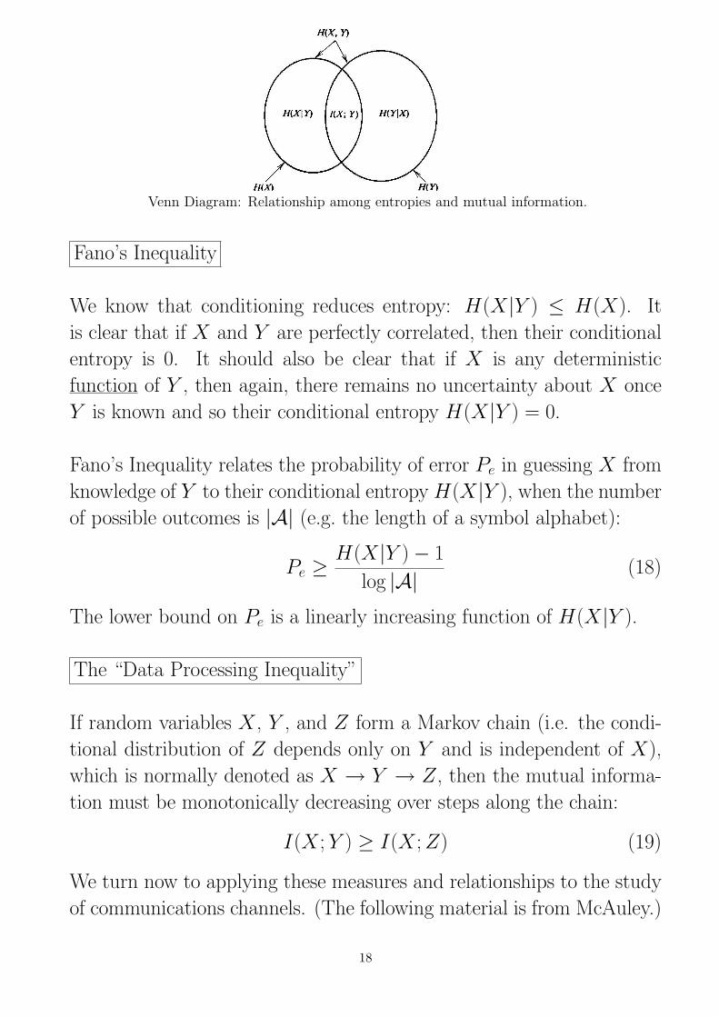
Venn Diagram: Relationship among entropies and mutual information.

Fano’s Inequality

We know that conditioning reduces entropy: H(X|Y ) ≤ H(X). It

is clear that if X and Y are perfectly correlated, then their conditional

entropy is 0. It should also be clear that if X is any deterministic

function of Y , then again, there remains no uncertainty about X once

Y is known and so their conditional entropy H(X|Y ) = 0.

Fano’s Inequality relates the probability of error Pe in guessing X from

knowledge of Y to their conditional entropy H(X|Y ), when the number

of possible outcomes is |A| (e.g. the length of a symbol alphabet):

Pe ≥H(X|Y ) − 1

log |A| (18)

The lower bound on Pe is a linearly increasing function of H(X|Y ).

The “Data Processing Inequality”

If random variables X , Y , and Z form a Markov chain (i.e. the condi-

tional distribution of Z depends only on Y and is independent of X),

which is normally denoted as X → Y → Z, then the mutual informa-

tion must be monotonically decreasing over steps along the chain:

I(X ; Y ) ≥ I(X ; Z) (19)

We turn now to applying these measures and relationships to the study

of communications channels. (The following material is from McAuley.)

18

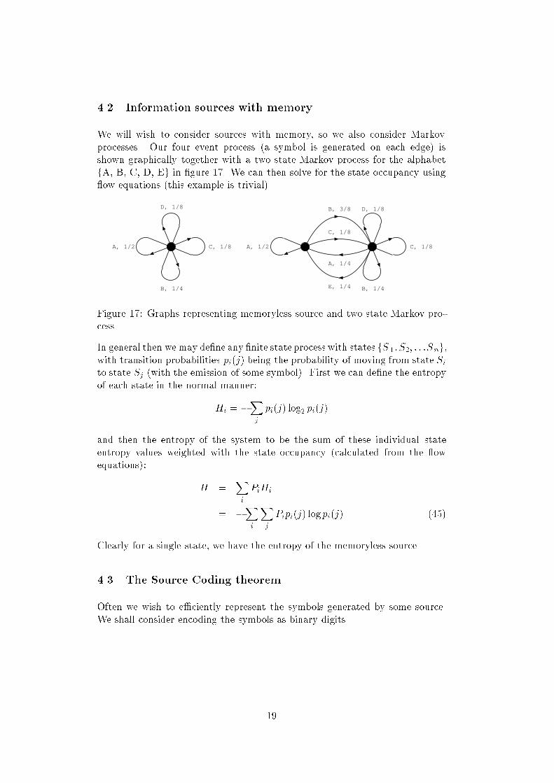
4.2 Information sources with memoryWe will wish to consider sources with memory, so we also consider Markovprocesses. Our four event process (a symbol is generated on each edge) isshown graphically together with a two state Markov process for the alphabetfA, B, C, D, Eg in gure 17. We can then solve for the state occupancy using ow equations (this example is trivial).D, 1/8

C, 1/8

B, 1/4

A, 1/2 A, 1/2

B, 3/8

C, 1/8

D, 1/8

B, 1/4

C, 1/8

A, 1/4

E, 1/4Figure 17: Graphs representing memoryless source and two state Markov pro-cessIn general then we may dene any nite state process with states fS 1; S2; : : :Sng,with transition probabilities pi(j) being the probability of moving from state Sito state Sj (with the emission of some symbol). First we can dene the entropyof each state in the normal manner:Hi = Xj pi(j) log2 pi(j)and then the entropy of the system to be the sum of these individual stateentropy values weighted with the state occupancy (calculated from the owequations): H = Xi PiHi= Xi Xj Pipi(j) logpi(j) (45)Clearly for a single state, we have the entropy of the memoryless source.4.3 The Source Coding theoremOften we wish to eciently represent the symbols generated by some source.We shall consider encoding the symbols as binary digits.19

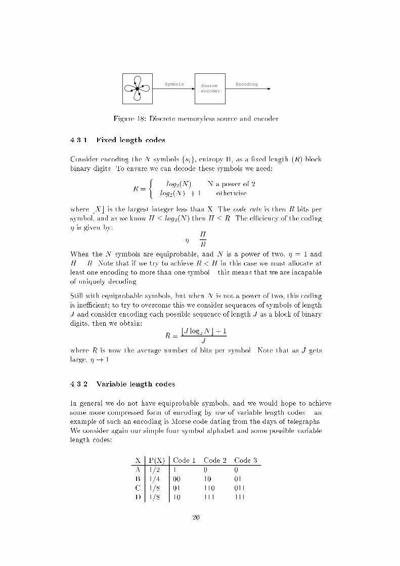
Symbols EncodingSourceencoderFigure 18: Discrete memoryless source and encoder4.3.1 Fixed length codesConsider encoding the N symbols fsig, entropy H, as a xed length (R) blockbinary digits. To ensure we can decode these symbols we need:R = ( log2(N) N a power of 2blog2(N)c+ 1 otherwisewhere bXc is the largest integer less than X. The code rate is then R bits persymbol, and as we know H log2(N) then H R. The eciency of the coding is given by: = HRWhen the N symbols are equiprobable, and N is a power of two, = 1 andH = R. Note that if we try to achieve R < H in this case we must allocate atleast one encoding to more than one symbol this means that we are incapableof uniquely decoding.Still with equiprobable symbols, but when N is not a power of two, this codingis inecient; to try to overcome this we consider sequences of symbols of lengthJ and consider encoding each possible sequence of length J as a block of binarydigits, then we obtain: R = bJ log2Nc+ 1Jwhere R is now the average number of bits per symbol. Note that as J getslarge, ! 1.4.3.2 Variable length codesIn general we do not have equiprobable symbols, and we would hope to achievesome more compressed form of encoding by use of variable length codes anexample of such an encoding is Morse code dating from the days of telegraphs.We consider again our simple four symbol alphabet and some possible variablelength codes: X P(X) Code 1 Code 2 Code 3A 1=2 1 0 0B 1=4 00 10 01C 1=8 01 110 011D 1=8 10 111 11120

We consider each code in turn:1. Using this encoding, we nd that presented with a sequence like 1001, wedo not know whether to decode as ABA or DC. This makes such a codeunsatisfactory. Further, in general, even a code where such an ambiguitycould be resolved uniquely by looking at bits further ahead in the stream(and backtracking) is unsatisfactory.Observe that for this code, the coding rate, or average number of bits persymbol, is given by:Pi sibi = 12 1 + 14 2 + 2 18 2= 32which is less than the entropy.2. This code is uniquely decodable; further this code is interesting in thatwe can decode instantaneously that is no backtracking is required; oncewe have the bits of the encoded symbol we can decode without waitingfor more. Further this also satises the prex condition, that is there isno code word which is prex (i.e. same bit pattern) of a longer code word.In this case the coding rate is equal to the entropy.3. While this is de-codable (and coding rate is equal to the entropy again),observe that it does not have the prex property and is not an instanta-neous code.Shannon's rst theorem is the source-coding theorem which is:For a discrete memoryless source with nite entropy H ; for any(positive) it is possible to encode the symbols at an average rateR, such that: R = H + (For proof see Shannon & Weaver.) This is also sometimes called the noiselesscoding theorem as it deals with coding without consideration of noise processes(i.e. bit corruption etc).The entropy function then represents a fundamental limit on the number of bitson average required to represent the symbols of the source.4.3.3 Prex codesWe have already mentioned the prex property; we nd that for a prex codeto exist, it must satisfy the Kraft-McMillan inequality. That is,a necessary (notsucient) condition for a code having binary code words with length n1 n2 nN to satisfy the prex condition is:NXi=1 12ni 121

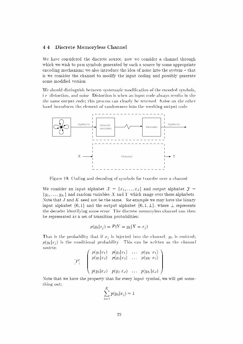
4.4 Discrete Memoryless ChannelWe have considered the discrete source, now we consider a channel throughwhich we wish to pass symbols generated by such a source by some appropriateencoding mechanism; we also introduce the idea of noise into the system thatis we consider the channel to modify the input coding and possibly generatesome modied version.We should distinguish between systematic modication of the encoded symbols,i.e. distortion, and noise. Distortion is when an input code always results in thethe same output code; this process can clearly be reversed. Noise on the otherhand introduces the element of randomness into the resulting output code.Symbols Source

encoder DecoderSymbols

ChannelX YFigure 19: Coding and decoding of symbols for transfer over a channel.We consider an input alphabet X = fx1; : : : ; xJg and output alphabet Y =fy1; : : : ; yKg and random variables X and Y which range over these alphabets.Note that J and K need not be the same for example we may have the binaryinput alphabet f0; 1g and the output alphabet f0; 1;?g, where ? representsthe decoder identifying some error. The discrete memoryless channel can thenbe represented as a set of transition probabilities:p(ykjxj) = P (Y = ykjX = xj)That is the probability that if xj is injected into the channel, yk is emitted;p(ykjxj) is the conditional probability. This can be written as the channelmatrix: [P ] = 0BBBB@ p(y1jx1) p(y2jx1) : : : p(yK jx1)p(y1jx2) p(y2jx2) : : : p(yK jx2)... ... . . . ...p(y1jxJ) p(y2jxJ) : : : p(yK jxJ) 1CCCCANote that we have the property that for every input symbol, we will get some-thing out: KXk=1 p(ykjxj) = 122

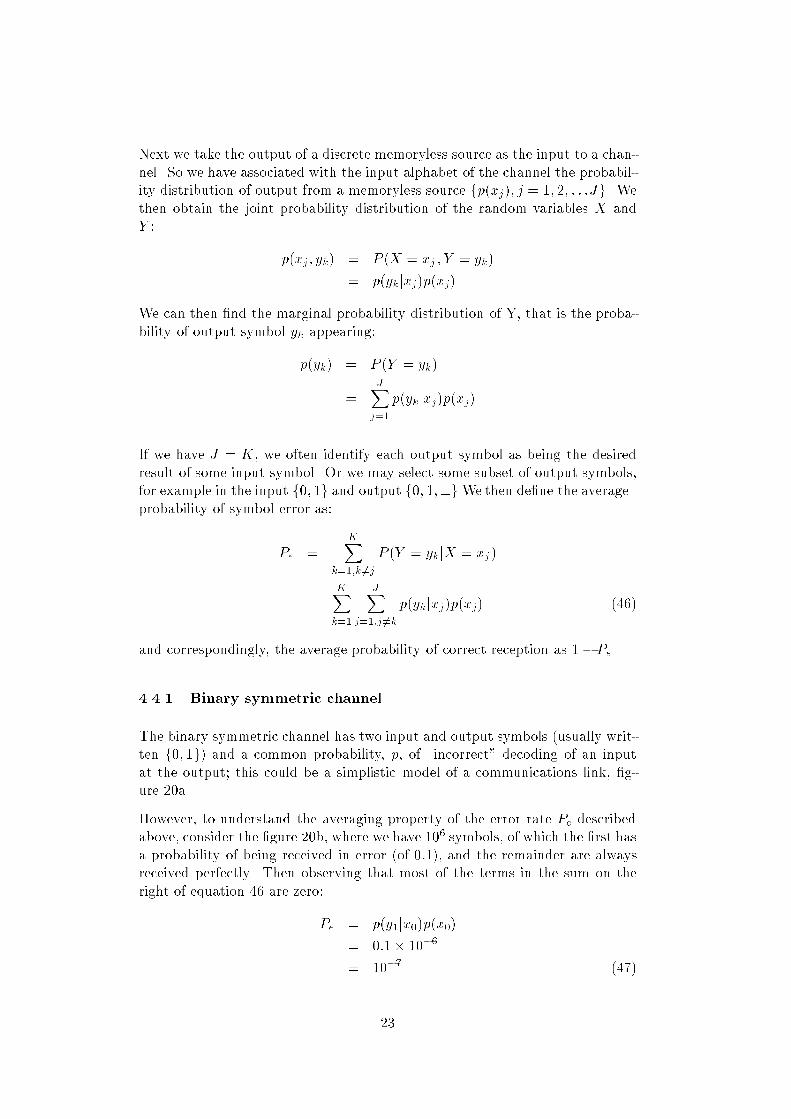
Next we take the output of a discrete memoryless source as the input to a chan-nel. So we have associated with the input alphabet of the channel the probabil-ity distribution of output from a memoryless source fp(xj); j = 1; 2; : : :Jg. Wethen obtain the joint probability distribution of the random variables X andY : p(xj ; yk) = P (X = xj ; Y = yk)= p(ykjxj)p(xj)We can then nd the marginal probability distribution of Y, that is the proba-bility of output symbol yk appearing:p(yk) = P (Y = yk)= JXj=1 p(ykjxj)p(xj)If we have J = K, we often identify each output symbol as being the desiredresult of some input symbol. Or we may select some subset of output symbols,for example in the input f0; 1g and output f0; 1;?g.We then dene the averageprobability of symbol error as:Pe = KXk=1;k 6=j P (Y = yk jX = xj )= KXk=1 JXj=1;j 6=k p(yk jxj)p(xj) (46)and correspondingly, the average probability of correct reception as 1 Pe.4.4.1 Binary symmetric channelThe binary symmetric channel has two input and output symbols (usually writ-ten f0; 1g) and a common probability, p, of \incorrect" decoding of an inputat the output; this could be a simplistic model of a communications link, g-ure 20a.However, to understand the averaging property of the error rate Pe describedabove, consider the gure 20b, where we have 106 symbols, of which the rst hasa probability of being received in error (of 0:1), and the remainder are alwaysreceived perfectly. Then observing that most of the terms in the sum on theright of equation 46 are zero:Pe = p(y1jx0)p(x0)= 0:1 106= 107 (47)23

0

11

0

p

p

1-p

1-p

X Y

0

11

0

YX

0.1

0.9

1.0

1.0

1.0

2

3

2

3

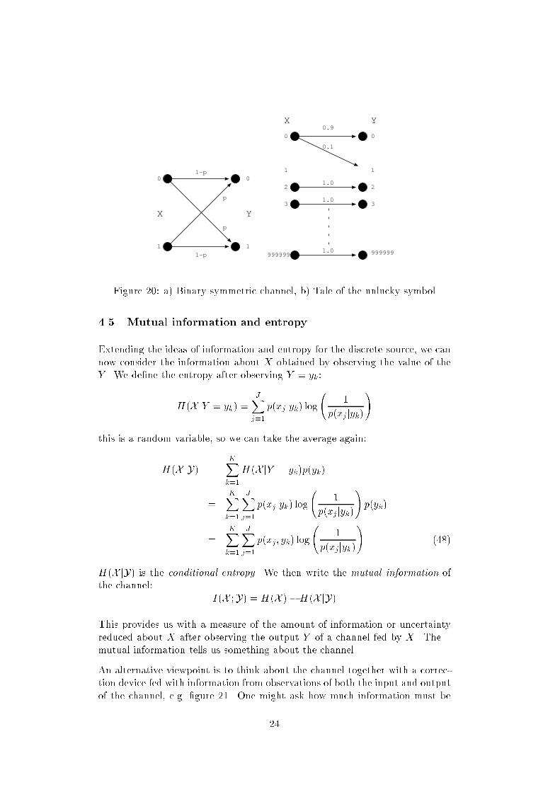
999999999999Figure 20: a) Binary symmetric channel, b) Tale of the unlucky symbol4.5 Mutual information and entropyExtending the ideas of information and entropy for the discrete source, we cannow consider the information about X obtained by observing the value of theY . We dene the entropy after observing Y = yk :H(X jY = yk) = JXj=1 p(xj jyk) log 1p(xj jyk)!this is a random variable, so we can take the average again:H(X jY) = KXk=1H(X jY = yk)p(yk)= KXk=1 JXj=1 p(xjjyk) log 1p(xj jyk)! p(yk)= KXk=1 JXj=1 p(xj; yk) log 1p(xjjyk)! (48)H(X jY) is the conditional entropy. We then write the mutual information ofthe channel: I(X ;Y) = H(X )H(X jY)This provides us with a measure of the amount of information or uncertaintyreduced about X after observing the output Y of a channel fed by X . Themutual information tells us something about the channel.An alternative viewpoint is to think about the channel together with a correc-tion device fed with information from observations of both the input and outputof the channel, e.g. gure 21. One might ask how much information must be24

Sourceencoder Decoder

X Y XCorrection

Observer

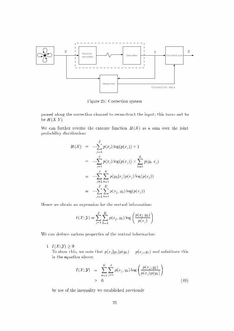
Correction dataFigure 21: Correction systempassed along the correction channel to reconstruct the input; this turns out tobe H(X jY ).We can further rewrite the entropy function H(X ) as a sum over the jointprobability distribution:H(X ) = JXj=1 p(xj) log(p(xj)) 1= JXj=1 p(xj) log(p(xj)) KXk=1 p(ykjxj)= JXj=1 KXk=1 p(ykjxj)p(xj) log(p(xj))= JXj=1 KXk=1 p(xj; yk) log(p(xj))Hence we obtain an expression for the mutual information:I(X ;Y) = JXj=1 KXk=1 p(xj; yk) log p(xjjyk)p(xj) !We can deduce various properties of the mutual information:1. I(X ;Y) 0.To show this, we note that p(xj jyk)p(yk) = p(xj ; yk) and substitute thisin the equation above:I(X ;Y) = KXk=1 JXj=1 p(xj; yk) log p(xj; yk)p(xj)p(yk)! 0 (49)by use of the inequality we established previously.25

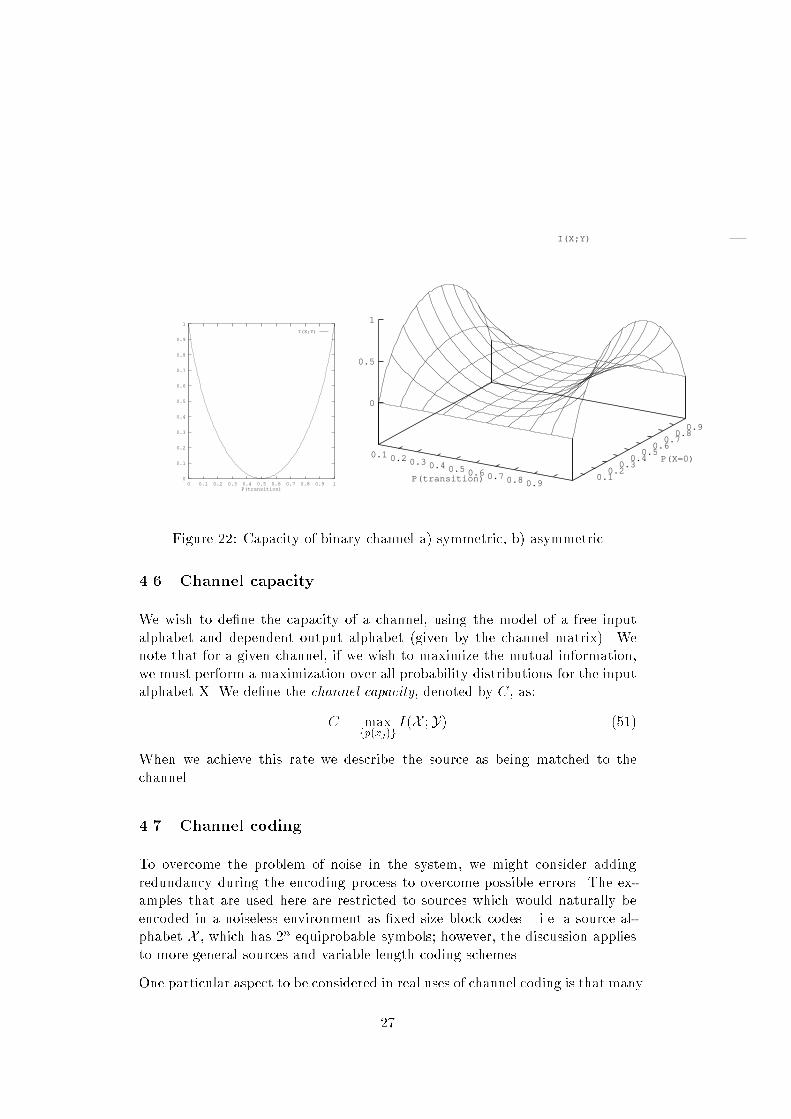
2. I(X ;Y) = 0 if X and Y are statistically independent.If X and Y are independent, p(xj ; yk) = p(xj)p(yk), hence the log termbecomes zero.3. I is symmetric, I(X ;Y) = I(Y ;X ).Using p(xj jyk)p(yk) = p(ykjxj)p(xj), we obtain:I(X ;Y) = JXj=1 KXk=1 p(xj ; yk) log p(xj jyk)p(xj) != JXj=1 KXk=1 p(xj ; yk) logp(ykjxj)p(yk) = I(Y ;X) (50)4. The preceding leads to the obvious symmetric denition for the mutualinformation in terms of the entropy of the output:I(X ;Y) = H(Y)H(YjX )5. We dene the joint entropy of two random variables in the obvious man-ner, based on the joint probability distribution:H(X ;Y) = JXj=1 KXk=1 p(xj ; yk) log(p(xj; yk))The mutual information is the more naturally written:I(X ;Y) = H(X ) +H(Y)H(X ;Y)4.5.1 Binary channelConsider the conditional entropy and mutual information for the binary sym-metric channel. The input source has alphabet X = f0; 1g and associatedprobabilities f1=2; 1=2g and the channel matrix is: 1 p pp 1 p !Then the entropy, conditional entropy and mutual information are given by:H(X ) = 1H(X jY) = p log(p) (1 p) log(1 p)I(X ;Y) = 1 + p log(p) + (1 p) log(1 p)Figure 22a shows the capacity of the channel against transition probability.Note that the capacity of the channel drops to zero when the transition proba-bility is 1/2, and is maximized when the transition probability is 0; or 1 if wereliably transpose the symbols on the wire we also get the maximum amountof information through! Figure 22b shows the eect on mutual information forasymmetric input alphabets. 26

0

0.1

0.2

0.3

0.4

0.5

0.6

0.7

0.8

0.9

1

0 0.1 0.2 0.3 0.4 0.5 0.6 0.7 0.8 0.9 1P(transition)

I(X;Y)

I(X;Y)

0.1 0.2 0.3 0.4 0.5 0.6 0.7 0.8 0.90.1

0.20.3

0.40.5

0.60.7

0.80.9

0

0.5

1

P(transition)

P(X=0)Figure 22: Capacity of binary channel a) symmetric, b) asymmetric4.6 Channel capacityWe wish to dene the capacity of a channel, using the model of a free inputalphabet and dependent output alphabet (given by the channel matrix). Wenote that for a given channel, if we wish to maximize the mutual information,we must perform a maximization over all probability distributions for the inputalphabet X. We dene the channel capacity, denoted by C, as:C = maxfp(xj)g I(X ;Y) (51)When we achieve this rate we describe the source as being matched to thechannel.4.7 Channel codingTo overcome the problem of noise in the system, we might consider addingredundancy during the encoding process to overcome possible errors. The ex-amples that are used here are restricted to sources which would naturally beencoded in a noiseless environment as xed size block codes i.e. a source al-phabet X , which has 2n equiprobable symbols; however, the discussion appliesto more general sources and variable length coding schemes.One particular aspect to be considered in real uses of channel coding is that many27

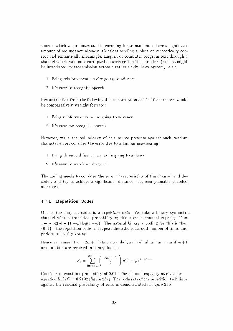
sources which we are interested in encoding for transmissions have a signicantamount of redundancy already. Consider sending a piece of syntactically cor-rect and semantically meaningful English or computer program text through achannel which randomly corrupted on average 1 in 10 characters (such as mightbe introduced by transmission across a rather sickly Telex system). e.g.:1. Bring reinforcements, we're going to advance2. It's easy to recognise speechReconstruction from the following due to corruption of 1 in 10 characters wouldbe comparatively straight forward:1. Brizg reinforce ents, we're going to advance2. It's easy mo recognise speechHowever, while the redundancy of this source protects against such randomcharacter error, consider the error due to a human mis-hearing:1. Bring three and fourpence, we're going to a dance.2. It's easy to wreck a nice peach.The coding needs to consider the error characteristics of the channel and de-coder, and try to achieve a signicant \distance" between plausible encodedmessages.4.7.1 Repetition CodesOne of the simplest codes is a repetition code. We take a binary symmetricchannel with a transition probability p; this gives a channel capacity C =1 + p log(p) + (1 p) log(1 p). The natural binary encoding for this is thenf0; 1g the repetition code will repeat these digits an odd number of times andperform majority voting.Hence we transmit n = 2m+1 bits per symbol, and will obtain an error if m+1or more bits are received in error, that is:Pe = 2m+1Xi=m+1 2m+ 1i ! pi(1 p)2m+1iConsider a transition probability of 0:01. The channel capacity as given byequation 51 is C = 0:9192 (gure 23a). The code rate of the repetition techniqueagainst the residual probability of error is demonstrated in gure 23b.28

0.9

0.91

0.92

0.93

0.94

0.95

0.96

0.97

0.98

0.99

1

1e-08 1e-07 1e-06 1e-05 0.0001 0.001 0.01 0.1

Capacity

P(transition)

I(X;Y)(p)I(X;Y)(0.01)

1e-10

1e-09

1e-08

1e-07

1e-06

1e-05

0.0001

0.001

0.01

0.1

0.01 0.1 1

Residual error rate

Code rate

Repetitiion codeH(0.01)

Figure 23: a) Capacity of binary symmetric channel at low loss rates, b) E-ciency of repetition code for a transition probability of 0:014.8 Channel Coding TheoremWe arrive at Shannon's second theorem, the channel coding theorem:For a channel of capacity C and a source of entropy H ; if H C,then for arbitrarily small , there exists a coding scheme such thatthe source is reproduced with a residual error rate less than .Shannon's proof of this theorem is an existence proof rather than a means toconstruct such codes in the general case. In particular the choice of a goodcode is dictated by the characteristics of the channel noise. In parallel with thenoiseless case, better codes are often achieved by coding multiple input symbols.4.8.1 An ecient codingConsider a rather articial channel which may randomly corrupt one bit in eachblock of seven used to encode symbols in the channel we take the probabil-ity of a bit corruption event is the same as correct reception. We inject Nequiprobable input symbols (clearly N 27 for unique decoding). What is thecapacity of this channel?We have 27 input and output patterns; for a given input xj with binary digitrepresentation b1b2b3b4b5b6b7, we have eight equiprobable (i.e. with 1/8 proba-bility) output symbols (and no others):29

b1b2b3b4b5b6b7b1b2b3b4b5b6b7b1 b2b3b4b5b6b7b1b2 b3b4b5b6b7b1b2b3 b4b5b6b7b1b2b3b4 b5b6b7b1b2b3b4b5 b6b7b1b2b3b4b5b6 b7Then considering the information capacity per symbol:C = max(H(Y)H(Y jX))= 17 0@7Xj Xk p(ykjxj) log 1p(ykjxj)! p(xj)1A= 17 0@7 +Xj 8(18 log 18) 1N1A= 17 7 +N(88 log 18) 1N= 47The capacity of the channel is 4=7 information bits per binary digit of thechannel coding. Can we nd a mechanism to encode 4 information bits in 7channel bits subject to the error property described above?The (7/4) Hamming Code provides a systematic code to perform this a sys-tematic code is one in which the obvious binary encoding of the source symbolsis present in the channel encoded form. For our source which emits at each timeinterval 1 of 16 symbols, we take the binary representation of this and copy itto bits b3, b5, b6 and b7 of the encoded block; the remaining bits are given byb4; b2; b1, and syndromes by s4; s2; s1:b4 = b5 b6 b7 and,s4 = b4 b5 b6 b7b2 = b3 b6 b7 and,s2 = b2 b3 b6 b7b1 = b3 b5 b7 and,s1 = b1 b3 b5 b7On reception if the binary number s4s2s1 = 0 then there is no error, else bs4s2s1is the bit in error.This Hamming code uses 3 bits to correct 7 (= 23 1) error patterns andtransfer 4 useful bits. In general a Hamming code uses m bits to correct 2m 1error patterns and transfer 2m 1 m useful bits. The Hamming codes arecalled perfect as they use m bits to correct 2m 1 errors.30

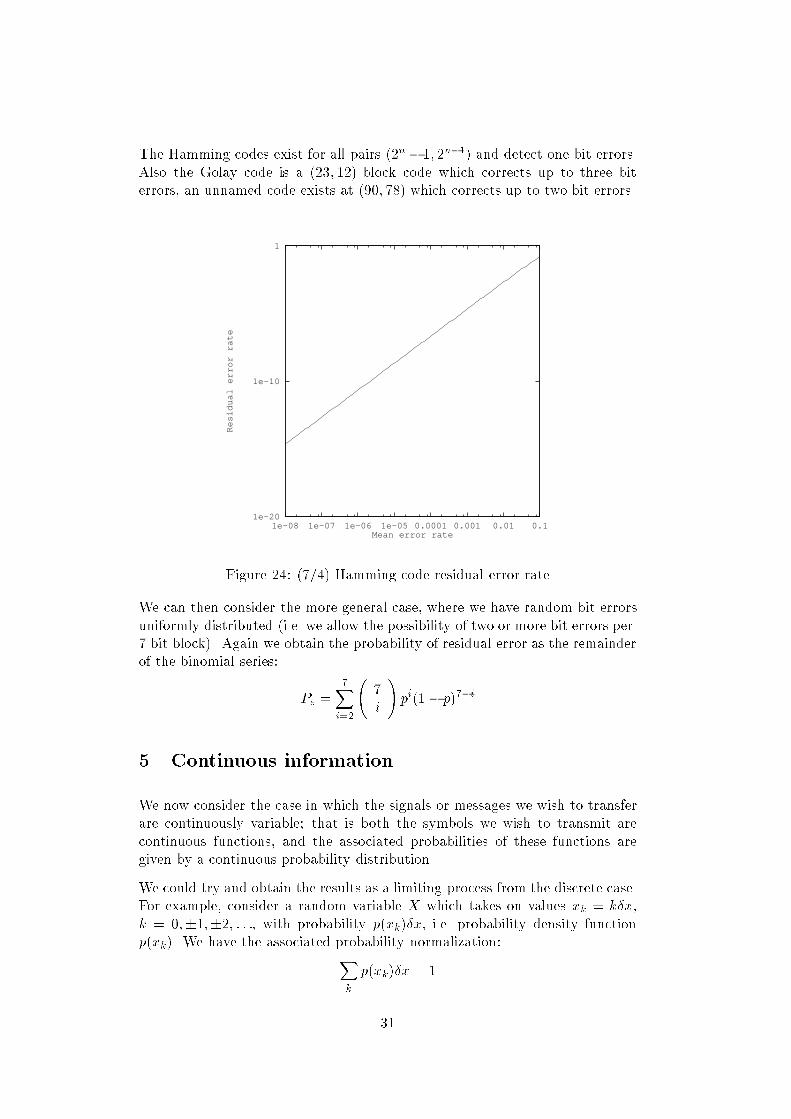
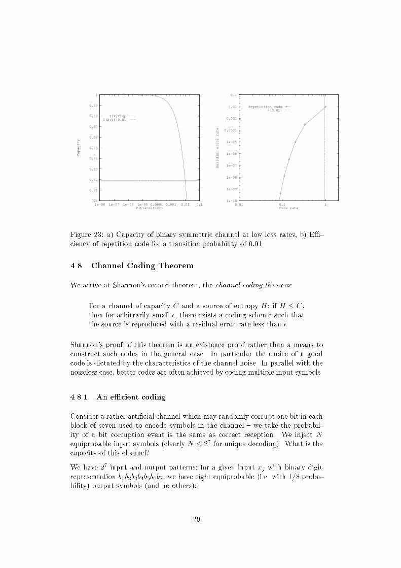
The Hamming codes exist for all pairs (2n 1; 2n1) and detect one bit errors.Also the Golay code is a (23; 12) block code which corrects up to three biterrors, an unnamed code exists at (90; 78) which corrects up to two bit errors.1e-20

1e-10

1

1e-08 1e-07 1e-06 1e-05 0.0001 0.001 0.01 0.1

Residual error rate

Mean error rateFigure 24: (7/4) Hamming code residual error rateWe can then consider the more general case, where we have random bit errorsuniformly distributed (i.e. we allow the possibility of two or more bit errors per7 bit block). Again we obtain the probability of residual error as the remainderof the binomial series: Pe = 7Xi=2 7i ! pi(1 p)7i5 Continuous informationWe now consider the case in which the signals or messages we wish to transferare continuously variable; that is both the symbols we wish to transmit arecontinuous functions, and the associated probabilities of these functions aregiven by a continuous probability distribution.We could try and obtain the results as a limiting process from the discrete case.For example, consider a random variable X which takes on values xk = kx,k = 0;1;2; : : :, with probability p(xk)x, i.e. probability density functionp(xk). We have the associated probability normalization:Xk p(xk)x = 131

Using our formula for discrete entropy and taking the limit:H(X ) = limx!0Xk p(xk)x log2 1p(xk)x= limx!0"Xk p(xk) log2 1p(xk) x log2(x)Xk p(x)x#= Z 11 p(x) log2 1p(x)dx limx!0 log2(x) Z 11 p(x)dx= h(X ) limx!0 log2(x) (52)This is rather worrying as the latter limit does not exist. However, as we areoften interested in the dierences between entropies (i.e. in the considerationof mutual entropy or capacity), we dene the problem away by using the rstterm only as a measure of dierential entropy:h(X ) = Z 11 p(x) log2 1p(x)dx (53)We can extend this to a continuous random vector of dimension n concealingthe n-fold integral behind vector notation and bold type:h(X) = Z 11 p(x) log2 1p(x)dx (54)We can then also dene the joint and conditional entropies for continuous dis-tributions: h(X;Y) = Z Z p(x;y) log2 1p(x;y)dxdyh(XjY) = Z Z p(x;y) log2 p(y)p(x;y)dxdyh(YjX) = Z Z p(x;y) log2 p(x)p(x;y)dxdywith: p(x) = Z p(x;y)dyp(y) = Z p(x;y)dxFinally, mutual information of continuous random variables X and Y is denedusing the double integral:i(X ; Y ) = Z Z p(x; y) logp(xjy)p(x) dxdywith the capacity of the channel given by maximizing this mutual informationover all possible input distributions for X .32

5.1 PropertiesWe obtain various properties analagous to the discrete case. In the followingwe drop the bold type, but each distribution, variable etc should be taken tobe of n dimensions.1. Entropy is maximized with equiprobable \symbols". If x is limited tosome volume v (i.e. is only non-zero within the volume) then h(x) is max-imized when p(x) = 1=v.2. h(x; y) h(x) + h(y)3. What is the maximum dierential entropy for specied variance wechoose this as the variance is a measure of average power. Hence a re-statement of the problem is to nd the maximum dierential entropy fora specied mean power.Consider the 1-dimensional random variable X , with the constraints:Z p(x)dx = 1Z (x )2p(x)dx = 2where: = Z xp(x)dx (55)This optimization problem is solved using Lagrange multipliers and max-imizing: Z p(x) log p(x) + 1p(x)(x )2 + 2p(x)dxwhich is obtained by solving:1 log p(x) + 1(x )2 + 2 = 0so that with due regard for the constraints on the system:p(x) = 1p2e(x)2=22hence: h(X) = 12 log(2e2) (56)We observe that: i) for any random variable Y with variance , h(Y ) h(X), ii) the dierential entropy is dependent only on the variance andis independent of the mean, hence iii) the greater the power, the greaterthe dierential entropy.This extends to multiple dimensions in the obvious manner.33

5.2 EnsemblesIn the case of continuous signals and channels we are interested in functions (ofsay time), chosen from a set of possible functions, as input to our channel, withsome perturbed version of the functions being detected at the output. Thesefunctions then take the place of the input and output alphabets of the discretecase.We must also then include the probability of a given function being injectedinto the channel which brings us to the idea of ensembles this general area ofwork is known as measure theory.For example, consider the ensembles:1. f(t) = sin(t+ )Each value of denes a dierent function, and together with a probabilitydistribution, say p (), we have an ensemble. Note that here may bediscrete or continuous consider phase shift keying.2. Consider a set of random variables fai: i = 0;1;2; : : :g where eachai takes on a random value according to a Gaussian distribution withstandard deviation pN ; then:f(faig; t) =Xi aisinc(2Wt i)is the \white noise" ensemble, band- limited to W Hertz and with averagepower N .3. More generally, we have for random variables fxig the ensemble of band-limited functions: f(fxig; t) =Xi xisinc(2Wt i)where of course we remember from the sampling theorem that:xi = f i2W If we also consider functions limited to time interval T , then we ob-tain only 2TW non-zero coecients and we can consider the ensembleto be represented by an n-dimensional (n = 2TW )probability distributionp(x1; x2; : : : ; xn).4. More specically, if we consider the ensemble of limited power (by P ),band- limited (to W ) and time- limited signals (non-zero only in interval(0; T )), we nd that the ensemble is represented by an n-dimensionalprobability distribution which is zero outside the n-sphere radius r =p2WP . 34

By considering the latter types of ensembles, we can t them into the nitedimensional continuous dierential entropy denitions given in section 5.5.3 Channel CapacityWe consider channels in which noise is injected independently of the signal; theparticular noise source of interest is the so- called additive white Gaussian noise.Further we restrict considerations to the nal class of ensemble.We have a signal with average power P , time- limited to T and bandwidthlimited to W .We then consider the n = 2WT samples (Xk and Yk) that can be used tocharacterise both the input and output signals. Then the relationship betweenthe input and output is given by:Yk = Xk +Nk , k = 1; 2; : : :nwhere Nk is from the band- limited Gaussian distribution with zero mean andvariance: 2 = N0Wwhere N0 is the power spectral density.As N is independent of X we obtain the conditional entropy as being solelydependent on the noise source, and from equation 56 nd its value:h(Y jX) = h(N) = 12 log 2eN0WHence: i(X ; Y ) = h(Y ) h(N)The capacity of the channel is then obtained by maximizing this over all inputdistributions this is achieved by maximizing with respect to the distributionof X subject to the average power limitation:E[X2k ] = PAs we have seen this is achieved when we have a Gaussian distribution, hencewe nd both X and Y must have Gaussian distributions. In particular X hasvariance P and Y has variance P +N0W .We can then evaluate the channel capacity, as:h(Y ) = 12 log 2e(P +N0W )h(N) = 12 log 2e(N0W )C = 12 log1 + PN0W (57)35

This capacity is in bits per channel symbol, so we can obtain a rate per second,by multiplication by n=T , i.e. from n = 2WT , multiplication by 2W :C = W log 2 1 + PN0W bit/sSo Shannon's third theorem, the noisy-channel coding theorem:The capacity of a channel bandlimited to W Hertz, perturbed byadditive white Gaussian noise of power spectral density N0 and band-limited to W is given by:C = W log 2 1 + PN0W bit/s (58)where P is the average transmitted power.5.3.1 NotesThe second term within the log in equation 58 is the signal to noise ratio (SNR).1. Observe that the capacity increases monotonically and without boundas the SNR increases.2. Similarly the capacity increases monotonically as the bandwidth increasesbut to a limit. Using Taylor's expansion for ln:ln(1 + ) = 22 + 33 44 + we obtain: C ! PN0 log2 e3. This is often rewritten in terms of energy per bit, Eb, which is dened byP = EbC. The limiting value is then:EbN0 ! loge 2 = 0:693This is called the Shannon Limit.4. The capacity of the channel is achieved when the source \looks like noise".This is the basis for spread spectrum techniques of modulation and inparticular Code Division Multiple Access (CDMA).36

1. Foundations: Probability, Uncertainty, and Information2. Entropies Defined, and Why they are Measures of Information3. Source Coding Theorem; Prefix, Variable-, and Fixed-Length Codes4. Channel Types, Properties, Noise, and Channel Capacity5. Continuous Information; Density; Noisy Channel Coding Theorem6. Fourier Series, Convergence, Orthogonal Representation

7. Useful Fourier Theorems; Transform Pairs; Sampling; Aliasing

8. Discrete Fourier Transform. Fast Fourier Transform Algorithms9. The Quantized Degrees-of-Freedom in a Continuous Signal10. Gabor-Heisenberg-Weyl Uncertainty Relation. Optimal “Logons”11. Kolmogorov Complexity and Minimal Description Length.

Jean Baptiste Joseph Fourier (1768 - 1830)

37

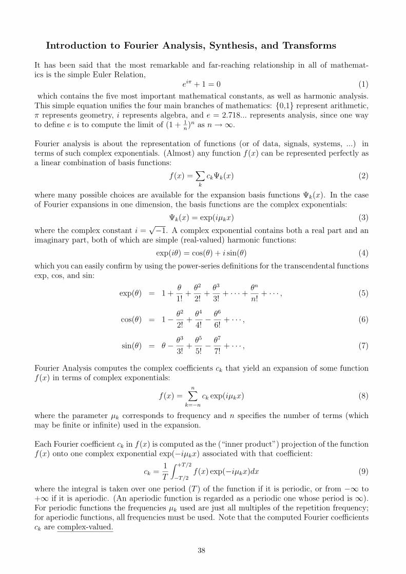
Introduction to Fourier Analysis, Synthesis, and Transforms

It has been said that the most remarkable and far-reaching relationship in all of mathemat-ics is the simple Euler Relation,

eiπ + 1 = 0 (1)

which contains the five most important mathematical constants, as well as harmonic analysis.This simple equation unifies the four main branches of mathematics: 0,1 represent arithmetic,π represents geometry, i represents algebra, and e = 2.718... represents analysis, since one wayto define e is to compute the limit of (1 + 1

n)n as n → ∞.

Fourier analysis is about the representation of functions (or of data, signals, systems, ...) interms of such complex exponentials. (Almost) any function f(x) can be represented perfectly asa linear combination of basis functions:

f(x) =∑

k

ckΨk(x) (2)

where many possible choices are available for the expansion basis functions Ψk(x). In the caseof Fourier expansions in one dimension, the basis functions are the complex exponentials:

Ψk(x) = exp(iµkx) (3)

where the complex constant i =√−1. A complex exponential contains both a real part and an

imaginary part, both of which are simple (real-valued) harmonic functions:

exp(iθ) = cos(θ) + i sin(θ) (4)

which you can easily confirm by using the power-series definitions for the transcendental functionsexp, cos, and sin:

exp(θ) = 1 +θ

1!+

θ2

2!+

θ3

3!+ · · · + θn

n!+ · · · , (5)

cos(θ) = 1 − θ2

2!+

θ4

4!− θ6

6!+ · · · , (6)

sin(θ) = θ − θ3

3!+

θ5

5!− θ7

7!+ · · · , (7)

Fourier Analysis computes the complex coefficients ck that yield an expansion of some functionf(x) in terms of complex exponentials:

f(x) =n

∑

k=−n

ck exp(iµkx) (8)

where the parameter µk corresponds to frequency and n specifies the number of terms (whichmay be finite or infinite) used in the expansion.

Each Fourier coefficient ck in f(x) is computed as the (“inner product”) projection of the functionf(x) onto one complex exponential exp(−iµkx) associated with that coefficient:

ck =1

T

∫ +T/2

−T/2f(x) exp(−iµkx)dx (9)

where the integral is taken over one period (T ) of the function if it is periodic, or from −∞ to+∞ if it is aperiodic. (An aperiodic function is regarded as a periodic one whose period is ∞).For periodic functions the frequencies µk used are just all multiples of the repetition frequency;for aperiodic functions, all frequencies must be used. Note that the computed Fourier coefficientsck are complex-valued.

38

1 Fourier Series and TransformsConsider real valued periodic functions f(x), i.e. for some a and 8x, f(x+a) =f(x). Without loss of generality we take a = 2.We observe the orthogonality properties of sin(mx) and cos(nx) for integers mand n: Z 20 cos(nx) cos(mx)dx = ( 2 if m = n = 0mn otherwiseZ 20 sin(nx) sin(mx)dx = ( 0 if m = n = 0mn otherwiseZ 20 sin(nx) cos(mx)dx = 0 8m;n (1)We use the Kronecker function to mean:mn = ( 1 m = n0 otherwiseThen the Fourier Series for f(x) is:a02 + 1Xn=1 (an cos(nx) + bn sin(nx)) (2)where the Fourier Coecients are:an = 1Z 20 f(x) cos(nx)dx n 0 (3)bn = 1 Z 20 f(x) sin(nx)dx n 1 (4)We hope that the Fourier Series provides an expansion of the function f(x) interms of cosine and sine terms.1.1 Approximation by least squaresLet S 0N (x) be any sum of sine and cosine terms:S0N (x) = a002 + N1Xn=1(a0n cos(nx) + b0n sin(nx)) (5)and SN (x), the truncated Fourier Series for a function f(x):SN (x) = a02 + N1Xn=1(an cos(nx) + bn sin(nx))39

where an and bn are the Fourier coecients. Consider the integral giving thediscrepancy between f(x) and S 0n(x) (assuming f(x) is well behaved enough forthe integral to exist): Z 20 f(x) S 0n(x)2 dxwhich simplies to:Z 20 ff(x)g2 dx 2a20 N1Xn=1(a2n + b2n)+ 2(a00 a0)2 + N1Xn=1 n(a0n an)2 + (b0n bn)2o (6)Note that the terms involving a0 and b0 are all 0 and vanish when a0n = anand b0n = bn. The Fourier Series is the best approximation, in terms of meansquared error, to f that can be achieved using these circular functions.1.2 Requirements on functionsThe Fourier Series and Fourier coecients are dened as above. However wemay encounter some problems:1. integrals in equations 3, 4 fail to exist. e.g.:f(x) = 1xor f(x) = ( 1 x rational0 x irrational2. although an, bn exist, the series does not converge,3. even though the series converges, the result is not f(x)f(x) = ( +1 0 x < 1 x < 2then: an = 0; bn = 2 Z 0 sin(nx)dx = ( 4n n odd0 n evenso: f(x) ?= 4 sin(x) + sin(3x)3 + sin(5x)5 + but series gives f(n) ?= 0. 40

-1.5

-1

-0.5

0

0.5

1

1.5

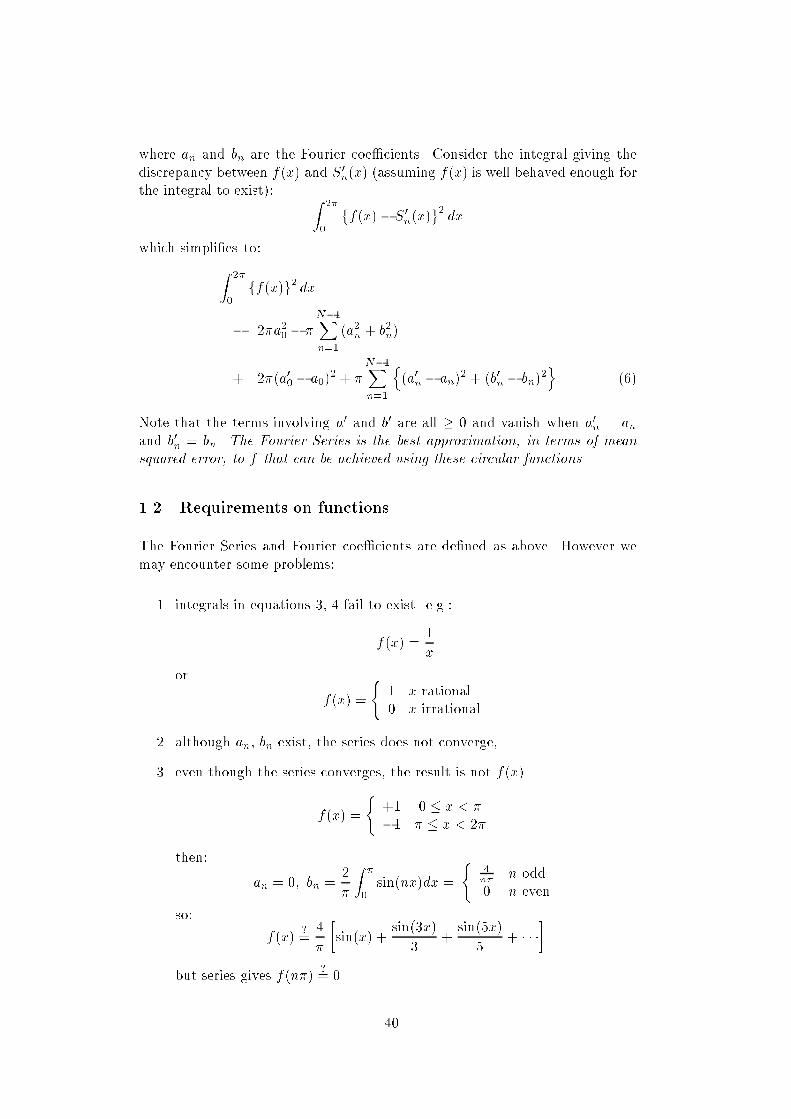
-1 0 1 2 3 4 5 6 7

fseries( 1,x)fseries( 7,x)fseries(63,x)

rect(x)

Figure 1: Approximations to rectangular pulse-1.5

-1

-0.5

0

0.5

1

1.5

-0.2 -0.15 -0.1 -0.05 0 0.05 0.1 0.15 0.2

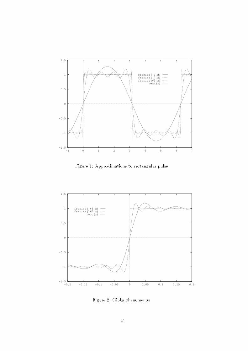
fseries( 63,x)fseries(163,x)

rect(x)

Figure 2: Gibbs phenomenon41

However, in real life examples encountered in signal processing things are sim-pler as:1. If f(x) is bounded in (0; 2) and piecewise continuous, the Fourier seriesconverges to ff(x) + f(x+)g =2 at interior points and ff(0+) + f(2)g =2at 0 and 2. 12. If f(x) is also continuous on (0; 2), the sum of the Fourier Series is equalto f(x) at all points.3. an and bn tend to zero at least as fast as 1=n.1.3 Complex formRewrite using einx in the obvious way from the formulae for sin and cos:f(x)= a02 + 1Xn=1 (an cos(nx) + bn sin(nx))= a02 + 1Xn=1 an (einx + einx)2 + bn (einx einx)2i != 1X1 cneinx (7)with: c0 = a0=2n > 0 cn = (an ibn)=2cn = (an + ibn)=2observe: cn = cn (8)where c denotes the complex conjugate, and:cn = 12 Z 20 f(x)einxdx (9)1.4 Approximation by interpolationConsider the value of a periodic function f(x) at N discrete equally spacedvalues of x: xr = r ( = 2N , r = 0; 1; : : : ; N 1)try to nd coecients cn such that:f(r) = N1Xn=0 cneirn (10)1A notation for limits is introduced here f(x) = lim!0 f(x) and f(x+) = lim!0 f(x+). 42

Multiply by eirm and sum with respect to r:N1Xr=0 f(r)eirm = N1Xr=0 N1Xn=0 cneir(nm)but by the sum of a geometric series and blatant assertion:N1Xr=0 eir(nm) = 8>>><>>>: 1 eiN(nm)1 ei(nm) = 0 n 6= mN n = mso: cm = 1N N1Xr=0 f(r)eirm (11)Exercise for the reader: show inserting equation 11 into equation 10 satisesthe original equations.-5

-4

-3

-2

-1

0

1

2

3

4

0 2 4 6 8 10 12

saw(x)’trig.pts.8’’trig.pts.64’

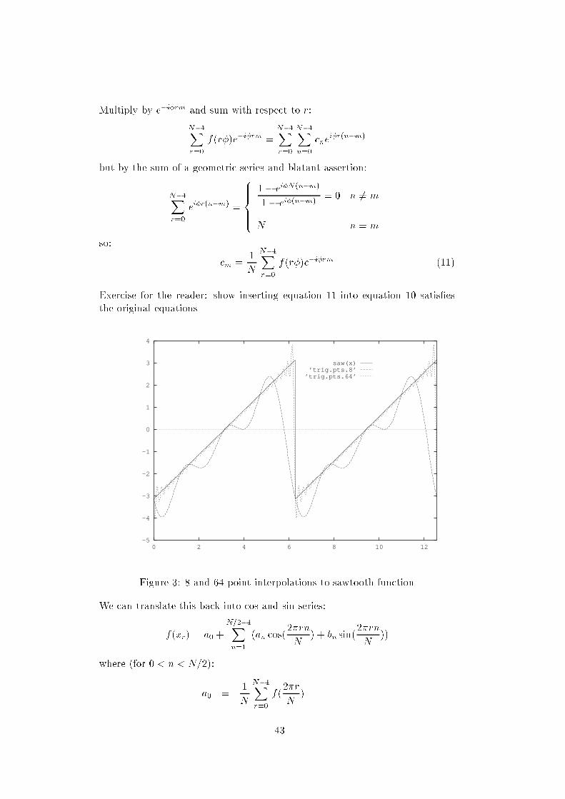
Figure 3: 8 and 64 point interpolations to sawtooth functionWe can translate this back into cos and sin series:f(xr) = a0 + N=21Xn=1 (an cos(2rnN ) + bn sin(2rnN ))where (for 0 < n < N=2):a0 = 1N N1Xr=0 f(2rN )43

an = 2N N1Xr=0 f(2rN ) cos(2rnN )bn = 2N N1Xr=0 f(2rN ) sin(2rnN ) (12)As we increase N we can make the interpolation function agree with f(x) atmore and more points. Taking an as an example, as n ! 1 (for well behavedf(x)): an = 1 N1Xr=0 f(2rN ) cos(2rnN )2N ! 1 Z 20 f(x) cos(nx)dx (13)1.5 Cosine and Sine SeriesObserve that if f(x) is symmetric, that is f(x) = f(x) then:a0 = 2 Z 0f(x)dxan = 2 Z 0f(x) cos(nx)dxbn = 0hence the Fourier series is simply:a02 +Xn>0 an cos(nx)On the other hand if f(x) = f(x): then we get the corresponding sine series:Xn>0 bn sin(nx)with: bn = 2 Z 0f(x) sin(nx)dxExample, take f(x) = 1 for 0 < x < . We can extend this to be periodicwith period 2 either symmetrically, when we obtain the cosine series (whichis simply a0 = 2 as expected), or with antisymmetry (square wave) when thesine series gives us:1 = 4 sin(x) + sin(3x)3 + sin(5x)5 + (for 0 < x < )Another example, take f(x) = x( x) for 0 < x < . The cosine series is:f(x) = 26 cos(2x) cos(4x)22 cos(6x)32 44

hence as f(x)! 0 as x! 0:26 = 1 + 122 + 132 + the corresponding sine series is:x( x) = 8 sin(x) + sin(3x)33 + sin(5x)53 + and at x = =2: 3 = 32 1 133 + 153 Observe that one series converges faster than the other, when the values of thebasis functions match the values of the function at the periodic boundaries.1.6 Fourier transformStarting from the complex series in equation 9, make a change of scale considera periodic function g(x) with period 2X ; dene f(x) = g(xX=), which hasperiod 2. cn = 12 Z f(x)einxdx= 12 X Z XX g(y)einy=Xdyc(k) = 12 Z XX g(y)eikydy (14)where k = n=X, and c(k) = Xcn=. Hence:f(x) = Xn cneinxg(y) = Xk c(k)eiky X= Xk c(k)eikyk (15)writing k for the step =X . Allowing X ! 1, then we hope:Xk c(k)eikyk! Z 11G(k)eikydkHence we obtain the Fourier Transform pair:g(x) = 12 Z 11G(k)eikxdk (16)G(k) = Z 11 g(x)eikxdx (17)45

Equation 16 expresses a function as a spectrum of frequency components. Takentogether (with due consideration for free variables) we obtain:f(x) = 12 Z 11 Z 11 f(y)eik(xy)dkdy (18)Fourier's Integral Theorem is a statement of when this formula holds; if f(x) isof bounded variation, and jf(x)j is integrable from 1 to1, then equation 18holds (well more generally the double integral gives (f(x+) + f(x))=2).1.7 FT PropertiesWriting g(x)*) G(k) to signify the transform pair, we have the following prop-erties:1. Symmetry and reality if g(x) real then G(k) = G(k) if g(x) real and even:G(k) = 2 Z 10 f(x) cos(kx)dx if g(x) real and oddG(k) = 2i Z 10 f(x) sin(kx)dxThe last two are analogues of the cosine and sine series cosine and sinetransforms.2. Linearity; for constants a and b, if g1(x) *) G1(k) and g2(x) *) G2(k)then ag1(x) + bg2(x)*) aG1(k) + bG2(k)3. Space/time shifting g(x a) *) eikaG(k)4. Frequency shifting g(x)eix *) G(k )5. Dierentiation once g0(x)*) ikG(k)6. . . . and n times, g(n)(x)*) (ik)nG(k)1.8 ConvolutionsSuppose f(x) *) F (k), g(x) *) G(k); what function h(x) has a transformH(k) = F (k)G(k)? Inserting into the inverse transform:h(x) = 12 Z F (k)G(k)eikxdk= 12 Z Z Z f(y)g(z)eik(xyz)dkdydz= 12 Z Z Z f(y)g( y)eik(x)dkdyd46

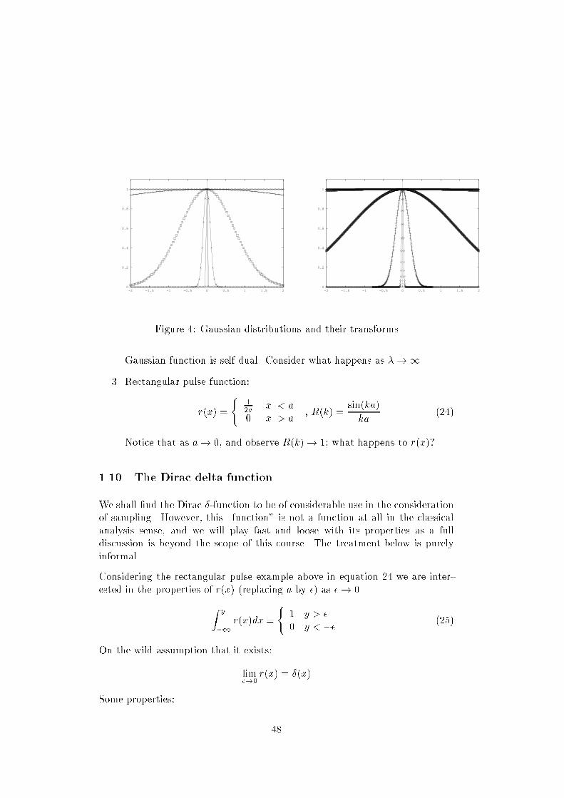
From equation 18, we then obtain the convolution of f and g:h(x) = Z 11 f(y)g(x y)dy (19)= f(x) ? g(x) (20)or: Z 11 f(y)g(x y)dy *) F (k)G(k)Similarly: f(y)g(y)*) Z 11 F ()G(k )dAs a special case convolve the real functions f(x) and f(x), then:F (k) = F (k)H(k) = F (k)F (k)= jF (k)j2 (21)f(x) = Z 11 f(y)f(y + x)dy (22)The function f in Equation 22 is the autocorrelation function (of f), whilejF (k)j2 in equation 21 is the spectral density. Observe Parseval's theorem:(0) = Z 11[f(y)]2dy = 12 Z 11 jF (k)j2dk1.9 Some FT pairsSome example Transform pairs:1. Simple example:f(x) = ( eax x > 00 x < 0 , F (k) = 1a+ ikIf we make the function symmetric about 0:f(x) = eajxj , F (k) = 2aa2 + k22. Gaussian example (see gure 4):f(x) = e2x2F (k) = Z e2x2ikxdx= e k242 Z e(x+ ik2)2dx= e k242 Z 1+ ik21+ ik2 eu2du= p e k242 (23)47

0

0.2

0.4

0.6

0.8

1

-2 -1.5 -1 -0.5 0 0.5 1 1.5 20

0.2

0.4

0.6

0.8

1

-2 -1.5 -1 -0.5 0 0.5 1 1.5 2Figure 4: Gaussian distributions and their transformsGaussian function is self dual. Consider what happens as !1.3. Rectangular pulse function:r(x) = ( 12a jxj < a0 jxj > a , R(k) = sin(ka)ka (24)Notice that as a! 0, and observe R(k)! 1; what happens to r(x)?1.10 The Dirac delta functionWe shall nd the Dirac -function to be of considerable use in the considerationof sampling. However, this \function" is not a function at all in the classicalanalysis sense, and we will play fast and loose with its properties as a fulldiscussion is beyond the scope of this course. The treatment below is purelyinformal.Considering the rectangular pulse example above in equation 24 we are inter-ested in the properties of r(x) (replacing a by ) as ! 0.Z y1 r(x)dx = ( 1 y > 0 y < (25)On the wild assumption that it exists:lim!0 r(x) = (x)Some properties: 48

1. conceptually (x) = ( `1' x = 00 x 6= 02. taking the limit of equation 25:Z y1 (x)dx = ( 1 y > 00 y < 03. assuming f(x) is continuous in the interval (c ; c + ) and using thedisplaced pulse function r(x c); by the intermediate value theorem forsome in the interval (c ; c+ ):Z 11 f(x)r(x c)dx = f()Hence with usual disregard for rigorousness, taking the limit:Z 11 f(x)(c x)dx = f(c)Observe this is a convolution . . .4. further note g(x)(x c) = g(c)(x c).In some ways the -function and its friends can be considered as analogous toextending the rationals to the reals; they both enable sequences to have limits.We dene the ideal sampling function of interval X as:X(x) =Xn (x nX)we can Fourier transform this (exercise for the reader) and obtain:X(k) = 1X Xm (kX 2m)with X *) X .1.11 Sampling TheoremOur complex and cosine/sine series gave us a discrete set of Fourier coecientsfor a periodic function; or looking at it another way for a function which isnon-zero in a nite range, we can dene a periodic extension of that function.The symmetric nature of the Fourier transform would suggest that somethinginteresting might happen if the Fourier transform function is also non-zero onlyin a nite range. 49

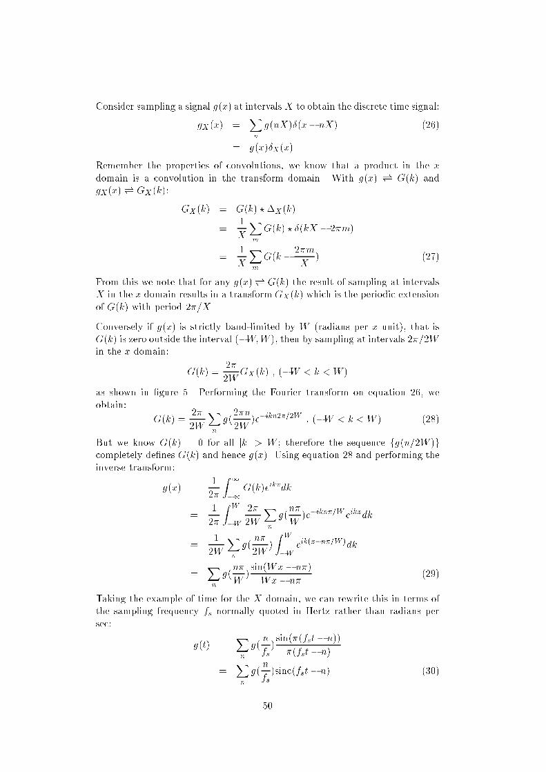
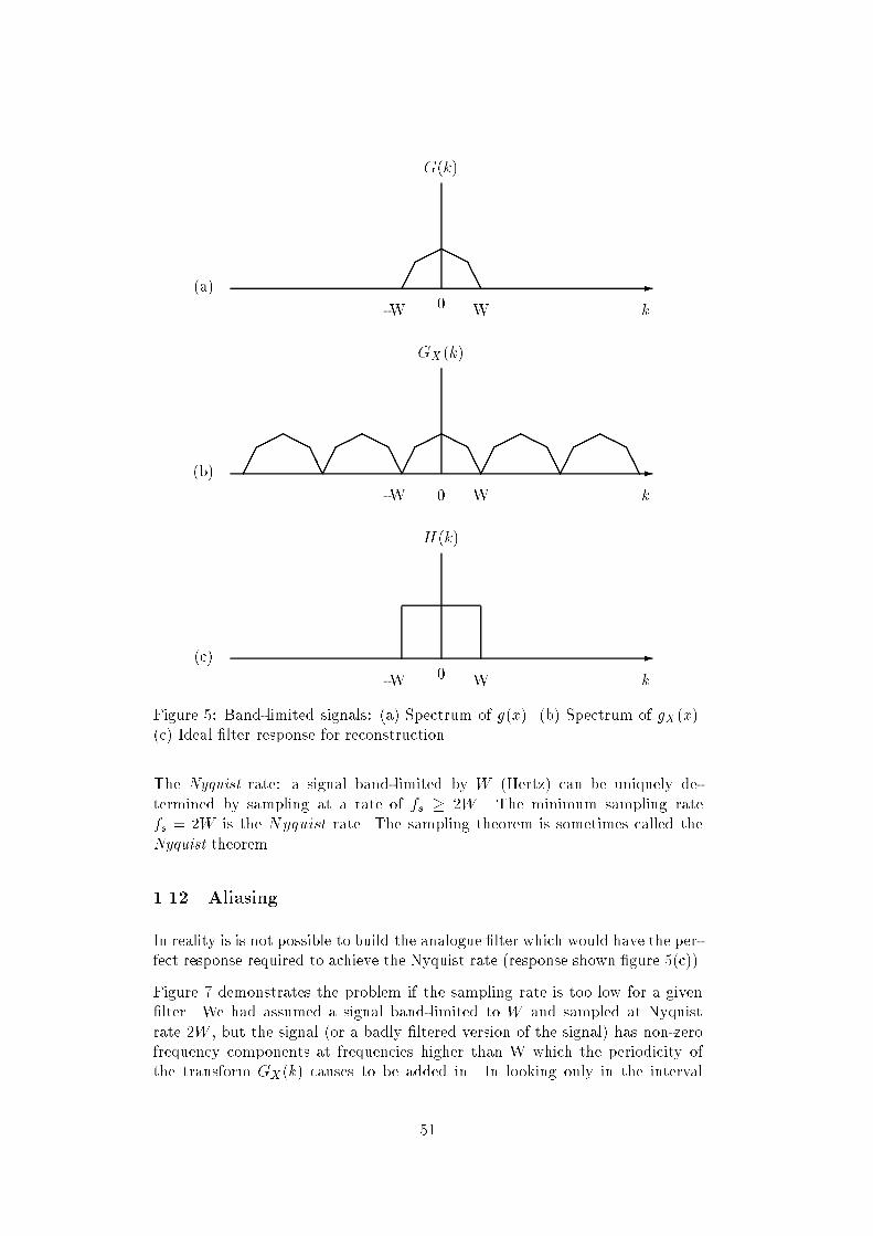
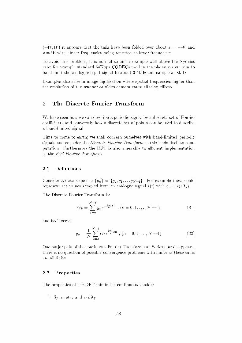
Consider sampling a signal g(x) at intervals X to obtain the discrete time signal:gX(x) = Xn g(nX)(x nX) (26)= g(x)X(x)Remember the properties of convolutions, we know that a product in the xdomain is a convolution in the transform domain. With g(x) *) G(k) andgX(x)*) GX(k): GX(k) = G(k) ?X(k)= 1X Xm G(k) ? (kX 2m)= 1X Xm G(k 2mX ) (27)From this we note that for any g(x)*) G(k) the result of sampling at intervalsX in the x domain results in a transform GX(k) which is the periodic extensionof G(k) with period 2=X .Conversely if g(x) is strictly band-limited by W (radians per x unit), that isG(k) is zero outside the interval (W;W ), then by sampling at intervals 2=2Win the x domain: G(k) = 22WGX(k) , (W < k < W )as shown in gure 5. Performing the Fourier transform on equation 26, weobtain: G(k) = 22W Xn g(2n2W )eikn2=2W , (W < k < W ) (28)But we know G(k) = 0 for all jkj > W ; therefore the sequence fg(n=2W )gcompletely denes G(k) and hence g(x). Using equation 28 and performing theinverse transform:g(x) = 12 Z 11 G(k)eikxdk= 12 Z WW 22W Xn g(nW )eikn=W eikxdk= 12W Xn g( n2W ) Z WW eik(xn=W )dk= Xn g(nW )sin(Wx n)Wx n (29)Taking the example of time for the X domain, we can rewrite this in terms ofthe sampling frequency fs normally quoted in Hertz rather than radians persec: g(t) = Xn g( nfs )sin((fst n))(fst n)= Xn g( nfs )sinc(fst n) (30)50

HHAA k0-W W -HHAAHHAAHHAAHHAAHHAA--

(c) kGX(k)G(k)

-W 0 Wk0-W WH(k)

(a)(b)

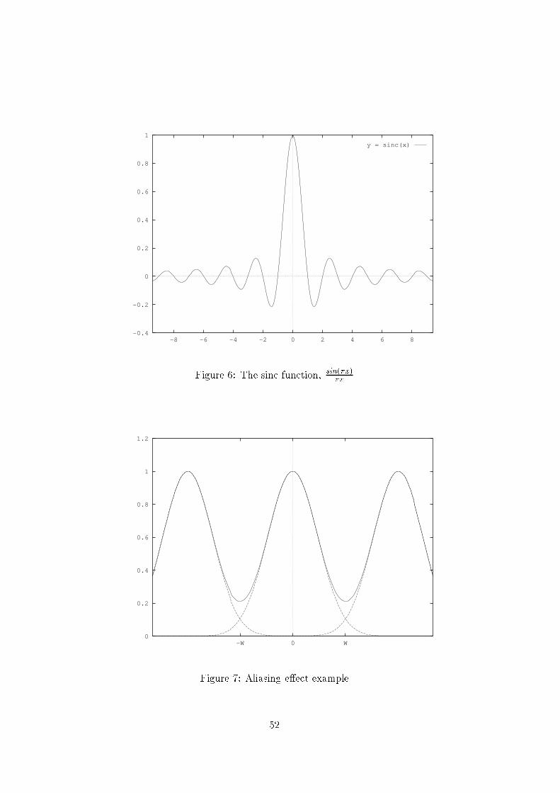
Figure 5: Band-limited signals: (a) Spectrum of g(x). (b) Spectrum of gX(x).(c) Ideal lter response for reconstructionThe Nyquist rate: a signal band-limited by W (Hertz) can be uniquely de-termined by sampling at a rate of fs 2W . The minimum sampling ratefs = 2W is the Nyquist rate. The sampling theorem is sometimes called theNyquist theorem.1.12 AliasingIn reality is is not possible to build the analogue lter which would have the per-fect response required to achieve the Nyquist rate (response shown gure 5(c)).Figure 7 demonstrates the problem if the sampling rate is too low for a givenlter. We had assumed a signal band-limited to W and sampled at Nyquistrate 2W , but the signal (or a badly ltered version of the signal) has non-zerofrequency components at frequencies higher than W which the periodicity ofthe transform GX(k) causes to be added in. In looking only in the interval51

-0.4

-0.2

0

0.2

0.4

0.6

0.8

1

-8 -6 -4 -2 0 2 4 6 8

y = sinc(x)

Figure 6: The sinc function, sin(x)x0

0.2

0.4

0.6

0.8

1

1.2

0-W WFigure 7: Aliasing eect example52

(W;W ) it appears that the tails have been folded over about x = W andx = W with higher frequencies being re ected as lower frequencies.To avoid this problem, it is normal to aim to sample well above the Nyquistrate; for example standard 64Kbps CODECs used in the phone system aim toband-limit the analogue input signal to about 3.4kHz and sample at 8kHz.Examples also arise in image digitization where spatial frequencies higher thanthe resolution of the scanner or video camera cause aliasing eects.2 The Discrete Fourier TransformWe have seen how we can describe a periodic signal by a discrete set of Fouriercoecients and conversely how a discrete set of points can be used to describea band-limited signal.Time to come to earth; we shall concern ourselves with band-limited periodicsignals and consider the Discrete Fourier Transform as this lends itself to com-putation. Furthermore the DFT is also amenable to ecient implementationas the Fast Fourier Transform.2.1 DenitionsConsider a data sequence fgng = fg0; g1; : : :gN1g. For example these couldrepresent the values sampled from an analogue signal s(t) with gn = s(nTs).The Discrete Fourier Transform is:Gk = N1Xn=0 gne 2iN kn , (k = 0; 1; : : : ; N 1) (31)and its inverse: gn = 1N N1Xk=0 Gke 2iN kn , (n = 0; 1; : : : ; N 1) (32)One major pain of the continuous Fourier Transform and Series now disappears,there is no question of possible convergence problems with limits as these sumsare all nite.2.2 PropertiesThe properties of the DFT mimic the continuous version:1. Symmetry and reality 53

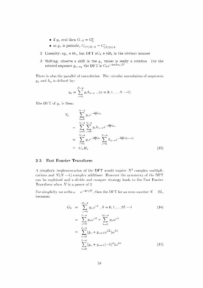
if gn real then Gk = Gk as gn is periodic, G(N=2)k = G(N=2)+k2. Linearity; agn + bhn has DFT aGk + bHk in the obvious manner.3. Shifting; observe a shift in the gn values is really a rotation. For therotated sequence gnn0 the DFT is Gke2ikn0=N .There is also the parallel of convolution. The circular convolution of sequencesgn and hn is dened by:yn = N1Xr=0 grhnr , (n = 0; 1; : : :N 1)The DFT of yn is then:Yk = N1Xn=0 yne 2iN kn= N1Xn=0 N1Xr=0 grhnre 2iN kn= N1Xr=0 gre 2iN kr N1Xr=0 hnre 2iN k(nr)= GkHk (33)2.3 Fast Fourier TransformA simplistic implementation of the DFT would require N2 complex multipli-cations and N(N 1) complex additions. However the symmetry of the DFTcan be exploited and a divide and conquer strategy leads to the Fast FourierTransform when N is a power of 2.For simplicity we write ! = e2i=N , then the DFT for an even number N = 2L,becomes: Gk = 2L1Xn=0 gn!nk , k = 0; 1; : : :2L 1 (34)= L1Xn=0 gn!nk + 2L1Xn=L gn!nk= L1Xn=0(gn + gn+L!kL)!kn= L1Xn=0(gn + gn+L(1)k)!kn (35)54

---------------

----------------

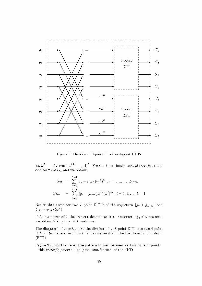
AAAAAAAAAAAAAAUAAAAAAAAAAAAAAUAAAAAAAAAAAAAAU-AAAAAAAAAAAAAAU

++++----

4-pointDFT4-pointDFT

g0g1g2g3g4g5g6g7G0G4G2G6G1G5G3G7!0!1!2!3Figure 8: Division of 8-point into two 4-point DFTsas, !L = 1, hence !kL = (1)k. We can then simply separate out even andodd terms of Gk and we obtain:G2l = L1Xn=0(gn + gn+L)(!2)ln , l = 0; 1; : : : ; L 1G2l+1 = L1Xn=0((gn gn+L)!n)(!2)ln , l = 0; 1; : : : ; L 1Notice that these are two L-point DFT's of the sequences fgn + gn+Lg andf(gn gn+L)!ng.If N is a power of 2, then we can decompose in this manner log2N times untilwe obtain N single point transforms.The diagram in gure 8 shows the division of an 8-point DFT into two 4-pointDFTs. Recursive division in this manner results in the Fast Fourier Transform(FFT).Figure 9 shows the repetitive pattern formed between certain pairs of points this butter y pattern highlights some features of the FFT:55

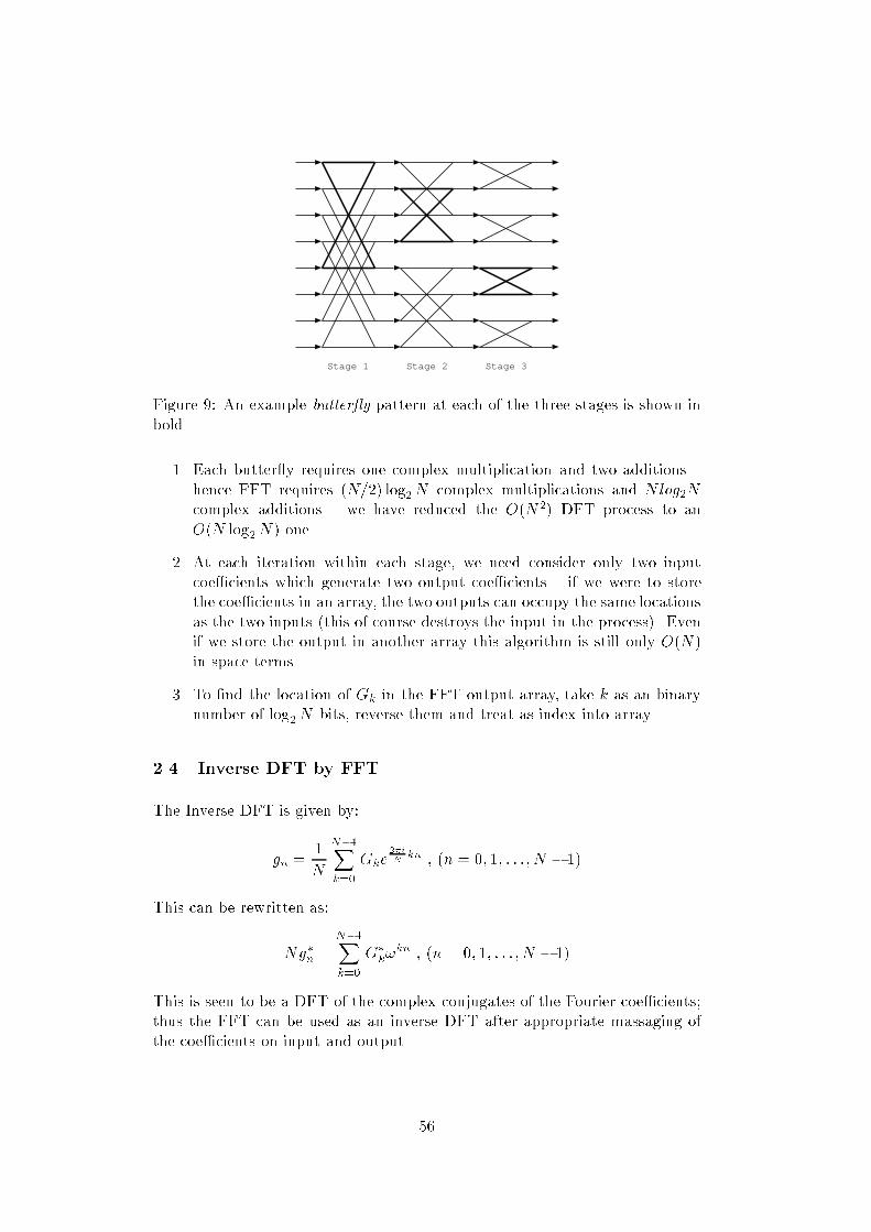
Stage 1 Stage 2 Stage 3Figure 9: An example butter y pattern at each of the three stages is shown inbold1. Each butter y requires one complex multiplication and two additions hence FFT requires (N=2) log2N complex multiplications and Nlog2Ncomplex additions we have reduced the O(N2) DFT process to anO(N log2N) one.2. At each iteration within each stage, we need consider only two inputcoecients which generate two output coecients if we were to storethe coecients in an array, the two outputs can occupy the same locationsas the two inputs (this of course destroys the input in the process). Evenif we store the output in another array this algorithm is still only O(N)in space terms.3. To nd the location of Gk in the FFT output array, take k as an binarynumber of log2N bits, reverse them and treat as index into array.2.4 Inverse DFT by FFTThe Inverse DFT is given by:gn = 1N N1Xk=0 Gke 2iN kn , (n = 0; 1; : : : ; N 1)This can be rewritten as:Ngn = N1Xk=0 Gk!kn , (n = 0; 1; : : : ; N 1)This is seen to be a DFT of the complex conjugates of the Fourier coecients;thus the FFT can be used as an inverse DFT after appropriate massaging ofthe coecients on input and output. 56

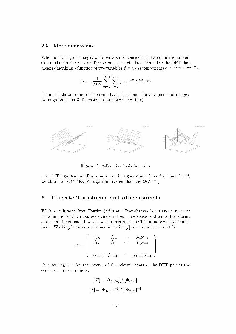
2.5 More dimensionsWhen operating on images, we often wish to consider the two dimensional ver-sion of the Fourier Series / Transform / Discrete Transform. For the DFT thatmeans describing a function of two variables f(x; y) as components e2i(nx=N+my=M):Fk;l = 1MN M1Xm=0 N1Xn=0 fm;ne2i(mkM +nlN )Figure 10 shows some of the cosine basis functions. For a sequence of images,we might consider 3 dimensions (two space, one time).cos(x)

01

23

45

6 01

23

45

6

-0.5

0

0.5

1

cos(y)

01

23

45

6 01

23

45

6

-0.5

0

0.5

1

cos(x)*cos(y)

01

23

45

6 01

23

45

6

-0.5

0

0.5

1Figure 10: 2-D cosine basis functionsThe FFT algorithm applies equally well in higher dimensions; for dimension d,we obtain an O(Nd logN) algorithm rather than the O(Nd+1).3 Discrete Transforms and other animalsWe have migrated from Fourier Series and Transforms of continuous space ortime functions which express signals in frequency space to discrete transformsof discrete functions. However, we can recast the DFT in a more general frame-work. Working in two dimensions, we write [f ] to represent the matrix:[f ] = 0BBBB@ f0;0 f0;1 f0;N1f1;0 f1;1 f1;N1... ...fM1;0 fM1;1 fM1;N1 1CCCCAthen writing []1 for the inverse of the relevant matrix, the DFT pair is theobvious matrix products: [F ] = [M;M ][f ][N;N][f ] = [M;M ]1[F ][N;N ]157

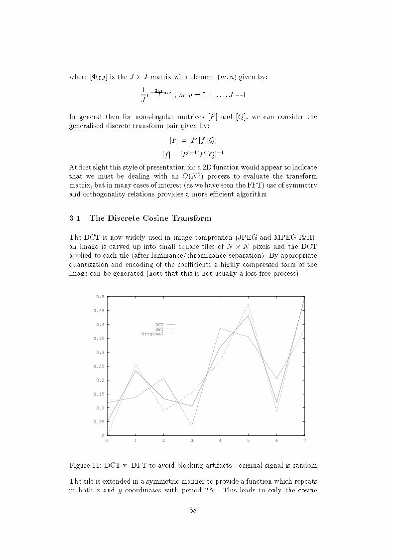
where [J;J ] is the J J matrix with element (m;n) given by:1J e 2iJ mn , m;n = 0; 1; : : : ; J 1In general then for non-singular matrices [P ] and [Q], we can consider thegeneralised discrete transform pair given by:[F ] = [P ][f ][Q][f ] = [P ]1[F ][Q]1At rst sight this style of presentation for a 2D function would appear to indicatethat we must be dealing with an O(N3) process to evaluate the transformmatrix, but in many cases of interest (as we have seen the FFT) use of symmetryand orthogonality relations provides a more ecient algorithm.3.1 The Discrete Cosine TransformThe DCT is now widely used in image compression (JPEG and MPEG I&II);an image is carved up into small square tiles of N N pixels and the DCTapplied to each tile (after luminance/chrominance separation). By appropriatequantization and encoding of the coecients a highly compressed form of theimage can be generated (note that this is not usually a loss free process).0

0.05

0.1

0.15

0.2

0.25

0.3

0.35

0.4

0.45

0.5

0 1 2 3 4 5 6 7

DCTDFT

Original

Figure 11: DCT v. DFT to avoid blocking artifacts - original signal is randomThe tile is extended in a symmetric manner to provide a function which repeatsin both x and y coordinates with period 2N . This leads to only the cosine58

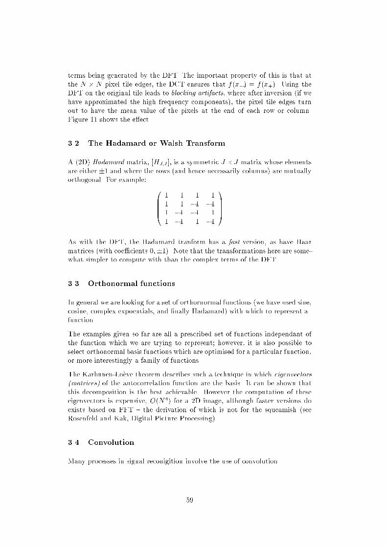
terms being generated by the DFT. The important property of this is that atthe N N pixel tile edges, the DCT ensures that f(x) = f(x+). Using theDFT on the original tile leads to blocking artifacts, where after inversion (if wehave approximated the high frequency components), the pixel tile edges turnout to have the mean value of the pixels at the end of each row or column.Figure 11 shows the eect.3.2 The Hadamard or Walsh TransformA (2D) Hadamard matrix, [HJ;J ], is a symmetric J J matrix whose elementsare either 1 and where the rows (and hence necessarily columns) are mutuallyorthogonal. For example: 0BBB@ 1 1 1 11 1 1 11 1 1 11 1 1 1 1CCCAAs with the DFT, the Hadamard tranform has a fast version, as have Haarmatrices (with coecients 0;1). Note that the transformations here are some-what simpler to compute with than the complex terms of the DFT.3.3 Orthonormal functionsIn general we are looking for a set of orthornormal functions (we have used sine,cosine, complex expoentials, and nally Hadamard) with which to represent afunction.The examples given so far are all a prescribed set of functions independant ofthe function which we are trying to represent; however, it is also possible toselect orthonormal basis functions which are optimised for a particular function,or more interestingly a family of functions.The Karhunen-Loeve theorem describes such a technique in which eigenvectors(matrices) of the autocorrelation function are the basis. It can be shown thatthis decomposition is the best achievable. However the computation of theseeigenvectors is expensive, O(N4) for a 2D image, although faster versions doexists based on FFT the derivation of which is not for the squeamish (seeRosenfeld and Kak, Digital Picture Processing).3.4 ConvolutionMany processes in signal reconigition involve the use of convolution.59

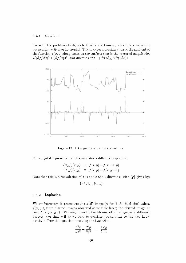
3.4.1 GradientConsider the problem of edge detection in a 2D image, where the edge is notnecessarily vertical or horizontal. This involves a consideration of the gradient ofthe function f(x; y) along paths on the surface; that is the vector of magnitude,p(@f=@x)2+ (@f=@y)2, and direction tan1((@f=@y)=(@f=@x)).-100

-50

0

50

100

150

200

0 50 100 150 200 250 300

functiongradient

Figure 12: 1D edge detection by convolutionFor a digital representation this indicates a dierence equation:(xf)(x; y) f(x; y) f(x 1; y)(yf)(x; y) f(x; y) f(x; y 1)Note that this is a convolution of f in the x and y directions with fgg given by:f1; 1; 0; 0; : : :g3.4.2 LaplacianWe are interested in reconstructing a 2D image (which had initial pixel valuesf(x; y)), from blurred images observed some time later; the blurred image attime t is g(x; y; t). We might model the bluring of an image as a diusionprocess over time if so we need to consider the solution to the well knowpartial dierential equation involving the Laplacian:@2g@x2 + @2g@y2 = 1k @g@t60

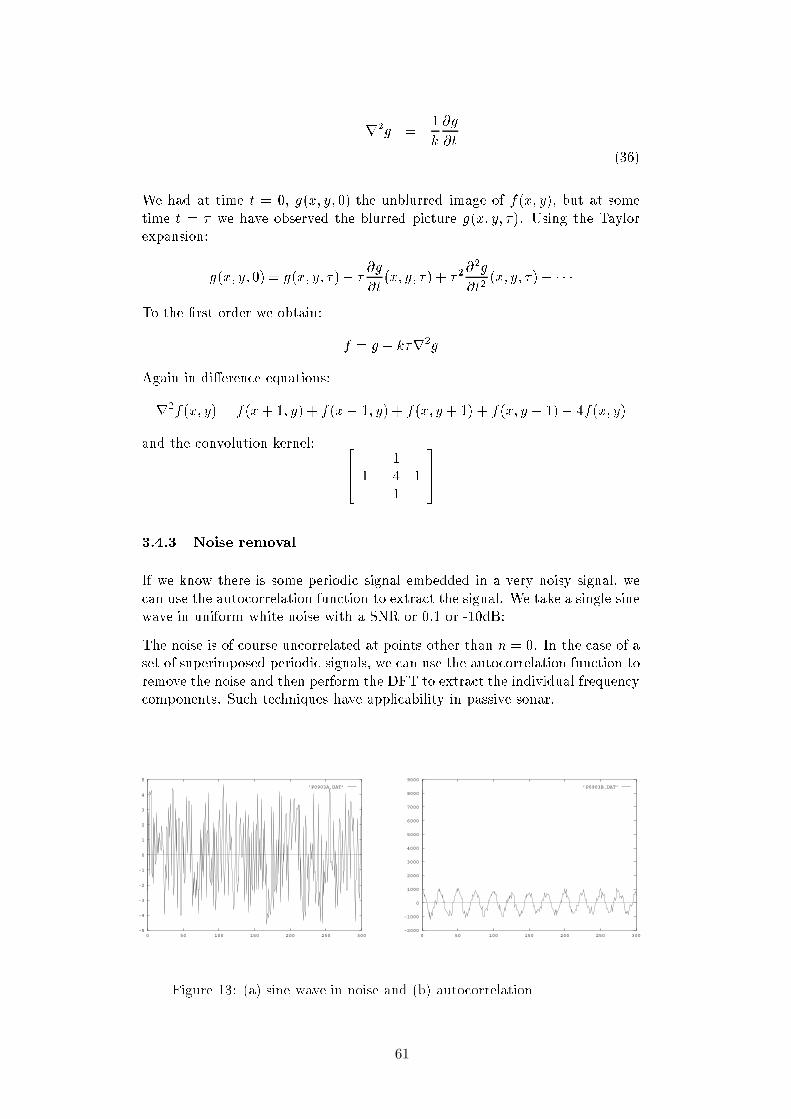
! #"$% &('*)' " +,-.,/,01-23245617897:;=< &('*)> $(/-,7?:>@31@ #ACBDFE:>/,?3G24E5H+,/,01-23245JI,LK5+-24 &('*)' A 5MON ?31.,8P*,QRFS,0L:>25TI.,?3L:>.VU

W&('+)X' " Y &%'+)X' A VZ A X &%'+)X' A X[ A X &('*)' A (Z6\G\F\Q%:7+,^]_24?3`:>24G2DBD:>/,+ .VU

<aY Z A7b 8>1.a1.adc(G24G.,K5e5fg-h:,.,?GU

< &('*)> i< &O[ '+),_[ < &Z '*)>X[ < &%'+)j[ %[ < W&('+)kZ lZm < W&('+),.,a+,eK5:>.9E:01-,3L:>.anG23.,50 U o

pq ZDm rtsu

v(wLxlw1v yazV|~PF~XPz;jBD7n>.,:B+,G27L?O?3:>!!IG24L:>LKa?3L8>.0G/551.E9G24S.,:L?3SC?3L8>.0 $(BDKG.7-,?j+,=-,:>K5:>2245013L:>.e;-.,K53L:>.3:5T>*23K5+,j?h8,.0 M j+9nj?31.,80L^?31.,BjFE=1.-.,t; :>23B=,L3O.,:L?3eBjL+=:>2D" M :,2 "^UQj,O.,:L?3^L?j:;RK5:,-24?3-.,K5:>232450135I:1.?j:+,G2+.ai" M .+,=KG?3=:;?35:;_?+-IG2417I:9?35IG24L:,LK?3L8>.0L?G$BDjKG9.7-,?3j+,^-,3:,K5:>23245013L:>.;W-.,K53L:>.3:24G@:E+,=.,:L?3^.,@+,G.7IG2;:>2+,D ¡¢Q3:5T,+23K5R+,` .,LE,L-0X;W245f-,G.,K5SK5:>7I:>.,G.93? M -,K5a35K5.,Lfg-,5?FEOII,0LLKG/,L0L14S1.I??3LEO?3:,.2 M

-5

-4

-3

-2

-1

0

1

2

3

4

5

0 50 100 150 200 250 300

’P0903A.DAT’

-2000

-1000

0

1000

2000

3000

4000

5000

6000

7000

8000

9000

0 50 100 150 200 250 300

’P0903B.DAT’

Figure a sine wave in noise and b autocorrelation

61

9 Quantized Degrees-of-Freedom in a Continuous Signal

We have now encountered several theorems expressing the idea that even though a signalis continuous and dense in time (i.e. the value of the signal is defined at each real-valuedmoment in time), nevertheless a finite and countable set of discrete numbers suffices todescribe it completely, and thus to reconstruct it, provided that its frequency bandwidth islimited.

Such theorems may seem counter-intuitive at first: How could a finite sequence of num-bers, at discrete intervals, capture exhaustively the continuous and uncountable stream ofnumbers that represent all the values taken by a signal over some interval of time?

In general terms, the reason is that bandlimited continuous functions are not as free tovary as they might at first seem. Consequently, specifying their values at only certainpoints, suffices to determine their values at all other points.

Three examples that we have already seen are:

• Nyquist’s Sampling Theorem: If a signal f(x) is strictly bandlimited so that itcontains no frequency components higher than W , i.e. its Fourier Transform F (k)satisfies the condition

F (k) = 0 for |k| > W (1)

then f(x) is completely determined just by sampling its values at a rate of at least2W . The signal f(x) can be exactly recovered by using each sampled value to fix theamplitude of a sinc(x) function,

sinc(x) =sin(πx)

πx(2)

whose width is scaled by the bandwidth parameter W and whose location correspondsto each of the sample points. The continuous signal f(x) can be perfectly recoveredfrom its discrete samples fn(nπ

W ) just by adding all of those displaced sinc(x) functionstogether, with their amplitudes equal to the samples taken:

f(x) =∑

n

fn

(

nπ

W

)

sin(Wx − nπ)

(Wx − nπ)(3)

Thus we see that any signal that is limited in its bandwidth to W , during someduration T has at most 2WT degrees-of-freedom. It can be completely specified byjust 2WT real numbers (Nyquist, 1911; R V Hartley, 1928).

• Logan’s Theorem: If a signal f(x) is strictly bandlimited to one octave or less, sothat the highest frequency component it contains is no greater than twice the lowestfrequency component it contains

kmax ≤ 2kmin (4)

i.e. F (k) the Fourier Transform of f(x) obeys

F (|k| > kmax = 2kmin) = 0 (5)

andF (|k| < kmin) = 0 (6)

and if it is also true that the signal f(x) contains no complex zeroes in common withits Hilbert Transform (too complicated to explain here, but this constraint serves to

62

exclude families of signals which are merely amplitude-modulated versions of eachother), then the original signal f(x) can be perfectly recovered (up to an amplitudescale constant) merely from knowledge of the set xi of zero-crossings of f(x) alone:

xi such that f(xi) = 0 (7)

Comments:(1) This is a very complicated, surprising, and recent result (W F Logan, 1977).

(2) Only an existence theorem has been proven. There is so far no stable constructivealgorithm for actually making this work – i.e. no known procedure that can actuallyrecover f(x) in all cases, within a scale factor, from the mere knowledge of its zero-crossings f(x) = 0; only the existence of such algorithms is proven.

(3) The “Hilbert Transform” constraint (where the Hilbert Transform of a signalis obtained by convolving it with a hyperbola, h(x) = 1/x, or equivalently by shiftingthe phase of the positive frequency components of the signal f(x) by +π/2 and shiftingthe phase of its negative frequency components by −π/2), serves to exclude ensem-bles of signals such as a(x) sin(ωx) where a(x) is a purely positive function a(x) > 0.Clearly a(x) modulates the amplitudes of such signals, but it could not change anyof their zero-crossings, which would always still occur at x = 0, π

ω , 2πω , 3π

ω , ..., and sosuch signals could not be uniquely represented by their zero-crossings.

(4) It is very difficult to see how to generalize Logan’s Theorem to two-dimensionalsignals (such as images). In part this is because the zero-crossings of two-dimensionalfunctions are non-denumerable (uncountable): they form continuous “snakes,” ratherthan a discrete and countable set of points. Also, it is not clear whether the one-octavebandlimiting constraint should be isotropic (the same in all directions), in which casethe projection of the signal’s spectrum onto either frequency axis is really low-passrather than bandpass; or anisotropic, in which case the projection onto both frequencyaxes may be strictly bandpass but the different directions are treated differently.

(5) Logan’s Theorem has been proposed as a significant part of a “brain theory”by David Marr and Tomaso Poggio, for how the brain’s visual cortex processes andinterprets retinal image information. The zero-crossings of bandpass-filtered retinalimages constitute edge information within the image.

• The Information Diagram: The Similarity Theorem of Fourier Analysis assertsthat if a function becomes narrower in one domain by a factor a, it necessarily becomesbroader by the same factor a in the other domain:

f(x) −→ F (k) (8)

f(ax) −→ |1a|F

(

k

a

)

(9)

The Hungarian Nobel-Laureate Dennis Gabor took this principle further with greatinsight and with implications that are still revolutionizing the field of signal processing(based upon wavelets), by noting that an Information Diagram representation of sig-nals in a plane defined by the axes of time and frequency is fundamentally quantized.There is an irreducible, minimal, area that any signal can possibly occupy in thisplane. Its uncertainty (or spread) in frequency, times its uncertainty (or duration) intime, has an inescapable lower bound.

63

10 Gabor-Heisenberg-Weyl Uncertainty Relation. “Logons.”

10.1 The Uncertainty Principle

If we define the “effective support” of a function f(x) by its normalized variance, or thenormalized second-moment:

(∆x)2 =

∫ +∞

−∞

f(x)f∗(x)(x − µ)2dx

∫ +∞

−∞

f(x)f∗(x)dx

(10)

where µ is the mean value, or normalized first-moment, of the function:

µ =

∫ +∞

−∞

xf(x)f∗(x)dx

∫ +∞

−∞

f(x)f∗(x)dx

(11)

and if we similarly define the effective support of the Fourier Transform F (k) of the functionby its normalized variance in the Fourier domain:

(∆k)2 =

∫ +∞

−∞

F (k)F ∗(k)(k − k0)2dk

∫ +∞

−∞

F (k)F ∗(k)dk

(12)

where k0 is the mean value, or normalized first-moment, of the Fourier transform F (k):

k0 =

∫ +∞

−∞

kF (k)F ∗(k)dk

∫ +∞

−∞

F (k)F ∗(k)dk

(13)

then it can be proven (by Schwartz Inequality arguments) that there exists a fundamentallower bound on the product of these two “spreads,” regardless of the function f(x):

(∆x)(∆k) ≥ 14π (14)

This is the famous Gabor-Heisenberg-Weyl Uncertainty Principle. Mathematically it isexactly identical to the uncertainty relation in quantum physics, where (∆x) would beinterpreted as the position of an electron or other particle, and (∆k) would be interpretedas its momentum or deBroglie wavelength. We see that this is not just a property of nature,but more abstractly a property of all functions and their Fourier Transforms. It is thus astill further respect in which the information in continuous signals is quantized, since theminimal area they can occupy in the Information Diagram has an irreducible lower bound.

10.2 Gabor “Logons”

Dennis Gabor named such minimal areas “logons” from the Greek word for information, or

order: logos. He thus established that the Information Diagram for any continuous signal

can only contain a fixed number of information “quanta.” Each such quantum constitutes

an independent datum, and their total number within a region of the Information Diagram

represents the number of independent degrees-of-freedom enjoyed by the signal.

64

The unique family of signals that actually achieve the lower bound in the Gabor-Heisenberg-

Weyl Uncertainty Relation are the complex exponentials multiplied by Gaussians. These

are sometimes referred to as “Gabor wavelets:”

f(x) = e−(x−x0)2/a2

e−ik0(x−x0) (15)

localized at “epoch” x0, modulated by frequency k0, and with size or spread constant a.

It is noteworthy that such wavelets have Fourier Transforms F (k) with exactly the same

functional form, but with their parameters merely interchanged or inverted:

F (k) = e−(k−k0)2a2

eix0(k−k0) (16)

Note that in the case of a wavelet (or wave-packet) centered on x0 = 0, its Fourier Trans-form is simply a Gaussian centered at the modulation frequency k0, and whose size is 1/a,the reciprocal of the wavelet’s space constant.

Because of the optimality of such wavelets under the Uncertainty Principle, Gabor (1946)proposed using them as an expansion basis to represent signals. In particular, he wantedthem to be used in broadcast telecommunications for encoding continuous-time informa-tion. He called them the “elementary functions” for a signal. Unfortunately, because suchfunctions are mutually non-orthogonal, it is very difficult to obtain the actual coefficientsneeded as weights on the elementary functions in order to expand a given signal in thisbasis. The first constructive method for finding such “Gabor coefficients” was developedin 1981 by the Dutch physicist Martin Bastiaans, using a dual basis and a complicatednon-local infinite series.

The following diagrams show the behaviour of Gabor elementary functions both as complexwavelets, their separate real and imaginary parts, and their Fourier transforms. When afamily of such functions are parameterized to be self-similar, i.e. they are dilates and trans-lates of each other so that they all have a common template (“mother” and “daughter”),then they constitute a (non-orthogonal) wavelet basis. Today it is known that an infiniteclass of wavelets exist which can be used as the expansion basis for signals. Because ofthe self-similarity property, this amounts to representing or analyzing a signal at differentscales. This general field of investigation is called multi-resolution analysis.

65

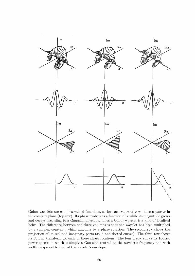
Gabor wavelets are complex-valued functions, so for each value of x we have a phasor inthe complex plane (top row). Its phase evolves as a function of x while its magnitude growsand decays according to a Gaussian envelope. Thus a Gabor wavelet is a kind of localisedhelix. The difference between the three columns is that the wavelet has been multipliedby a complex constant, which amounts to a phase rotation. The second row shows theprojection of its real and imaginary parts (solid and dotted curves). The third row showsits Fourier transform for each of these phase rotations. The fourth row shows its Fourierpower spectrum which is simply a Gaussian centred at the wavelet’s frequency and withwidth reciprocal to that of the wavelet’s envelope.

66

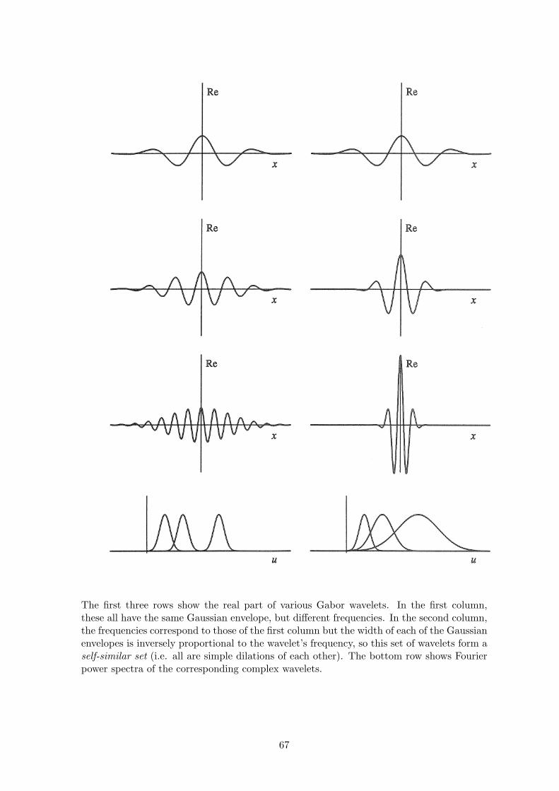
The first three rows show the real part of various Gabor wavelets. In the first column,these all have the same Gaussian envelope, but different frequencies. In the second column,the frequencies correspond to those of the first column but the width of each of the Gaussianenvelopes is inversely proportional to the wavelet’s frequency, so this set of wavelets form aself-similar set (i.e. all are simple dilations of each other). The bottom row shows Fourierpower spectra of the corresponding complex wavelets.

67

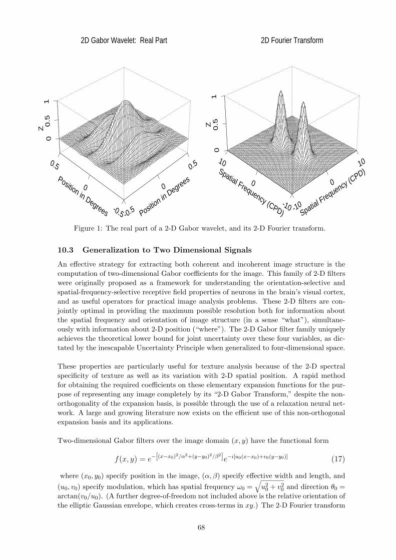
-0.5

0

0.5

Position in Degrees

-0.5

0

0.5

Position in Degrees

00.5

1Z

2D Gabor Wavelet: Real Part

-10

0

10

Spatial Frequency (CPD)

-10

0

10Spatial Frequency (CPD)

00.5

1Z

2D Fourier Transform

Figure 1: The real part of a 2-D Gabor wavelet, and its 2-D Fourier transform.

10.3 Generalization to Two Dimensional Signals

An effective strategy for extracting both coherent and incoherent image structure is the

computation of two-dimensional Gabor coefficients for the image. This family of 2-D filters

were originally proposed as a framework for understanding the orientation-selective and

spatial-frequency-selective receptive field properties of neurons in the brain’s visual cortex,

and as useful operators for practical image analysis problems. These 2-D filters are con-

jointly optimal in providing the maximum possible resolution both for information about

the spatial frequency and orientation of image structure (in a sense “what”), simultane-

ously with information about 2-D position (“where”). The 2-D Gabor filter family uniquely

achieves the theoretical lower bound for joint uncertainty over these four variables, as dic-

tated by the inescapable Uncertainty Principle when generalized to four-dimensional space.

These properties are particularly useful for texture analysis because of the 2-D spectral

specificity of texture as well as its variation with 2-D spatial position. A rapid method

for obtaining the required coefficients on these elementary expansion functions for the pur-

pose of representing any image completely by its “2-D Gabor Transform,” despite the non-

orthogonality of the expansion basis, is possible through the use of a relaxation neural net-

work. A large and growing literature now exists on the efficient use of this non-orthogonal

expansion basis and its applications.

Two-dimensional Gabor filters over the image domain (x, y) have the functional form

f(x, y) = e−[(x−x0)2/α2+(y−y0)2/β2]e−i[u0(x−x0)+v0(y−y0)] (17)

where (x0, y0) specify position in the image, (α, β) specify effective width and length, and

(u0, v0) specify modulation, which has spatial frequency ω0 =√

u20 + v2

0 and direction θ0 =

arctan(v0/u0). (A further degree-of-freedom not included above is the relative orientation of

the elliptic Gaussian envelope, which creates cross-terms in xy.) The 2-D Fourier transform

68

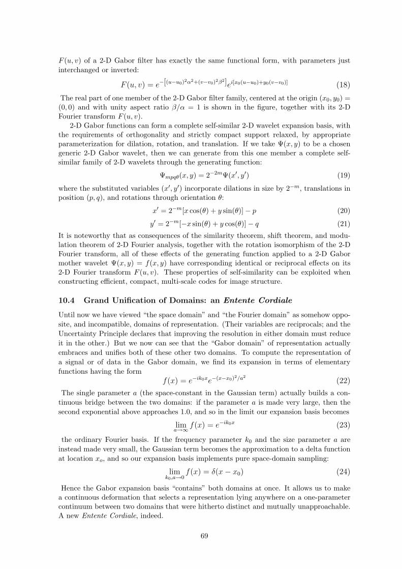
F (u, v) of a 2-D Gabor filter has exactly the same functional form, with parameters just

interchanged or inverted:

F (u, v) = e−[(u−u0)2α2+(v−v0)2β2]ei[x0(u−u0)+y0(v−v0)] (18)

The real part of one member of the 2-D Gabor filter family, centered at the origin (x0, y0) =(0, 0) and with unity aspect ratio β/α = 1 is shown in the figure, together with its 2-DFourier transform F (u, v).

2-D Gabor functions can form a complete self-similar 2-D wavelet expansion basis, withthe requirements of orthogonality and strictly compact support relaxed, by appropriateparameterization for dilation, rotation, and translation. If we take Ψ(x, y) to be a chosengeneric 2-D Gabor wavelet, then we can generate from this one member a complete self-similar family of 2-D wavelets through the generating function:

Ψmpqθ(x, y) = 2−2mΨ(x′, y′) (19)

where the substituted variables (x′, y′) incorporate dilations in size by 2−m, translations inposition (p, q), and rotations through orientation θ:

x′ = 2−m[x cos(θ) + y sin(θ)] − p (20)

y′ = 2−m[−x sin(θ) + y cos(θ)] − q (21)

It is noteworthy that as consequences of the similarity theorem, shift theorem, and modu-lation theorem of 2-D Fourier analysis, together with the rotation isomorphism of the 2-DFourier transform, all of these effects of the generating function applied to a 2-D Gabormother wavelet Ψ(x, y) = f(x, y) have corresponding identical or reciprocal effects on its2-D Fourier transform F (u, v). These properties of self-similarity can be exploited whenconstructing efficient, compact, multi-scale codes for image structure.

10.4 Grand Unification of Domains: an Entente Cordiale

Until now we have viewed “the space domain” and “the Fourier domain” as somehow oppo-

site, and incompatible, domains of representation. (Their variables are reciprocals; and the

Uncertainty Principle declares that improving the resolution in either domain must reduce

it in the other.) But we now can see that the “Gabor domain” of representation actually

embraces and unifies both of these other two domains. To compute the representation of

a signal or of data in the Gabor domain, we find its expansion in terms of elementary

functions having the form

f(x) = e−ik0xe−(x−x0)2/a2

(22)

The single parameter a (the space-constant in the Gaussian term) actually builds a con-

tinuous bridge between the two domains: if the parameter a is made very large, then the

second exponential above approaches 1.0, and so in the limit our expansion basis becomes

lima→∞

f(x) = e−ik0x (23)

the ordinary Fourier basis. If the frequency parameter k0 and the size parameter a are

instead made very small, the Gaussian term becomes the approximation to a delta function

at location xo, and so our expansion basis implements pure space-domain sampling:

limk0,a→0

f(x) = δ(x − x0) (24)

Hence the Gabor expansion basis “contains” both domains at once. It allows us to makea continuous deformation that selects a representation lying anywhere on a one-parametercontinuum between two domains that were hitherto distinct and mutually unapproachable.A new Entente Cordiale, indeed.

69

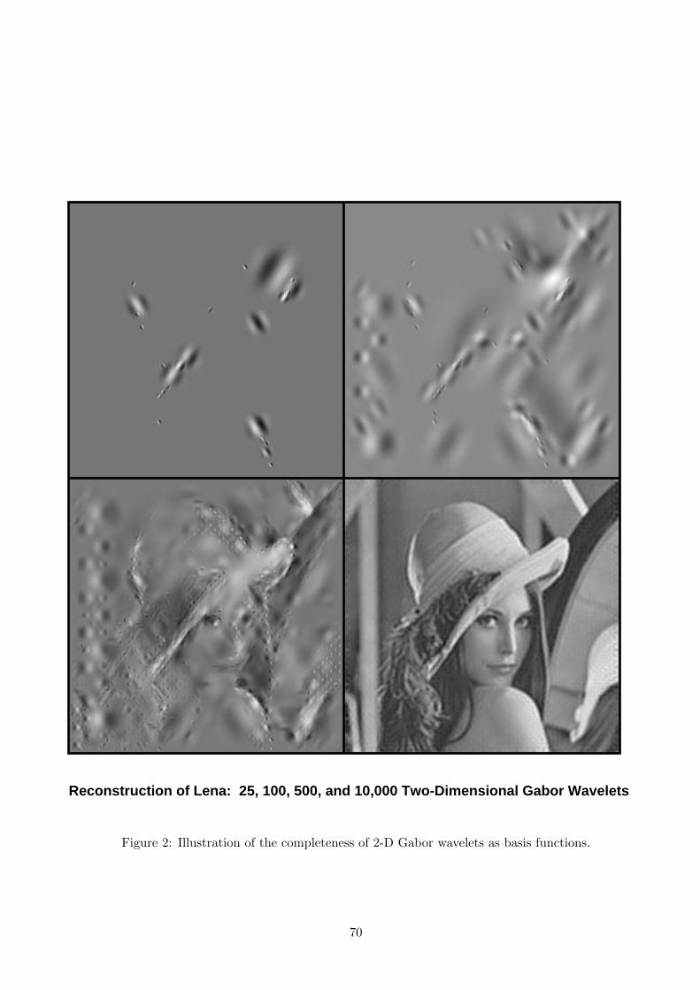
Reconstruction of Lena: 25, 100, 500, and 10,000 Two-Dimensional Gabor Wavelets

Figure 2: Illustration of the completeness of 2-D Gabor wavelets as basis functions.

70

11 Kolmogorov Complexity and Minimal Description Length

An idea of fundamental importance is the measure known as Kolmogorov complexity: thecomplexity of a string of data is defined as the length of the shortest binary program forcomputing the string. Thus the complexity is the data’s “minimal description length.”

It is an amazing fact that the Kolmogorov complexity K of a string is approximatelyequal to the entropy H of the distribution from which the string is a randomly drawnsequence. Thus Kolmogorov descriptive complexity is intimately connected with informa-tion theory, and indeed K defines the ultimate data compression. Reducing the data to aprogram that generates it exactly is obviously a way of compressing it; and running thatprogram is a way of decompressing it. Any set of data can be generated by a computerprogram, even if (in the worst case) that program simply consists of data statements. Thelength of such a program defines its algorithmic complexity.

It is important to draw a clear distinction between the notions of computational com-

plexity (measured by program execution time), and algorithmic complexity (measured byprogram length). Kolmogorov complexity is concerned with finding descriptions whichminimize the latter. Little is known about how (in analogy with the optimal propertiesof Gabor’s elementary logons in the 2D Information Plane) one might try to minimizesimultaneously along both of these orthogonal axes that form a “Complexity Plane.”

Most sequences of length n (where “most” considers all possible permutations of nbits) have Kolmogorov complexity K close to n. The complexity of a truly random binarysequence is as long as the sequence itself. However, it is not clear how to be certain ofdiscovering that a given string has a much lower complexity than its length. It might beclear that the string

0101010101010101010101010101010101010101010101010101010101010101

has a complexity much less than 32 bits; indeed, its complexity is the length of the program:Print 32 "01"s. But consider the string

0110101000001001111001100110011111110011101111001100100100001000

which looks random and passes most tests for randomness. How could you discover thatthis sequence is in fact just the binary expansion for the irrational number

√2−1, and that

therefore it can be specified extremely concisely?Fractals are examples of entities that look very complex but in fact are generated by

very simple programs (i.e. iterations of a mapping). Therefore, the Kolmogorov complexityof fractals is nearly zero.

A sequence x1, x2, x3, ..., xn of length n is said to be algorithmically random if its Kol-mogorov complexity is at least n (i.e. the shortest possible program that can generate thesequence is a listing of the sequence itself):

K(x1x2x3...xn|n) ≥ n (25)

An infinite string is defined to be incompressible if its Kolmogorov complexity, in the limitas the string gets arbitrarily long, approaches the length n of the string itself:

limn→∞

K(x1x2x3...xn|n)

n= 1 (26)

An interesting theorem, called the Strong Law of Large Numbers for Incompressible Se-

quences, asserts that the proportions of 0’s and 1’s in any incompressible string must benearly equal! Moreover, any incompressible sequence must satisfy all computable statistical

71

tests for randomness. (Otherwise, identifying the statistical test for randomness that thestring failed would reduce the descriptive complexity of the string, which contradicts itsincompressibility.) Therefore the algorithmic test for randomness is the ultimate test, sinceit includes within it all other computable tests for randomness.

12 A Short Bibliography

Cover, T M and Thomas, J A (1991) Elements of Information Theory. New York: Wiley.

Blahut, R E (1987) Principles and Practice of Information Theory. New York: Addison-Wesley.

Bracewell, R (1995) The Fourier Transform and its Applications. New York: McGraw-Hill.

Fourier analysis: besides the above, an excellent on-line tutorial is available at:http://users.ox.ac.uk/˜ball0597/Fourier/

McEliece, R J (1977) The Theory of Information and Coding: A Mathematical Framework

for Communication. Addison-Wesley. Reprinted (1984) by Cambridge University Press inEncyclopedia of Mathematics.

McMullen, C W (1968) Communication Theory Principles. New York: MacMillan.

Shannon, C and Weaver, W (1949) Mathematical Theory of Communication. Urbana:University of Illinois Press.

Wiener, N (1948) Time Series. Cambridge: MIT Press.

72