Coding TheoryA First Course

Coding theory is concerned with successfully transmitting data through a noisychannel and correcting errors in corrupted messages. It is of central importance formany applications in computer science or engineering. This book gives acomprehensive introduction to coding theory whilst only assuming basic linearalgebra. It contains a detailed and rigorous introduction to the theory of block codesand moves on to more advanced topics such as BCH codes, Goppa codes and Sudan’salgorithm for list decoding. The issues of bounds and decoding, essential to the designof good codes, feature prominently.

The authors of this book have, for several years, successfully taught a course on codingtheory to students at the National University of Singapore. This book is based on theirexperiences and provides a thoroughly modern introduction to the subject. There is awealth of examples and exercises, some of which introduce students to novel or moreadvanced material.

Coding TheoryA First Course

SAN LINGCHAOPING XING

National University of Singapore

Cambridge, New York, Melbourne, Madrid, Cape Town, Singapore, São Paulo

Cambridge University PressThe Edinburgh Building, Cambridge , UK

First published in print format

- ----

- ----

- ----

© Cambridge University Press 2004

2004

Information on this title: www.cambridge.org/9780521821919

This publication is in copyright. Subject to statutory exception and to the provision ofrelevant collective licensing agreements, no reproduction of any part may take placewithout the written permission of Cambridge University Press.

- ---

- ---

- ---

Cambridge University Press has no responsibility for the persistence or accuracy of sfor external or third-party internet websites referred to in this publication, and does notguarantee that any content on such websites is, or will remain, accurate or appropriate.

Published in the United States of America by Cambridge University Press, New York

www.cambridge.org

hardback

paperback

paperback

eBook (EBL)

eBook (EBL)

hardback

Contents

Preface page xi

1 Introduction 1Exercises 4

2 Error detection, correction and decoding 52.1 Communication channels 52.2 Maximum likelihood decoding 82.3 Hamming distance 82.4 Nearest neighbour/minimum distance decoding 102.5 Distance of a code 11

Exercises 14

3 Finite fields 173.1 Fields 173.2 Polynomial rings 223.3 Structure of finite fields 263.4 Minimal polynomials 30

Exercises 36

4 Linear codes 394.1 Vector spaces over finite fields 394.2 Linear codes 454.3 Hamming weight 464.4 Bases for linear codes 484.5 Generator matrix and parity-check matrix 524.6 Equivalence of linear codes 564.7 Encoding with a linear code 574.8 Decoding of linear codes 59

vii

viii Contents

4.8.1 Cosets 594.8.2 Nearest neighbour decoding for linear codes 614.8.3 Syndrome decoding 62

Exercises 66

5 Bounds in coding theory 755.1 The main coding theory problem 755.2 Lower bounds 805.2.1 Sphere-covering bound 805.2.2 Gilbert–Varshamov bound 825.3 Hamming bound and perfect codes 835.3.1 Binary Hamming codes 845.3.2 q-ary Hamming codes 875.3.3 Golay codes 885.3.4 Some remarks on perfect codes 925.4 Singleton bound and MDS codes 925.5 Plotkin bound 955.6 Nonlinear codes 965.6.1 Hadamard matrix codes 985.6.2 Nordstrom–Robinson code 985.6.3 Preparata codes 995.6.4 Kerdock codes 995.7 Griesmer bound 1005.8 Linear programming bound 102

Exercises 106

6 Constructions of linear codes 1136.1 Propagation rules 1136.2 Reed–Muller codes 1186.3 Subfield codes 121

Exercises 126

7 Cyclic codes 1337.1 Definitions 1337.2 Generator polynomials 1367.3 Generator and parity-check matrices 1417.4 Decoding of cyclic codes 1457.5 Burst-error-correcting codes 150

Exercises 153

Contents ix

8 Some special cyclic codes 1598.1 BCH codes 1598.1.1 Definitions 1598.1.2 Parameters of BCH codes 1618.1.3 Decoding of BCH codes 1688.2 Reed–Solomon codes 1718.3 Quadratic-residue codes 175

Exercises 183

9 Goppa codes 1899.1 Generalized Reed–Solomon codes 1899.2 Alternant codes 1929.3 Goppa codes 1969.4 Sudan decoding for generalized RS codes 2029.4.1 Generation of the (P, k, t)-polynomial 2039.4.2 Factorization of the (P, k, t)-polynomial 205

Exercises 209

References 215Bibliography 217Index 219

Preface

In the seminal paper ‘A mathematical theory of communication’ published in1948, ClaudeShannon showed that, given anoisy communication channel, thereis a number, called the capacity of the channel, such that reliable communicationcan be achieved at any rate below the channel capacity, if proper encoding anddecoding techniques are used. This marked the birth of coding theory, a fieldof study concerned with the transmission of data across noisy channels and therecovery of corrupted messages.In barely more than half a century, coding theory has seen phenomenal

growth. It has found widespread application in areas ranging from communi-cation systems, to compact disc players, to storage technology. In the effort tofind good codes for practical purposes, researchers have moved beyond blockcodes to other paradigms, such as convolutional codes, turbo codes, space-timecodes, low-density-parity-check (LDPC) codes and even quantumcodes. Whilethe problems in coding theory often arise from engineering applications, it isfascinating to note the crucial role played by mathematics in the developmentof the field. The importance of algebra, combinatorics and geometry in codingtheory is a commonly acknowledged fact, with many deepmathematical resultsbeing used in elegant ways in the advancement of coding theory.Coding theory therefore appeals not just to engineers and computer scien-

tists, but also tomathematicians. It has become increasingly common to find thesubject taught as part of undergraduate or graduate curricula in mathematics.This book grew out of two one-semester courses we have taught at the

National University of Singapore to advanced mathematics and computerscience undergraduates over a number of years. Given the vastness of thesubject, we have chosen to restrict our attention to block codes, with the aimof introducing the theory without a prerequisite in algebra. The only mathe-matical prerequisite assumed is familiarity with basic notions and results in

xi

xii Preface

linear algebra. The results on finite fields needed in the book are covered inChapter 3.The design of good codes, from both the theoretical and practical points of

view, is a very important problem in coding theory. General bounds on theparameters of codes are often used as benchmarks to determine how good agiven code is, while, from the practical perspective, a code must admit an effi-cient decoding scheme before it can be considered useful. Since the beginningof coding theory, researchers have done much work in these directions and, inthe process, have constructed many interesting families of codes. This book isbuilt pretty much around these themes. A fairly detailed discussion on somewell known bounds is included in Chapter 5, while quite a number of decodingtechniques are discussed throughout this book. An effort is also made to in-troduce systematically many of the well known families of codes, for example,Hamming codes, Golay codes, Reed–Muller codes, cyclic codes, BCH codes,Reed–Solomon codes, alternant codes, Goppa codes, etc.In order to stay sufficiently focused and to keep the bookwithin amanageable

size, we have to omit certain well established topics or examples, such as athorough treatment of weight enumerators, from our discussion. Whereverpossible, we try to include some of these omitted topics in the exercises atthe end of each chapter. More than 250 problems have been included to helpstrengthen the reader’s understanding and to serve as an additional source ofexamples and results.Finally, it is a pleasure for us to acknowledge the help we have received

while writing this book. Our research work in coding theory has receivedgenerous financial assistance from the Ministry of Education (Singapore), theNational University of Singapore, the Defence Science and TechnologyAgency (Singapore) and the Chinese Academy of Sciences. We are thank-ful to these organizations for their support. We thank those who have readthrough the drafts carefully and provided us with invaluable feedback, espe-cially Fangwei Fu, Wilfried Meidl, Harald Niederreiter, Yuansheng Tang (whohas also offered us generous help in the preparation of Section 9.4), ArneWinterhof and Sze Ling Yeo, as well as the students in the classes MA3218andMA4261. David Chew has been most helpful in assisting us with problemsconcerning LATEX, and we are most grateful for his help. We would also like tothank Shanthi d/o Devadas for secretarial help.

1 Introduction

Information media, such as communication systems and storage devices ofdata, are not absolutely reliable in practice because of noise or other formsof introduced interference. One of the tasks in coding theory is to detect, oreven correct, errors. Usually, coding is defined as source coding and channelcoding. Source coding involves changing the message source to a suitablecode to be transmitted through the channel. An example of source coding isthe ASCII code, which converts each character to a byte of 8 bits. A simplecommunication model can be represented by Fig. 1.1.

Example 1.0.1 Consider the source encoding of four fruits, apple, banana,cherry, grape, as follows:

apple → 00, banana → 01, cherry → 10, grape → 11.

Suppose the message ‘apple’, which is encoded as 00, is transmitted over anoisy channel. The message may become distorted and may be received as 01(see Fig. 1.2). The receiver may not realize that the message was corrupted.This communication fails.

The idea of channel coding is to encode the message again after the sourcecoding by introducing some form of redundancy so that errors can be detectedor even corrected. Thus, Fig. 1.1 becomes Fig. 1.3.

message source receiver

↓ ↑source encoder −→ channel −→ source decoder

Fig. 1.1.

1

2 Introduction

apple banana

↓ ↑00 −→ channel −→ 01

↑noise

Fig. 1.2.

message source receiver

↓ ↑source encoder source decoder

↓ ↑channel encoder −→ channel −→ channel decoder

Fig. 1.3.

Example 1.0.2 In Example 1.0.1, we perform the channel encoding by intro-ducing a redundancy of 1 bit as follows:

00 → 000, 01 → 011, 10 → 101, 11 → 110.

Suppose that the message ‘apple’, which is encoded as 000 after the sourceand channel encoding, is transmitted over a noisy channel, and that there is onlyone error introduced. Then the received word must be one of the following three:100, 010 or 001. In this way, we can detect the error, as none of 100, 010 or001 is among our encoded messages.

Note that the above encoding scheme allows us to detect errors at the costof reducing transmission speed as we have to transmit 3 bits for a message of2 bits.

The above channel encoding scheme does not allow us to correct errors. Forinstance, if 100 is received, then we do not know whether 100 comes from 000,110 or 101. However, if more redundancy is introduced, we are able to correcterrors. For instance, we can design the following channel coding scheme:

00 → 00000, 01 → 01111, 10 → 10110, 11 → 11001.

Suppose that the message ‘apple’ is transmitted over a noisy channel, and thatthere is only one error introduced. Then the received word must be one of thefollowing five: 10000, 01000, 00100, 00010 or 00001. Assume that 10000 isreceived. Then we can be sure that 10000 comes from 00000 because there are

Introduction 3

apple apple

↓ ↑00 00000↓ ↑

00000 −→ channel −→ 10000↑

noise

Fig. 1.4.

at least two errors between 10000 and each of the other three encoded messages01111, 10110 and 11001.

Note that we lose even more in terms of information transmission speed inthis case.

See Fig. 1.4 for this example.

Example 1.0.3 Here is a simple and general method of adding redundancy forthe purpose of error correction. Assume that source coding has already beendone and that the information consists of bit strings of fixed length k. Encodingis carried out by taking a bit string and repeating it 2r + 1 times, where r ≥ 1is a fixed integer. For instance,

01 −→ 0101010101

if k = 2 and r = 2. In this special case, decoding is done by first consideringthe positions 1, 3, 5, 7, 9 of the received string and taking the first decoded bitas the one which appears more frequently at these positions; we deal similarlywith the positions 2, 4, 6, 8, 10 to obtain the second decoded bit. For instance,the received string

1100100010

is decoded to 10. It is clear that, in this special case, we can decode up to twoerrors correctly. In the general case, we can decode up to r errors correctly.Since r is arbitrary, there are thus encoders which allow us to correct as manyerrors as we want. For obvious reasons, this method is called a repetitioncode. The only problem with this method is that it involves a serious loss ofinformation transmission speed. Thus, we will look for more efficient methods.

The goal of channel coding is to construct encoders and decoders in such away as to effect:

(1) fast encoding of messages;

4 Introduction

(2) easy transmission of encoded messages;(3) fast decoding of received messages;(4) maximum transfer of information per unit time;(5) maximal detection or correction capability.

From the mathematical point of view, the primary goals are (4) and (5).However, (5) is, in general, not compatible with (4), as we will see in Chapter 5.Therefore, any solution is necessarily a trade-off among the five objectives.

Throughout this book, we are primarily concerned with channel coding.Channel coding is also called algebraic coding as algebraic tools are extensivelyinvolved in the study of channel coding.

Exercises

1.1 Design a channel coding scheme to detect two or less errors for the messagesource {00, 10, 01, 11}. Can you find one of the best schemes in terms ofinformation transmission speed?

1.2 Design a channel coding scheme to correct two or less errors for themessage source {00, 10, 01, 11}. Can you find one of the best schemesin terms of information transmission speed?

1.3 Design a channel coding scheme to detect one error for the message source

{000, 100, 010, 001, 110, 101, 011, 111}.Can you find one of the best schemes in terms of information transmissionspeed?

1.4 Design a channel coding scheme to correct one error for the message source

{000, 100, 010, 001, 110, 101, 011, 111}.Can you find one of the best schemes in terms of information transmissionspeed?

2 Error detection, correctionand decoding

We saw in Chapter 1 that the purpose of channel coding is to introduce redun-dancy to information messages so that errors that occur in the transmission canbe detected or even corrected. In this chapter, we formalize and discuss thenotions of error-detection and error-correction. We also introduce some wellknown decoding rules, i.e., methods that retrieve the original message sent bydetecting and correcting the errors that have occurred in the transmission.

2.1 Communication channels

We begin with some basic definitions.

Definition 2.1.1 Let A = {a1, a2, . . . , aq} be a set of size q, which we refer toas a code alphabet and whose elements are called code symbols.

(i) A q-ary word of length n over A is a sequence w = w1w2 · · · wn witheach wi ∈ A for all i . Equivalently, w may also be regarded as the vector(w1, . . . , wn).

(ii) A q-ary block code of length n over A is a nonempty set C of q-ary wordshaving the same length n.

(iii) An element of C is called a codeword in C .(iv) The number of codewords in C , denoted by |C |, is called the size of C .(v) The (information) rate of a code C of length n is defined to be (logq |C |)/n.

(vi) A code of length n and size M is called an (n, M)-code.

Remark 2.1.2 In practice, and especially in this book, the code alphabet isoften taken to be a finite field Fq of order q (cf. Chapter 3).

5

6 Error detection, correction and decoding

a1 � � a1

a2 � � a2

� �

P(a j | ai )ai � � � a j

� �

aq � � aq

Fig. 2.1.

Example 2.1.3 A code over the code alphabet F2 = {0, 1} is called a binarycode; i.e., the code symbols for a binary code are 0 and 1. Some examples ofbinary codes are:

(i) C1 = {00, 01, 10, 11} is a (2,4)-code;(ii) C2 = {000, 011, 101, 110} is a (3,4)-code;

(iii) C3 = {0011, 0101, 1010, 1100, 1001, 0110} is a (4,6)-code.

A code over the code alphabet F3 = {0, 1, 2} is called a ternary code, whilethe term quaternary code is sometimes used for a code over the code alphabetF4. However, a code over the code alphabet Z4 = {0, 1, 2, 3} is also sometimesreferred to as a quaternary code (cf. Chapter 3 for the definitions of F3, F4

and Z4).

Definition 2.1.4 A communication channel consists of a finite channel al-phabet A = {a1, . . . , aq} as well as a set of forward channel probabilitiesP(a j received | ai sent), satisfying

q∑j=1

P(a j received | ai sent) = 1

for all i (see Fig. 2.1). (Here, P(a j received | ai sent) is the conditional proba-bility that a j is received, given that ai is sent.)

Definition 2.1.5 A communication channel is said to be memoryless if theoutcome of any one transmission is independent of the outcome of the previoustransmissions; i.e., if c = c1c2 · · · cn and x = x1x2 · · · xn are words of length n,then

P(x received | c sent) =n∏

i=1

P(xi received | ci sent).

2.1 Communication channels 7

0 � � � 01 − p

1 − p

p

p

��

��

��

����

��

��

��1 � � � 1

Fig. 2.2. Binary symmetric channel.

Definition 2.1.6 A q-ary symmetric channel is a memoryless channel whichhas a channel alphabet of size q such that

(i) each symbol transmitted has the same probability p (<1/2) of being re-ceived in error;

(ii) if a symbol is received in error, then each of the q − 1 possible errors isequally likely.

In particular, the binary symmetric channel (BSC ) is a memoryless channelwhich has channel alphabet {0, 1} and channel probabilities

P(1 received | 0 sent) = P(0 received | 1 sent) = p,

P(0 received | 0 sent) = P(1 received | 1 sent) = 1 − p.

Thus, the probability of a bit error in a BSC is p. This is called the crossoverprobability of the BSC (see Fig. 2.2).

Example 2.1.7 Suppose that codewords from the code {000, 111} are beingsent over a BSC with crossover probability p = 0.05. Suppose that the word110 is received. We can try to find the more likely codeword sent by computingthe forward channel probabilities:

P(110 received | 000 sent) = P(1 received | 0 sent)2 × P(0 received | 0 sent)

= (0.05)2(0.95) = 0.002375,

P(110 received | 111 sent) = P(1 received | 1 sent)2 × P(0 received | 1 sent)

= (0.95)2(0.05) = 0.045125.

Since the second probability is larger than the first, we can conclude that 111is more likely to be the codeword sent.

8 Error detection, correction and decoding

Decoding ruleIn a communication channel with coding, only codewords are transmitted.Suppose that a word w is received. If w is a valid codeword, we may concludethat there is no error in the transmission. Otherwise, we know that some errorshave occurred. In this case, we need a rule for finding the most likely codewordsent. Such a rule is known as a decoding rule. We discuss two such generalrules in this chapter. Some other decoding rules, which may apply to certainspecific families of codes, will also be introduced in subsequent chapters.

2.2 Maximum likelihood decoding

Suppose that codewords from a code C are being sent over a communicationchannel. If a word x is received, we can compute the forward channel proba-bilities

P(x received | c sent)

for all the codewords c ∈ C . The maximum likelihood decoding (MLD) rulewill conclude that cx is the most likely codeword transmitted if cx maximizesthe forward channel probabilities; i.e.,

P(x received | cx sent) = maxc∈C

P(x received | c sent).

There are two kinds of MLD:

(i) Complete maximum likelihood decoding (CMLD). If a word x is received,find the most likely codeword transmitted. If there are more than one suchcodewords, select one of them arbitrarily.

(ii) Incomplete maximum likelihood decoding (IMLD). If a word x is received,find the most likely codeword transmitted. If there are more than one suchcodewords, request a retransmission.

2.3 Hamming distance

Suppose that codewords from a code C are being sent over a BSC with crossoverprobability p < 1/2 (in practice, p should be much smaller than 1/2). If a wordx is received, then for any codeword c ∈ C the forward channel probability isgiven by

P(x received | c sent) = pe(1 − p)n−e,

where n is the length of x and e is the number of places at which x and c differ.Since p < 1/2, it follows that 1 − p > p, so this probability is larger for

2.3 Hamming distance 9

larger values of n − e, i.e., for smaller values of e. Hence, this probability ismaximized by choosing a codeword c for which e is as small as possible. Thisvalue e leads us to introduce the following fundamental notion of Hammingdistance.

Definition 2.3.1 Let x and y be words of length n over an alphabet A. The(Hamming) distance from x to y, denoted by d(x, y), is defined to be the numberof places at which x and y differ. If x = x1 · · · xn and y = y1 · · · yn , then

d(x, y) = d(x1, y1) + · · · + d(xn, yn), (2.1)

where xi and yi are regarded as words of length 1, and

d(xi , yi ) ={

1 if xi �= yi

0 if xi = yi .

Example 2.3.2 (i) Let A = {0, 1} and let x = 01010, y = 01101, z = 11101.Then

d(x, y) = 3,

d(y, z) = 1,

d(z, x) = 4.

(ii) Let A = {0, 1, 2, 3, 4} and let x = 1234, y = 1423, z = 3214. Then

d(x, y) = 3,

d(y, z) = 4,

d(z, x) = 2.

Proposition 2.3.3 Let x, y, z be words of length n over A. Then we have

(i) 0 ≤ d(x, y) ≤ n,(ii) d(x, y) = 0 if and only if x = y,

(iii) d(x, y) = d(y, x),(iv) (Triangle inequality.) d(x, z) ≤ d(x, y) + d(y, z).

Proof. (i), (ii) and (iii) are obvious from the definition of the Hamming distance.By (2.1), it is enough to prove (iv) when n = 1, which we now assume.

If x = z, then (iv) is obviously true since d(x, z) = 0.If x �= z, then either y �= x or y �= z, so (iv) is again true. �

10 Error detection, correction and decoding

2.4 Nearest neighbour/minimum distance decoding

Suppose that codewords from a code C are being sent over a communicationchannel. If a word x is received, the nearest neighbour decoding rule (orminimum distance decoding rule) will decode x to cx if d(x, cx) is minimalamong all the codewords in C , i.e.,

d(x, cx) = minc∈C

d(x, c). (2.2)

Just as for the case of maximum likelihood decoding, we can distinguishbetween complete and incomplete decoding for the nearest neighbour decodingrule. For a given received word x, if two or more codewords cx satisfy (2.2), thenthe complete decoding rule arbitrarily selects one of them to be the most likelyword sent, while the incomplete decoding rule requests for a retransmission.

Theorem 2.4.1 For a BSC with crossover probability p < 1/2, the maximumlikelihood decoding rule is the same as the nearest neighbour decoding rule.

Proof. Let C denote the code in use and let x denote the received word (oflength n). For any vector c of length n, and for any 0 ≤ i ≤ n,

d(x, c) = i ⇔ P(x received | c sent) = pi (1 − p)n−i .

Since p < 1/2, it follows that

p0(1 − p)n > p1(1 − p)n−1 > p2(1 − p)n−2 > · · · > pn(1 − p)0.

By definition, the maximum likelihood decoding rule decodes x to c ∈ C suchthat P(x received | c sent) is the largest, i.e., such that d(x, c) is the smallest(or seeks retransmission if incomplete decoding is in use and c is not unique).Hence, it is the same as the nearest neighbour decoding rule. �

Remark 2.4.2 From now on, we will assume that all BSCs have crossoverprobabilities p < 1/2. Consequently, we can use the minimum distancedecoding rule to perform MLD.

Example 2.4.3 Suppose codewords from the binary code

C = {0000, 0011, 1000, 1100, 0001, 1001}are being sent over a BSC. Assuming x = 0111 is received, then

d(0111, 0000) = 3,

d(0111, 0011) = 1,

d(0111, 1000) = 4,

2.5 Distance of a code 11

Table 2.1. IMLD table for C .

Received x d(x, 000) d(x, 011) Decode to

000 0 2 000100 1 3 000010 1 1 –001 1 1 –110 2 2 –101 2 2 –011 2 0 011111 3 1 011

d(0111, 1100) = 3,

d(0111, 0001) = 2,

d(0111, 1001) = 3.

By using nearest neighbour decoding, we decode x to 0011.

Example 2.4.4 Let C = {000, 011} be a binary code. The IMLD table for Cis as shown in Table 2.1, where ‘–’ means that retransmission is sought.

2.5 Distance of a code

Apart from the length and size of a code, another important and useful charac-teristic of a code is its distance.

Definition 2.5.1 For a code C containing at least two words, the (minimum)distance of C , denoted by d(C), is

d(C) = min{d(x, y) : x, y ∈ C, x �= y}.

Definition 2.5.2 A code of length n, size M and distance d is referred to asan (n, M, d)-code. The numbers n, M and d are called the parameters of thecode.

Example 2.5.3 (i) Let C = {00000, 00111, 11111} be a binary code. Thend(C) = 2 since

d(00000, 00111) = 3,

d(00000, 11111) = 5,

d(00111, 11111) = 2.

Hence, C is a binary (5,3,2)-code.

12 Error detection, correction and decoding

(ii) Let C = {000000, 000111, 111222} be a ternary code (i.e. with codealphabet {0, 1, 2}). Then d(C) = 3 since

d(000000, 000111) = 3,

d(000000, 111222) = 6,

d(000111, 111222) = 6.

Hence, C is a ternary (6,3,3)-code.

It turns out that the distance of a code is intimately related to the error-detecting and error-correcting capabilities of the code.

Definition 2.5.4 Let u be a positive integer. A code C is u-error-detecting if,whenever a codeword incurs at least one but at most u errors, the resulting wordis not a codeword. A code C is exactly u-error-detecting if it is u-error-detectingbut not (u + 1)-error-detecting.

Example 2.5.5 (i) The binary code C = {00000, 00111, 11111} is 1-error-detecting since changing any codeword in one position does not result in anothercodeword. In other words,

00000 → 00111 needs to change three bits,00000 → 11111 needs to change five bits,00111 → 11111 needs to change two bits.

In fact, C is exactly 1-error-detecting, as changing the first two positions of00111 will result in another codeword 11111 (so C is not a 2-error-detectingcode).

(ii) The ternary code C = {000000, 000111, 111222} is 2-error-detectingsince changing any codeword in one or two positions does not result in anothercodeword. In other words,

000000 → 000111 needs to change three positions,000000 → 111222 needs to change six positions,000111 → 111222 needs to change six positions.

In fact, C is exactly 2-error-detecting, as changing each of the last three positionsof 000000 to 1 will result in the codeword 000111 (so C is not 3-error-detecting).

Theorem 2.5.6 A code C is u-error-detecting if and only if d(C) ≥ u + 1; i.e.,a code with distance d is an exactly (d − 1)-error-detecting code.

Proof. Suppose d(C) ≥ u + 1. If c ∈ C and x are such that 1 ≤ d(c, x) ≤ u <

d(C), then x �∈ C ; hence, C is u-error-detecting.

2.5 Distance of a code 13

On the other hand, if d(C) < u+1, i.e., d(C) ≤ u, then there exist c1, c2 ∈ Csuch that 1 ≤ d(c1, c2) = d(C) ≤ u. It is therefore possible that we beginwith c1 and d(C) errors (where 1 ≤ d(C) ≤ u) are incurred such that theresulting word is c2, another codeword in C . Hence, C is not a u-error-detectingcode. �

Remark 2.5.7 An illustration of Theorem 2.5.6 is given by comparingExamples 2.5.5 and 2.5.3.

Definition 2.5.8 Let v be a positive integer. A code C is v-error-correcting ifminimum distance decoding is able to correct v or fewer errors, assuming thatthe incomplete decoding rule is used. A code C is exactly v-error-correctingif it is v-error-correcting but not (v + 1)-error-correcting.

Example 2.5.9 Consider the binary code C = {000, 111}. By using the mini-mum distance decoding rule, we see that:

� if 000 is sent and one error occurs in the transmission, then the received word(100, 010 or 001) will be decoded to 000;

� if 111 is sent and one error occurs in the transmission, then the received word(110, 101 or 011) will be decoded to 111.

In all cases, the single error has been corrected. Hence, C is 1-error-correcting.If at least two errors occur, the decoding rule may produce the wrong code-

word. For instance, if 000 is sent and 011 is received, then 011 will be decodedto 111 using the minimum distance decoding rule. Hence, C is exactly 1-error-correcting.

Theorem 2.5.10 A code C is v-error-correcting if and only if d(C) ≥ 2v + 1;i.e., a code with distance d is an exactly �(d − 1)/2�-error-correcting code.Here, �x� is the greatest integer less than or equal to x.

Proof. ‘⇐’ Suppose that d(C) ≥ 2v + 1. Let c be the codeword sent and letx be the word received. If v or fewer errors occur in the transmission, thend(x, c) ≤ v. Hence, for any codeword c′ ∈ C , c �= c′, we have

d(x, c′) ≥ d(c, c′) − d(x, c)≥ 2v + 1 − v

= v + 1> d(x, c).

Thus, x will be decoded (correctly) to c if the minimum distance decoding ruleis used. This shows that C is v-error-correcting.

14 Error detection, correction and decoding

0 � � � 0p

1 − p

1 − p

p

��

��

��

����

��

��

��1 � � � 1

Fig. 2.3.

‘⇒’ Suppose that C is v-error-correcting. If d(C) < 2v + 1, then there aredistinct codewords c, c′ ∈ C with d(c, c′) = d(C) ≤ 2v. We shall show that,assuming c is sent and at most v errors occur, it can occur that minimum distancedecoding will either decode the received word incorrectly as c′ or report a tie(and hence these errors cannot be corrected if the incomplete decoding rule isused). This will contradict the assumption that C is v-error-correcting, henceshowing that d(C) ≥ 2v + 1.

Notice that, if d(c, c′) < v + 1, then c could be changed into c′ by incurringat most v errors, and these errors would go uncorrected (in fact, undetected!)since c′ is again in C . This, however, would contradict the assumption that C isv-error-correcting. Therefore, d(c, c′) ≥ v + 1. Without loss of generality, wemay hence assume that c and c′ differ in exactly the first d = d(C) positions,where v + 1 ≤ d ≤ 2v. If the word

x = x1 · · · · · · xv︸ ︷︷ ︸agree with c′

xv+1 · · · · · · xd︸ ︷︷ ︸agree with c

xd+1 · · · · · · xn︸ ︷︷ ︸agree with both

is received, then we have

d(x, c′) = d − v ≤ v = d(x, c).

It follows that either d(x, c′) < d(x, c), in which case x is decoded incorrectlyas c′, or d(x, c) = d(x, c′), in which case a tie is reported. �

Exercises

2.1 Explain why the binary communication channel shown in Fig. 2.3, wherep < 0.5, is called a useless channel.

2.2 Suppose that codewords from the binary code {000, 100, 111} are beingsent over a BSC (binary symmetric channel) with crossover probability

Exercises 15

p = 0.03. Use the maximum likelihood decoding rule to decode thefollowing received words:

(a) 010, (b) 011, (c) 001.

2.3 Consider a memoryless binary channel with channel probabilities

P(0 received | 0 sent) = 0.7, P(1 received | 1 sent) = 0.8.

If codewords from the binary code {000, 100, 111} are being sent overthis channel, use the maximum likelihood decoding rule to decode thefollowing received words:

(a) 010, (b) 011, (c) 001.

2.4 Let C = {001, 011} be a binary code.(a) Suppose we have a memoryless binary channel with the following

probabilities:

P(0 received | 0 sent) = 0.1 and P(1 received | 1 sent) = 0.5.

Use the maximum likelihood decoding rule to decode the receivedword 000.

(b) Use the nearest neighbour decoding rule to decode 000.2.5 For the binary code C = {01101, 00011, 10110, 11000}, use the nearest

neighbour decoding rule to decode the following received words:

(a) 00000, (b) 01111, (c) 10110, (d) 10011, (e) 11011.

2.6 For the ternary code C = {00122, 12201, 20110, 22000}, use the nearestneighbour decoding rule to decode the following received words:

(a) 01122, (b) 10021, (c) 22022, (d) 20120.

2.7 Construct the IMLD (incomplete maximum likelihood decoding) table foreach of the following binary codes:(a) C = {101, 111, 011},(b) C = {000, 001, 010, 011}.

2.8 Determine the number of binary codes with parameters (n, 2, n) for n ≥ 2.

3 Finite fields

From the previous chapter, we know that a code alphabet A is a finite set. Inorder to play mathematical games, we are going to equip A with some algebraicstructures. As we know, a field, such as the real field R or the complex field C,has two operations, namely addition and multiplication. Our idea is to definetwo operations for A so that A becomes a field. Of course, then A is a fieldwith only finitely many elements, whilst R and C are fields with infinitely manyelements. Fields with finitely many elements are quite different from those thatwe have learnt about before.

The theory of finite fields goes back to the seventeenth and eighteenth cen-turies, with eminent mathematicians such as Pierre de Fermat (1601–1665)and Leonhard Euler (1707–1783) contributing to the structure theory of specialfinite fields. The general theory of finite fields began with the work of CarlFriedrich Gauss (1777–1855) and Evariste Galois (1811–1832), but it only be-came of interest for applied mathematicians and engineers in recent decadesbecause of its many applications to mathematics, computer science and com-munication theory. Nowadays, the theory of finite fields has become very rich.In this chapter, we only study a small portion of this theory. The reader alreadyfamiliar with the elementary properties of finite fields may wish to proceeddirectly to the next chapter. For a more complete introduction to finite fields,the reader is invited to consult ref. [11].

3.1 Fields

Definition 3.1.1 A field is a nonempty set F of elements with two operations‘+’ (called addition) and ‘·’ (called multiplication) satisfying the followingaxioms. For all a, b, c ∈ F :

17

18 Finite fields

+ 0 10 0 11 1 0

× 0 10 0 01 0 1

Fig. 3.1. Addition and multiplication tables for Z2.

(i) F is closed under + and · ; i.e., a + b and a · b are in F .(ii) Commutative laws: a + b = b + a, a · b = b · a.

(iii) Associative laws: (a + b) + c = a + (b + c), a · (b · c) = (a · b) · c.(iv) Distributive law: a · (b + c) = a · b + a · c.

Furthermore, two distinct identity elements 0 and 1 (called the additive andmultiplicative identities, respectively) must exist in F satisfying the following:

(v) a + 0 = a for all a ∈ F .(vi) a · 1 = a and a · 0 = 0 for all a ∈ F .

(vii) For any a in F , there exists an additive inverse element (−a) in F suchthat a + (−a) = 0.

(viii) For any a �= 0 in F , there exists a multiplicative inverse element a−1 inF such that a · a−1 = 1.

We usually write a · b simply as ab, and denote by F∗ the set F\{0}.

Example 3.1.2 (i) Some familiar fields are the rational field

Q :={a

b: a, b are integers with b �= 0

},

the real field R and the complex field C. It is easy to check that all the axiomsin Definition 3.1.1 are satisfied for the above three fields. In fact, we are notinterested in these fields because all of them have an infinite number of elements.

(ii) Denote by Z2 the set {0, 1}. We define the addition and multiplicationas in Fig. 3.1.Then, it is easy to check that Z2 is a field. It has only two elements!

More properties of a field can be deduced from the definition.

Lemma 3.1.3 Let a, b be any two elements of a field F. Then

(i) (−1) · a = −a;(ii) ab = 0 implies a = 0 or b = 0.

3.1 Fields 19

Proof. (i) We have

(−1) · a + a(vi)= (−1) · a + a · 1

(ii),(iv)= ((−1) + 1) · a(vii)= 0 · a

(ii),(vi)= 0,

where the Roman numerals in the above formula stand for the axioms inDefinition 3.1.1. Thus, (−1) · a = −a.

(ii) If a �= 0, then

0(vi)= a−1 · 0 = a−1(ab)

(iii)= (a−1a)b(ii),(viii)= 1 · b

(ii)= b · 1(vi)= b,

where the Roman numerals in the above formula again stand for the axioms inDefinition 3.1.1. �

A field containing only finitely many elements is called a finite field. A setF satisfying axioms (i)–(vii) in Definition 3.1.1 is called a (commutative) ring.

Example 3.1.4 (i) The set of all integers

Z := {0, ±1, ±2, . . .}forms a ring under the normal addition and multiplication. It is called theinteger ring.

(ii) The set of all polynomials over a field F ,

F[x] := {a0 + a1x + · · · + an xn : ai ∈ F, n ≥ 0},forms a ring under the normal addition and multiplication of polynomials.

Definition 3.1.5 Let a, b and m > 1 be integers. We say that a is congruent tob modulo m, written as

a ≡ b (mod m),

if m|(a − b); i.e., m divides a − b.

Example 3.1.6

(i) 90 ≡ 30 (mod 60) and 15 ≡ 3 (mod 12).(ii) a ≡ 0 (mod m) means that m|a.

(iii) a ≡ 0 (mod 2) means that a is even.(iv) a ≡ 1 (mod 2) means that a is odd.

Remark 3.1.7 Given integers a and m > 1, by the division algorithm we have

a = mq + b, (3.1)

20 Finite fields

+ 0 1 2 30 0 1 2 31 1 2 3 02 2 3 0 13 3 0 1 2

· 0 1 2 30 0 0 0 01 0 1 2 32 0 2 0 23 0 3 2 1

Fig. 3.2. Addition and multiplication tables for Z4.

where b is uniquely determined by a and m, and 0 ≤ b ≤ m − 1. Hence, anyinteger a is congruent to exactly one of 0, 1, . . . , m − 1 modulo m. The integerb in (3.1) is called the (principal) remainder of a divided by m, denoted by(a (mod m)).

If a ≡ b (mod m) and c ≡ d (mod m), then we have

a + c ≡ b + d (mod m),

a − c ≡ b − d (mod m),

a × c ≡ b × d (mod m).

For an integer m > 1, we denote by Zm or Z/(m) the set {0, 1, . . . , m − 1}and define the addition ⊕ and multiplication � in Zm by:

a ⊕ b = the remainder of a + b divided by m, i.e., (a + b (mod m)),

and

a � b = the remainder of ab divided by m, i.e., (ab (mod m)).

It is easy to show that all the axioms (i)–(vii) in Definition 3.1.1 are satisfied.Hence, Zm , together with the addition ⊕ and multiplication � defined above,forms a ring.

We will continue to denote ‘⊕’ and ‘�’ in Zm by ‘+’ and ‘·’, respectively.

Example 3.1.8 (i) Modulo 2: the field Z2 in Example 3.1.2(ii) is exactly thering defined above for m = 2. In this case, axiom (viii) is also satisfied. Thus,it is a field.

(ii) Modulo 4: we construct the addition and multiplication tables for Z4

(Fig. 3.2). From the multiplication table in Fig. 3.2, we can see that Z4 is nota field since 2−1 does not exist.

We find from the above example that Zm is a field for some integers m andis just a ring for other integers. In fact, we have the following pleasing result.

3.1 Fields 21

Theorem 3.1.9 Zm is a field if and only if m is a prime.

Proof. Suppose that m is a composite number and let m = ab for two integers1 < a, b < m. Thus, a �= 0, b �= 0. However, 0 = m = a · b in Zm . This is acontradiction to Lemma 3.1.3(ii). Hence, Zm is not a field.

Now let m be a prime. For any nonzero element a ∈ Zm , i.e., 0 < a < m, weknow that a is prime to m. Thus, there exist two integers u, v with 0 ≤ u ≤ m−1such that ua + vm = 1, i.e., ua ≡ 1 (mod m). Hence, u = a−1. Thisimplies that axiom (viii) in Definition 3.1.1 is also satisfied and hence Zm is afield. �

For a ring R, an integer n ≥ 1 and a ∈ R, we denote by na or n · a theelement

n∑i=1

a = a + a + · · · + a︸ ︷︷ ︸n

.

Definition 3.1.10 Let F be a field. The characteristic of F is the least positiveinteger p such that p · 1 = 0, where 1 is the multiplicative identity of F . If nosuch p exists, we define the characteristic to be 0.

Example 3.1.11 (i) The characteristics of Q, R, C are 0.(ii) The characteristic of the field Zp is p for any prime p.

It follows from the following result that the characteristic of a field cannotbe composite.

Theorem 3.1.12 The characteristic of a field is either 0 or a prime number.

Proof. It is clear that 1 is not the characteristic as 1 · 1 = 1 �= 0.Suppose that the characteristic p of a field F is composite. Let p = nm for

some positive integers 1 < n, m < p. Put a = n · 1 and b = m · 1, where 1 isthe multiplicative identity of F . Then,

a · b = (n · 1)(m · 1) =(

n∑i=1

1

) (m∑

j=1

1

)= (mn) · 1 = p · 1 = 0.

By Lemma 3.1.3(ii), a = 0 or b = 0; i.e., m · 1 = 0 or n · 1 = 0. Thiscontradicts the definition of the characteristic. �

Let E, F be two fields and let F be a subset of E . The field F is called asubfield of E if the addition and multiplication of E , when restricted to F , arethe same as those of F .

22 Finite fields

Example 3.1.13 (i) The rational number field Q is a subfield of both the realfield R and the complex field C, and R is a subfield of C.

(ii) Let F be a field of characteristic p; then, Zp can be naturally viewed asa subfield of F .

Theorem 3.1.14 A finite field F of characteristic p contains pn elements forsome integer n ≥ 1.

Proof. Choose an element α1 from F∗. We claim that 0 · α1, 1 · α1, . . . ,

(p − 1) · α1 are pairwise distinct. Indeed, if i · α1 = j · α1 for some 0 ≤ i ≤j ≤ p − 1, then ( j − i) · α1 = 0 and 0 ≤ j − i ≤ p − 1. As the characteristicof F is p, this forces j − i = 0; i.e., i = j .

If F = {0 · α1, 1 · α1, . . . , (p − 1) · α1}, we are done. Otherwise, we choosean element α2 in F\{0 · α1, 1 · α1, . . . , (p − 1) · α1}. We claim that a1α1 +a2α2 are pairwise distinct for all 0 ≤ a1, a2 ≤ p − 1. Indeed, if

a1α1 + a2α2 = b1α1 + b2α2 (3.2)

for some 0 ≤ a1, a2, b1, b2 ≤ p−1, then we must have a2 = b2. Otherwise, wewould have from (3.2) that α2 = (b2 −a2)−1(a1 −b1)α1. This is a contradictionto our choice of α2. Since a2 = b2, it follows immediately from (3.2) that(a1, a2) = (b1, b2). As F has only finitely many elements, we can continue inthis fashion and obtain elements α1, . . . , αn such that

αi ∈ F\{a1α1 + · · · + ai−1αi−1 : a1, . . . , ai−1 ∈ Zp} for all 2 ≤ i ≤ n,

and

F = {a1α1 + · · · + anαn : a1, . . . , an ∈ Zp}.In the same manner, we can show that a1α1 + · · · + anαn are pairwise distinctfor all ai ∈ Zp, i = 1, . . . , n. This implies that |F | = pn . �

3.2 Polynomial rings

Definition 3.2.1 Let F be a field. The set

F[x] :={

n∑i=0

ai xi : ai ∈ F, n ≥ 0

}

is called the polynomial ring over F . (F is indeed a ring, namely axioms(i)–(vii) of Definition 3.1.1 are satisfied.) An element of F[x] is called apolynomial over F . For a polynomial f (x) = ∑n

i=0 ai xi , the integer n is called

3.2 Polynomial rings 23

the degree of f (x), denoted by deg( f (x)), if an �= 0 (for convenience, wedefine deg(0) = −∞). Furthermore, a nonzero polynomial f (x) = ∑n

i=0 ai xi

of degree n is said to be monic if an = 1. A polynomial f (x) of positivedegree is said to be reducible (over F) if there exist two polynomials g(x)and h(x) over F such that deg(g(x)) < deg( f (x)), deg(h(x)) < deg( f (x)) andf (x) = g(x)h(x). Otherwise, the polynomial f (x) of positive degree is said tobe irreducible (over F).

Example 3.2.2 (i) The polynomial f (x) = x4 + 2x6 ∈ Z3[x] is of degree 6.It is reducible as f (x) = x4(1 + 2x2).

(ii) The polynomial g(x) = 1 + x + x2 ∈ Z2[x] is of degree 2. It isirreducible. Otherwise, it would have a linear factor x or x + 1; i.e., 0 or 1would be a root of g(x), but g(0) = g(1) = 1 ∈ Z2.

(iii) Using the same arguments as in (ii), we can show that both 1 + x + x3

and 1 + x2 + x3 are irreducible over Z2 as they have no linear factors.

Definition 3.2.3 Let f (x) ∈ F[x] be a polynomial of degree n ≥ 1. Then, forany polynomial g(x) ∈ F[x], there exists a unique pair (s(x), r (x)) of polynomi-als with deg(r (x)) < deg( f (x)) or r (x) = 0 such that g(x) = s(x) f (x) + r (x).The polynomial r (x) is called the (principal) remainder of g(x) divided byf (x), denoted by (g(x) (mod f (x))).

For example, let f (x) = 1 + x2 and g(x) = x + 2x4 be two polynomials inZ5[x]. Since we have g(x) = x + 2x4 = (3 + 2x2)(1 + x2) + (2 + x) =(3 + 2x2) f (x) + (2 + x), the remainder of g(x) divided by f (x) is 2 + x .

Analogous to the integral ring Z, we can introduce the following notions.

Definition 3.2.4 Let f (x), g(x) ∈ F[x] be two nonzero polynomials. Thegreatest common divisor of f (x), g(x), denoted by gcd( f (x), g(x)), is themonic polynomial of the highest degree which is a divisor of both f (x)and g(x). In particular, we say that f (x) is co-prime (or prime) to g(x)if gcd( f (x), g(x)) = 1. The least common multiple of f (x), g(x), denotedby lcm( f (x), g(x)), is the monic polynomial of the lowest degree which is amultiple of both f (x) and g(x).

Remark 3.2.5 (i) If f (x) and g(x) have the following factorizations:

f (x) = a · p1(x)e1 · · · pn(x)en , g(x) = b · p1(x)d1 · · · pn(x)dn ,

where a, b ∈ F∗, ei , di ≥ 0 and pi (x) are distinct monic irreducible poly-nomials (the existence and uniqueness of such a polynomial factorization are

24 Finite fields

Table 3.1. Analogies between Z and F [x].

The integral ring Z The polynomial ring F[x]An integer m A polynomial f (x)A prime number p An irreducible polynomial p(x)

Table 3.2. More analogies between Z and F [x].

Zm = {0, 1, . . . , m − 1} F[x]/( f (x)) := {∑n−1i=0 ai xi : ai ∈ F, n ≥ 1}

a ⊕ b := (a + b (mod m)) g(x) ⊕ h(x) := (g(x) + h(x) (mod f (x)))a � b := (ab (mod m)) g(x) � h(x) := (g(x)h(x) (mod f (x)))Zm is a ring F[x]/( f (x)) is a ringZm is a field ⇔ m is a prime F[x]/( f (x)) is a field ⇔ f (x) is irreducible

well-known facts, cf. Theorem 1.59 of ref. [11]), then

gcd( f (x), g(x)) = p1(x)min{e1,d1} · · · pn(x)min{en ,dn}

and

lcm( f (x), g(x)) = p1(x)max{e1,d1} · · · pn(x)max{en ,dn}.

(ii) Let f (x), g(x) ∈ F[x] be two nonzero polynomials. Then there exist twopolynomials u(x), v(x) with deg(u(x)) < deg(g(x)) and deg(v(x)) < deg( f (x))such that

gcd( f (x), g(x)) = u(x) f (x) + v(x)g(x).

(iii) From (ii), it is easily shown that gcd( f (x)h(x), g(x)) = gcd( f (x), g(x))if gcd(h(x), g(x)) = 1.

There are many analogies between the integral ring Z and a polynomial ringF[x]. We list some of them in Table 3.1.

Apart from the analogies in Table 3.1, we have the division algorithm, great-est common divisors, least common multiples, etc., in both rings. Since, foreach integer m > 1 of Z, the ring Zm = Z/(m) is constructed, we can guess thatthe ring, denoted by F[x]/( f (x)), can be constructed for a given polynomialf (x) of degree n ≥ 1. We make up Table 3.2 to define the ring F[x]/( f (x))and compare it with Z/(m).

We list the last two statements in the second column of Table 3.2 as a theorem.

3.2 Polynomial rings 25

+ 0 1 x 1 + x0 0 1 x 1 + x1 1 0 1 + x xx x 1 + x 0 1

1 + x 1 + x x 1 0

× 0 1 x 1 + x0 0 0 0 01 0 1 x 1 + xx 0 x 1 1 + x

1 + x 0 1 + x 1 + x 0

Fig. 3.3. Addition and multiplication tables for Z2[x]/(1 + x 2).

Theorem 3.2.6 Let f (x) be a polynomial over a field F of degree ≥1. ThenF[x]/( f (x)), together with the addition and multiplication defined in Table 3.2,forms a ring. Furthermore, F[x]/( f (x)) is a field if and only if f (x) is irre-ducible.

Proof. It is easy to verify that F[x]/( f (x)) is a ring. By applying exactly thesame arguments as in the proof of Theorem 3.1.9, we can prove the secondpart. �

Remark 3.2.7 (i) We will still denote ‘⊕’ and ‘�’ in F[x]/( f (x)) by ‘+’ and‘·’, respectively.

(ii) If f (x) is a linear polynomial, then the field F[x]/( f (x)) is the field Fitself.

Example 3.2.8 (i) Consider the ring R[x]/(1 + x2) = {a + bx : a, b ∈ R}. Itis a field since 1 + x2 is irreducible over R. In fact, it is the complex field C!To see this, we just replace x in R[x]/(1 + x2) by the imaginary unit i.

(ii) Consider the ring

Z2[x]/(1 + x2) = {0, 1, x, 1 + x}.

We construct the addition and multiplication tables as shown in Fig. 3.3. Wesee from the multiplication table in Fig. 3.3 that Z2[x]/(1 + x2) is not a fieldas (1 + x)(1 + x) = 0.

(iii) Consider the ring

Z2[x]/(1 + x + x2) = {0, 1, x, 1 + x}.

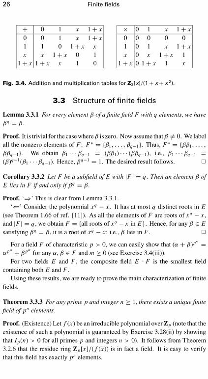
As 1 + x + x2 is irreducible over Z2, the ring Z2[x]/(1 + x + x2) is in facta field. This can also be verified by the addition and multiplication tables inFig. 3.4.

26 Finite fields

+ 0 1 x 1 + x0 0 1 x 1 + x1 1 0 1 + x xx x 1 + x 0 1

1 + x 1 + x x 1 0

× 0 1 x 1 + x0 0 0 0 01 0 1 x 1 + xx 0 x 1 + x 1

1 + x 0 1 + x 1 x

Fig. 3.4. Addition and multiplication tables for Z2[x]/(1 + x + x 2).

3.3 Structure of finite fields

Lemma 3.3.1 For every element β of a finite field F with q elements, we haveβq = β.

Proof. It is trivial for the case whereβ is zero. Now assume thatβ �= 0. We labelall the nonzero elements of F : F∗ = {β1, . . . , βq−1}. Thus, F∗ = {ββ1, . . . ,

ββq−1}. We obtain β1 · · · βq−1 = (ββ1) · · · (ββq−1), i.e., β1 · · · βq−1 =(β)q−1(β1 · · ·βq−1). Hence, βq−1 = 1. The desired result follows. �

Corollary 3.3.2 Let F be a subfield of E with |F | = q. Then an element β ofE lies in F if and only if βq = β.

Proof. ‘⇒’ This is clear from Lemma 3.3.1.‘⇐’ Consider the polynomial xq − x . It has at most q distinct roots in E

(see Theorem 1.66 of ref. [11]). As all the elements of F are roots of xq − x ,and |F | = q , we obtain F = {all roots of xq − x in E}. Hence, for any β ∈ Esatisfying βq = β, it is a root of xq − x ; i.e., β lies in F . �

For a field F of characteristic p > 0, we can easily show that (α + β)pm =α pm + β pm

for any α, β ∈ F and m ≥ 0 (see Exercise 3.4(iii)).For two fields E and F , the composite field E · F is the smallest field

containing both E and F .Using these results, we are ready to prove the main characterization of finite

fields.

Theorem 3.3.3 For any prime p and integer n ≥ 1, there exists a unique finitefield of pn elements.

Proof. (Existence) Let f (x) be an irreducible polynomial over Zp (note that theexistence of such a polynomial is guaranteed by Exercise 3.28(ii) by showingthat Ip(n) > 0 for all primes p and integers n > 0). It follows from Theorem3.2.6 that the residue ring Zp[x]/( f (x)) is in fact a field. It is easy to verifythat this field has exactly pn elements.

3.3 Structure of finite fields 27

(Uniqueness) Let E and F be two fields of pn elements. In the compositefield E · F , consider the polynomial x pn − x over E · F . By Corollary 3.3.2,E = {all roots of x pn − x} = F . �

From now on, it makes sense to denote the finite field with q elements byFq or G F(q).

For an irreducible polynomial f (x) of degree n over a field F , let α be a rootof f (x). Then the field F[x]/( f (x)) can be represented as

F[α] = {a0 + a1α + · · · + an−1αn−1 : ai ∈ F} (3.3)

if we replace x in F[x]/( f (x)) by α, as we did in Example 3.2.8(i). Anadvantage of using F[α] to replace the field F[x]/( f (x)) is that we can avoidthe confusion between an element of F[x]/( f (x)) and a polynomial over F .

Definition 3.3.4 An element α in a finite field Fq is called a primitive element(or generator) of Fq if Fq = {0, α, α2, . . . , αq−1}.

Example 3.3.5 Consider the field F4 = F2[α], where α is a root of the irre-ducible polynomial 1 + x + x2 ∈ F2[x]. Then we have

α2 = −(1+α) = 1+α, α3 = α(α2) = α(1+α) = α+α2 = α+1+α = 1.

Thus, F4 = {0, α, 1 + α, 1} = {0, α, α2, α3}, so α is a primitive element.

Definition 3.3.6 The order of a nonzero element α ∈ Fq , denoted by ord(α),is the smallest positive integer k such that αk = 1.

Example 3.3.7 Since there are no linear factors for the polynomial 1 + x2

over F3, 1 + x2 is irreducible over F3. Consider the element α in the fieldF9 = F3[α], where α is a root of 1 + x2. Then α2 = −1, α3 = α(α2) = −α

and

α4 = (α2)2 = (−1)2 = 1.

This means that ord(α) = 4.

Lemma 3.3.8 (i) The order ord(α) divides q − 1 for every α ∈ F∗q .

(ii) For two nonzero elements α, β ∈ F∗q , if gcd(ord(α), ord(β)) = 1, then

ord(αβ) = ord(α) × ord(β).

Proof. (i) Let m be a positive integer satisfying αm = 1. Write m = a ·ord(α)+b for some integers a ≥ 0 and 0 ≤ b < ord(α). Then

1 = αm = αa·ord(α)+b = (αord(α))a · αb = αb.

28 Finite fields

This forces b = 0; i.e., ord(α) is a divisor of m. Since αq−1 = 1, we obtainord(α)|(q − 1).

(ii) Put r = ord(α) × ord (β). It is clear that αr = 1 = βr as both ord(α)and ord(β) are divisors of r . Thus, (αβ)r = αrβr = 1. Therefore, ord(αβ) ≤ord (α) × ord(β). On the other hand, put t = ord(αβ). We have

1 = (αβ)t ·ord(α) = (αord(α))tβ t ·ord(α) = β t ·ord(α).

This implies that ord(β) divides t · ord(α) by the proof of part (i), so ord(β)divides t as ord(α) is prime to ord(β). In the same way, we can show that ord(α)divides t . This implies that ord(α) × ord(β) divides t . Thus, ord(αβ) = t ≥ord(α) × ord(β). The desired result follows. �

We now show the existence of primitive elements and give a characterizationof primitive elements in terms of their order.

Proposition 3.3.9 (i) A nonzero element of Fq is a primitive element if and onlyif its order is q − 1.

(ii) Every finite field has at least one primitive element.

Proof. (i) It is easy to see that α ∈ F∗q has order q − 1 if and only if the

elements α, α2, . . . , αq−1 are distinct. This is equivalent to saying that Fq ={0, α, α2, . . . , αq−1}.

(ii) Let m be the least common multiple of the orders of all the elements ofF∗

q . If rk is a prime power in the canonical factorization of m, then rk |ord(α)

for some α ∈ F∗q . The order of αord(α)/rk

is rk . Thus, if

m = rk11 · · · rkn

n

is the canonical factorization of m for distinct primes r1, . . . , rn , then for eachi = 1, . . . , n there exists βi ∈ F∗

q with ord(βi ) = rkii . Lemma 3.3.8(ii) implies

that there exists β ∈ F∗q with ord(β) = m. Now m|(q − 1) by Lemma 3.3.8(i),

and, on the other hand, all the q − 1 elements of F∗q are roots of the polynomial

xm − 1, so that m ≥ q − 1. Hence, ord(β) = m = q − 1, and the result followsfrom part (i). �

Remark 3.3.10 (i) Primitive elements are not unique. This can be seen fromExercises 3.12–3.15.

(ii) If α is a root of an irreducible polynomial of degree m over Fq , andit is also a primitive element of Fqm = Fq [α], then every element in Fqm canbe represented both as a polynomial in α and as a power of α, since Fqm ={a0 + a1α + · · · + am−1α

m−1 : ai ∈ Fq} = {0, α, α2, . . . , αqm−1}. Additionfor the elements of Fqm is easily carried out if the elements are represented

3.3 Structure of finite fields 29

Table 3.3. Elements of F8.

0 = 0 1 = α7 = α0 α = α1 α2 = α2

1 + α = α3 α + α2 = α4 1 + α + α2 = α5 1 + α2 = α6

as polynomials in α, whilst multiplication is easily done if the elements arerepresented as powers of α.

Example 3.3.11 Let α be a root of 1 + x + x3 ∈ F2[x] (by Example 3.2.2(iii),this polynomial is irreducible over F2). Hence, F8 = F2[α]. The order of α isa divisor of 8 − 1 = 7. Thus, ord(α) = 7 and α is a primitive element. In fact,any nonzero element in F8 except 1 is a primitive element. We list a table (seeTable 3.3) for the elements of F8 expressed in two forms.

Based on Table 3.3, both the addition and multiplication in F8 can be easilyimplemented. We use powers of α to represent the elements in F8. For instance,

α3 + α6 = (1 + α) + (1 + α2) = α + α2 = α4, α3 · α6 = α9 = α2.

From the above example, we know that both the addition and multiplication canbe carried out easily if we have a table representing the elements of finite fieldsboth in polynomial form and as powers of primitive elements. In fact, we cansimplify this table by using another table, called Zech’s log table, constructedas follows.

Let α be a primitive element of Fq . For each 0 ≤ i ≤ q − 2 or i = ∞, wedetermine and tabulate z(i) such that 1 + αi = αz(i) (note that we set α∞ = 0).Then for any two elements αi and α j with 0 ≤ i ≤ j ≤ q − 2 in Fq , we obtain

αi + α j = αi (1 + α j−i ) = αi+z( j−i) (mod q−1), αi · α j = αi+ j (mod q−1).

Example 3.3.12 Let α be a root of 1 + 2x + x3 ∈ F3[x]. This polynomial isirreducible over F3 as it has no linear factors. Hence, F27 = F3[α]. The orderof α is a divisor of 27 − 1 = 26. Thus, ord(α) is 2, 13 or 26. First, ord(α) �= 2;otherwise, α would be 1 or −1, neither of which is a root of 1 + 2x + x3.Furthermore, we have α13 = −1 �= 1. Thus, ord(α) = 26 and α is a primitiveelement of F27. After some computation, we obtain a Zech’s log table for F27

with respect to α (Table 3.4). Now we can carry out operations in F27 easily.For instance, we have

α7 + α11 = α7(1 + α4) = α7 · α18 = α25, α7 · α11 = α18.

30 Finite fields

Table 3.4. Zech’s log table for F27.

i z(i) i z(i) i z(i)

∞ 0 8 15 17 200 13 9 3 18 71 9 10 6 19 232 21 11 10 20 53 1 12 2 21 124 18 13 ∞ 22 145 17 14 16 23 246 11 15 25 24 197 4 16 22 25 8

3.4 Minimal polynomials

Let Fq be a subfield of Fr . For an element α of Fr , we are interested in nonzeropolynomials f (x) ∈ Fq [x] of the least degree such that f (α) = 0.

Definition 3.4.1 A minimal polynomial of an element α ∈ Fqm with respect toFq is a nonzero monic polynomial f (x) of the least degree in Fq [x] such thatf (α) = 0.

Example 3.4.2 Let α be a root of the polynomial 1 + x + x2 ∈ F2[x]. It isclear that the two linear polynomials x and 1 + x are not minimal polynomialsof α. Therefore, 1 + x + x2 is a minimal polynomial of α.

Since 1 + (1 + α) + (1 + α)2 = 1 + 1 + α + 1 + α2 = 1 + α + α2 = 0 and1 + α is not a root of x or 1 + x , 1 + x + x2 is also a minimal polynomial of1 + α.

Theorem 3.4.3 (i) The minimal polynomial of an element of Fqm with respectto Fq exists and is unique. It is also irreducible over Fq .

(ii) If a monic irreducible polynomial M(x) ∈ Fq [x] has α ∈ Fqm as a root,then it is the minimal polynomial of α with respect to Fq .

Proof. (i) Let α be an element of Fqm . As α is a root of xqm − x , we know theexistence of a minimal polynomial of α.

Suppose that M1(x), M2(x) ∈ Fq [x] are both minimal polynomials of α.By the division algorithm, we have M1(x) = s(x)M2(x) + r (x) for some

3.4 Minimal polynomials 31

polynomial r (x) with r (x) = 0 or deg(r (x)) < deg(M2(x)). Evaluating thepolynomials at α, we obtain 0 = M1(α) = s(α)M2(α) + r (α) = r (α). Bythe definition of minimal polynomials, this forces r (x) = 0; i.e., M2(x)|M1(x).Similarly, we have M1(x)|M2(x). Thus, we obtain M1(x) = M2(x) since bothare monic.

Let M(x) be the minimal polynomial of α. Suppose that it is reducible.Then we have two monic polynomials f (x) ∈ Fq [x] and g(x) ∈ Fq [x] suchthat deg( f (x)) < deg(M(x)), deg(g(x)) < deg(M(x)) and M(x) = f (x)g(x).Thus, we have 0 = M(α) = f (α)g(α), which implies that f (α) = 0 org(α) = 0. This contradicts the minimality of the degree of M(x).

(ii) Let f (x) be the minimal polynomial of α with respect to Fq . Bythe division algorithm, there exist polynomials h(x), e(x) ∈ Fq [x] such thatM(x) = h(x) f (x) + e(x) and deg(e(x)) < deg( f (x)). Evaluating the polyno-mials at α, we obtain 0 = M(α) = h(α) f (α) + e(α) = e(α). By the definitionof the minimal polynomial, this forces e(x) = 0. This implies that f (x) is thesame as M(x) since M(x) is a monic irreducible polynomial and f (x) cannotbe a nonzero constant. This completes the proof. �

Example 3.4.4 Let f (x) ∈ Fq [x] be a monic irreducible polynomial of degreem. Let α be a root of f (x). Then the minimal polynomial of α ∈ Fqm withrespect to Fq is f (x) itself. For instance, the minimal polynomial of a root of2 + x + x2 ∈ F3[x] is 2 + x + x2.

If we are given the minimal polynomial of a primitive element α ∈ Fqm , wewould like to find the minimal polynomial of αi , for any i . In order to do so,we have to start with cyclotomic cosets.

Definition 3.4.5 Let n be co-prime to q. The cyclotomic coset of q (or q-cyclotomic coset) modulo n containing i is defined by

Ci = {(i · q j (mod n)) ∈ Zn : j = 0, 1, . . .}.A subset {i1, . . . , it } of Zn is called a complete set of representatives of cyclo-tomic cosets of q modulo n if Ci1 , . . . , Cit are distinct and

⋃tj=1Ci j = Zn .

Remark 3.4.6 (i) It is easy to verify that two cyclotomic cosets are either equalor disjoint. Hence, the cyclotomic cosets partition Zn .

(ii) If n = qm − 1 for some m ≥ 1, each cyclotomic coset contains at mostm elements, as qm ≡ 1 (mod qm − 1).

(iii) It is easy to see that, in the case of n = qm −1 for some m ≥ 1, |Ci | = mif gcd(i, qm − 1) = 1.

32 Finite fields

Example 3.4.7 (i) Consider the cyclotomic cosets of 2 modulo 15:

C0 = {0}, C1 = {1, 2, 4, 8}, C3 = {3, 6, 9, 12},C5 = {5, 10}, C7 = {7, 11, 13, 14}.

Thus, C1 = C2 = C4 = C8, and so on. The set {0, 1, 3, 5, 7} is a complete setof representatives of cyclotomic cosets of 2 modulo 15. The set {0, 1, 6, 10, 7}is also a complete set of representatives of cyclotomic cosets of 2 modulo 15.

(ii) Consider the cyclotomic cosets of 3 modulo 26:

C0 = {0}, C1 = {1, 3, 9}, C2 = {2, 6, 18},C4 = {4, 12, 10}, C5 = {5, 15, 19}, C7 = {7, 21, 11},C8 = {8, 24, 20}, C13 = {13}, C14 = {14, 16, 22},C17 = {17, 25, 23}.

In this case, we have C1 = C3 = C9, and so on. The set {0, 1, 2, 4, 5, 7, 8,

13, 14, 17} is a complete set of representatives of cyclotomic cosets of 3modulo 26.

We are now ready to determine the minimal polynomials for all the elementsin a finite field.

Theorem 3.4.8 Let α be a primitive element of Fqm . Then the minimal poly-nomial of αi with respect to Fq is

M (i)(x) :=∏j∈Ci

(x − α j ),

where Ci is the unique cyclotomic coset of q modulo qm − 1 containing i .

Proof. Step 1: It is clear that αi is a root of M (i)(x) as i ∈ Ci .Step 2: Let M (i)(x) = a0 + a1x + · · · + ar xr , where ak ∈ Fqm and r = |Ci |.

Raising each coefficient to its qth power, we obtain

aq0 + aq

1 x + · · · + aqr xr =

∏j∈Ci

(x − αq j ) =∏j∈Cqi

(x − α j )

=∏j∈Ci

(x − α j ) = M (i)(x).

Note that we use the fact that Ci = Cqi in the above formula. Hence, ak = aqk

for all 0 ≤ k ≤ r ; i.e., ak are elements of Fq . This means that M (i)(x) is apolynomial over Fq .

Step 3: Since α is a primitive element, we have α j �= αk for two distinctelements j, k of Ci . Hence, M (i)(x) has no multiple roots. Now let f (x) ∈Fq [x] and f (αi ) = 0. Put

f (x) = f0 + f1x + · · · + fn xn

3.4 Minimal polynomials 33

for some fk ∈ Fq . Then, for any j ∈ Ci , there exists an integer l such thatj ≡ iql (mod qm − 1). Hence,

f (α j ) = f(αiql ) = f0 + f1α

iql + · · · + fnαniql

= f ql

0 + f ql

1 αiql + · · · + f ql

n αniql

= ( f0 + f1αi + · · · + fnα

ni )ql

= f (αi )ql = 0.

This implies that M (i)(x) is a divisor of f (x).The above three steps show that M (i)(x) is the minimal polynomial

of αi . �

Remark 3.4.9 (i) The degree of the minimal polynomial of αi is equal to thesize of the cyclotomic coset containing i .

(ii) From Theorem 3.4.8, we know that αi and αk have the same minimalpolynomial if and only if i, k are in the same cyclotomic coset.

Example 3.4.10 Let α be a root of 2 + x + x2 ∈ F3[x]; i.e.,

2 + α + α2 = 0. (3.4)

Then the minimal polynomial of α as well as α3 is 2 + x + x2. The minimalpolynomial of α2 is

M (2)(x) =∏j∈C2

(x − α j ) = (x − α2)(x − α6) = α8 − (α2 + α6)x + x2.

We know that α8 = 1 as α ∈ F9. To find M (2)(x), we have to simplify α2 + α6.We make use of the relationship (3.4) to obtain

α2 + α6 = (1 − α) + (1 − α)3 = 2 − α − α3

= 2 − α − α(1 − α) = 2 − 2α + α2 = 0.

Hence, the minimal polynomial of α2 is 1 + x2. In the same way, we mayobtain the minimal polynomial 2 + 2x + x2 of α5.

The following result will be useful when we study cyclic codes inChapter 7.

Theorem 3.4.11 Let n be a positive integer with gcd(q, n) = 1. Suppose thatm is a positive integer satisfying n|(qm − 1). Let α be a primitive elementof Fqm and let M ( j)(x) be the minimal polynomial of α j with respect to Fq .Let {s1, . . . , st } be a complete set of representatives of cyclotomic cosets of

34 Finite fields

q modulo n. Then the polynomial xn − 1 has the factorization into monicirreducible polynomials over Fq :

xn − 1 =t∏

i=1

M ((qm−1)si /n)(x).

Proof. Put r = (qm − 1)/n. Then αr is a primitive nth root of unity, and henceall the roots of xn − 1 are 1, αr , α2r , . . . , α(n−1)r . Thus, by the definition of theminimal polynomial, the polynomials M (ir )(x) are divisors of xn − 1, for all0 ≤ i ≤ n − 1. It is clear that we have

xn − 1 = lcm(M (0)(x), M (r )(x), M (2r )(x), . . . , M ((n−1)r )(x)).

In order to determine the factorization of xn − 1, it suffices to determine allthe distinct polynomials among M (0)(x), M (r )(x), M (2r )(x), . . . , M ((n−1)r )(x).By Remark 3.4.9, we know that M (ir )(x) = M ( jr )(x) if and only if ir andjr are in the same cyclotomic coset of q modulo qm − 1 = rn; i.e., i and jare in the same cyclotomic coset of q modulo n. This implies that all thedistinct polynomials among M (0)(x), M (r )(x), M (2r )(x), . . . , M ((n−1)r )(x) areM (s1r )(x), M (s2r )(x), . . . , M (st r )(x). The proof is completed. �

The following result follows immediately from the above theorem.

Corollary 3.4.12 Let n be a positive integer with gcd(q, n) = 1. Then thenumber of monic irreducible factors of xn − 1 over Fq is equal to the numberof cyclotomic cosets of q modulo n.

Example 3.4.13 (i) Consider the polynomial x13−1 over F3. It is easy to checkthat {0, 1, 2, 4, 7} is a complete set of representatives of cyclotomic cosets of3 modulo 13. Since 13 is a divisor of 33 − 1, we consider the field F27. Letα be a root of 1 + 2x + x3. By Example 3.3.12, α is a primitive element ofF27. By Example 3.4.7(ii), we know all the cyclotomic cosets of 3 modulo 26containing multiples of 2. Hence, we obtain

M (0)(x) = 2 + x,

M (2)(x) =∏j∈C2

(x − α j ) = (x − α2)(x − α6)(x − α18) = 2 + x + x2 + x3,

M (4)(x) =∏j∈C4

(x − α j ) = (x − α4)(x − α12)(x − α10) = 2 + x2 + x3,

M (8)(x) =∏j∈C8

(x − α j ) = (x − α8)(x − α20)(x − α24)

= 2 + 2x + 2x2 + x3,

3.4 Minimal polynomials 35

M (14)(x) =∏

j∈C14

(x − α j ) = (x − α14)(x − α16)(x − α22) = 2 + 2x + x3.

By Theorem 3.4.11, we obtain the factorization of x13 − 1 over F3 into monicirreducible polynomials:

x13 − 1 = M (0)(x)M (2)(x)M (4)(x)M (8)(x)M (14)(x)

= (2 + x)(2 + x + x2 + x3)(2 + x2 + x3)

× (2 + 2x + 2x2 + x3)(2 + 2x + x3).

(ii) Consider the polynomial x21 − 1 over F2. It is easy to check that{0, 1, 3, 5, 7, 9} is a complete set of representatives of cyclotomic cosets of2 modulo 21. Since 21 is a divisor of 26 − 1, we consider the field F64. Letα be a root of 1 + x + x6. It can be verified that α is a primitive element ofF64 (check that α3 �= 1, α7 �= 1, α9 �= 1 and α21 �= 1). We list the cyclotomiccosets of 2 modulo 63 containing multiples of 3:

C0 = {0}, C3 = {3, 6, 12, 24, 48, 33},C9 = {9, 18, 36}, C15 = {15, 30, 60, 57, 51, 39},C21 = {21, 42}, C27 = {27, 54, 45}.

Hence, we obtain

M (0)(x) = 1 + x,

M (3)(x) =∏j∈C3

(x − α j ) = 1 + x + x2 + x4 + x6,

M (9)(x) =∏j∈C9

(x − α j ) = 1 + x2 + x3,

M (15)(x) =∏

j∈C15

(x − α j ) = 1 + x2 + x4 + x5 + x6,

M (21)(x) =∏

j∈C21

(x − α j ) = 1 + x + x2,

M (27)(x) =∏

j∈C27

(x − α j ) = 1 + x + x3.

By Theorem 3.4.11, we obtain the factorization of x21 − 1 over F2 into monicirreducible polynomials:

x21 − 1 = M (0)(x)M (3)(x)M (9)(x)M (15)(x)M (21)(x)M (27)(x)

= (1 + x)(1 + x + x2 + x4 + x6)(1 + x2 + x3)

× (1 + x2 + x4 + x5 + x6)(1 + x + x2)(1 + x + x3).

36 Finite fields

Exercises

3.1 Show that the remainder of every square integer divided by 4 is either0 or 1. Hence, show that there do not exist integers x and y such thatx2 + y2 = 40 403.

3.2 Construct the addition and multiplication tables for the rings Z5 and Z8.3.3 Find the multiplicative inverse of each of the following elements:

(a) 2, 5 and 8 in Z11,(b) 4, 7 and 11 in Z17.

3.4 Let p be a prime.(i) Show that

(pj

) ≡ 0 (mod p) for any 1 ≤ j ≤ p − 1.

(ii) Show that(p−1

j

) ≡ (−1) j (mod p) for any 1 ≤ j ≤ p − 1.(iii) Show that, for any two elements α, β in a field of characteristic p,

we have

(α + β)pk = α pk + β pk

for any k ≥ 0.3.5 (i) Verify that f (x) = x5 − 1 ∈ F31[x] can be written as the product

(x2 − 3x + 2)(x3 + 3x2 + 7x + 15).(ii) Determine the remainder of f (x) divided by x2 − 3x + 2.

(iii) Compute the remainders of f (x) divided by x5, x7 and x4 + 5x3,respectively.

3.6 Verify that the following polynomials are irreducible:(a) 1 + x + x2 + x3 + x4, 1 + x + x4 and 1 + x3 + x4 over F2;(b) 1 + x2, 2 + x + x2 and 2 + 2x + x2 over F3.

3.7 Every quadratic or cubic polynomial is either irreducible or has a linearfactor.(a) Find the number of monic irreducible quadratic polynomials over Fq .(b) Find the number of monic irreducible cubic polynomials over Fq .(c) Determine all the irreducible quadratic and cubic polynomials over

F2.(d) Determine all the monic irreducible quadratic polynomials over F3.

3.8 Let f (x) = (2 + 2x2)(2 + x2 + x3)2(−1 + x4) ∈ F3[x] and g(x) =(1 + x2)(−2 + 2x2)(2 + x2 + x3) ∈ F3[x]. Determine gcd( f (x), g(x))and lcm( f (x), g(x)).

3.9 Find two polynomials u(x) and v(x) ∈ F2[x] such that deg(u(x)) < 4,deg(v(x)) < 3 and

u(x)(1 + x + x3) + v(x)(1 + x + x2 + x3 + x4) = 1.

Exercises 37

3.10 Construct both the addition and multiplication tables for the ringF3[x]/(x2 + 2).

3.11 (a) Find the order of the elements 2, 7, 10 and 12 in F17.(b) Find the order of the elements α, α3, α + 1 and α3 + 1 in F16, where

α is a root of 1 + x + x4.3.12 (i) Let α be a primitive element of Fq . Show that αi is also a primitive

element if and only if gcd(i, q − 1) = 1.(ii) Determine the number of primitive elements in the following fields:

F9, F19, F25 and F32.3.13 Determine all the primitive elements of the following fields: F7, F8 and F9.

3.14 Show that all the nonzero elements, except the identity 1, in F128 areprimitive elements.

3.15 Show that any root of 1 + x + x6 ∈ F2[x] is a primitive element of F64.3.16 Consider the field with 16 elements constructed using the irreducible

polynomial f (x) = 1 + x3 + x4 over F2.(i) Let α be a root of f (x). Show that α is a primitive element of F16.

Represent each element both as a polynomial and as a power of α.(ii) Construct a Zech’s log table for the field.

3.17 Find a primitive element and construct a Zech’s log table for each of thefollowing finite fields:(a) F32 , (b) F25 , (c) F52 .

3.18 Show that each monic irreducible polynomial of Fq [x] of degree m is theminimal polynomial of some element of Fqm with respect to Fq .

3.19 Let α be a root of 1 + x3 + x4 ∈ F2[x].(i) List all the cyclotomic cosets of 2 modulo 15.

(ii) Find the minimal polynomial of αi ∈ F16, for all 1 ≤ i ≤ 14.(iii) Using Exercise 3.18, find all the irreducible polynomials of degree

4 over F2.3.20 (i) Find all the cyclotomic cosets of 2 modulo 31.

(ii) Find the minimal polynomials of α, α4 and α5, where α is a root of1 + x2 + x5 ∈ F2[x].

3.21 Based on the cyclotomic cosets of 3 modulo 26, find all the monic irre-ducible polynomials of degree 3 over F3.

3.22 (i) Prove that, if k is a positive divisor of m, then Fpm contains a uniquesubfield with pk elements.

(ii) Determine all the subfields in (a) F212 , (b) F218 .3.23 Factorize the following polynomials:

(a) x7 − 1 over F2; (b) x15 − 1 over F2;(c) x31 − 1 over F2; (d) x8 − 1 over F3;(e) x12 − 1 over F5; (f) x24 − 1 over F7.

38 Finite fields

3.24 Show that, for any given element c of Fq , there exist two elements a andb of Fq such that a2 + b2 = c.

3.25 For a nonzero element b of Fp, where p is a prime, prove that the trinomialx p − x − b is irreducible in Fpn [x] if and only if n is not divisible by p.

3.26 (Lagrange interpolation formula.) For n ≥ 1, let α1, . . . , αn be n distinctelements of Fq , and let β1, . . . , βn be n arbitrary elements of Fq . Showthat there exists exactly one polynomial f (x) ∈ Fq [x] of degree ≤ n − 1such that f (αi ) = βi for i = 1, . . . , n. Furthermore, show that thispolynomial is given by

f (x) =n∑

i=1

βi

g′(αi )

n∏k=1k �=i

(x − αk),

where g′(x) denotes the derivative of g(x) := ∏nk=1(x − αk).

3.27 (i) Show that, for every integer n ≥ 1, the product of all monicirreducible polynomials over Fq whose degrees divide n is equalto xqn − x .

(ii) Let Iq (d) denote the number of monic irreducible polynomials ofdegree d in Fq [x]. Show that

qn =∑d|n

d Iq (d) for all n ∈ N,

where the sum is extended over all positive divisors d of n.3.28 The Mobius function on the set N of positive integers is defined by

µ(n) =

1 if n = 1(−1)k if n is a product of k distinct primes0 if n is divisible by the square of a prime.

(i) Let h and H be two functions from N to Z. Show that

H (n) =∑d|n

h(d)

for all n ∈ N if and only if

h(n) =∑d|n

µ(d)H(n

d

)

for all n ∈ N.(ii) Show that the number Iq (n) of monic irreducible polynomials over

Fq of degree n is given by

Iq (n) = 1

n

∑d|n

µ(d)qn/d .

4 Linear codes

A linear code of length n over the finite field Fq is simply a subspace of thevector space Fn

q . Since linear codes are vector spaces, their algebraic structuresoften make them easier to describe and use than nonlinear codes. In most ofthis book, we focus our attention on linear codes over finite fields.

4.1 Vector spaces over finite fields

We recall some definitions and facts about vector spaces over finite fields. Whilethe proofs of most of the facts stated in this section are omitted, it should benoted that many of them are practically identical to those in the case of vectorspaces over R or C.

Definition 4.1.1 Let Fq be the finite field of order q. A nonempty set V ,together with some (vector) addition + and scalar multiplication by elementsof Fq , is a vector space (or linear space) over Fq if it satisfies all of the followingconditions. For all u, v, w ∈ V and for all λ, µ ∈ Fq :

(i) u + v ∈ V ;(ii) (u + v) + w = u + (v + w);

(iii) there is an element 0 ∈ V with the property 0 + v = v = v + 0 for allv ∈ V ;

(iv) for each u ∈ V there is an element of V , called −u, such that u+ (−u) =0 = (−u) + u;

(v) u + v = v + u;(vi) λv ∈ V ;

(vii) λ(u + v) = λu + λv, (λ + µ)u = λu + µu;(viii) (λµ)u = λ(µu);

(ix) if 1 is the multiplicative identity of Fq , then 1u = u.

39

40 Linear codes

Let Fnq be the set of all vectors of length n with entries in Fq :

Fnq = {(v1, v2, . . . , vn) : vi ∈ Fq}.

We define the vector addition for Fnq componentwise, using the addition defined

on Fq ; i.e., if

v = (v1, . . . , vn) ∈ Fnq and w = (w1, . . . , wn) ∈ Fn

q ,

then

v + w = (v1 + w1, . . . , vn + wn) ∈ Fnq .

We also define the scalar multiplication for Fnq componentwise; i.e., if

v = (v1, . . . , vn) ∈ Fnq and λ ∈ Fq ,

then

λv = (λv1, . . . , λvn) ∈ Fnq .

Let 0 denote the zero vector (0, 0, . . . , 0) ∈ Fnq .

Example 4.1.2 It is easy to verify that the following are vector spaces over Fq :

(i) (any q) C1 = Fnq and C2 = {0};

(ii) (any q) C3 = {(λ, . . . , λ) : λ ∈ Fq};(iii) (q = 2) C4 = {(0, 0, 0, 0), (1, 0, 1, 0), (0, 1, 0, 1), (1, 1, 1, 1)};(iv) (q = 3) C5 = {(0, 0, 0), (0, 1, 2), (0, 2, 1)}.

Remark 4.1.3 When no confusion arises, it is sometimes convenient to writea vector (v1, v2, . . . , vn) simply as v1v2 · · · vn .

Definition 4.1.4 A nonempty subset C of a vector space V is a subspace of V ifit is itself a vector space with the same vector addition and scalar multiplicationas V .

Example 4.1.5 Using the same notation as in Example 4.1.2, it is easy to seethat:

(i) (any q) C2 = {0} is a subspace of both C3 and C1 = Fnq , and C3 is a

subspace of C1 = Fnq ;

(ii) (q = 2) C4 is a subspace of F42;

(iii) (q = 3) C5 is a subspace of F33.

4.1 Vector spaces over finite fields 41

Proposition 4.1.6 A nonempty subset C of a vector space V over Fq is asubspace if and only if the following condition is satisfied:

if x, y ∈ C and λ, µ ∈ Fq , then λx + µy ∈ C.

We leave the proof of Proposition 4.1.6 as an exercise (see Exercise 4.1).Note that, when q = 2, a necessary and sufficient condition for a nonemptysubset C of a vector space V over F2 to be a subspace is: if x, y ∈ C , thenx + y ∈ C .

Definition 4.1.7 Let V be a vector space over Fq . A linear combination ofv1, . . . , vr ∈ V is a vector of the form λ1v1 +· · ·+λr vr , where λ1, . . . , λr ∈ Fq

are some scalars.

Definition 4.1.8 Let V be a vector space over Fq . A set of vectors {v1, . . . , vr }in V is linearly independent if

λ1v1 + · · · + λr vr = 0 ⇒ λ1 = · · · = λr = 0.

The set is linearly dependent if it is not linearly independent; i.e., if there areλ1, . . . , λr ∈ Fq , not all zero (but maybe some are!), such that λ1v1 + · · · +λr vr = 0.

Example 4.1.9 (i) Any set S which contains 0 is linearly dependent.(ii) For any Fq , {(0, 0, 0, 1), (0, 0, 1, 0), (0, 1, 0, 0)} is linearly independent.(iii) For any Fq , {(0, 0, 0, 1), (1, 0, 0, 0), (1, 0, 0, 1)} is linearly dependent.

Definition 4.1.10 Let V be a vector space over Fq and let S = {v1, v2, . . . , vk}be a nonempty subset of V . The (linear) span of S is defined as

< S >= {λ1v1 + · · · + λkvk : λi ∈ Fq}.If S = ∅, we define < S >= {0}. It is easy to verify that < S > is a subspace ofV , called the subspace generated (or spanned) by S. Given a subspace C of V ,a subset S of C is called a generating set (or spanning set) of C if C =< S >.

Remark 4.1.11 If S is already a subspace of V , then < S >= S.

Example 4.1.12 (i) If q = 2 and S = {0001, 0010, 0100}, then

< S >= {0000, 0001, 0010, 0100, 0011, 0101, 0110, 0111}.(ii) If q = 2 and S = {0001, 1000, 1001}, then

< S >= {0000, 0001, 1000, 1001}.

42 Linear codes

(iii) If q = 3 and S = {0001, 1000, 1001}, then

< S >= {0000, 0001, 0002, 1000, 2000, 1001, 1002, 2001, 2002}.

Definition 4.1.13 Let V be a vector space over Fq . A nonempty subset B ={v1, v2, . . . , vk} of V is called a basis for V if V = < B > and B is linearlyindependent.

Remark 4.1.14 (i) If B = {v1, . . . , vk} is a basis of V , then any vector v ∈ Vcan be expressed as a unique linear combination of vectors in B; i.e., there existunique λ1, λ2, . . . , λk ∈ Fq such that

v = λ1v1 + λ2v2 + · · · + λkvk .

(ii) A vector space V over a finite field Fq can have many bases; but all basescontain the same number of elements. This number is called the dimension ofV over Fq , denoted by dim(V ). In the case where V can be regarded as a vectorspace over more than one field, the notation dimFq (V ) may be used to avoidconfusion.

Theorem 4.1.15 Let V be a vector space over Fq . If dim(V ) = k, then

(i) V has qk elements;(ii) V has 1

k!

∏k−1i=0

(qk − qi

)different bases.

Proof. (i) If {v1, . . . , vk} is a basis for V , then

V = {λ1v1 + · · · + λkvk : λ1, . . . , λk ∈ Fq}.

Since |Fq | = q , there are exactly q choices for each of λ1, . . . , λk ; hence, Vhas exactly qk elements.

(ii) Let B = {v1, . . . , vk} denote a basis for V . Since v1 �= 0, there areqk − 1 choices for v1. For B to be a basis, the condition v2 �∈<v1 > is needed,so there are qk − q choices for v2. Arguing in this manner, for every i suchthat k ≥ i ≥ 2, we need vi �∈<v1, . . . , vi−1 >, so there are qk − qi−1 choicesfor vi . Hence, there are

∏k−1i=0 (qk − qi ) distinct ordered k-tuples (v1, . . . , vk).

However, since the order of v1, . . . , vk is irrelevant for a basis, the number ofdistinct bases for V is 1

k!

∏k−1i=0

(qk − qi

). �

4.1 Vector spaces over finite fields 43

Example 4.1.16 Let q = 2, S = {0001, 0010, 0100} and V =< S >, then

V = {0000, 0001, 0010, 0100, 0011, 0101, 0110, 0111}.

Note that S is linearly independent, so dim(V ) = 3. We see that |V | = 8 = 23.By Theorem 4.1.15, the number of different bases for V is given by

1

k!

k−1∏i=0

(2k − 2i ) = 1

3!(23 − 1)(23 − 2)(23 − 22) = 28.

Definition 4.1.17 Let v = (v1, v2, . . . , vn), w = (w1, w2, . . . , wn) ∈ Fnq .

(i) The scalar product (also known as the dot product or the Euclidean innerproduct) of v and w is defined as

v · w = v1w1 + · · · + vnwn ∈ Fq .

(ii) The two vectors v and w are said to be orthogonal if v · w = 0.(iii) Let S be a nonempty subset of Fn

q . The orthogonal complement S⊥ ofS is defined to be

S⊥ = {v ∈ Fnq : v · s = 0 for all s ∈ S}.

If S = ∅, then we define S⊥ = Fnq .

Remark 4.1.18 (i) It is easy to verify that S⊥ is always a subspace of the vectorspace Fn

q for any subset S of Fnq , and that < S >⊥= S⊥.

(ii) The scalar product is an example of an inner product on Fnq . An inner

product on Fnq is a pairing 〈, 〉 : Fn

q × Fnq → Fq satisfying the following

conditions: for all u, v, w ∈ Fnq ,

(a) 〈u + v, w〉 = 〈u, w〉 + 〈v, w〉;(b) 〈u, v + w〉 = 〈u, v〉 + 〈u, w〉;(c) 〈u, v〉 = 0 for all u ∈ Fn

q if and only if v = 0;(d) 〈u, v〉 = 0 for all v ∈ Fn

q if and only if u = 0.

The scalar product in Definition 4.1.17 is often called the Euclidean innerproduct. Some other inner products, such as the Hermitian inner product andsymplectic inner product, are also used in coding theory (see Exercises 4.9–4.13). Throughout this book, unless it is otherwise specified, the inner prod-uct used is always assumed to be the scalar product, i.e., the Euclidean innerproduct.

44 Linear codes

Example 4.1.19 (i) Let q = 2 and let n = 4. If u = (1, 1, 1, 1), v =(1, 1, 1, 0), w = (1, 0, 0, 1), then

u · v = 1 · 1 + 1 · 1 + 1 · 1 + 1 · 0 = 1,

u · w = 1 · 1 + 1 · 0 + 1 · 0 + 1 · 1 = 0,

v · w = 1 · 1 + 1 · 0 + 1 · 0 + 0 · 1 = 1.

Hence, u and w are orthogonal.(ii) Let q = 2 and let S = {0100, 0101}. To find S⊥, let v = (v1, v2, v3, v4) ∈

S⊥. Then

v · (0, 1, 0, 0) = 0 ⇒ v2 = 0,

v · (0, 1, 0, 1) = 0 ⇒ v2 + v4 = 0.

Hence, we have v2 = v4 = 0. Since v1 and v3 can be either 0 or 1, we canconclude that

S⊥ = {0000, 0010, 1000, 1010}.

Theorem 4.1.20 Let S be a subset of Fnq , then we have

dim(< S >) + dim(S⊥) = n.

Proof. Theorem 4.1.20 is obviously true when < S >= {0}.Now let dim(< S >) = k ≥ 1 and suppose {v1, . . . , vk} is a basis of < S >.

We need to show that dim(S⊥) = dim(< S >⊥) = n − k.Note that x ∈ S⊥ if and only if

v1 · x = · · · = vk · x = 0,

which is equivalent to saying that x satisfies AxT = 0, where A is the k × nmatrix whose i th row is vi .

The rows of A are linearly independent, so AxT = 0 is a linear system of klinearly independent equations in n variables. From linear algebra, it is knownthat such a system admits a solution space of dimension n − k. �

Example 4.1.21 Let q = 2, n = 4 and S = {0100, 0101}. Then

< S > = {0000, 0100, 0001, 0101}.Note that S is linearly independent, so dim(< S >) = 2. We have computedthat (Example 4.1.19)

S⊥ = {0000, 0010, 1000, 1010}.

4.2 Linear codes 45

Note that {0010, 1000} is a basis for S⊥, so dim(S⊥) = 2. Hence, we haveverified that

dim(< S >) + dim(S⊥) = 2 + 2 = 4 = n.

4.2 Linear codes

We are now ready to introduce linear codes and discuss some of their elementaryproperties.

Definition 4.2.1 A linear code C of length n over Fq is a subspace of Fnq .

Example 4.2.2 The following are linear codes:

(i) C = {(λ, λ, . . . , λ) : λ ∈ Fq}. This code is often called a repetition code(refer also to Example 1.0.3).

(ii) (q = 2) C = {000, 001, 010, 011}.(iii) (q = 3) C = {0000, 1100, 2200, 0001, 0002, 1101, 1102, 2201, 2202}.(iv) (q = 2) C = {000, 001, 010, 011, 100, 101, 110, 111}.

Definition 4.2.3 Let C be a linear code in Fnq .

(i) The dual code of C is C⊥, the orthogonal complement of the subspace Cof Fn

q .(ii) The dimension of the linear code C is the dimension of C as a vector

space over Fq , i.e., dim(C).

Theorem 4.2.4 Let C be a linear code of length n over Fq . Then,

(i) |C | = qdim(C), i.e., dim(C) = logq |C |;(ii) C⊥ is a linear code and dim(C) + dim(C⊥) = n;

(iii) (C⊥)⊥ = C.

Proof. (i) follows from Theorem 4.1.15(i).(ii) follows immediately from Remark 4.1.18(i) and Theorem 4.1.20 with

C = S.Using the equality in (ii) and a similar equality with C replaced by C⊥, we

obtain dim(C) = dim((C⊥)⊥). To prove (iii), it therefore suffices to show thatC ⊆ (C⊥)⊥.

Let c ∈ C . To show that c ∈ (C⊥)⊥, we need to show that c · x = 0 forall x ∈ C⊥. Since c ∈ C and x ∈ C⊥, by the definition of C⊥, it follows thatc · x = 0. Hence, (iii) is proved. �

46 Linear codes

Example 4.2.5 (i) (q = 2) Let C = {0000, 1010, 0101, 1111}, so dim(C) =log2 |C | = log2 4 = 2. It is easy to see that C⊥ = {0000, 1010, 0101, 1111} =C , so dim(C⊥) = 2. In particular, Theorem 4.2.4(ii) and (iii) are verified.

(ii) (q = 3) Let C = {000, 001, 002, 010, 020, 011, 012, 021, 022}, sodim(C) = log3 |C | = log3 9 = 2. One checks readily that C⊥ = {000, 100,

200}, so dim(C⊥) = 1.

Remark 4.2.6 A linear code C of length n and dimension k over Fq is oftencalled a q-ary [n, k]-code or, if q is clear from the context, an [n, k]-code. It isalso an (n, qk)-linear code. If the distance d of C is known, it is also sometimesreferred to as an [n, k, d]-linear code.

Definition 4.2.7 Let C be a linear code.(i) C is self-orthogonal if C ⊆ C⊥.(ii) C is self-dual if C = C⊥.

Proposition 4.2.8 The dimension of a self-orthogonal code of length n mustbe ≤n/2, and the dimension of a self-dual code of length n is n/2.

Proof. This proposition is an immediate consequence of Theorem 4.2.4(ii) andthe definitions of self-orthogonal and self-dual codes. �

Example 4.2.9 The code in Example 4.2.5(i) is self-dual.

4.3 Hamming weight

Recall that the Hamming distance d(x, y) between two words x, y ∈ Fnq was

defined in Chapter 2.

Definition 4.3.1 Let x be a word in Fnq . The (Hamming) weight of x, denoted

by wt(x), is defined to be the number of nonzero coordinates in x; i.e.,

wt(x) = d(x, 0),

where 0 is the zero word.

Remark 4.3.2 For every element x of Fq , we can define the Hamming weightas follows:

wt(x) = d(x, 0) ={

1 if x �= 00 if x = 0.

4.3 Hamming weight 47

Table 4.1.

x y x � y wt(x) + wt(y) − 2wt(x � y) wt(x + y)

0 0 0 0 00 1 0 1 11 0 0 1 11 1 1 0 0

Then, writing x ∈ Fnq as x = (x1, x2, . . . , xn), the Hamming weight of x can

also be equivalently defined as

wt(x) = wt(x1) + wt(x2) + · · · + wt(xn). (4.1)

Lemma 4.3.3 If x, y ∈ Fnq , then d(x, y) = wt(x − y).

Proof. For x, y ∈ Fq , d(x, y) = 0 if and only if x = y, which is true if andonly if x − y = 0 or, equivalently, wt(x − y) = 0. Lemma 4.3.3 now followsfrom (2.1) and (4.1). �

Since a = −a for all a ∈ Fq when q is even, the following corollary is animmediate consequence of Lemma 4.3.3.

Corollary 4.3.4 Let q be even. If x, y ∈ Fnq , then d(x, y) = wt(x + y).

For x = (x1, x2, . . . , xn) and y = (y1, y2, . . . , yn) in Fnq , let

x � y = (x1 y1, x2 y2, . . . , xn yn).

Lemma 4.3.5 If x, y ∈ Fn2 , then

wt(x + y) = wt(x) + wt(y) − 2wt(x � y). (4.2)

Proof. From (4.1), it is enough to show that (4.2) is true for x, y ∈ F2. Thiscan be easily verified as in Table 4.1. �

Clearly, Lemma 4.3.5 implies that wt(x) + wt(y) ≥ wt(x + y) for x, y ∈ Fn2.

In fact, this inequality is true for any alphabet Fq . The proof of the followinglemma is left as an exercise (see Exercise 4.18).

Lemma 4.3.6 For any prime power q and x, y ∈ Fnq , we have

wt(x) + wt(y) ≥ wt(x + y) ≥ wt(x) − wt(y). (4.3)

48 Linear codes

Definition 4.3.7 Let C be a code (not necessarily linear). The minimum(Hamming) weight of C , denoted wt(C), is the smallest of the weights of thenonzero codewords of C .

Theorem 4.3.8 Let C be a linear code over Fq . Then d(C) = wt(C).

Proof. Recall that for any words x, y we have d(x, y) = wt(x − y).By definition, there exist x′, y′ ∈ C such that d(x′, y′) = d(C), so

d(C) = d(x′, y′) = wt(x′ − y′) ≥ wt(C),

since x′ − y′ ∈ C .Conversely, there is a z ∈ C\{0} such that wt(C) = wt(z), so

wt(C) = wt(z) = d(z, 0) ≥ d(C). �

Example 4.3.9 Consider the binary linear code C = {0000, 1000, 0100,

1100}. We see that

wt(1000) = 1,

wt(0100) = 1,

wt(1100) = 2.

Hence, d(C) = 1.

Remark 4.3.10 (Some advantages of linear codes.) The following are someof the reasons why it may be preferable to use linear codes over nonlinear ones:

(i) As a linear code is a vector space, it can be described completely by usinga basis (see Section 4.4).

(ii) The distance of a linear code is equal to the smallest weight of its nonzerocodewords.

(iii) The encoding and decoding procedures for a linear code are faster andsimpler than those for arbitrary nonlinear codes (see Sections 4.7 and 4.8).

4.4 Bases for linear codes

Since a linear code is a vector space, all its elements can be described in termsof a basis. In this section, we discuss three algorithms that yield either a basisfor a given linear code or its dual. We first recall some facts from linear algebra.

4.4 Bases for linear codes 49

Definition 4.4.1 Let A be a matrix over Fq ; an elementary row operationperformed on A is any one of the following three operations:

(i) interchanging two rows,(ii) multiplying a row by a nonzero scalar,

(iii) replacing a row by its sum with the scalar multiple of another row.

Definition 4.4.2 Two matrices are row equivalent if one can be obtained fromthe other by a sequence of elementary row operations.

The following are well known facts from linear algebra:

(i) Any matrix M over Fq can be put in row echelon form (REF ) or reducedrow echelon form (RREF ) by a sequence of elementary row operations. Inother words, a matrix is row equivalent to a matrix in REF or in RREF.

(ii) For a given matrix, its RREF is unique, but it may have different REFs.(Recall that the difference between the RREF and the REF is that theleading nonzero entry of a row in the RREF is equal to 1 and it is the onlynonzero entry in its column.)

We are now ready to describe the three algorithms.

Algorithm 4.1

Input: A nonempty subset S of Fnq .

Output: A basis for C = < S >, the linear code generated by S.

Description: Form the matrix A whose rows are the words in S. Useelementary row operations to find an REF of A. Then the nonzerorows of the REF form a basis for C .

Example 4.4.3 Let q = 3. Find a basis for C = < S >, where

S = {12101, 20110, 01122, 11010}.

A =

12101201100112211010

→

12101022110112202212

→

12101011220000100000

.

The last matrix is in REF. By Algorithm 4.1, {12101, 01122, 00001} is a basisfor C .

50 Linear codes

Algorithm 4.2

Input: A nonempty subset S of Fnq .

Output: A basis for C = < S >, the linear code generated by S.

Description: Form the matrix A whose columns are the words in S.Use elementary row operations to put A in REF and locate the leadingcolumns in the REF. Then the original columns of A corresponding tothese leading columns form a basis for C .

Example 4.4.4 Let q = 2. Find a basis for C = < S >, where

S = {11101, 10110, 01011, 11010}.

A =

11011011110001111010

→

11010110000101110111

→

11010110000100000000

.

Since columns 1, 2 and 4 of the REF are the leading columns, Algorithm 4.2says that columns 1, 2 and 4 of A form a basis for C ; i.e., {11101, 10110, 11010}is a basis for C .

Remark 4.4.5 Note that the basis that Algorithm 4.2 yields is a subset of thegiven set S, while this is not necessarily the case for Algorithm 4.1.

Algorithm 4.3

Input: A nonempty subset S of Fnq .

Output: A basis for the dual code C⊥, where C = < S >.

Description: Form the matrix A whose rows are the words in S. Useelementary row operations to place A in RREF. Let G be the k × nmatrix consisting of all the nonzero rows of the RREF:

A →(

GO

).

(Here, O denotes the zero matrix.)The matrix G contains k leading columns. Permute the columns of

G to form

G ′ = (Ik |X ) ,

4.4 Bases for linear codes 51

where Ik denotes the k × k identity matrix. Form a matrix H ′ asfollows:

H ′ = (−XT|In−k),

where XT denotes the transpose of X .Apply the inverse of the permutation applied to the columns of G

to the columns of H ′ to form H . Then the rows of H form a basis forC⊥.

Remark 4.4.6 (i) Notice that Algorithm 4.3 also provides a basis for C sinceit includes Algorithm 4.1.

(ii) An explanation of the principles behind Algorithm 4.3 is given in The-orem 4.5.9 in the following section.

Example 4.4.7 Let q = 3. Find a basis for C⊥ if the RREF of A is

G =

1 2 3 4 5 6 7 8 9 10

1 0 2 0 0 2 0 1 0 20 0 0 1 0 1 0 0 0 10 0 0 0 1 0 0 2 0 00 0 0 0 0 0 1 0 0 10 0 0 0 0 0 0 0 1 2

.

The leading columns of G are columns 1, 4, 5, 7 and 9. We permute the columnsof G into the order 1, 4, 5, 7, 9, 2, 3, 6, 8, 10 to form the matrix

G ′ = (I5|X ) =

1 4 5 7 9 2 3 6 8 10

1 0 0 0 0 0 2 2 1 20 1 0 0 0 0 0 1 0 10 0 1 0 0 0 0 0 2 00 0 0 1 0 0 0 0 0 10 0 0 0 1 0 0 0 0 2

.

Form the matrix H ′ and finally rearrange the columns of H ′ using the inversepermutation to obtain H :

H ′ =

1 4 5 7 9 2 3 6 8 10

0 0 0 0 0 1 0 0 0 01 0 0 0 0 0 1 0 0 01 2 0 0 0 0 0 1 0 02 0 1 0 0 0 0 0 1 01 2 0 2 1 0 0 0 0 1

,

52 Linear codes

H =

1 2 3 4 5 6 7 8 9 10

0 1 0 0 0 0 0 0 0 01 0 1 0 0 0 0 0 0 01 0 0 2 0 1 0 0 0 02 0 0 0 1 0 0 1 0 01 0 0 2 0 0 2 0 1 1

.

By Algorithm 4.3, the rows of H form a basis for C⊥.

4.5 Generator matrix and parity-check matrix

Knowing a basis for a linear code enables us to describe its codewords explicitly.In coding theory, a basis for a linear code is often represented in the form ofa matrix, called a generator matrix, while a matrix that represents a basis forthe dual code is called a parity-check matrix. These matrices play an importantrole in coding theory.

Definition 4.5.1 (i) A generator matrix for a linear code C is a matrix G whoserows form a basis for C .

(ii) A parity-check matrix H for a linear code C is a generator matrix for thedual code C⊥.

Remark 4.5.2 (i) If C is an [n, k]-linear code, then a generator matrix for Cmust be a k × n matrix and a parity-check matrix for C must be an (n − k) × nmatrix.

(ii) Algorithm 4.3 of Section 4.4 can be used to find generator and parity-check matrices for a linear code.

(iii) As the number of bases for a vector space usually exceeds one, the num-ber of generator matrices for a linear code also usually exceeds one. Moreover,even when the basis is fixed, a permutation (different from the identity) of therows of a generator matrix also leads to a different generator matrix.

(iv) The rows of a generator matrix are linearly independent. The sameholds for the rows of a parity-check matrix. To show that a k × n matrix G isindeed a generator matrix for a given [n, k]-linear code C , it suffices to showthat the rows of G are codewords in C and that they are linearly independent.Alternatively, one may also show that C is contained in the row space of G.

Definition 4.5.3 (i) A generator matrix of the form (Ik |X ) is said to be instandard form.

(ii) A parity-check matrix in the form (Y |In−k) is said to be in standard form.

4.5 Generator matrix and parity-check matrix 53

Lemma 4.5.4 Let C be an [n, k]-linear code over Fq , with generator matrixG. Then v ∈ Fn

q belongs to C⊥ if and only if v is orthogonal to every row ofG; i.e., v ∈ C⊥ ⇔ vGT = 0. In particular, given an (n − k) × n matrix H,then H is a parity-check matrix for C if and only if the rows of H are linearlyindependent and H GT = O.

Proof. Let ri denote the i th row of G. In particular, ri ∈ C for all 1 ≤ i ≤ k,and every c ∈ C may be written as

c = λ1r1 + · · · + λkrk,

where λ1, . . . , λk ∈ Fq .If v ∈ C⊥, then v · c = 0 for all c ∈ C . In particular, v is orthogonal to ri ,

for all 1 ≤ i ≤ k; i.e., vGT = 0.Conversely, if v · ri = 0 for all 1 ≤ i ≤ k, then clearly, for any c =

λ1r1 + · · · + λkrk ∈ C ,

v · c = λ1(v · r1) + · · · + λk(v · rk) = 0.

For the last statement, if H is a parity-check matrix for C , then the rows ofH are linearly independent by definition. Since the rows of H are codewordsin C⊥, it follows from the earlier statement that H GT = O .

Conversely, if H GT = O , then the earlier statement shows that the rowsof H , and hence the row space of H , are contained in C⊥. Since the rowsof H are linearly independent, the row space of H has dimension n − k, sothe row space of H is indeed C⊥. In other words, H is a parity-check matrixfor C . �

Remark 4.5.5 An alternative but equivalent formulation for Lemma 4.5.4 isthe following:

Let C be an [n, k]-linear code over Fq , with parity-check matrix H. Thenv ∈ Fn

q belongs to C if and only if v is orthogonal to every row of H; i.e.,v ∈ C ⇔ vH T = 0. In particular, given a k × n matrix G, then G is agenerator matrix for C if and only if the rows of G are linearly independentand G H T = O.

One of the consequences of Lemma 4.5.4 is the following theorem relatingthe distance d of a linear code C to properties of a parity-check matrix of C .When d is small, Corollary 4.5.7 can be a useful way to determine d.

Theorem 4.5.6 Let C be a linear code and let H be a parity-check matrix forC. Then

54 Linear codes

(i) C has distance ≥ d if and only if any d − 1 columns of H are linearlyindependent; and

(ii) C has distance ≤ d if and only if H has d columns that are linearlydependent.

Proof. Let v = (v1, . . . , vn) ∈ C be a word of weight e > 0. Supposethe nonzero coordinates are in the positions i1, . . . , ie, so that v j = 0 if j �∈{i1, . . . , ie}. Let ci (1 ≤ i ≤ n) denote the i th column of H .

By Lemma 4.5.4 (or, more precisely, its equivalent formulation inRemark 4.5.5), C contains a nonzero word v = (v1, . . . , vn) of weight e (whosenonzero coordinates are vi1 , . . . , vie ) if and only if

0 = vH T = vi1 cTi1

+ · · · + vie cTie,

which is true if and only if there are e columns of H (namely, ci1 , . . . , cie ) thatare linearly dependent.

To say that the distance of C is ≥ d is equivalent to saying that C does notcontain any nonzero word of weight ≤ d − 1, which is in turn equivalent tosaying that any ≤ d −1 columns of H are linearly independent. This proves (i).

Similarly, to say that the distance of C is ≤ d is equivalent to saying that Ccontains a nonzero word of weight ≤ d, which is in turn equivalent to sayingthat H has ≤ d columns (and hence d columns) that are linearly dependent.This proves (ii). �

An immediate corollary of Theorem 4.5.6 is the following result.

Corollary 4.5.7 Let C be a linear code and let H be a parity-check matrix forC. Then the following statements are equivalent:

(i) C has distance d;(ii) any d − 1 columns of H are linearly independent and H has d columns

that are linearly dependent.

Example 4.5.8 Let C be the binary linear code with parity-check matrix

H = 10100

1101001001

.

By inspection, it is seen that there are no zero columns and no two columns ofH sum to 0T, so any two columns of H are linearly independent. However,columns 1, 3 and 4 sum to 0T, and hence are linearly dependent. Therefore, thedistance of C is d = 3.

4.5 Generator matrix and parity-check matrix 55

Theorem 4.5.9 If G = (Ik |X ) is the standard form generator matrix of an[n, k]-code C, then a parity-check matrix for C is H = (−XT|In−k).

Proof. Obviously, the equation H GT = O is satisfied. By considering thelast n − k coordinates, it is clear that the rows of H are linearly independent.Therefore, the conclusion follows from Lemma 4.5.4. �

Remark 4.5.10 Theorem 4.5.9 shows that Algorithm 4.3 of Section 4.4 actu-ally gives what it claims to yield.

Example 4.5.11 Find a generator matrix and a parity-check matrix for thebinary linear code C = < S >, where S = {11101, 10110, 01011, 11010}.

By Algorithm 4.1,

A =

11101101100101111010

→

11101010110011100000

→

10001010110011100000

,

which is in RREF. By Algorithm 4.3, we have

G = 100 01

010 11001 11

, H =

(0 1 1 1 01 1 1 0 1

).

Here, G is a generator matrix for C and H is a parity-check matrix for C . Wecan verify that G H T = O = H GT.

It should be noted that it is not true that every linear code has a generatormatrix in standard form.

Example 4.5.12 Consider the binary linear code

C = {000, 001, 100, 101}.Since dim(C) = 2, by Theorem 4.1.15(ii) the number of bases for C is

1

2!(22 − 1)(22 − 2) = 3.

We can list all the bases for C :

{001, 100}, {001, 101}, {100, 101}.

56 Linear codes

Hence, C has six generator matrices:(001100

),

(100001

),

(001101

),

(101001

),

(100101

),

(101100

).

Note that none of these matrices is in standard form.

4.6 Equivalence of linear codes

While certain linear codes may not have a generator matrix in standard form,after a suitable permutation of the coordinates of the codewords and possiblymultiplying certain coordinates with some nonzero scalars, one can alwaysarrive at a new code which has a generator matrix in standard form.

Definition 4.6.1 Two (n, M)-codes over Fq are equivalent if one can be ob-tained from the other by a combination of operations of the following types:

(i) permutation of the n digits of the codewords;(ii) multiplication of the symbols appearing in a fixed position by a nonzero

scalar.

Example 4.6.2 (i) Let q = 2 and n = 4. Choosing to rearrange the bits in theorder 2, 4, 1, 3, we see that the code

C = {0000, 0101, 0010, 0111}is equivalent to the code

C ′ = {0000, 1100, 0001, 1101}.(ii) Let q = 3 and n = 3. Consider the ternary code

C = {000, 011, 022}.Permuting the first and second positions, followed by multiplying the thirdposition by 2, we obtain the equivalent code

C ′ = {000, 102, 201}.

Theorem 4.6.3 Any linear code C is equivalent to a linear code C ′ with agenerator matrix in standard form.

Proof. If G is a generator matrix for C , place G in RREF. Rearrange the columnsof the RREF so that the leading columns come first and form an identity matrix.

4.7 Encoding with a linear code 57

The result is a matrix, G ′, in standard form which is a generator matrix for acode C ′ equivalent to the code C . �

Remark 4.6.4 Theorem 4.6.3 is essentially the first part of Algorithm 4.3 ofSection 4.4.

Example 4.6.5 Let C be a binary linear code with generator matrix

G = 1100001

00100110001001

.

Rearranging the columns in the order 1, 3, 4, 2, 5, 6, 7 yields the matrix

G ′ = 100 1001

010 0011001 0001

.

Let C ′ be the code generated by G ′; then C ′ is equivalent to C and C ′ has agenerator matrix G ′, which is in standard form.

Example 4.6.6 We saw in Example 4.5.12 that the binary linear code C ={000, 001, 100, 101} does not have a generator matrix in standard form. How-ever, if we permute the second and third coordinates, we obtain the equivalentbinary linear code

C ′ = {000, 010, 100, 110},and it is clear that (

100010

)

is a generator matrix in standard form for C ′.

4.7 Encoding with a linear code

Let C be an [n, k, d]-linear code over the finite field Fq . Each codeword of Ccan represent one piece of information, so C can represent qk distinct piecesof information. Once a basis {r1, . . . , rk} is fixed for C , each codeword v, or,equivalently, each of the qk pieces of information, can be uniquely written as alinear combination,

v = u1r1 + · · · + ukrk,

where u1, . . . , uk ∈ Fq .

58 Linear codes

Equivalently, we may set G to be the generator matrix of C whose i th rowis the vector ri in the chosen basis. Given a vector u = (u1, . . . , uk) ∈ Fk

q , it isclear that

v = uG = u1r1 + · · · + ukrk

is a codeword in C . Conversely, any v ∈ C can be written uniquely as v = uG,where u = (u1, . . . , uk) ∈ Fk

q . Hence, every word u ∈ Fkq can be encoded as

v = uG.The process of representing the elements u of Fk

q as codewords v = uG inC is called encoding.

Example 4.7.1 Let C be the binary [5, 3]-linear code with the generator matrix

G = 10110

0101100101

;

then the message u = 101 is encoded as

v = uG = (101)

10110

0101100101

= 10011.

Note that the information rate of C is 3/5, i.e., only 3 bits out of 5 are used tocarry the message.

Remark 4.7.2 (Advantages of having G in standard form.) Some of theadvantages of having the generator matrix of a linear code in standard formare as follows:

(i) If a linear code C has a generator matrix G in standard form, G = (I |X ),then Algorithm 4.3 of Section 4.4 at once yields

H = (−XT|I )

as a parity-check matrix for C .(ii) If an [n, k, d]-linear code C has a generator matrix G in standard form,

G = (I |X ), then it is trivial to recover the message u from the codewordv = uG since

v = uG = u(I |X ) = (u, uX );

i.e., the first k digits in the codeword v = uG give the message u – theyare called the message digits. The remaining n − k digits are called check

4.8 Decoding of linear codes 59

digits. The check digits represent the redundancy which has been addedto the message for protection against noise.

4.8 Decoding of linear codes

A code is of practical use only if an efficient decoding scheme can be appliedto it. In this section, we discuss a rather simple but elegant nearest neighbourdecoding for linear codes, as well as a modification that improves its perfor-mance when the length of the code is large.

4.8.1 Cosets

We begin with the notion of a coset. Cosets play a crucial role in the decodingschemes to be discussed in this chapter.

Definition 4.8.1 Let C be a linear code of length n over Fq , and let u ∈ Fnq be

any vector of length n; we define the coset of C determined by u to be the set

C + u = {v + u : v ∈ C}(= u + C).

Remark 4.8.2 For the reader who knows some group theory, note that, byconsidering the vector addition, Fn

q is a finite abelian group, and a linear code Cover Fq of length n is also a subgroup of Fn

q . The coset of a linear code definedabove coincides with the usual notion of a coset in group theory.

Example 4.8.3 Let q = 2 and C = {000, 101, 010, 111}. Then

C + 000 = {000, 101, 010, 111},C + 001 = {001, 100, 011, 110},C + 010 = {010, 111, 000, 101},C + 011 = {011, 110, 001, 100},C + 100 = {100, 001, 110, 011},C + 101 = {101, 000, 111, 010},C + 110 = {110, 011, 100, 001},C + 111 = {111, 010, 101, 000}.

Note that

C + 000 = C + 010 = C + 101 = C + 111 = C ;

C + 001 = C + 011 = C + 100 = C + 110 = F32\C.

60 Linear codes

Theorem 4.8.4 Let C be an [n, k, d]-linear code over the finite field Fq . Then,

(i) every vector of Fnq is contained in some coset of C ;

(ii) for all u ∈ Fnq , |C + u| = |C | = qk ;

(iii) for all u, v ∈ Fnq , u ∈ C + v implies that C + u = C + v;

(iv) two cosets are either identical or they have empty intersection;(v) there are qn−k different cosets of C ;

(vi) for all u, v ∈ Fnq , u − v ∈ C if and only if u and v are in the same coset.

Proof. (i) The vector v ∈ Fnq is clearly contained in the coset C + v.

(ii) By definition, C + u has at most |C | = qk elements. Clearly, twoelements c + u and c′ + u of C + u are equal if and only if c = c′, hence|C + u| = |C | = qk .

(iii) It follows from the definition of C + v that C + u ⊆ C + v. Then, by(ii), C + u = C + v.

(iv) Consider two cosets C +u and C +v and suppose x ∈ (C +u)∩ (C +v).Since x ∈ C + u, (iii) shows that C + u = C + x. Similarly, since x ∈ C + v,it follows that C + v = C + x. Hence, C + u = C + v.

(v) follows immediately from (i), (ii) and (iv).(vi) If u − v = c ∈ C , then u = c + v ∈ C + v, so C + u = C + v. By the

proof of (i), u ∈ C + u and v ∈ C + v, so u and v are in the same coset.Conversely, suppose u, v are both in the coset C + x. Then u = c + x and

v = c′ + x, for some c, c′ ∈ C . Hence, u − v = c − c′ ∈ C . �

Example 4.8.5 The cosets of the binary linear code

C = {0000, 1011, 0101, 1110}are as follows:

0000 + C : 0000 1011 0101 11100001 + C : 0001 1010 0100 11110010 + C : 0010 1001 0111 11001000 + C : 1000 0011 1101 0110

Remark 4.8.6 The above array is called a (Slepian) standard array.

Definition 4.8.7 A word of the least (Hamming) weight in a coset is called acoset leader.

Example 4.8.8 In Example 4.8.5, the vector u in u + C of the first column arecoset leaders for the respective cosets. Note that the coset 0001 + C can alsohave as coset leader 0100.

4.8 Decoding of linear codes 61

4.8.2 Nearest neighbour decoding for linear codes

Let C be a linear code. Assume the codeword v is transmitted and the word wis received, resulting in the error pattern (or error string)

e = w − v ∈ w + C.

Then w − e = v ∈ C , so, by part (vi) of Theorem 4.8.4, the error pattern e andthe received word w are in the same coset.

Since error patterns of small weight are the most likely to occur, nearestneighbour decoding works for a linear code C in the following manner. Uponreceiving the word w, we choose a word e of least weight in the coset w + Cand conclude that v = w − e was the codeword transmitted.

Example 4.8.9 Let q = 2 and C = {0000, 1011, 0101, 1110}. Decode thefollowing received words: (i) w = 1101; (ii) w = 1111.

First, we write down the standard array of C (exactly the one in Example4.8.5):

0000 + C : 0000 1011 0101 11100001 + C : 0001 1010 0100 11110010 + C : 0010 1001 0111 11001000 + C : 1000 0011 1101 0110

(i) w = 1101: w + C is the fourth coset. The word of least weight in thiscoset is 1000 (note that this is the unique coset leader of this coset). Hence,1101−1000 = 1101+1000 = 0101 was the most likely codeword transmitted(note that this is the word at the top of the column where the received word1101 is found).

(ii) w = 1111: w + C is the second coset. There are two words of smallestweight, 0001 and 0100, in this coset. (This means that there are two choicesfor the coset leader. In the array above, we have chosen 0001 as the cosetleader. If we had chosen 0100, we would have obtained a slightly differentarray.) When the coset of the received word has more than one possible leader,the approach we take for decoding depends on the decoding scheme (i.e., in-complete or complete) used. If we are doing incomplete decoding, we ask for aretransmission. If we are doing complete decoding, we arbitrarily choose oneof the words of smallest weight, say 0001, to be the error pattern, and concludethat 1111 − 0001 = 1111 + 0001 = 1110 was a most likely codeword sent.(Note: this means we choose 0001 as the coset leader, form the standard arrayas above, then observe that a most likely word sent is again found at the top ofthe column where the received word is located.) What happens if we choose0100 as the coset leader/error pattern?

62 Linear codes

4.8.3 Syndrome decoding

The decoding scheme based on the standard array works reasonably well whenthe length n of the linear code is small, but it may take a considerable amount oftime when n is large. Some time can be saved by making use of the syndrometo identify the coset to which the received word belongs.

Definition 4.8.10 Let C be an [n, k, d]-linear code over Fq and let H be aparity-check matrix for C . For any w ∈ Fn

q , the syndrome of w is the wordS(w) = wH T ∈ Fn−k

q . (Strictly speaking, as the syndrome depends on thechoice of the parity-check matrix H , it is more appropriate to denote thesyndrome of w by SH (w) to emphasize this dependence. However, forsimplicity of notation, the suffix H is dropped whenever there is no risk ofambiguity.)

Theorem 4.8.11 Let C be an [n, k, d]-linear code and let H be a parity-checkmatrix for C. For u, v ∈ Fn

q , we have

(i) S(u + v) = S(u) + S(v);(ii) S(u) = 0 if and only if u is a codeword in C ;

(iii) S(u) = S(v) if and only if u and v are in the same coset of C.

Proof. (i) is an immediate consequence of the definition of the syndrome.(ii) By the definition of the syndrome, S(u) = 0 if and only if uH T = 0,

which, by Remark 4.5.5, is equivalent to u ∈ C .(iii) follows from (i), (ii) and Theorem 4.8.4(vi). �

Remark 4.8.12 (i) Part (iii) of Theorem 4.8.11 says that we can identify acoset by its syndrome; conversely, all the words in a given coset yield the samesyndrome, so the syndrome of a coset is the syndrome of any word in the coset.In other words, there is a one-to-one correspondence between the cosets andthe syndromes.

(ii) Since the syndromes are in Fn−kq , there are at most qn−k syndromes. The-

orem 4.8.4(v) says that there are qn−k cosets, so there are qn−k correspondingsyndromes (all distinct). Therefore, all the vectors in Fn−k

q appear as syndromes.

Definition 4.8.13 A table which matches each coset leader with its syndromeis called a syndrome look-up table. (Sometimes such a table is called a standarddecoding array (SDA).)

4.8 Decoding of linear codes 63

Table 4.2.

Coset leader u Syndrome S(u)

0000 000001 010010 101000 11

Steps to construct a syndrome look-up table assuming complete nearestneighbour decoding

Step 1: List all the cosets for the code, choose from each coset a wordof least weight as coset leader u.

Step 2: Find a parity-check matrix H for the code and, for each cosetleader u, calculate its syndrome S(u) = uH T.

Remark 4.8.14 For incomplete nearest neighbour decoding, if we find morethan one word of smallest weight in Step 1 of the above procedure, placethe symbol ‘∗’ in that entry of the syndrome look-up table to indicate thatretransmission is required.

Example 4.8.15 Assume complete nearest neighbour decoding. Construct asyndrome look-up table for the binary linear code

C = {0000, 1011, 0101, 1110}.From the cosets computed earlier, we choose the words 0000, 0001, 0010 and1000 as coset leaders. Next, a parity-check matrix for C is

H =(

1 0 1 01 1 0 1

).

Now we construct a syndrome look-up table for C (Table 4.2). (We may alsointerchange the two columns.) Note that each word of length 2 occurs exactlyonce as a syndrome.

Example 4.8.16 A syndrome look-up table for C , assuming incomplete nearestneighbour decoding, is given in Table 4.3.

Remark 4.8.17 (i) Note that a unique coset leader corresponds to an errorpattern that can be corrected, assuming incomplete nearest neighbour decoding.

64 Linear codes

Table 4.3.

Coset leader u Syndrome S(u)

0000 00∗ 01

0010 101000 11

A coset leader (not necessarily unique) corresponds to an error pattern that canbe corrected, assuming complete nearest neighbour decoding.

(ii) A quicker way to construct a syndrome look-up table, given the parity-check matrix H and distance d for the code C , is to generate all the error patternse with

wt(e) ≤⌊

d − 1

2

⌋

as coset leaders (cf. Exercise 4.44) and compute the syndrome S(e) for each ofthem.

Example 4.8.18 Assuming complete nearest neighbour decoding, constructa syndrome look-up table for the binary linear code C with parity-checkmatrix H , where

H = 1 0 1 1 0 0

1 1 1 0 1 00 1 1 0 0 1

.

First, we claim that the distance of C is d = 3. This can be easily seen byapplying Corollary 4.5.7 and observing that no two columns of H are linearlydependent while the second, third and fourth columns are linearly dependent.

As �(d − 1)/2� = 1, all the error patterns with weight 0 or 1 will be cosetleaders. We then compute the syndrome for each of them and obtain the firstseven rows of the syndrome look-up table. Since every word of length 3 mustoccur as a syndrome, the remaining coset leader u has syndrome uH T = 101.Moreover, u must have weight ≥ 2 since all the words of weight 0 or 1 havealready been included in the syndrome look-up table. Since we are looking fora coset leader, it is reasonable to start looking among the remaining words ofthe smallest available weight, i.e., 2. Doing so, we find three possible cosetleaders: 000101, 001010 and 110000. Since we are using complete nearestneighbour decoding, we can arbitrarily choose 000101 as a coset leader andcomplete the syndrome look-up table (Table 4.4).

4.8 Decoding of linear codes 65

Table 4.4.

Coset leader u Syndrome S(u)

000000 000100000 110010000 011001000 111000100 100000010 010000001 001000101 101

Table 4.2. Repeated fromp. 63.

Coset leader u Syndrome S(u)

0000 000001 010010 101000 11

Note that, if incomplete nearest neighbour decoding is used, the coset leader000101 in the last row of Table 4.4 will be replaced by ‘∗’.

Decoding procedure for syndrome decoding

Step 1: For the received word w, compute the syndrome S(w).Step 2: Find the coset leader u next to the syndrome S(w) = S(u) in the

syndrome look-up table.Step 3: Decode w as v = w − u.

Example 4.8.19 Let q = 2 and let C = {0000, 1011, 0101, 1110}. Use thesyndrome look-up table constructed in Example 4.8.15 to decode (i) w = 1101;(ii) w = 1111.

Recall the syndrome look-up table constructed in Example 4.8.15(Table 4.2, repeated here for convenience).

(i) w = 1101. The syndrome is S(w) = wH T = 11. From Table 4.2, we seethat the coset leader is 1000. Hence, 1101 + 1000 = 0101 was a most likelycodeword sent.

(ii) w = 1111. The syndrome is S(w) = wH T = 01. From Table 4.2, wesee that the coset leader is 0001. Hence, 1111+0001 = 1110 was a most likelycodeword sent.

66 Linear codes

Exercises

4.1 Prove Proposition 4.1.6.4.2 For each of the following sets, determine whether it is a vector space over

the given finite field Fq . If it is a vector space, determine the number ofdistinct bases it can have.(a) q = 2, S = {(a, b, c, d, e) : a + b + c + d + e = 1},(b) q = 3, T = {(x, y, z, w) : xyzw = 0},(c) q = 5, U = {(λ + µ, 2µ, 3λ + ν, ν) : λ, µ, ν ∈ F5},(d) q prime, V = {(x1, x2, x3) : x1 = x2 − x3}.

4.3 For any given positive integer n and any 0 ≤ k ≤ n, determine the numberof distinct subspaces of Fn

q of dimension k.4.4 (a) Let Fq be a subfield of Fr . Show that Fr is a vector space over Fq ,

where the vector addition and the scalar multiplication are the sameas the addition and multiplication of the elements in the field Fr ,respectively.

(b) Let α be a root of an irreducible polynomial of degree m over Fq .Show that {1, α, α2, . . . , αm−1} is a basis of Fqm over Fq .

4.5 Define TrFqm /Fq (α) = α +αq +· · ·+αqm−1for any α ∈ Fqm . The element

TrFqm /Fq (α) is called the trace of α with respect to the extension Fqm /Fq .(i) Show that TrFqm /Fq (α) is an element of Fq for all α ∈ Fqm .

(ii) Show that the map

TrFqm /Fq : Fqm → Fq , α �→ TrFqm /Fq (α)

is an Fq -linear transformation, where both Fqm and Fq are viewed asvector spaces over Fq .

(iii) Show that TrFqm /Fq is surjective.(iv) Let β ∈ Fqm . Prove that TrFqm /Fq (β) = 0 if and only if there exists

an element γ ∈ Fqm such that β = γ q − γ . (Note: this statementis commonly referred to as the additive form of Hilbert’s Theorem90.)

(v) (Transitivity of trace.) Prove that

TrFqrm /Fq (α) = TrFqm /Fq (TrFqrm /Fqm (α))

for any α ∈ Fqrm .4.6 (a) Let V be a vector space over a finite field Fq . Show that (λu+µv)·w =

λ(u · w) + µ(v · w), for all u, v, w ∈ V and λ, µ ∈ Fq .(b) Give an example of a finite field Fq and a vector u defined over Fq

with the property that u �= 0 but u · u = 0.

Exercises 67

(c) Let V be a vector space over a finite field Fq and let {v1, v2, . . . , vk} bea basis of V . Show that the following two statements are equivalent:(i) v · v′ = 0 for all v, v′ ∈ V ,

(ii) vi · v j = 0 for all i, j ∈ {1, 2, . . . , k}.(Note: this shows that it suffices to check (ii) when we need to deter-mine whether a given linear code is self-orthogonal.)

4.7 Let Fq be a finite field and let S be a subset of Fnq .

(i) Show that S⊥ and < S >⊥ are subspaces of Fnq .

(ii) Show that S⊥ =< S >⊥.4.8 For each of the following sets S and corresponding finite fields Fq , find

the Fq -linear span < S > and its orthogonal complement S⊥:(a) S = {101, 111, 010}, q = 2,(b) S = {1020, 0201, 2001}, q = 3,(c) S = {00101, 10001, 11011}, q = 2.

Problems 4.9 to 4.13 deal with some well known inner products other thanthe Euclidean inner product.

4.9 Let 〈, 〉H : Fnq2 × Fn

q2 → Fq2 be defined as

〈u, v〉H =n∑

i=1

uivqi ,

where u = (u1, . . . , un), v = (v1, . . . , vn) ∈ Fnq2 . Show that 〈, 〉H is an

inner product on Fnq2 . (Note: this inner product is called the Hermitian

inner product. For a linear code C over Fq2 , its Hermitian dual is definedas

C⊥H = {v ∈ Fnq2 : 〈v, c〉H = 0 for all c ∈ C}.

If C = C⊥H , then we say C is self-dual with respect to the Hermitianinner product.)

4.10 Write F4 = {0, 1, α, α2} (cf. Example 3.3.5). Show that the followinglinear codes over F4 are self-dual with respect to the Hermitian innerproduct:(a) C1 = {(0, 0), (1, 1), (α, α), (α2, α2)};(b) C2 is the F4-linear code with generator matrix

1 0 0 1 α α

0 1 0 α 1 α

0 0 1 α α 1

.

(Note: the code C2 is called the hexacode.)Are C1 and C2 self-dual with respect to the Euclidean inner product?

68 Linear codes

4.11 Let 〈, 〉S : F2nq × F2n

q → Fq be defined as

〈(u, v), (u′, v′)〉S = u · v′ − v · u′,

where u, v, u′, v′ ∈ Fnq and · is the Euclidean inner product on Fn

q . Showthat 〈, 〉S is an inner product on F2n

q . (Note: this inner product is calledthe symplectic inner product. It is useful in the construction of quantumerror-correcting codes.)

4.12 For (u, v) ∈ F2nq , where u = (u1, . . . , un) and v = (v1, . . . , vn), the

symplectic weight wtS((u, v)) of (u, v) is defined to be the number of1 ≤ i ≤ n such that at least one of ui , vi is nonzero. Show that

12 wt((u, v)) ≤ wtS((u, v)) ≤ wt((u, v)),

where wt((u, v)) denotes the usual Hamming weight of (u, v).4.13 Let C be a linear code over Fq with a generator matrix (In|A), where In

is the n × n identity matrix and A is an n × n matrix satisfying A = AT.(i) Show that C is self-dual with respect to the symplectic inner product

〈, 〉S, i.e., C = C⊥S , where

C⊥S = {v ∈ F2nq : 〈v, c〉S = 0 for all c ∈ C}.

(ii) Show that C is equivalent to C⊥, its dual under the usual Euclideaninner product.

4.14 Determine which of the following codes are linear over Fq :(a) q = 2 and C = {1101, 1110, 1011, 1111},(b) q = 3 and C = {0000, 1001, 0110, 2002, 1111, 0220, 1221, 2112,

2222},(c) q = 2 and C = {00000, 11110, 01111, 10001}.

4.15 Let C and D be linear codes over Fq of the same length. Define

C + D = {c + d : c ∈ C, d ∈ D}.Show that C + D is a linear code and that (C + D)⊥ = C⊥ ∩ D⊥.

4.16 Determine whether each of the following statements is true or false.Justify your answer.(a) If C and D are linear codes over Fq of the same length, then C ∩ D

is also a linear code over Fq .(b) If C and D are linear codes over Fq of the same length, then C ∪ D

is also a linear code over Fq .(c) If C =< S >, where S = {v1, v2, v3} ⊆ Fn

q , then dim(C) = 3.(d) If C =< S >, where S = {v1, v2, v3} ⊆ Fn

q , then

d(C) = min{wt(v1), wt(v2), wt(v3)}.(e) If C and D are linear codes over Fq with C ⊆ D, then D⊥ ⊆ C⊥.

Exercises 69

4.17 Determine the number of binary linear codes with parameters [n, n−1, 2]for n ≥ 2.

4.18 Prove Lemma 4.3.6.4.19 Let u ∈ Fn

2. A binary code C of length n is said to correct the errorpattern u if and only if, for all c, c′ ∈ C with c′ �= c, we have d(c, c+u) <

d(c′, c+u). Assume that u1, u2 ∈ Fn2 agree in at least the positions where

1 occurs in u1. Suppose that C corrects the error pattern u2. Prove thatC also corrects the error pattern u1.

4.20 (i) Let x, y ∈ Fn2. If x and y are both of even weight or both of odd

weight, show that x + y must have even weight.(ii) Let x, y ∈ Fn

2. If exactly one of x, y has even weight and the otherhas odd weight, show that x + y must have odd weight.

(iii) Using (i) and (ii), or otherwise, prove that, for a binary linear codeC , either all the codewords have even weight or exactly half of thecodewords have even weight.

4.21 Let C be a binary linear code of parameters [n, k, d]. Assume that Chas at least one codeword of odd weight. Let C ′ denote the subset of Cconsisting of all the codewords of even weight. Show that C ′ is a binarylinear code of parameters [n, k − 1, d ′], with d ′ > d if d is odd, andd ′ = d if d is even. (Note: this is an example of an expurgated code.)

4.22 (a) Show that every codeword in a self-orthogonal binary code has evenweight.

(b) Show that the weight of every codeword in a self-orthogonal ternarycode is divisible by 3.

(c) Construct a self-orthogonal code over F5 such that at least one of itscodewords has weight not divisible by 5.

(d) Let x, y be codewords in a self-orthogonal binary code. Suppose theweights of x and y are both divisible by 4. Show that the weight ofx + y is also a multiple of 4.

4.23 Let C be a self-dual binary code with parameters [n, k, d].(i) Show that the all-one vector (1, 1, . . . , 1) is in C .

(ii) Show that either all the codewords in C have weight divisible by4; or exactly half of the codewords in C have weight divisible by 4while the other half have even weight not divisible by 4.

(iii) Let n = 6. Determine d.4.24 Give a parity-check matrix for a self-dual binary code of length 10.4.25 Prove that there is no self-dual binary code of parameters [10, 5, 4].4.26 For n odd, let C be a self-orthogonal binary [n, (n − 1)/2]-code. Let 1

denote the all-one vector of length n and let 1 + C = {1 + c : c ∈ C}.Show that C⊥ = C ∪ (1 + C).

70 Linear codes

4.27 Let C be a linear code over Fq of length n. For any given i with 1 ≤ i ≤ n,show that either the i th position of every codeword of C is 0 or everyelement α ∈ Fq appears in the i th position of exactly 1/q of the codewordsof C .

4.28 Let C be a linear code over Fq of parameters [n, k, d] and suppose that,for every 1 ≤ i ≤ n, there is at least one codeword whose i th position isnonzero.

(i) Show that the sum of the weights of all the codewords in C isn(q − 1)qk−1.

(ii) Show that d ≤ n(q − 1)qk−1/(qk − 1).(iii) Show that there cannot be a binary linear code of parameters

[15, 7, d] with d ≥ 8.4.29 Let x, y be two linearly independent vectors in Fn

q and let z denote thenumber of coordinates where x, y are both 0.(i) Show that wt(y) + ∑

λ∈Fqwt(x + λy) = q(n − z).

(ii) Suppose further that x, y are contained in an [n, k, d]-code C overFq . Show that wt(x) + wt(y) ≤ qn − (q − 1)d.

4.30 Let C be an [n, k, d]-code over Fq , where gcd(d, q) = 1. Suppose thatall the codewords of C have weight congruent to 0 or d modulo q.

(i) If x, y are linearly independent codewords such that wt(x) ≡ wt(y) ≡0 (mod q), show that wt(x + λy) ≡ 0 (mod q) for all λ ∈ Fq . (Hint:use Exercise 4.29.)

(ii) Show that C0 = {c ∈ C : wt(c) ≡ 0 (mod q)} is a linear subcodeof C ; i.e., C0 is a linear code contained in C .

(iii) Show that C cannot have a linear subcode of dimension 2 all ofwhose nonzero codewords have weight congruent to d (mod q).Hence, deduce that C0 has dimension k − 1.

(iv) Given a generator matrix G0 for C0 and a codeword v ∈ C of weightd , show that

(v

G0

)

is a generator matrix for C .4.31 Find a generator matrix and a parity-check matrix for the linear code

generated by each of the following sets, and give the parameters [n, k, d]for each of these codes:(a) q = 2, S = {1000, 0110, 0010, 0001, 1001},(b) q = 3, S = {110000, 011000, 001100, 000110, 000011},(c) q = 2, S ={10101010,11001100,11110000,01100110,00111100}.

Exercises 71

4.32 Assign messages to the words in F32 as follows:

000 100 010 001 110 101 011 111A C D E G I N O

Let C be the binary linear code with generator matrix

G = 10101

0101000011

.

Use G to encode the message ENCODING.4.33 Find a generator matrix G ′ in standard form for a binary linear code

equivalent to the binary linear code with the given generator matrix G:

(a) G =

1 0 1 0 1 00 1 0 1 0 11 1 0 1 1 00 0 1 0 1 1

, (b) G =

1 0 1 1 0 0 1 1 1

0 0 0 1 0 1 1 0 00 0 0 1 0 1 1 1 0

.

4.34 Find a generator matrix G ′ in standard form for a binary linear codeC ′ equivalent to the binary linear code C with the given parity-checkmatrix H :

(a) H = 1 1 0 0 0

0 1 1 0 10 0 0 1 1

, (b) H =

0 1 0 1 1 1 0

1 1 1 1 0 0 00 1 1 0 1 0 1

.

4.35 Construct a binary code C of length 6 as follows: for every (x1, x2, x3) ∈F3

2, construct a 6-bit word (x1, x2, x3, x4, x5, x6) ∈ C , where

x4 = x1 + x2 + x3,

x5 = x1 + x3,

x6 = x2 + x3.

(i) Show that C is a linear code.(ii) Find a generator matrix and a parity-check matrix for C .

4.36 Construct a binary code C of length 8 as follows: for every (a, b, c, d) ∈F4

2, construct an 8-bit word (a, b, c, d, w, x, y, z) ∈ C , where

w = a + b + c,

x = a + b + d,

y = a + c + d,

z = b + c + d.

(i) Show that C is a linear code.(ii) Find a generator matrix and a parity-check matrix for C .

72 Linear codes

(iii) Show that C is exactly three-error-detecting and one-error-correcting.

(iv) Show that C is self-dual.4.37 (a) Prove that equivalent linear codes always have the same length, di-

mension and distance.(b) Show that, if C and C ′ are equivalent, then so are their duals C⊥

and (C ′)⊥.4.38 Suppose that an (n − k) × n matrix H is a parity-check matrix for a linear

code C over Fq . Show that, if M is an invertible (n − k) × (n − k) matrixwith entries in Fq , then M H is also a parity-check matrix for C .

4.39 Find the distance of the binary linear code C with each of the followinggiven parity-check matrices:

(a) H =

0111000111010011000101010001

, (b) H =

1101000101010001100101100001

.

4.40 Let n ≥ 4 and let H be a parity-check matrix for a binary linear code Cof length n. Suppose that the columns of H are all distinct and that theweight of every column of H is odd. Show that the distance of C is atleast 4.

4.41 List the cosets of each of the following q-ary linear codes:(a) q = 3 and C3 = {0000, 1010, 2020, 0101, 0202, 1111, 1212, 2121,

2222},(b) q = 2 and C2 = {00000, 10001, 01010, 11011, 00100, 10101,

01110, 11111}.4.42 Let H denote the parity-check matrix of a linear code C . Show that the

coset of C whose syndrome is v contains a vector of weight t if and onlyif v is equal to some linear combination of t columns of H .

4.43 For m, n satisfying 2m−1 ≤ n < 2m , let C be the binary [n, n − m]-codewhose parity-check matrix H has as its i th column (1 ≤ i ≤ n) the binaryrepresentation of i (i.e., the first column is (0 . . . 01)T, the second columnis (0 . . . 010)T and the third column is (0 . . . 011)T, etc.). Show that everycoset of C contains a vector of weight ≤2.

4.44 Let C ⊆ Fnq be a linear code with distance d. Show that a word x ∈ Fn

q isthe unique coset leader of x + C if wt(x) ≤ �(d − 1)/2�.

4.45 Let C be a linear code of distance d, where d is even. Show that somecoset of C contains two vectors of weight e + 1, where e = �(d − 1)/2�.

Exercises 73

4.46 Show that (10200102

)

is a parity-check matrix for C3 in Exercise 4.41 and that(1000101010

)

is a parity-check matrix for C2 in Exercise 4.41 . Using these parity-checkmatrices and assuming complete decoding, construct a syndrome look-uptable for each of C3 and C2.

4.47 Let C be the binary linear code with parity-check matrix

H = 110100

101010011001

.

Write down a generator matrix for C and list all the codewords in C .Decode the following words:(a) 110110, (b) 011011, (c) 101010.

4.48 Let p be a prime and let ζ denote a primitive pth root of unity in C, thefield of complex numbers (i.e., ζ p = 1 but ζ i �= 1 for all 0 < i < p). Letf be a function defined on Fn

p such that the values f (v), where v ∈ Fnp, can

be added and subtracted, and multiplied naturally by complex numbers.Define the discrete Fourier transform f of f as follows:

f (u) =∑v∈Fn

p

f (v)ζ u·v,

where u · v is the Euclidean inner product in Fnp. Let C be a linear code

of length n over Fp and, for v ∈ Fnp, define

Ci (v) = {u ∈ C : u · v = i}, for 0 ≤ i ≤ p − 1.

(i) Show that, for 1 ≤ i ≤ p − 1, Ci (v) is a coset of C0(v) in Cif and only if v �∈ C⊥. Show also that, if v �∈ C⊥, then C =C0(v) ∪ C1(v) ∪ · · · ∪ C p−1(v).

(ii) Show that

∑u∈C

ζ u·v ={ |C | if v ∈ C⊥,

0 if v �∈ C⊥.

(iii) Show that f (w) = 1

pn

∑u∈Fn

p

f (u)ζ−u·w, where w ∈ Fnp.

74 Linear codes

(iv) Show that∑v∈C⊥

f (v) = 1

|C |∑u∈C

f (u).

4.49 Let C be a linear code of length n over Fp, where p is a prime. The(Hamming) weight enumerator of C is the homogeneous polynomial

WC (x, y) =∑u∈C

xn−wt(u) ywt(u).

By setting f (u) = xn−wt(u) ywt(u) in Exercise 4.48, or otherwise, show that

WC⊥ (x, y) = 1

|C |WC (x + (p − 1)y, x − y).

(Note: this identity is called the MacWilliams identity. It actually holdsfor all finite fields Fq , with p replaced by q in the above, though the proofis slightly more complicated.)

5 Bounds in coding theory

Given a q-ary (n, M, d)-code, where n is fixed, the size M is a measure of theefficiency of the code, and the distance d is an indication of its error-correctingcapability. It would be nice if both M and d could be as large as possible, but, aswe shall see shortly in this chapter, this is not quite possible, and a compromiseneeds to be struck.

For given q , n and d , we shall discuss some well known upper and lowerbounds for the largest possible value of M . In the case where M is actuallyequal to one of the well known bounds, interesting codes such as perfect codesand MDS codes are obtained. We also discuss certain properties and examplesof some of these fascinating families.

5.1 The main coding theory problem

Let C be a q-ary code with parameters (n, M, d). Recall from Chapter 2 that theinformation rate (or transmission rate) of C is defined to beR(C) = (logq M)/n.We also introduce here the notion of the relative minimum distance.

Definition 5.1.1 For a q-ary code C with parameters (n, M, d), the relativeminimum distance of C is defined to be δ(C) = (d − 1)/n.

Remark 5.1.2 The relative minimum distance of C is often defined to be d/nin the literature, but defining it as (d −1)/n leads sometimes to neater formulas(see Remark 5.4.4).

Example 5.1.3 (i) Consider the q-ary code C = Fnq . It is easy to see that

(n, M, d) = (n, qn, 1) or, alternatively, [n, k, d] = [n, n, 1]. Hence,

R(C) = logq (qn)

n= 1,

δ(C) = 0.

75

76 Bounds in coding theory

This code has the maximum possible information rate, while its relativeminimum distance is 0. As the minimum distance of a code is related closelyto its error-correcting capability (cf. Theorem 2.5.10), a low relative minimumdistance implies a relatively low error-correcting capability.

(ii) Consider the binary repetition code

C = {00 · · · 0︸ ︷︷ ︸n

, 11 · · · 1︸ ︷︷ ︸n

}.

Clearly, (n, M, d) = (n, 2, n) or, equivalently, C is a binary [n, 1, n]-linearcode. Hence,

R(C) = log2(2)

n= 1

n→ 0,

δ(C) = n − 1

n→ 1,

as n → ∞. As this code has the largest possible relative minimum distance,it has excellent error-correcting potential. However, this is achieved at the costof very low efficiency, as reflected in the low information rate.

(iii) There is a family of binary linear codes (called Hamming codes – seeSection 5.3.1) with parameters (n, M, d) = (2r − 1, 2n−r , 3) or, equivalently,[n, k, d] = [2r − 1, 2r − 1 − r, 3], for all integers r ≥ 2. When r → ∞, wehave

R(C) = log2(2n−r )

n= 2r − 1 − r

2r − 1→ 1,

δ(C) = 2

n→ 0.

Again, while this family of codes has good information rates asymptotically,the relative minimum distances tend to zero, implying asymptotically bad error-correcting capabilities.

The previous examples should make it clear that a compromise between thetransmission rate and the quality of error-correction is necessary.

Definition 5.1.4 For a given code alphabet A of size q (with q > 1) and givenvalues of n and d , let Aq (n, d) denote the largest possible size M for whichthere exists an (n, M, d)-code over A. Thus,

Aq (n, d) = max{M : there exists an (n, M, d)-code over A}.Any (n, M, d)-code C that has the maximum size, that is, for which M =Aq (n, d), is called an optimal code.

5.1 The main coding theory problem 77

Remark 5.1.5 (i) Note that Aq (n, d) depends only on the size of A, n and d.It is independent of A.

(ii) The numbers Aq (n, d) play a central role in coding theory, and mucheffort has been made in determining their values. In fact, the problem ofdetermining the values of Aq (n, d) is sometimes known as the main codingtheory problem.

Instead of considering all codes, we may restrict ourselves to linear codesand obtain the following definition:

Definition 5.1.6 For a given prime power q and given values of n and d, letBq (n, d) denote the largest possible size qk for which there exists an [n, k, d]-code over Fq . Thus,

Bq (n, d) = max{qk : there exists an [n, k, d]-code over Fq}.

While it is, in general, rather difficult to determine the exact values ofAq (n, d) and Bq (n, d), there are some properties that afford easy proofs.

Theorem 5.1.7 Let q ≥ 2 be a prime power. Then

(i) Bq (n, d) ≤ Aq (n, d) ≤ qn for all 1 ≤ d ≤ n;(ii) Bq (n, 1) = Aq (n, 1) = qn;

(iii) Bq (n, n) = Aq (n, n) = q.

Proof. The first inequality in (i) is obvious from the definitions, while thesecond one is clear since any (n, M, d)-code over Fq , being a nonempty subsetof Fn

q , must have M ≤ qn .To show (ii), note that Fn

q is an [n, n, 1]-linear code, and hence an (n, qn, 1)-code, over Fq , so qn ≤ Bq (n, 1) ≤ qn; i.e., Bq (n, 1) = Aq (n, 1) = qn .

For (iii), let C be an (n, M, n)-code over Fq . Since the codewords are oflength n, and the distance between two distinct codewords is ≥ n, it followsthat the distance between two distinct codewords is actually n. This means thattwo distinct codewords must differ at all the coordinates. Therefore, at eachcoordinate, all the M words must take different values, so M ≤ q, implyingBq (n, n) ≤ Aq (n, n) ≤ q . The repetition code of length n, i.e., {(a, a, . . . , a) :a ∈ Fq}, is an [n, 1, n]-linear code, and hence an (n, q, n)-code, over Fq , soBq (n, n) = Aq (n, n) = q . �

In the case of binary codes, there are additional elementary results onA2(n, d) and B2(n, d). Before we discuss them, we need to introduce the

78 Bounds in coding theory

notion of the extended code, which is a useful concept in its own right. Fora binary linear code, its extended code is obtained by adding a parity-checkcoordinate. This idea can be generalized to codes over any finite field.

Definition 5.1.8 For any code C over Fq , the extended code of C , denoted byC , is defined to be

C ={(

c1, . . . , cn, −n∑

i=1

ci

): (c1, . . . , cn) ∈ C

}.

When q = 2, the extra coordinate − ∑ni=1 ci = ∑n

i=1 ci added to the codeword(c1, . . . , cn) is called the parity-check coordinate.

Theorem 5.1.9 If C is an (n, M, d)-code over Fq , then C is an (n + 1, M, d ′)-code over Fq , with d ≤ d ′ ≤ d + 1. If C is linear, then so is C. Moreover,when C is linear,

0

H...0

1 · · · 1 1

is a parity-check matrix of C if H is a parity-check matrix of C.

The proof is straightforward, so it is left to the reader (Exercise 5.3).

Example 5.1.10 (i) Consider the binary linear code C1 = {000, 110, 011,

101}. It has parameters [3, 2, 2]. The extended code

C1 = {0000, 1100, 0110, 1010}is a binary [4, 2, 2]-linear code.

(ii) Consider the binary linear code C2 = {000, 111, 011, 100}. It hasparameters [3, 2, 1]. The extended code

C2 = {0000, 1111, 0110, 1001}is a binary [4, 2, 2]-linear code.

This example shows that the minimum distance d(C) can achieve both d(C)and d(C) + 1. Example 5.1.10(ii) is an illustration of the following fact.

Theorem 5.1.11 Suppose d is odd.

(i) Then a binary (n, M, d)-code exists if and only if a binary (n+1, M, d+1)-code exists. Therefore, if d is odd, A2(n + 1, d + 1) = A2(n, d).

5.1 The main coding theory problem 79

(ii) Similarly, a binary [n, k, d]-linear code exists if and only if a binary [n+1,

k, d + 1]-linear code exists, so B2(n + 1, d + 1) = B2(n, d).

Proof. For (i), the latter statement follows immediately from the previous one,so we only prove the earlier statement.

Suppose that there is a binary (n, M, d)-code C , where d is odd. Then, fromTheorem 5.1.9, C is an (n + 1, M, d ′)-code with d ≤ d ′ ≤ d + 1.

Note that wt(x′) is even for all x′ ∈ C . Therefore, Lemma 4.3.5 andCorollary 4.3.4 show that d(x′, y′) is even for all x′, y′ ∈ C , so d ′ is even.Since d is odd and d ≤ d ′ ≤ d + 1, it follows that d ′ = d + 1.

We have therefore shown that, if there is a binary (n, M, d)-code C , then Cis a binary (n + 1, M, d + 1)-code.

Next, we suppose that there exists a binary (n +1, M, d +1)-code D, whered is odd. Choose codewords x and y in D such that d(x, y) = d + 1. Inother words, x and y differ at d + 1 ≥ 2 coordinates. Choose a coordinatewhere x and y differ, and let D′ be the code obtained by deleting this coordinatefrom all the codewords of D. (The code D′ is called a punctured code; seeTheorem 6.1.1(iii).) Then D′ is a binary (n, M, d)-code.

For (ii), it suffices to observe that, in the proof of (i), if C is linear, then sois C ; similarly, if D is linear, then so is D′. �

Remark 5.1.12 The last statement in Theorem 5.1.11(i) is equivalent to ‘if dis even, then A2(n, d) = A2(n − 1, d − 1)’. There is also an analogue for (ii).

While the determination of the exact values of Aq (n, d) and Bq (n, d) canbe rather difficult, several well known bounds, both upper and lower ones, doexist. We shall discuss some of them in the following sections.

A list of lower bounds and, in some cases, exact values for A2(n, d) maybe found at the following webpage maintained by Simon Litsyn of Tel AvivUniversity:

http://www.eng.tau.ac.il/∼litsyn/tableand/index.html.

The following website, maintained by Andries E. Brouwer of TechnischeUniversiteit Eindhoven, contains tables that give the best known bounds (upperand lower) on the distance d for q-ary linear codes (q ≤ 9) of given length anddimension:

http://www.win.tue.nl/∼aeb/voorlincod.html.

80 Bounds in coding theory

5.2 Lower bounds

We discuss two well known lower bounds: the sphere-covering bound (forAq (n, d)) and the Gilbert–Varshamov bound (for Bq (n, d)).

5.2.1 Sphere-covering bound

Definition 5.2.1 Let A be an alphabet of size q, where q > 1. For any vectoru ∈ An and any integer r ≥ 0, the sphere of radius r and centre u, denotedSA(u, r ), is the set {v ∈ An : d(u, v) ≤ r}.

Definition 5.2.2 For a given integer q > 1, a positive integer n and an integerr ≥ 0, define V n

q (r ) to be

V nq (r ) =

{(n0

) + (n1

)(q − 1) + (n

2

)(q − 1)2 + · · · + (n

r

)(q − 1)r if 0 ≤ r ≤ n

qn if n ≤ r.

Lemma 5.2.3 For all integers r ≥ 0, a sphere of radius r in An contains exactlyV n

q (r ) vectors, where A is an alphabet of size q > 1.

Proof. Fix a vector u ∈ An . We determine the number of vectors v ∈ An suchthat d(u, v) = m; i.e., the number of vectors in An of distance exactly m from u.The number of ways in which to choose the m coordinates where v differs fromu is given by

(nm

). For each coordinate, we have q −1 choices for that coordinate

in v. Therefore, the total number of vectors of distance m from u is given by(nm

)(q − 1)m . For 0 ≤ r ≤ n, Lemma 5.2.3 now follows.When r ≥ n, note that SA(u, r ) = An , hence it contains V n

q (r ) = qn vectors.�

We are now ready to state and prove the sphere-covering bound.

Theorem 5.2.4 (Sphere-covering bound.) For an integer q > 1 and integersn, d such that 1 ≤ d ≤ n, we have

qn∑d−1i=0

(ni

)(q − 1)i

≤ Aq (n, d).

Proof. Let C = {c1, c2, . . . , cM} be an optimal (n, M, d)-code over A with|A| = q , so M = Aq (n, d). Since C has the maximum size, there can be noword in An whose distance from every codeword in C is at least d. If therewere such a word, we could simply include it in C , and thereby obtain an(n, M + 1, d)-code.

5.2 Lower bounds 81

Therefore, for every vector x in An , there is at least one codeword ci in Csuch that d(x, ci ) is at most d − 1; i.e., x ∈ SA(ci , d − 1). Hence, every wordin An is contained in at least one of the spheres SA(ci , d − 1). In other words,

An ⊆M⋃

i=1

SA(ci , d − 1).

(For this reason, we say that the spheres SA(ci , d − 1) (1 ≤ i ≤ M) cover An ,hence the name ‘sphere-covering’ bound.)

Since |An| = qn and |SA(ci , d − 1)| = V nq (d − 1) for any i , we have

qn ≤ M · V nq (d − 1),

implying that

qn

V nq (d − 1)

≤ M = Aq (n, d).

�

Some examples of the lower bounds for Aq (n, d) given by the sphere-covering bound are found in Tables 5.2–5.4 (see Example 5.5.5).

The following example illustrates how Aq (n, d) may be found in some spe-cial cases. In the example, the lower bound is given by the sphere-coveringbound. Then a combinatorial argument shows that the lower bound must alsobe an upper bound for Aq (n, d), hence yielding the exact value of Aq (n, d).

Example 5.2.5 We prove that A2(5, 4) = 2.The sphere-covering bound shows that A2(5, 4) ≥ 2.By Theorem 5.1.11, we see that A2(5, 4) = A2(4, 3), so we next show that

A2(4, 3) ≤ 2. Let C be a binary (4, M, 3)-code and let (x1, x2, x3, x4) be acodeword in C . Since d(C) = 3, the other codewords in C must be of thefollowing forms:

(x1, x2, x3, x4), (x1, x2, x3, x4), (x1, x2, x3, x4),

(x1, x2, x3, x4), (x1, x2, x3, x4),

where xi is defined by

xi ={

1 if xi = 00 if xi = 1.

However, no pair of these five words are of distance 3 (or more) apart, andso only one of them can be included in C . Hence, M ≤ 2, implying thatA2(4, 3) ≤ 2. Therefore, A2(5, 4) = A2(4, 3) = 2.

82 Bounds in coding theory

5.2.2 Gilbert–Varshamov bound

The Gilbert–Varshamov bound is a lower bound for Bq (n, d) (i.e., for linearcodes) known since the 1950s. There is also an asymptotic version of theGilbert–Varshamov bound, which concerns infinite sequences of codes whoselengths tend to infinity. However, we shall not discuss this asymptotic resulthere. The interested reader may refer to Chap. 17, Theorem 30 of ref. [13].For a long time, the asymptotic Gilbert–Varshamov bound was the best lowerbound known to be attainable by an infinite family of linear codes, so it becamea sort of benchmark for judging the ‘goodness’ of an infinite sequence of linearcodes. Between 1977 and 1982, V. D. Goppa constructed algebraic-geometrycodes using algebraic curves over finite fields with many rational points. Amajor breakthrough in coding theory was achieved shortly after these discov-eries, when it was shown that there are sequences of algebraic-geometry codesthat perform better than the asymptotic Gilbert–Varshamov bound for certainsufficiently large q .

Theorem 5.2.6 (Gilbert–Varshamov bound.) Let n, k and d be integers satis-fying 2 ≤ d ≤ n and 1 ≤ k ≤ n. If

d−2∑i=0

(n − 1

i

)(q − 1)i < qn−k, (5.1)

then there exists an [n, k]-linear code over Fq with minimum distance atleast d.

Proof. We shall show that, if (5.1) holds, then there exists an (n −k)×n matrixH over Fq such that every d − 1 columns of H are linearly independent.

We construct H as follows. Let c j denote the j th column of H .Let c1 be any nonzero vector in Fn−k

q . Let c2 be any vector not in the spanof c1. For any 2 ≤ j ≤ n, let c j be any vector that is not in the linear span ofd − 2 (or fewer) of the vectors c1, . . . , c j−1.

Note that the number of vectors in the linear span of d − 2 or fewer ofc1, . . . , c j−1 (2 ≤ j ≤ n) is given by

d−2∑i=0

(j − 1

i

)(q − 1)i ≤

d−2∑i=0

(n − 1

i

)(q − 1)i < qn−k .

Hence, the vector c j (2 ≤ j ≤ n) can always be found.The matrix H constructed in this manner is an (n − k) × n matrix, and any

d − 1 of its columns are linearly independent. The null space of H is a linearcode over Fq of length n, of distance at least d, and of dimension at least k.

5.3 Hamming bound and perfect codes 83

By turning to a k-dimensional subspace, we obtain a linear code of the desiredtype. �

Corollary 5.2.7 For a prime power q > 1 and integers n, d such that 2 ≤ d ≤n, we have

Bq (n, d) ≥ qn−logq (V n−1q (d−2)+1) ≥ qn−1

V n−1q (d − 2)

.

Proof. Put

k = n − logq (V n−1q (d − 2) + 1).

Then (5.1) is satisfied and thus there exists a q-ary [n, k, d1]-linear code withd1 ≥ d by Theorem 5.2.6. By changing certain d1 − d fixed coordinates to 0,we obtain a q-ary [n, k, d]-linear code (see also Theorem 6.1.1(iv)). Our resultfollows from the fact that Bq (n, d) ≥ qk . �

5.3 Hamming bound and perfect codes

The first upper bound for Aq (n, d) that we will discuss is the Hamming bound,also known as the sphere-packing bound.

Theorem 5.3.1 (Hamming or sphere-packing bound.) For an integer q > 1and integers n, d such that 1 ≤ d ≤ n, we have

Aq (n, d) ≤ qn∑�(d−1)/2�i=0

(ni

)(q − 1)i

.

Proof. Let C = {c1, c2, . . . , cM} be an optimal (n, M, d)-code over A (with|A| = q), so M = Aq (n, d). Let e = �(d − 1)/2�; then the packing spheresSA(ci , e) are disjoint. Hence, we have

M⋃i=1

SA(ci , e) ⊆ An,

where the union on the left hand side is a disjoint union. Since |An| = qn and|SA(ci , e)| = V n

q (e) for any i , we have

M · V nq (e) ≤ qn,

implying that

Aq (n, d) = M ≤ qn

V nq (e)

= qn

V nq (�(d − 1)/2�)

.

This completes the proof. �

84 Bounds in coding theory

Definition 5.3.2 A q-ary code that attains the Hamming (or sphere-packing)bound, i.e., one which has qn

/(∑�(d−1)/2�i=0

(ni

)(q − 1)i

)codewords, is called a

perfect code.

Some of the earliest known codes, such as the Hamming codes and the Golaycodes, are perfect codes.

5.3.1 Binary Hamming codes

Hamming codes were discovered by R. W. Hamming and M. J. E. Golay. Theyform an important class of codes – they have interesting properties and are easyto encode and decode.

While Hamming codes are defined over all finite fields Fq , we begin bydiscussing specifically the binary Hamming codes. These codes form a specialcase of the general q-ary Hamming codes, but because they can be describedmore simply than the general q-ary Hamming codes, and because they arearguably the most interesting Hamming codes, it is worthwhile discussing themseparately from the other Hamming codes.

Definition 5.3.3 Let r ≥ 2. A binary linear code of length n = 2r − 1, withparity-check matrix H whose columns consist of all the nonzero vectors of Fr

2,is called a binary Hamming code of length 2r − 1. It is denoted by Ham(r, 2).

Remark 5.3.4 (i) The order of the columns of H has not been fixed inDefinition 5.3.3. Hence, for each r ≥ 2, the binary Hamming code Ham(r, 2)is only well defined up to equivalence of codes.

(ii) Note that the rows of H are linearly independent since H contains allthe r columns of weight 1 words. Hence, H is indeed a parity-check matrix.

Example 5.3.5 Ham(3, 2): A Hamming code of length 7 with a parity-checkmatrix

H =0 0 0 1 1 1 1

0 1 1 0 0 1 11 0 1 0 1 0 1

.

Proposition 5.3.6 (Properties of the binary Hamming codes.)

(i) All the binary Hamming codes of a given length are equivalent.(ii) The dimension of Ham(r, 2) is k = 2r − 1 − r .

(iii) The distance of Ham(r, 2) is d = 3, hence Ham(r, 2) is exactly single-error-correcting.

(iv) Binary Hamming codes are perfect codes.

5.3 Hamming bound and perfect codes 85

Proof. (i) For a given length, any parity-check matrix can be obtained fromanother by a permutation of the columns, hence the corresponding binary Ham-ming codes are equivalent.

(ii) Since H , a parity-check matrix for Ham(r, 2), is an r × (2r − 1) matrix,the dimension of Ham(r, 2) is 2r − 1 − r .

(iii) Since no two columns of H are equal, any two columns of H arelinearly independent. On the other hand, H contains the columns (100 . . . 0)T,(010 . . . 0)T and (110 . . . 0)T, which form a linearly dependent set. Hence, byCorollary 4.5.7, the distance of Ham(r, 2) is equal to 3. It then follows fromTheorem 2.5.10 that Ham(r, 2) is single-error-correcting.

(iv) It can be verified easily that Ham(r, 2) satisfies the Hamming bound andis hence a perfect code. �

Decoding with a binary Hamming code

Since Ham(r, 2) is perfect single-error-correcting, the coset leadersare precisely the 2r (= n + 1) vectors of length n of weight ≤ 1. Lete j denote the vector with 1 in the j th coordinate and 0 elsewhere.Then the syndrome of e j is just e j H T, i.e., the transpose of the j thcolumn of H .

Hence, if the columns of H are arranged in the order of increas-ing binary numbers (i.e., the j th column of H is just the binaryrepresentation of j ; see Exercise 4.43), the decoding is given by:

Step 1: When w is received, calculate its syndrome S(w) = wH T.

Step 2: If S(w) = 0, assume w was the codeword sent.

Step 3: If S(w) = 0, then S(w) is the binary representation of j , forsome 1 ≤ j ≤ 2r − 1. Assuming a single error, the worde j gives the error, so we take the sent word to be w − e j (or,equivalently, w + e j ).

Example 5.3.7 We construct a syndrome look-up table for the Hamming codegiven in Example 5.3.5, and use it to decode w = 1001001 (see Table 5.1).

The syndrome is wH T = 010, which gives the coset leader e2 = 0100000.We can then decode w as w − e2 = w + e2 = 1101001.

Definition 5.3.8 The dual of the binary Hamming code Ham(r, 2) is called abinary simplex code. It is sometimes denoted by S(r, 2).

Some of the properties of the simplex codes are contained in Exercise 5.19.

86 Bounds in coding theory

Table 5.1.

Coset leader u Syndrome S(u)

0000000 0001000000 0010100000 0100010000 0110001000 1000000100 1010000010 1100000001 111

Definition 5.3.9 The extended binary Hamming code, denoted Ham(r, 2), isthe code obtained from Ham(r, 2) by adding a parity-check coordinate.

Proposition 5.3.10 (Properties of the extended binary Hamming codes.)

(i) Ham(r, 2) is a binary [2r , 2r − 1 − r, 4]-linear code.(ii) A parity-check matrix H for Ham(r, 2) is

H =

0

H...0

1 · · · 1 1

,

where H is a parity-check matrix for Ham(r, 2).

Proposition 5.3.10 follows immediately from Theorem 5.1.9 and the proofof Theorem 5.1.11.

Remark 5.3.11 The rate of transmission for Ham(r, 2) is slower than that ofHam(r, 2), but the extended code is better suited for incomplete decoding.

Example 5.3.12 Let r = 3 and take

H =

0 0 0 1 1 1 1 00 1 1 0 0 1 1 01 0 1 0 1 0 1 01 1 1 1 1 1 1 1

.

Note that every codeword is made up of 8 bits and recall that the syndrome of theerror vector e j is just the transpose of the j th column of H . Assuming that as

5.3 Hamming bound and perfect codes 87

few errors as possible have occurred, the incomplete decoding works as follows.

Suppose the received vector is w, so its syndrome is S(w) = wHT. Suppose

it is S(w) = (s1, s2, s3, s4). Then S(w) must fall into one of the following fourcategories:

(i) s4 = 0 and (s1, s2, s3) = 0. In this case, S(w) = 0, so w ∈ Ham(3, 2). Wemay therefore assume that there are no errors.

(ii) s4 = 0 and (s1, s2, s3) = 0. Since S(w) = 0, at least one error must haveoccurred. If exactly one error occurs and it occurs in the j th bit, then theerror vector is e j , so S(w) = S(e j ), which is the transpose of the j th columnof H . An inspection of H shows immediately that the last coordinate (theone corresponding to s4) of every column is 1, contradicting the fact thats4 = 0. Hence, the assumption that exactly one error has occurred isflawed, and we may assume at least two errors have occurred and seekretransmission.

(iii) s4 = 1 and (s1, s2, s3) = 0. Again, since S(w) = 0, at least one error hasoccurred. It is easy to see that S(w) = S(e8), so we may assume a singleerror in the last coordinate, i.e., the parity-check coordinate.

(iv) s4 = 1 and (s1, s2, s3) = 0. As before, it is easy to check that S(w) mustcoincide with the transpose of one of the first seven columns of H , say thej th column. Hence, S(w) = S(e j ), and we may assume a single error inthe j th coordinate. In fact, given the way the columns of H are arranged,j is the number whose binary representation is (s1, s2, s3).

5.3.2 q -ary Hamming codes

Let q ≥ 2 be any prime power. Note that any nonzero vector v ∈ Frq generates

a subspace < v > of dimension 1. Furthermore, for v, w ∈ Frq\{0}, < v >=

< w > if and only if there is a nonzero scalar λ ∈ Fq\{0} such that v = λw.Therefore, there are exactly (qr − 1)/(q − 1) distinct subspaces of dimension1 in Fr

q .

Definition 5.3.13 Let r ≥ 2. A q-ary linear code, whose parity-check ma-trix H has the property that the columns of H are made up of precisely onenonzero vector from each vector subspace of dimension 1 of Fr

q , is called aq-ary Hamming code, often denoted as Ham(r, q).

It is an easy exercise to show that, when q = 2, the code defined here is thesame as the binary Hamming code defined earlier.

88 Bounds in coding theory

Remark 5.3.14 An easy way to write down a parity-check matrix for Ham(r, q)is to list as columns all the nonzero r -tuples in Fr

q whose first nonzero entryis 1.

Proposition 5.3.15 (Properties of the q-ary Hamming codes.)

(i) Ham(r, q) is a [(qr − 1)/(q − 1), (qr − 1)/(q − 1) − r, 3]-code.(ii) Ham(r, q) is a perfect exactly single-error-correcting code.

The proof of Proposition 5.3.15 resembles that of Proposition 5.3.6, so weleave it as an exercise to the reader (Exercise 5.17).

Decoding with a q-ary Hamming code

Since Ham(r, q) is a perfect single-error-correcting code, the cosetleaders, other than 0, are exactly the vectors of weight 1. A typicalcoset leader is then denoted by e j,b (1 ≤ j ≤ n, b ∈ Fq\{0}) – thevector whose j th coordinate is b and the other coordinates are 0. Notethat

S(e j,b) = bcTj ,

where c j denotes the j th column of H .Decoding works as follows:

Step 1: Given a received word w, calculate S(w) = wH T.

Step 2: If S(w) = 0, then assume no errors.

Step 3: If S(w) = 0, then find the unique e j,b such that S(w) = S(e j,b).The received word is then taken to be w − e j,b.

Definition 5.3.16 The dual of the q-ary Hamming code Ham(r, q) is called aq-ary simplex code. It is sometimes denoted by S(r, q).

The reader may refer to Exercise 5.19 for some of the properties of the q-arysimplex codes.

5.3.3 Golay codes

The Golay codes were discovered by M. J. E. Golay in the late 1940s. The(unextended) Golay codes are examples of perfect codes. It turns out that theGolay codes are essentially unique in the sense that binary or ternary codeswith the same parameters as them can be shown to be equivalent to them.

5.3 Hamming bound and perfect codes 89

Binary Golay codes

Definition 5.3.17 Let G be the 12 × 24 matrix

G = (I12|A),

where I12 is the 12 × 12 identity matrix and A is the 12 × 12 matrix

A =

0 1 1 1 1 1 1 1 1 1 1 11 1 1 0 1 1 1 0 0 0 1 01 1 0 1 1 1 0 0 0 1 0 11 0 1 1 1 0 0 0 1 0 1 11 1 1 1 0 0 0 1 0 1 1 01 1 1 0 0 0 1 0 1 1 0 11 1 0 0 0 1 0 1 1 0 1 11 0 0 0 1 0 1 1 0 1 1 11 0 0 1 0 1 1 0 1 1 1 01 0 1 0 1 1 0 1 1 1 0 01 1 0 1 1 0 1 1 1 0 0 01 0 1 1 0 1 1 1 0 0 0 1

.

The binary linear code with generator matrix G is called the extended binaryGolay code and will be denoted by G24.

Remark 5.3.18 (i) The Voyager 1 and 2 spacecraft were launched towardsJupiter and Saturn in 1977. This code was used in the encoding and decodingof the general science and engineering (GSE) data for the missions.

(ii) It is also common to call any code that is equivalent to the linear codewith generator matrix G an extended binary Golay code.

Proposition 5.3.19 (Properties of the extended binary Golay code.)

(i) The length of G24 is 24 and its dimension is 12.(ii) A parity-check matrix for G24 is the 12 × 24 matrix

H = (A|I12).

(iii) The code G24 is self-dual, i.e., G⊥24 = G24.

(iv) Another parity-check matrix for G24 is the 12 × 24 matrix

H ′ = (I12|A)(=G).

(v) Another generator matrix for G24 is the 12 × 24 matrix

G ′ = (A|I12)(=H ).

90 Bounds in coding theory

(vi) The weight of every codeword in G24 is a multiple of 4.(vii) The code G24 has no codeword of weight 4, so the distance of G24 is

d = 8.(viii) The code G24 is an exactly three-error-correcting code.

Proof. (i) This is clear from the definition.(ii) This follows from Theorem 4.5.9.(iii) Note that the rows of G are orthogonal; i.e., if ri and r j are any two

rows of G, then ri · r j = 0. This implies that G24 ⊆ G⊥24. On the other hand,

since both G24 and G⊥24 have dimension 12, we must have G24 = G⊥

24.(iv) A parity-check matrix of G24 is a generator matrix of G⊥

24 = G24, andG is one such matrix.

(v) A generator matrix of G24 is a parity-check matrix of G⊥24 = G24, and

H is one such matrix.(vi) Let v be a codeword in G24. We want to show that wt(v) is a multiple

of 4. Note that v is a linear combination of the rows of G. Let ri denote the i throw of G.

First, suppose v is one of the rows of G. Since the rows of G have weight 8or 12, the weight of v is a multiple of 4.

Next, let v be the sum v = ri + r j of two different rows of G. Since G24 isself-dual, Exercise 4.22(d) shows that the weight of v is divisible by 4.

We then continue by induction to finish the proof.(vii) Note that the last row of G is a codeword of weight 8. This fact, together

with statement (vi) of this proposition, implies that d = 4 or 8.Suppose G24 contains a nonzero codeword v with wt(v) = 4. Write v as

(v1, v2), where v1 is the vector (of length 12) made up of the first 12 coordinatesof v, and v2 is the vector (also of length 12) made up of the last 12 coordinatesof v. Then one of the following situations must occur:

Case (1) wt(v1) = 0 and wt(v2) = 4. This cannot possibly happen since,by looking at the generator matrix G, the only such word is 0, which is ofweight 0.

Case (2) wt(v1) = 1 and wt(v2) = 3. In this case, again by looking at G,v must be one of the rows of G, which is again a contradiction.

Case (3) wt(v1) = 2 and wt(v2) = 2. Then v is the sum of two of the rowsof G. It is easy to check that none of such sums would give wt(v2) = 2.

Case (4) wt(v1) = 3 and wt(v2) = 1. Since G ′ is a generator matrix, v mustbe one of the rows of G ′, which clearly gives a contradiction.

Case (5) wt(v1) = 4 and wt(v2) = 0. This case is similar to case (1), usingG ′ instead of G.

5.3 Hamming bound and perfect codes 91

Since we obtain contradictions in all these cases, d = 4 is impossible. Thus,d = 8.

(viii) This follows from statement (vii) above and Theorem 2.5.10. �

Definition 5.3.20 Let G be the 12 × 23 matrix

G = (I12| A),

where I12 is the 12 × 12 identity matrix and A is the 12 × 11 matrix obtainedfrom the matrix A by deleting the last column of A. The binary linear codewith generator matrix G is called the binary Golay code and will be denotedby G23.

Remark 5.3.21 Alternatively, the binary Golay code can be defined as the codeobtained from G24 by deleting the last coordinate of every codeword.

Proposition 5.3.22 (Properties of the binary Golay code.)

(i) The length of G23 is 23 and its dimension is 12.(ii) A parity-check matrix for G23 is the 11 × 23 matrix

H = ( AT|I11).

(iii) The extended code of G23 is G24.(iv) The distance of G23 is d = 7.(v) The code G23 is a perfect exactly three-error-correcting code.

The proof is left as an exercise to the reader (see Exercise 5.24).

Ternary Golay codes

Definition 5.3.23 The extended ternary Golay code, denoted by G12, is theternary linear code with generator matrix G = (I6|B), where B is the 6 × 6matrix

B =

0 1 1 1 1 11 0 1 2 2 11 1 0 1 2 21 2 1 0 1 21 2 2 1 0 11 1 2 2 1 0

.

Remark 5.3.24 Any linear code that is equivalent to the above code is alsocalled an extended ternary Golay code.

92 Bounds in coding theory

By mimicking the method used in Proposition 5.3.19, it is possible to checkthat G12 is a self-dual ternary [12, 6, 6]-code (see Exercise 5.28).

Definition 5.3.25 The ternary Golay code G11 is the code obtained by punc-turing G12 in the last coordinate.

One can verify that G11 satisfies the Hamming bound and is hence a perfectternary [11, 6, 5]-code (see Exercise 5.29).

5.3.4 Some remarks on perfect codes

The following codes are obviously perfect codes and are called trivial perfectcodes:

(i) the linear code C = Fnq (d = 1);

(ii) any C with |C | = 1 (d = ∞);(iii) binary repetition codes of odd lengths consisting of two codewords at

distance n from each other (d = n).

In the earlier subsections, we have seen that the Hamming codes and theGolay codes are examples of nontrivial perfect codes. Various constructions ofnonlinear perfect codes with the same parameters as the q-ary Hamming codeshave also been found.

In fact, the following result is true.

Theorem 5.3.26 (Van Lint and Tietavainen.) When q ≥ 2 is a prime power, anontrivial perfect code over Fq must have the same parameters as one of theHamming or Golay codes.

This result was obtained by Tietavainen [22, 23] with considerable contri-bution from van Lint [12]. A proof may be found in Chap. 6 of ref. [13]. Thisresult was also independently proved by Zinov’ev and Leont’ev [25].

5.4 Singleton bound and MDS codes

In this section, we discuss an upper bound for Aq (n, d) due to Singleton [20].

Theorem 5.4.1 (Singleton bound.) For any integer q > 1, any positive integern and any integer d such that 1 ≤ d ≤ n, we have

Aq (n, d) ≤ qn−d+1.

5.4 Singleton bound and MDS codes 93

In particular, when q is a prime power, the parameters [n, k, d] of any linearcode over Fq satisfy

k + d ≤ n + 1.

Proof. We first note that the final statement of Theorem 5.4.1 follows from theprevious one since, by definition of Aq (n, d), qk ≤ Aq (n, d).

To prove that Aq (n, d) ≤ qn−d+1, consider an (n, M, d)-code C over analphabet A of size q , where M = Aq (n, d). Delete the last d − 1 coordinatesfrom all the codewords of C . Since the distance of C is d, after deleting thelast d − 1 coordinates from all the codewords, the remaining words (of lengthn − d + 1) are still all distinct. The maximum number of words of lengthn − d + 1 is qn−d+1, so Aq (n, d) = M ≤ qn−d+1. �

Remark 5.4.2 The following is another easy direct proof for the inequalityk + d ≤ n + 1 in the case of an [n, k, d]-linear code C :

Given any parity-check matrix H for C , the row rank, and hence the rank,of H is, by definition, n − k. Therefore, any n − k + 1 columns of H form alinearly dependent set. By Theorem 4.5.6(ii), d ≤ n − k + 1.

Definition 5.4.3 A linear code with parameters [n, k, d] such that k+d = n+1is called a maximum distance separable (MDS) code.

Remark 5.4.4 An alternative way to state the Singleton bound is: for any q-arycode C , we have

R(C) + δ(C) ≤ 1.

(In this situation, we see that our choice of the definition of the relative minimumdistance δ(C) gives a neater inequality than if δ(C) is defined to be d/n.) Alinear code C is MDS if and only if R(C) + δ(C) = 1.

One of the interesting properties of MDS codes is the following.

Theorem 5.4.5 Let C be a linear code over Fq with parameters [n, k, d]. LetG, H be a generator matrix and a parity-check matrix, respectively, for C.Then, the following statements are equivalent:

(i) C is an MDS code;(ii) every set of n − k columns of H is linearly independent;

(iii) every set of k columns of G is linearly independent;(iv) C⊥ is an MDS code.

94 Bounds in coding theory

Proof. The equivalence of (i) and (ii) follows directly from Corollary 4.5.7,with d = n − k + 1.

Since G is a parity-check matrix for C⊥, (iii) and (iv) are also equivalent byCorollary 4.5.7.

Next, we prove that (i) implies (iv).Recall that H is a generator matrix for C⊥, so the length of C⊥ is n and

the dimension is n − k. To show that C⊥ is MDS, we need to show that theminimum distance d ′ is k + 1.

Suppose d ′ ≤ k. Then there is a word c ∈ C⊥ with at most k nonzeroentries (and hence at least n − k zero coordinates). Permuting the coordinatesdoes not change the weight of the words, so we may assume that the last n − kcoordinates of c are 0.

Write H as H = (A|H ′), where A is some (n − k) × k matrix and H ′

is a square (n − k) × (n − k) matrix. Since the columns of H ′ are linearlyindependent (for (i) and (ii) are equivalent), H ′ is invertible. Hence, the rowsof H ′ are linearly independent. The only way to obtain 0 in all the last n − kcoordinates (such as for c) is to use the 0-linear combination of the rows of H ′

(by linear independence). Therefore, the entire word c is the all-zero word 0.Consequently, d ′ ≥ k + 1. Together with the Singleton bound, it now followsthat d ′ = k + 1.

Since (C⊥)⊥ = C , the above also shows that (iv) implies (i). This completesthe proof of the theorem. �

Definition 5.4.6 An MDS code C over Fq is trivial if and only if C satisfiesone of the following:

(i) C = Fnq ;

(ii) C is equivalent to the code generated by 1 = (1, . . . , 1); or(iii) C is equivalent to the dual of the code generated by 1.

Otherwise, C is said to be nontrivial.

Remark 5.4.7 When q = 2, the only MDS codes are the trivial ones. Thisfact follows easily by considering the generator matrix in standard form (seeExercise 5.32).

An interesting family of examples of MDS codes is given by the (generalized)Reed–Solomon codes. For more details, see Chapters 8 and 9. Some otherexamples may also be found in the exercises at the end of this chapter.

5.5 Plotkin bound 95

5.5 Plotkin bound

The next upper bound for Aq (n, d) that we will discuss is the Plotkin bound,which holds for codes for which d is large relative to n. It often gives a tighterupper bound than many of the other upper bounds, though it is only applicable toa comparatively smaller range of values of d. The proof we give for the Plotkinbound makes use of the following well known Cauchy–Schwarz inequality.

Lemma 5.5.1 (Cauchy–Schwarz inequality.) Let {a1, . . . , am} and {b1, . . . ,

bm} be any two sets of real numbers. Then(m∑

r=1

ar br

)2

=(

m∑r=1

a2r

) (m∑

s=1

b2s

)−

m∑r=1

m∑s=1

(ar bs − asbr )2/2

Consequently, (m∑

r=1

ar br

)2

≤(

m∑r=1

a2r

) (m∑

r=1

b2r

).

For more details on the Cauchy–Schwarz inequality, see, for example, ref.[9].

Theorem 5.5.2 (Plotkin bound.) Let q > 1 be an integer and suppose thatn, d satisfy rn < d, where r = 1 − q−1. Then,

Aq (n, d) ≤⌊

d

d − rn

⌋.

Proof. Let C be an (n, M, d)-code over an alphabet A of size q. Let

T =∑c∈C

∑c′∈C

d(c, c′).

Since d ≤ d(c, c′) for c, c′ ∈ C such that c = c′, it follows that

M(M − 1)d ≤ T . (5.2)

Now let A be the M × n array whose rows are made up of the M codewordsin C . For 1 ≤ i ≤ n and a ∈ A, let ni,a denote the number of entries in the i thcolumn of A that are equal to a. Hence,

∑a∈A ni,a = M for every 1 ≤ i ≤ n.

Consequently, writing c = (c1, . . . , cn) and c′ = (c′1, . . . , c′

n), we have

T =n∑

i=1

(∑c∈C

∑c′∈C

d(ci , c′i )

)=

n∑i=1

∑a∈A

ni,a(M − ni,a) = M2n −n∑

i=1

∑a∈A

n2i,a .

96 Bounds in coding theory

Applying Lemma 5.5.1, with m = q and a1 = · · · = aq = 1, it follows that

T ≤ M2n −n∑

i=1

q−1

(∑a∈A

ni,a

)2

= M2rn. (5.3)

The Plotkin bound now follows from (5.2) and (5.3). �

In fact, when q = 2, a more refined version of the Plotkin bound is available.

Theorem 5.5.3 (Plotkin bound for binary codes.)(i) When d is even,

A2(n, d) ≤{

2�d/(2d − n)� for n < 2d4d for n = 2d.

(ii) When d is odd,

A2(n, d) ≤{

2�(d + 1)/(2d + 1 − n)� for n < 2d + 14d + 4 for n = 2d + 1.

We leave the proof of Theorem 5.5.3 as an exercise (Exercise 5.30).

Example 5.5.4 To illustrate that Theorem 5.5.3 gives a more refined boundthan Theorem 5.5.2, note that Theorem 5.5.2 gives A2(8, 5) ≤ 5, A2(8, 6) ≤ 3,A2(12, 7) ≤ 7 and A2(11, 8) ≤ 3, whereas Theorem 5.5.3 gives A2(8, 5) ≤ 4,A2(8, 6) ≤ 2, A2(12, 7) ≤ 4 and A2(11, 8) ≤ 2.

Example 5.5.5 In Tables 5.2–5.4, we list the sphere-covering lower bound andcompare the Hamming, Singleton and Plotkin upper bounds for A2(n, d), withd = 3, 5, 7 and d ≤ n ≤ 12. In cases where the Plotkin bound is not applicable,the entry is marked ‘–’.

5.6 Nonlinear codes

Whereas most of this book focuses on linear codes, there are several families of(binary) nonlinear codes that are well known and important in coding theory.We provide a brief introduction to some of them in this section.

5.6 Nonlinear codes 97

Table 5.2. Bounds for A2(n, 3).

n Sphere-covering Hamming Singleton Plotkin

3 2 2 2 24 2 3 4 25 2 5 8 46 3 9 16 87 5 16 32 168 7 28 64 –9 12 51 128 –

10 19 93 256 –11 31 170 512 –12 52 315 1024 –

Table 5.3. Bounds for A2(n, 5).

n Sphere-covering Hamming Singleton Plotkin

5 2 2 2 26 2 2 4 27 2 4 8 28 2 6 16 49 2 11 32 6

10 3 18 64 1211 4 30 128 2412 6 51 256 –

Table 5.4. Bounds for A2(n, 7).

n Sphere-covering Hamming Singleton Plotkin

7 2 2 2 28 2 2 4 29 2 3 8 2

10 2 5 16 211 2 8 32 412 2 13 64 4

98 Bounds in coding theory

5.6.1 Hadamard matrix codes

Definition 5.6.1 A Hadamard matrix Hn is an n × n integer matrix whoseentries are 1 or −1 and which satisfies Hn H T

n = nIn , where In is the identitymatrix.

When such a Hadamard matrix exists, then either n = 1, 2 or n is a multipleof 4. The existence of Hadamard matrices is known for many n; for examplewhen n is a power of 2 (these are called Sylvester matrices), and when n =pm + 1, where p is a prime and n is divisible by 4 (this is called the Paleyconstruction). The construction of Sylvester matrices is easy. We begin withH1 = (1) and use the observation that, whenever Hn is a Hadamard matrix oforder n, the matrix

H2n =(

Hn Hn

Hn −Hn

)

is a Hadamard matrix of order 2n.The existence of a Hadamard matrix Hn implies the existence of binary

nonlinear codes of the following parameters:

(n, 2�d/(2d − n)�, d) for d even and d ≤ n < 2d;(2d, 4d, d) for d even;

(n, 2�(d + 1)/(2d + 1 − n)�, d) for d odd and d ≤ n < 2d + 1;(2d + 1, 4d + 4, d) for d odd.

These codes were constructed by Levenshtein [10]. By the Plotkin bound, theyare optimal.

5.6.2 Nordstrom–Robinson code

It can be shown that there cannot be any binary linear codes of parameters[16, 8, 6] (see Exercise 5.35). However, there does exist a binary nonlinearcode, called the Nordstrom–Robinson code, of parameters (16, 28, 6). It wasdiscovered by Nordstrom and Robinson [16] (when Nordstrom was still a highschool student!) and later independently by Semakov and Zinov’ev [19]. Oneconstruction of this famous code is as follows.

Rearrange the columns of the extended binary Golay code so that the newcode (also called G24) contains the word 111111110 · · · 0, and let G denote agenerator matrix for this new G24. Since d(G24) = 8 > 7, Theorem 4.5.6(i)shows that the first seven columns of G are linearly independent. One canthen show that each of the 27 possible vectors in F7

2 appears as the first sevencoordinates of some codeword in G24. In fact, each of them appears in exactly

5.6 Nonlinear codes 99

212/27 = 32 codewords of G24. Now collect all those words in G24 whose firstseven coordinates are either all 0 or are made up of six 0s and one 1. There arealtogether 8 × 32 = 256 = 28 of them.

The Nordstrom–Robinson code is obtained by deleting the first eight coor-dinates from these 28 vectors. It can be shown that this code has minimumdistance 6 and is nonlinear.

5.6.3 Preparata codes

For m ≥ 2, Preparata codes are binary nonlinear codes with the parameters(22m, 222m−4m, 6).

There are several different ways to construct the Preparata codes; one wayis as follows.

Write the vectors of F22m

2 in the form (u, v), where u, v ∈ F22m−1

2 . Label thecoordinate positions of these vectors in F22m−1

2 by the elements of F22m−1 , withthe first coordinate position corresponding to 0. For α ∈ F22m−1 , denote theentry at the αth coordinate of u, v by uα, vα , respectively.

Definition 5.6.2 For m ≥ 2, the Preparata code P(m) of length 22m con-sists of all the codewords (u, v), where u, v ∈ F22m−1

2 , satisfying the followingconditions:

(i) both u and v are of even Hamming weight;(ii)

∑uα=1 α = ∑

vα=1 α;

(iii)∑

uα=1 α3 + (∑uα=1 α

)3 = ∑vα=1 α3.

It can be shown that P(m) is a subcode of the extended binary Hammingcode of the same length (see Chap. 15 of ref. [13] or Sect. 9.4 of ref. [24]).

The first code in this family, with m = 2, can be shown to be equivalent tothe Nordstrom–Robinson (16, 28, 6)-code in Section 5.6.2.

5.6.4 Kerdock codes

For m ≥ 2, the Kerdock codes K (m) are binary nonlinear codes with parameters(22m, 24m, 22m−1 − 2m−1).

The Kerdock code K (m) is constructed as a union of 22m−1 cosets of theReed–Muller code R(1, 2m) in R(2, 2m) (see Section 6.2).

Once again, the first code in this family, with m = 2, is equivalent to theNordstrom–Robinson code. The Kerdock codes form a special case of a moregeneral family of nonlinear codes called the Delsarte–Goethals codes.

100 Bounds in coding theory

The weight enumerators of the Kerdock and Preparata codes can be shownto satisfy the MacWilliams identity (see Exercise 4.49), thus giving a ‘formalduality’ between the Kerdock and Preparata codes. However, this falls beyondthe scope of this book, so we will not elaborate further on this formal duality.The interested reader may refer to Chap. 15, Theorem 24 of ref. [13] for moredetails. This mystery of the formal duality between the Kerdock and Preparatacodes was explained when it was shown by Nechaev [15] and Hammons et al.[7] that the Kerdock codes can be viewed as linear codes over the ring Z4, andby Hammons et al. [7] that the binary images of the Z4-dual of the Kerdockcodes over Z4 can be regarded as variants of the Preparata codes.

5.7 Griesmer bound

The next bound we shall discuss is the Griesmer bound, which applies specifi-cally to linear codes.

Let C be a linear code over Fq with parameters [n, k] and suppose c is acodeword in C with wt(c) = w.

Definition 5.7.1 The support of c, denoted by Supp(c), is the set of coordinatesat which c is nonzero.

Definition 5.7.2 The residual code of C with respect to c, denoted Res(C, c), isthe code of length n −w obtained from C by puncturing on all the coordinatesof Supp(c).

Note that w = |Supp(c)|.

Lemma 5.7.3 If C is an [n, k, d]-code over Fq and c ∈ C is a codeword ofweight d, then Res(C, c) is an [n −d, k −1, d ′]-code, where d ′ ≥ d/q. Here,x is the least integer greater than or equal to x.

Proof. Without loss of generality, we may replace C by an equivalent code sothat c = (1, 1, . . . , 1, 0, 0, . . . , 0), where the first d coordinates are 1 and theother coordinates are 0.

We first note that Res(C, c) has dimension at most k −1. To see this, observefirst that Res(C, c) is a linear code. For every x ∈ Fn

q , denote by x′ the vectorobtained from x by deleting the first d coordinates, i.e., by puncturing on thecoordinates of Supp(c). Now, it is easy to see that the map C → Res(C, c)given by x �→ x′ is a well defined surjective linear transformation of vector

5.7 Griesmer bound 101

spaces, whose kernel contains c and is hence a subspace of C of dimension atleast 1. Therefore, Res(C, c) has dimension at most k − 1.

We shall show that Res(C, c) has dimension exactly k − 1.Suppose that the dimension is strictly less than k−1. Then there is a nonzero

codeword v = (v1, v2, . . . , vn) in C that is not a multiple of c and that has theproperty that vd+1 = · · · = vn = 0. Then v − v1c is a nonzero codeword thatbelongs to C and that has weight strictly less than d, contradicting the definitionof d . Hence, Res(C, c) has dimension k − 1.

To show that d ′ ≥ d/q, let (xd+1, . . . , xn) be any nonzero codeword ofRes(C, c), and let x = (x1, . . . , xd , xd+1, . . . , xn) be a corresponding word inC . By the pigeonhole principle, there is an α ∈ Fq such that at least d/qcoordinates of (x1, . . . , xd ) are equal to α. Hence,

d ≤ wt(x − αc) ≤ d − d

q+ wt((xd+1, . . . , xn)).

The inequality d ′ ≥ d/q now follows. �

Theorem 5.7.4 (Griesmer bound.) Let C be a q-ary code of parameters[n, k, d], where k ≥ 1. Then

n ≥k−1∑i=0

⌈d

qi

⌉.

Proof. We prove the Griesmer bound by induction on k. Clearly, when k = 1,Theorem 5.7.4 holds.

When k > 1 and c ∈ C is a codeword of minimum weight d, thenLemma 5.7.3 shows that Res(C, c) is an [n − d, k − 1, d ′]-code, whered ′ ≥ d/q. By the inductive hypothesis, we may assume that the Griesmerbound holds for Res(C, c), hence

n − d ≥k−2∑i=0

⌈d ′

qi

⌉≥

k−2∑i=0

⌈d

qi+1

⌉.

Theorem 5.7.4 now follows. �

Example 5.7.5 From Exercise 5.19, the q-ary simplex code S(r, q) hasparameters [(qr − 1)/(q − 1), r, qr−1], so it meets the Griesmer bound.

102 Bounds in coding theory

5.8 Linear programming bound

One of the best bounds in existence for Aq (n, d) is one that is based on linearprogramming techniques. It is due to Delsarte [2]. The bound obtained throughthis method is often called the linear programming bound.

A family of polynomials, called the Krawtchouk polynomials, plays a pivotalrole in this theory. Krawtchouk polynomials are also very useful in other areasof coding theory. We give the definition and summarize some properties ofthese polynomials below.

Definition 5.8.1 For a given q, the Krawtchouk polynomial Kk(x ; n) is definedto be

Kk(x ; n) =k∑

j=0

(−1) j

(x

j

)(n − x

k − j

)(q − 1)k− j .

When there is no ambiguity for n, the notation is often simplified to Kk(x).

Proposition 5.8.2 (Properties of Krawtchouk polynomials.)

(i) If z is a variable, then∑∞

k=0 Kk(x)zk = (1 + (q − 1)z)n−x (1 − z)x .(ii) Kk(x) = ∑k

j=0(−1) j qk− j(n−k+ j

j

)(n−xk− j

).

(iii) Kk(x) is a polynomial of degree k, with leading coefficient (−q)k/k! andconstant term Kk(0) = (n

k

)(q − 1)k .

(iv) (Orthogonality relations.)∑n

i=0

(ni

)(q − 1)i Kk(i)K�(i) = δk�

(nk

)(q − 1)kqn, where δk� is the Kronecker delta function; i.e.,

δk� ={

1 if k = �

0 otherwise.

(v) (q − 1)i(n

i

)Kk(i) = (q − 1)k

(nk

)Ki (k).

(vi)∑n

i=0 K�(i)Ki (k) = δk�qn.(vii)

∑ jk=0

(n−kn− j

)Kk(x) = q j

(n−xj

).

(viii) When q = 2, we have Ki (x)K j (x) = ∑nk=0

( n−k(i+ j−k)/2

)( k(i− j+k)/2

)Kk(x).

(ix) Every polynomial f (x) of degree r can be expressed as f (x) =∑rk=0 fk Kk(x), where fk = q−n

∑ni=0 f (i)Ki (k). (This way of express-

ing f (x) is called the Krawtchouk expansion of f (x).)

We leave the proof of Proposition 5.8.2 to the reader (see Exercise 5.42).The linear programming bound gives an upper bound for Aq (n, d); i.e., it

applies also to nonlinear codes. Therefore, we will deal with the distancebetween two distinct codewords and not the weight of each codeword. For themain result in this section, we need the following notion.

5.8 Linear programming bound 103

Definition 5.8.3 Let A be an alphabet of size q. For C an (n, M)-code over Aand for all 0 ≤ i ≤ n, let

Ai (C) = 1

M|{(u, v) ∈ C × C : d(u, v) = i}|.

The sequence {Ai (C)}ni=0 is called the distance distribution of C .

Remark 5.8.4 Note that the distance distribution depends only on the sizeq of the code alphabet and not on the alphabet itself. To obtain the linearprogramming bound, it is more convenient to work with the ring Zq as thealphabet. Hence, in the discussion below, while we begin with codes over analphabet A of size q , we pass immediately to codes over Zq in the proofs.

Lemma 5.8.5 Let C be a q-ary code of length n. Thenn∑

i=0

Ai (C)Kk(i) ≥ 0

for all integers 0 ≤ k ≤ n.

Proof. As mentioned in Remark 5.8.4, we assume C is defined over Zq .It suffices to show that M

∑ni=0 Ai (C)Kk(i) ≥ 0, where M = |C |. Using

Exercise 5.46,

Mn∑

i=0

Ai (C)Kk(i) =n∑

i=0

∑(u,v)∈C2

d(u,v)=i

∑w∈Zn

qwt(w)=k

ζ (u−v)·w =∑w∈Zn

qwt(w)=k

∣∣∣∣∣∑u∈C

ζ u·w∣∣∣∣∣2

≥ 0,

where, for u = (u1, . . . , un) and w = (w1, . . . , wn), u·w = u1w1 +· · ·+unwn ,and ζ is a primitive qth root of unity in C; i.e., ζ q = 1 but ζ i = 1 for all0 < i < q . �

Theorem 5.8.6 (Linear programming bound – version 1.) For a given integerq > 1 and positive integers n and d (1 ≤ d ≤ n), we have

Aq (n, d) ≤ max

{n∑

i=0

Ai : A0 = 1, Ai = 0 for 1 ≤ i < d, Ai ≥ 0 for 0 ≤ i ≤ n

n∑i=0

Ai Kk(i) ≥ 0 for 0 ≤ k ≤ n

}. (5.4)

Proof. Let M = Aq (n, d). If C is a q-ary (n, M)-code, its distance distribution{Ai (C)}n

i=0 satisfies the following conditions:

(i) A0(C) = 1;

104 Bounds in coding theory

(ii) Ai (C) = 0 for 1 ≤ i < d;(iii) Ai (C) ≥ 0 for all 0 ≤ i ≤ n;(iv)

∑ni=0 Ai (C)Kk(i) ≥ 0 for 0 ≤ k ≤ n (from Lemma 5.8.5);

(v) M = Aq (n, d) = ∑ni=0 Ai (C).

Hence, the inequality (5.4) follows immediately. �

The following theorem is the duality theorem of Theorem 5.8.6 in linear pro-gramming. It is often more useful than Theorem 5.8.6 because any polynomialf (x) that satisfies Theorem 5.8.7 gives an upper bound for Aq (n, d), while anoptimal solution for the linear programming problem in (5.4) is required to givean upper bound for Aq (n, d).

Theorem 5.8.7 (Linear programming bound – version 2.) Let q > 1 be aninteger. For positive integers n and d (1 ≤ d ≤ n), let f (x) = 1 +∑n

k=1 fk Kk(x) be a polynomial such that fk ≥ 0 (1 ≤ k ≤ n) and f (i) ≤ 0 ford ≤ i ≤ n. Then Aq (n, d) ≤ f (0).

Proof. As in the proof of Theorem 5.8.6, let M = Aq (n, d), let C be a q-ary(n, M)-code and let {Ai (C)}n

i=0 be its distance distribution.Note that conditions (i), (ii) and (iv) in the proof of Theorem 5.8.6 imply that

Kk(0) ≥ − ∑ni=d Ai (C)Kk(i) for all 0 ≤ k ≤ n. The condition that f (i) ≤ 0

for d ≤ i ≤ n implies that∑n

i=d Ai (C) f (i) ≤ 0, which means that

f (0) = 1 +n∑

k=1

fk Kk(0)

≥ 1 −n∑

k=1

fk

n∑i=d

Ai (C)Kk(i)

= 1 −n∑

i=d

Ai (C)n∑

k=1

fk Kk(i)

= 1 −n∑

i=d

Ai (C)( f (i) − 1)

≥ 1 +n∑

i=d

Ai (C)

= M = Aq (n, d).

�

To illustrate that the linear programming bound can be better than someother bounds that we have discussed in this chapter, we show in Example 5.8.8

5.8 Linear programming bound 105

how one can deduce the Singleton bound, the Hamming bound and the Plotkinbound from the linear programming bound.

Example 5.8.8 (i) (Singleton bound.) Let

f (x) = qn−d+1n∏

j=d

(1 − x

j

).

By Proposition 5.8.2(ix), f (x) = ∑nk=0 fk Kk(x), where fk is given by

fk = 1

qn

n∑i=0

f (i)Ki (k)

= 1

qd−1

d−1∑i=0

(n − i

n − d + 1

)Ki (k)

/ (n

d − 1

)

=(

n − k

d − 1

) / (n

d − 1

)≥ 0,

where the last equality follows from Proposition 5.8.2(vii). In particular,f0 = 1. Clearly, f (i) = 0 for d ≤ i ≤ n.

Hence, by Theorem 5.8.7, it follows that Aq (n, d) ≤ f (0) = qn−d+1, whichis the Singleton bound (cf. Theorem 5.4.1).

(ii) (Hamming bound.) Let d = 2e + 1. Let f (x) = ∑nk=0 fk Kk(x), where

fk ={

Le(k)

/ e∑i=0

(q − 1)i

(n

i

)}2

(0 ≤ k ≤ n),

with Le(x) = ∑ei=0 Ki (x) = Ke(x −1; n −1). (The polynomial Le(x) is called

a Lloyd polynomial.) Clearly, fk ≥ 0 for all 0 ≤ k ≤ n and f0 = 1. UsingProposition 5.8.2(viii) and (vi), it can be shown that f (i) = 0 for d ≤ i ≤ n.Therefore, Theorem 5.8.7 and Proposition 5.8.2(iv) show that

Aq (n, d) ≤ f (0) = qn

/ e∑i=0

(q − 1)i

(n

i

),

which is exactly the Hamming bound.(iii) (Plotkin bound for A2(2� + 1, � + 1).) Set q = 2, n = 2� + 1 and

d = � + 1. Take f1 = (� + 1)/(2� + 1) and f2 = 1/(2� + 1), so that

f (x) = 1 + � + 1

2� + 1K1(x) + 1

2� + 1K2(x)

= 1 + � + 1

2� + 1(2� + 1 − 2x) + 1

2� + 1(2x2 − 2(2� + 1)x + �(2� + 1)).

106 Bounds in coding theory

Clearly, fk ≥ 0 for all 1 ≤ k ≤ n, and it is straightforward to verify thatf (i) ≤ 0 for � + 1 = d ≤ i ≤ n = 2� + 1. (In fact, f (x) is a quadraticpolynomial such that f (� + 1) = 0 = f (2� + 1).)

Hence, by Theorem 5.8.7, it follows that

A2(2�+ 1, �+ 1) ≤ f (0) = 1 + � + 1

2� + 1(2�+ 1) + 1

2� + 1�(2�+ 1) = 2�+ 2,

which is exactly the Plotkin bound (cf. Theorem 5.5.2). (Note: when � is even,Theorem 5.5.3 in fact gives a better bound.)

Exercises

5.1 Find the size, (minimum) distance, information rate and relative minimumdistance of each of the following codes:(a) the binary code of all the words of length 3;(b) the ternary code consisting of all the words of length 4 whose second

and fourth coordinates are 0;(c) the code over the alphabet Fp (p prime) consisting of all the words of

length 3 whose first coordinate is p −1 and whose second coordinateis 1;

(d) the repetition code over the alphabet Fp (p prime) consisting of thefollowing words of length n: (0, 0, . . . , 0), (1, 1, . . . , 1), . . . , (p −1, p − 1, . . . , p − 1).

5.2 For n odd, let C be a self-orthogonal binary [n, (n − 1)/2]-code. Showthat C⊥ is a self-dual code. (Note: compare with Exercise 4.26.)

5.3 For any code C over Fq and any ε ∈ F∗q , let

Cε ={(

c1, . . . , cn, ε

n∑i=1

ci

): (c1, . . . , cn) ∈ C

}.

(In particular, C−1 is the extended code C of C defined in Definition5.1.8.)(i) If C is an (n, M, d)-code, show that Cε is an (n + 1, M, d ′)-code,

where d ≤ d ′ ≤ d + 1.(ii) If C is linear, show that Cε is linear also. Find a parity-check matrix

for Cε in terms of a parity-check matrix H of C .5.4 Without using any of the bounds discussed in this chapter, show that

(a) A2(6, 5) = 2, (b) A2(7, 5) = 2.(Hint: For (a), first show that A2(6, 5) ≥ 2 by producing a code explicitly.

Exercises 107

Then try to show that A2(6, 5) ≤ 2 using a simple combinatorial argumentsimilar to the one in Example 5.2.5.)

5.5 Find an optimal binary code with n = 3 and d = 2.5.6 Prove that Aq (n, d) ≤ q Aq (n − 1, d).5.7 For each of the following spheres in An = Fn

2, list its elements andcompute its volume:(a) SA(110, 4), (b) SA(1100, 3), (c) SA(10101, 2).

5.8 For each n such that 4 ≤ n ≤ 12, compute the Hamming bound and thesphere-covering bound for A2(n, 4).

5.9 Prove that a (6, 20, 4)-code over F7 cannot be an optimal code.5.10 Let q ≥ 2 and n ≥ 2 be any integers. Show that Aq (n, 2) = qn−1.5.11 Let C be an [n, k, d]-code over Fq , where gcd(d, q) = 1. Suppose that

all the codewords of C have weight congruent to 0 or d modulo q. UsingExercise 4.30(iv), or otherwise, show the existence of an [n+1, k, d +1]-code over Fq .

5.12 Let C be an optimal code over F11 of length 12 and minimum distance 2.Show that C must have a transmission rate of at least 5/6.

5.13 For positive integers n, M, d and q > 1 (with 1 ≤ d ≤ n), show that,if (M − 1)

∑d−1i=0

(ni

)(q − 1)i < qn , then there exists a q-ary (n, M)-

code of minimum distance at least d. (Note: this is often known as theGilbert–Varshamov bound for nonlinear codes.)

5.14 Determine whether each of the following codes exists. Justify youranswer.(a) A binary code with parameters (8, 29, 3).(b) A binary linear code with parameters (8, 8, 5).(c) A binary linear code with parameters (8, 5, 5).(d) A binary linear code with parameters (24, 212, 8).(e) A perfect binary linear code with parameters (63, 257, 3).

5.15 Write down a parity-check matrix H for a binary Hamming code of length15, where the j th column of H is the binary representation of j . Thenuse H to construct a syndrome look-up table and use it to decode thefollowing words:(a) 01010 01010 01000,(b) 11100 01110 00111,(c) 11001 11001 11000.

5.16 (i) Show that there exist no binary linear codes with parameters [2m, 2m−m, 3], for any m ≥ 2.

(ii) Let C be a binary linear code with parameters [2m, k, 4], for somem ≥ 2. Show that k ≤ 2m − m − 1.

5.17 Prove Proposition 5.3.15.

108 Bounds in coding theory

5.18 (i) Let n ≥ 3 be an integer. Show that there is an [n, k, 3]-code definedover Fq if and only if qn−k − 1 ≥ (q − 1)n.

(ii) Find the smallest n for which there exists a ternary [n, 5, 3]-code.5.19 (i) Let v be a nonzero vector in Fr

q . Show that the set of vectors inFr

q orthogonal to v, i.e., {v}⊥, forms a subspace of Frq of dimension

r − 1.(ii) Let G be a generator matrix for the simplex code S(r, q). Show that,

for a given nonzero vector v ∈ Frq , there are exactly (qr−1−1)/(q−1)

columns c of G such that v · c = 0.(iii) Using the observation that S(r, q) = {vG : v ∈ Fr

q}, or otherwise,show that every nonzero codeword of S(r, q) has weight qr−1.(Hint: Use (ii) to determine the number of coordinates of vG thatare equal to 0.)

5.20 Determine the Hamming weight enumerators of Ham(3, 2) and S(3, 2).Verify that they satisfy the MacWilliams identity (see Exercise 4.49).

5.21 The ternary Hamming code Ham(2, 3) is also known as the tetracode.(i) Show that the tetracode is a self-dual MDS code.

(ii) Without writing down all the elements of Ham(2, 3), determine theweights of all its codewords.

(iii) Determine the Hamming weight enumerator of Ham(2, 3) and showthat the MacWilliams identity (see Exercise 4.49) holds for C =C⊥ = Ham(2, 3).

5.22 Let G6 denote the hexacode defined in Exercise 4.10(b).(i) Show that G6 is a [6, 3, 4]-code over F4. (Hence, G6 is an MDS

quaternary code.)(ii) Let G ′

6 be the code obtained from G6 by deleting the last coordinatefrom every codeword. Show that G ′

6 is a Hamming code over F4.5.23 (i) Show that the all-one vector (1, 1, . . . , 1) is in the extended binary

Golay code G24.(ii) Deduce from (i) that G24 does not have any word of weight 20.

5.24 Prove Proposition 5.3.22.5.25 (i) Show that every word of weight 4 in F23

2 is of distance 3 from exactlyone codeword in the binary Golay code G23.

(ii) Use (i) to count the number of codewords of weight 7 in G23.(iii) Use (ii) to show that the extended binary Golay code G24 contains

precisely 759 codewords of weight 8.5.26 Show that the extended binary Golay code G24 has the weight distribution

shown in Table 5.5 for its codewords.5.27 Verify the MacWilliams identity (see Exercise 4.49) with C = C⊥ =

G24.

Exercises 109

Table 5.5.

Weight 0 4 8 12 16 20 24

Number of codewords 1 0 759 2576 759 0 1

5.28 Prove that the extended ternary Golay code G12 is a [12, 6, 6]-code.5.29 Show that the ternary Golay code G11 satisfies the Hamming bound.5.30 Prove Theorem 5.5.3. (Hint: When d is even and n < 2d, mimic the

proof of Theorem 5.5.2. Divide into the two cases M even and M odd,and maximize the expression

∑ni=1

∑a∈F2

ni,a(M − ni,a) in each case.For the case of even d and n = 2d, apply Exercise 5.6, with q = 2, andthe previous case. When d is odd, apply Theorem 5.1.11 with the resultfor even d .)

5.31 Let C be the code over F4 = {0, 1, α, α2} with generator matrix

(1 0 1 10 1 α α2

).

(i) Show that C is an MDS code.(ii) Write down a generator matrix for the dual C⊥.

(iii) Show that C⊥ is an MDS code.5.32 Show that the only binary MDS codes are the trivial ones.5.33 Suppose there is a q-ary MDS code C of length n and dimension k, where

k < n.(i) Show that there is also a q-ary MDS code of length n − 1 and

dimension k.(ii) For a given 1 ≤ i ≤ n, let Ci be the subcode of C consisting of all the

codewords with 0 in the i th position, and let Di be the code obtainedby deleting the i th coordinate from every codeword of Ci . Show thatDi is an MDS code. (Hint: You may need to show that there is atleast one minimum weight codeword of C with 0 in the i th position.)

5.34 For each n such that 9 ≤ n ≤ 16, compare the Singleton, Plotkin andHamming upper bounds for A2(n, 9).

5.35 Suppose there exists a binary linear code C of parameters [16, 8, 6].(i) Let C ′ be the residual code of C with respect to a codeword of weight

6. Show that C ′ is a binary linear code of parameters [10, 7, d ′],where 3 ≤ d ′ ≤ 4.

(ii) Use Exercise 5.32 to show that d ′ = 3.

110 Bounds in coding theory

(iii) Using the Hamming bound, or otherwise, show that such a C ′ cannotexist.

5.36 A binary (n, M, d)-code C is called a constant-weight binary code if thereexists an integer w such that wt(c) = w for all c ∈ C . In this case, wesay that C is a constant-weight binary (n, M, d; w)-code.(a) Show that the minimum distance of a constant-weight binary code is

always even.(b) Show that a constant-weight binary (n, M, d; w)-code satisfies M ≤(n

w

).

(c) Prove that a constant-weight binary (n, M, d; w)-code can detect atleast one error.

5.37 Let A2(n, d, w) be the maximum possible number M of codewords in aconstant-weight binary (n, M, d; w)-code. Show that

(a) 1 ≤ A2(n, d, w) ≤ (nw

);

(b) A2(n, 2, w) = (nw

);

(c) A2(n, d, w) = 1 for d > 2w;(d) A2(n, d, w) = A2(n, d, n − w).

5.38 Use the Griesmer bound to find an upper bound for d for the q-ary linearcodes of the following n and k:

(a) q = 2, n = 10 and k = 3;(b) q = 3, n = 8 and k = 4;(c) q = 4, n = 10 and k = 5;(d) q = 5, n = 9 and k = 2.

5.39 For a prime power q and positive integers k and u with k > u > 0,the MacDonald code Ck,u is a q-ary linear code, of parameters [(qk −qu)/(q − 1), k, qk−1 − qu−1], that has nonzero codewords of only twopossible weights: qk−1 − qu−1 and qk−1. Show that the MacDonaldcodes attain the Griesmer bound.

5.40 Let C be an [n, k, d]-code over Fq and let c ∈ C be a codeword of weightw, where w < dq/(q − 1). Show that the residual code Res(C, c) is an[n − w, k − 1, d ′]-code, where d ′ ≥ d − w + w/q.

5.41 Let C be a [q2, 4, q2 − q − 1]-code over Fq .(i) By considering Res(C, c), where wt(c) = q2 − t with 2 ≤ t ≤ q − 1,

or otherwise, show that the only possible weights of the codewordsin C are: 0, q2 − q − 1, q2 − q, q2 − 1 and q2.

(ii) Show the existence of a [q2 + 1, 4, q2 − q]-code over Fq . (Hint:Compare with Exercise 5.11.)

5.42 Prove the properties of the Krawtchouk polynomials listed inProposition 5.8.2. (Hint: For (ii), use the fact that

Exercises 111

(1 + (q − 1)z)n−x (1 − z)x = (1 − z)n

(1 + qz

1 − z

)n−x

.

For (iv), multiply both sides of the equality by yk z� and sum over allk, � ≥ 0. For (vii), use (ii). For (viii), use (i) by multiplying two powerseries together.)

5.43 Show that the Krawtchouk polynomials satisfy the following recurrencerelation:

(k + 1)Kk+1(x)

= (k + (q − 1)(n − k) − qx) Kk(x) − (q − 1)(n − k + 1)Kk−1(x).

5.44 Show that Kk(x) = ∑kj=0(−q) j (q − 1)k− j

(n− jk− j

)(xj

).

5.45 Let q = 2. Show that:(a) K0(x) = 1;(b) K1(x) = −2x + n;(c) K2(x) = 2x2 − 2nx + (n

2

);

(d) K3(x) = −4x3/3 + 2nx2 − (n2 − n + 2/3)x + (n3

).

5.46 Let ζ be a primitive qth root of unity in C. Suppose u ∈ Znq is a word of

weight i . Show that ∑w∈Zn

qwt(w)=k

ζ u·w = Kk(i),

where, for u = (u1, . . . , un) and w = (w1, . . . , wn), u · w = u1w1 +· · · + unwn .

5.47 Use the linear programming bound (Theorem 5.8.7) to show that theHadamard matrix code of parameters (2d, 4d, d), with d even, is an op-timal code. (Hint: Use f (x) = 1 + K1(x) + 1

d K2(x).)5.48 Let d be such that 2d > n. Use the linear programming bound

(Theorem 5.8.7) to show that A2(n, d) ≤ 2d/(2d − n). Note that thisbound is slightly weaker than the Plotkin bound. (Hint: Use f (x) =1 + 1

2d−n K1(x).)

6 Constructions of linearcodes

For an (n, M, d)-code C over Fq , theoretically we would like both R(C) =(logq M)/n and δ(C) = (d − 1)/n to be as large as possible. In other words,we want M to be as large as possible for fixed n and d. Of course, the idealsituation is to find codes with size equal to Aq (n, d) for all given q, n and d.However, from the previous chapter, we know that it is still an open problemthat seems difficult to solve. Fortunately, in practice, we are contented to usecodes with sizes close to Aq (n, d). In order to do so, we have to find ways toconstruct such codes.

The construction of good codes has almost as long a history as codingtheory itself. The Hamming codes in the previous chapter are one of theearliest classes of codes. Later on, many other codes which are also in practicaluse were invented: for instance, Reed–Muller codes (see Section 6.2); BCHcodes (Section 8.1); Reed–Solomon codes (Section 8.2); and Goppa codes(Section 9.3).

In this chapter, we concentrate mainly on the construction of linear codes.For the construction of nonlinear codes, the reader is advised to refer to ref. [13]and the following webpage maintained by Simon Litsyn of Tel Aviv University,E. M. Rains of IDA and N. J. A. Sloane of AT&T Labs-Research:

http://www.research.att.com/∼njas/codes/And/.

6.1 Propagation rules

In this section, we study several constructions of new codes based on old codes.Our strategy is to build codes with larger sizes or longer lengths from codes ofsmaller sizes or shorter lengths. From the beginning of coding theory, manypropagation rules have been proposed, and some of them have become standard

113

114 Constructions of linear codes

constructions in coding theory. We feature a few well known propagation rulesin this section and place some others in the exercises to this chapter.

Theorem 6.1.1 Suppose there is an [n, k, d]-linear code over Fq . Then

(i) (lengthening) there exists an [n + r, k, d]-linear code over Fq for anyr ≥ 1;

(ii) (subcodes) there exists an [n, k − r, d]-linear code over Fq for any 1 ≤r ≤ k − 1;

(iii) (puncturing) there exists an [n − r, k, d − r ]-linear code over Fq for any1 ≤ r ≤ d − 1;

(iv) there exists an [n, k, d − r ]-linear code over Fq for any 1 ≤ r ≤ d − 1;(v) there exists an [n − r, k − r, d]-linear code over Fq for any 1 ≤ r ≤ k −1.

Proof. Let C be an [n, k, d]-linear code over Fq .(i) By mathematical induction, it suffices to show the existence of an

[n+1, k, d]-linear code over Fq . We add a new coordinate 0 to all the codewordsof C to form a new code,

{(u1, . . . , un, 0) : (u1, . . . , un) ∈ C}.It is clear that the above code is an [n + 1, k, d]-linear code over Fq .

(ii) Let c be a nonzero codeword of C with wt(c) = d. We extend c to forma basis of C : {c1 = c, . . . , ck}. Consider the new code < {c1, . . . , ck−r } >

spanned by the first k − r codewords in the basis. It is obvious that the newcode has the parameters [n, k − r, d].

(iii) Let c ∈ C be a codeword of weight d. For each codeword of C , wedelete a fixed set of r positions where c has nonzero coordinates (comparewith the proof of Theorem 5.1.11). It is easy to see that the new code is an[n − r, k, d − r ]-linear code.

(iv) The desired result follows from (i) and (iii).(v) If k = n, then we must have that d = 1. Thus, the space Fn−r

q is a codewith parameters [n − r, k − r, d].

Now we assume that k < n. It also suffices to show the existence of an[n − 1, k − 1, d]-linear code for k ≥ 2. Let C be an [n, k, d]-linear code overFq . We may assume that C has a parity-check matrix of the form

H = (In−k |X ).

Deleting the last column of H , we obtain an (n − k) × (n − 1) matrix H1. It isclear that all the rows of H1 are linearly independent and that any d −1 columnsof H1 are linearly independent. Thus, the linear code with H1 as a parity-check

6.1 Propagation rules 115

matrix has parameters [n − 1, k − 1, d1] with d1 ≥ d. By part (iv), we have an[n − 1, k − 1, d]-linear code. �

Remark 6.1.2 In fact, the above theorem produces codes with worseparameters than the old ones. We usually do not make new codes using theseconstructions. However, they are quite useful when we study codes.

The following result follows immediately from Theorem 6.1.1 (i)–(iv).

Corollary 6.1.3 If there is an [n, k, d]-linear code over Fq , then for any r ≥ 0,0 ≤ s ≤ k − 1 and 0 ≤ t ≤ d − 1, there exists an [n + r, k − s, d − t]-linearcode over Fq .

Example 6.1.4 A binary Hamming code of length 7 is a [7, 4, 3]-linear code.Thus, we have binary linear codes with parameters [n, 4, 3] for any n ≥ 7 andalso binary linear codes with parameters [7, k, 3] for any 1 ≤ k ≤ 4.

Theorem 6.1.5 (Direct sum.) Let Ci be an [ni , ki , di ]-linear code over Fq fori = 1, 2. Then the direct sum of C1 and C2 defined by

C1 ⊕ C2 = {(c1, c2) : c1 ∈ C1, c2 ∈ C2}is an [n1 + n2, k1 + k2, min{d1, d2}]-linear code over Fq .

Proof. It is easy to verify that C1 ⊕ C2 is a linear code over Fq . The length ofC1 ⊕ C2 is clear. As the size of C1 ⊕ C2 is equal to the product of the size ofC1 and that of C2, we obtain

k := dim(C1 ⊕ C2) = logq (|C1 ⊕ C2|) = logq (|C1| · |C2|) = k1 + k2.

We may assume that d1 ≤ d2. Let u ∈ C1 with wt(u) = d1. Then (u, 0) ∈ C .Hence, d(C1 ⊕ C2) ≤ wt((u, 0)) = d1. On the other hand, for any nonzerocodeword (c1, c2) ∈ C1 ⊕ C2 with c1 ∈ C1 and c2 ∈ C2, we have either c1 �= 0or c2 �= 0. Thus,

wt((c1, c2)) = wt(c1) + wt(c2) ≥ d1.

This completes the proof. �

Remark 6.1.6 Let Gi be a generator matrix of Ci , for i = 1, 2. Then it is easyto see that the matrix (

G1 OO G2

)

116 Constructions of linear codes

is a generator matrix of C1 ⊕ C2, where O stands for the zero matrix (note thatthe two zero matrices have different sizes).

Example 6.1.7 Let

C1 = {000, 110, 101, 011}be a binary [3, 2, 2]-linear code, and let

C2 = {0000, 1111}be a binary [4, 1, 4]-linear code. Then,

C1 ⊕ C2 = {0000000, 1100000, 1010000, 0110000,

0001111, 1101111, 1011111, 0111111}is a binary [7, 3, 2]-linear code.

Theorem 6.1.8 ((u, u + v)-construction.) Let Ci be an [n, ki , di ]-linear codeover Fq , for i = 1, 2. Then the code C defined by

C = {(u, u + v) : u ∈ C1, v ∈ C2}is a [2n, k1 + k2, min{2d1, d2}]-linear code over Fq .

Proof. It is easy to verify that C is a linear code over Fq . The length of C isclear.

It is easy to show that the map

C1 ⊕ C2 → C, (c1, c2) �→ (c1, c1 + c2)

is a bijection. Thus, the size of C is equal to the product of the size of C1 andthat of C2; i.e., k := dim C = k1 + k2.

For any nonzero codeword (c1, c1 + c2) ∈ C with c1 ∈ C1 and c2 ∈ C2, wehave either c1 �= 0 or c2 �= 0.

Case (1) c2 = 0. In this case, we have c1 �= 0. Thus,

wt((c1, c1 + c2)) = wt((c1, c1)) = 2wt(c1) ≥ 2d1 ≥ min{2d1, d2}.Case (2) c2 �= 0. Then

wt((c1, c1 + c2)) = wt(c1) + wt(c1 + c2)

≥ wt(c1) + (wt(c2) − wt(c1)) (see Lemma 4.3.6)

= wt(c2) ≥ d2 ≥ min{2d1, d2}.

6.1 Propagation rules 117

This shows that d(C) ≥ min{2d1, d2}. On the other hand, let x ∈ C1 and y ∈ C2

with wt(x) = d1 and wt(y) = d2. Then (x, x), (0, y) ∈ C and

d(C) ≤ wt((x, x)) = 2d1

and

d(C) ≤ wt((0, y)) = d2.

Thus, d(C) ≤ min{2d1, d2}. This completes the proof. �

Remark 6.1.9 Let Gi be a generator matrix of Ci , for i = 1, 2. Then it is easyto see that the matrix (

G1 G1

O G2

)

is a generator matrix of C from the (u, u + v)-construction in Theorem 6.1.8,where O stands for the zero matrix.

Example 6.1.10 Let

C1 = {000, 110, 101, 011}be a binary [3, 2, 2]-linear code, and let

C2 = {000, 111}be a binary [3, 1, 3]-linear code. Then,

C = {000000, 110110, 101101, 011011,

000111, 110001, 101010, 011100}is a binary [6, 3, 3]-linear code.

Let 1 = (1, 1, . . . , 1) denote the all-one vector and let 0 = (0, 0, . . . , 0)denote the zero vector. (The length is unspecified here and depends on thecontext.)

Corollary 6.1.11 Let A be a binary [n, k, d]-linear code. Then the code Cdefined by

C = {(c, c) : c ∈ A} ∪ {(c, 1 + c) : c ∈ A}is a binary [2n, k + 1, min{n, 2d}]-linear code.

Proof. In Theorem 6.1.8, taking C1 = A and C2 = {0, 1}, we obtain the desiredresult. �

118 Constructions of linear codes

Example 6.1.12 Let

A = {00, 01, 10, 11}be a binary [2, 2, 1]-linear code. Put

C = {(c, c) : c ∈ A} ∪ {(c, 1 + c) : c ∈ A}= {0000, 0101, 1010, 1111, 0011, 0110, 1001, 1100}.

Then C is a binary [4, 3, 2]-linear code.

6.2 Reed–Muller codes

Reed–Muller codes are among the oldest known codes and have foundwidespread applications. For each positive integer m and each integer r satis-fying 0 ≤ r ≤ m, there is an r th order Reed–Muller code R(r, m), which isa binary linear code of parameters

[2m,

(m0

) + (m1

) + · · · + (mr

), 2m−r

]. In fact,

R(1, 5) was used by Mariner 9 to transmit black and white pictures of Marsback to the Earth in 1972. Reed–Muller codes also admit a special decodingcalled the Reed decoding. There are also generalizations to nonbinary fields.We concentrate mainly on the first order binary Reed–Muller codes.

There are many ways to define the Reed–Muller codes. We choose aninductive definition. Remember that we are in the binary setting.

Definition 6.2.1 The ( first order) Reed–Muller codesR(1, m) are binary codesdefined, for all integers m ≥ 1, recursively as follows:

(i) R(1, 1) = F22 = {00, 01, 10, 11};

(ii) for m ≥ 1,

R(1, m + 1) = {(u, u) : u ∈ R(1, m)} ∪ {(u, u + 1) : u ∈ R(1, m)}.

Example 6.2.2 R(1, 2) = {0000, 0101, 1010, 1111, 0011, 0110, 1001, 1100}.A generator matrix of R(1, 2) is

1 1 1 10 1 0 10 0 1 1

.

Proposition 6.2.3 For m ≥ 1, the Reed–Muller code R(1, m) is a binary[2m, m + 1, 2m−1]-linear code, in which every codeword except 0 and 1 hasweight 2m−1.

6.2 Reed–Muller codes 119

Proof. It is clear that R(1, 1) is a binary [2, 2, 1]-linear code. We notethat R(1, m) is obtained from R(1, m − 1) by the construction in Corollary6.1.11. Using mathematical induction, we assume that R(1, m − 1) is abinary [2m−1, m, 2m−2]-linear code. By Corollary 6.1.11, R(1, m) is a binary[2 · 2m−1, m + 1, min{2 · 2m−2, 2m−1}] = [2m, m + 1, 2m−1]-linear code.

Now we prove that, except for 0 and 1, every codeword of R(1, m + 1) hasweight 2m = 2(m+1)−1.

A word in R(1, m + 1) is either of the type (u, u) or (u, u + 1), where u isa word in R(1, m).

Case (1) (u, u), where u ∈ R(1, m): u can be neither 0 nor 1, since otherwise(u, u) is again the zero or the all-one vector. Hence, by the inductive hypothesis,u has weight 2m−1. Therefore, (u, u) has weight 2 · 2m−1 = 2m .

Case (2) (u, u + 1), where u ∈ R(1, m):

(a) If u is neither 0 nor 1, then it has weight 2m−1; i.e., exactly half its coordi-nates are 1. Hence, half of the coordinates of u + 1 are 1; i.e., the weightof u + 1 is also 2m−1. Therefore, the weight of (u, u + 1) is exactly 2m .

(b) If u = 0, then u + 1 = 1, so again the weight of (0, 0 + 1) is 2m .(c) If u = 1, then u + 1 = 0, so the weight of (1, 1 + 1) is again 2m . �

Proposition 6.2.4 (i) A generator matrix of R(1, 1) is

(1 10 1

).

(ii) If Gm is a generator matrix for R(1, m), then a generator matrix forR(1, m + 1) is

Gm+1 =(

Gm Gm

0 · · · 0 1 · · · 1

).

Proof. (i) is obvious, while (ii) is an immediate result of Corollary 6.1.11 andRemark 6.1.9. �

Example 6.2.5 Using the generator matrix

G2 =1 1 1 1

0 1 0 10 0 1 1

,

120 Constructions of linear codes

we have

G3 =

1 1 1 1 1 1 1 10 1 0 1 0 1 0 10 0 1 1 0 0 1 10 0 0 0 1 1 1 1

.

Proposition 6.2.6 The dual code R(1, m)⊥ is (equivalent to) the extendedbinary Hamming code Ham(m, 2).

Proof. From Proposition 6.2.4(ii), starting with

G1 =(

1 10 1

),

it is clear that Gm is of the form

1 1 · · · 10... Hm

0

,

where Hm is some matrix. Moving the first coordinate to the last and movingthe first row of the matrix to the last, we obtain the following generator matrixG ′

m for an equivalent code:

0

Hm...0

1 · · · 1 1

.

Using Theorem 5.1.9, if we show that Hm is a parity-check matrix forHam(m, 2), then G ′

m is the parity-check matrix for Ham(m, 2), so R(1, m)⊥ isequivalent to Ham(m, 2).

To show Hm is a parity-check matrix for Ham(m, 2), we need to show thatthe columns of Hm consist of all the nonzero vectors of length m.

Indeed, when m = 1, 2, the columns of Hm consist of all the nonzero vectorsof length m. Now suppose that the columns of Hm consist of all the nonzerovectors of length m, for some m. By the definition of Gm , it follows readilythat the columns of Hm+1 consist of the following:(

c0

),

(c1

), and

(0T

1

),

6.3 Subfield codes 121

where c is one of the columns of Hm and 0 is the zero vector of length m. Itis clear that the vectors in this list make up exactly all the nonzero vectors oflength m+1. Hence, by induction, the columns of Hm consist of all the nonzerovectors of length m. �

Finally, we define the r th order Reed–Muller codes.

Definition 6.2.7 (i) The zeroth order Reed–Muller codes R(0, m), for m ≥ 0,are defined to be the repetition codes {0, 1} of length 2m .

(ii) The first order Reed–Muller codes R(1, m), for m ≥ 1, are defined as inDefinition 6.2.1.

(iii) For any r ≥ 2, the r th order Reed–Muller codes R(r, m) are defined,for m ≥ r − 1, recursively by

R(r, m + 1) =

F2r

2 if m = r − 1{(u, u + v) : u ∈ R(r, m),

v ∈ R(r − 1, m)} if m > r − 1.

6.3 Subfield codes

For the two previous sections, we made use of codes over Fq to construct newones over the same ground field. In this section, we will employ codes over anextension Fqm to obtain codes over Fq .

Theorem 6.3.1 (Concatenated code.) Let A be an [N , K , D]-linear code overFqm . Then there exists an [nN , mK , d ′]-linear code C over Fq with d ′ =d(C) ≥ d D, provided that there is an [n, m, d]-linear code B over Fq . More-over, an [nN , mK , d D]-linear code over Fq can be obtained.

Proof. As Fqm can be viewed as an Fq -vector space of dimension m, we set upan Fq -linear transformation φ between Fqm and B such that φ is bijective.

We extend the map φ and obtain a map

φ∗ : FNqm → FnN

q , (v1, . . . , vN ) �→ (φ(v1), . . . , φ(vN )).

It is easy to see that φ∗ is an Fq -linear transformation from FNqm to FnN

q . Themap φ∗ is one-to-one (but not onto unless n = m).

The code A is an Fq -subspace of FNqm . Let C be the image of A under

φ∗; i.e., C = φ∗(A). Then C is a subspace of FnNq since φ∗ is an Fq -linear

transformation.The length of C is clearly nN . To determine the dimension of C , we recall

a relationship between the size of a vector space V over Fr and its dimension

122 Constructions of linear codes

(see Theorem 4.1.15(i)):

dimFr V = logr |V | or |V | = rdimFr V . (6.1)

Thus, we have

dimFq C = logq |C |= logq |A| (as φ∗ is one-to-one)

= logq

((qm)dimFqm A

)= logq qmK = mK .

Finally, we look at the minimum distance of C . Let (u1, . . . , uN ) be anonzero codeword of A. If ui �= 0 for some 1 ≤ i ≤ N , then φ(ui ) is a nonzerocodeword of B. Hence, wt(φ(ui )) ≥ d. As (u1, . . . , uN ) has at least D nonzeropositions, the number of nonzero positions of (φ(u1), . . . , φ(uN )) is at least d D.

By Theorem 6.1.1(iv), we obtain an [nN , mK , d D]-linear code over Fq .This completes the proof. �

The code A in Theorem 6.3.1 is called the outer code, while the code B inTheorem 6.3.1 is called the inner code.

In Theorem 6.3.1, let B = Fmq be the trivial code with the parameters

[m, m, 1]. We obtain the following result.

Corollary 6.3.2 We have an [m N , mK , D]-linear code over Fq whenever thereis an [N , K , D]-linear code over Fqm .

Example 6.3.3 (i) We know that there exist a [17, 15, 3]-Hamming codeover F16 and a binary [8, 4, 4]-linear code (see Proposition 5.3.10). ByTheorem 6.3.1, we obtain a binary [136, 60, 12]-linear code.

(ii) We have an [(83 − 1)/(8 − 1), (83 − 1)/(8 − 1) − 3, 3] = [73, 70, 3]-Hamming code over F8. Thus, we obtain a binary [219, 210, 3]-linear code byCorollary 6.3.2.

Example 6.3.4 (i) Consider the linear code

A := {(0, 0), (1, α), (α, 1 + α), (1 + α, 1)}over F4, where α is a root of 1 + x + x2. Let B be the binary code

{000, 110, 101, 011},and consider the F2-linear transformation between F4 and B defined by

φ : 0 �→ 000, 1 �→ 110, α �→ 101, 1 + α �→ 011.

6.3 Subfield codes 123

Then we obtain the code

C := φ∗(A) = {000000, 110101, 101011, 011110}.The new code C has parameters [6, 2, 4].

(ii) Let α be a root of 1 + x + x3 ∈ F2[x]. Then, F8 = F2[α]. By Exercise4.4, {1, α, α2} forms a basis of F8 over F2. Consider the map φ : F8 → F3

2

a1 · 1 + a2 · α + a3 · α2 �→ (a1, a2, a3).

Let A =< (α, α + 1, 1) > /F8. By Corollary 6.3.2, C := φ∗(A) is a binary[9, 3, d]-linear code, where d ≥ 3. We list all the elements of A:

A = {(0, 0, 0), (α, α + 1, 1), (α2, α2 + α, α),

(α + 1, α2 + α + 1, α2), (α2 + α, α2 + 1, α + 1),

(α2 + α + 1, 1, α2 + α), (α2 + 1, α, α2 + α + 1), (1, α2, α2 + 1)}.Therefore,

C = φ∗(A) = {000000000, 010110100, 001011010, 110111001,

011101110, 111100011, 101010111, 100001101}.Thus, C is in fact a binary [9, 3, 4]-linear code.

Any vector space V over Fqm can be viewed as a vector space over Fq . Inparticular, FN

qm is a vector space over Fq of dimension m N . This view bringsout another construction.

Theorem 6.3.5 (Subfield subcode.) Let C be an [N , K , D]-linear code overFqm . Then the subfield subcode C |Fq := C ∩ FN

q is an [n, k, d]-linear codeover Fq with n = N, k ≥ mK − (m − 1)N and d ≥ D. Moreover, an[N , mK − (m − 1)N , D]-linear code over Fq can be obtained provided thatmK > (m − 1)N.

Proof. It is clear that C |Fq is a linear code over Fq as both C and FNq can be

viewed as Fq -subspaces of FNqm .

The length of C |Fq is clear. For the dimension, we have

dimFq C |Fq = dimFq

(C ∩ FN

q

)= dimFq C + dimFq FN

q − dimFq

(C + FN

q

)≥ logq |C | + N − dimFq

(FN

qm

)(as C + FN

q is an Fq -subspace of FNqm )

= logq (qm)K + N − logq qm N

= mK + N − m N = mK − (m − 1)N .

124 Constructions of linear codes

As C |Fq is a subset of C , it is clear that the minimum Hamming weight of C |Fq

is at least the minimum Hamming weight of C ; i.e., d(C |Fq ) ≥ d(C) = D.Applying Corollary 6.1.3 gives the desired result on the second part. �

Example 6.3.6 Let α be a root of 1 + x + x2 ∈ F2[x]. Then F4 = F2[α]. Let

C =< {(α, 0, 0), (0, α + 1, 0)}> /F4.

Thus, by Theorem 6.3.5, C |F2 is a binary [3, k, d]-linear code with

k ≥ mK − (m − 1)N = 2 · 2 − (2 − 1) · 3 = 1, d ≥ d(C) = 1.

We list all the elements of C :

C = {(0, 0, 0), (α, 0, 0), (1, 0, 0), (α + 1, 0, 0)

(0, α + 1, 0), (0, α, 0), (0, 1, 0), (α, α + 1, 0)

(α, α, 0), (α, 1, 0), (1, α + 1, 0), (1, α, 0)

(1, 1, 0), (α + 1, α + 1, 0), (α + 1, α, 0)

(α + 1, 1, 0)}.It is clear that C |F2 = C ∩ F3

2 = {000, 100, 010, 110}. Hence, C |F2 is in fact abinary [3, 2, 1]-linear code.

For the final construction in this section, we need the results of Exercise 4.5.

Theorem 6.3.7 (Trace code.) Let C be an [N , K , D]-linear code over Fqm .Then the trace code of C defined by

TrFqm /Fq (C) := {(TrFqm /Fq (c1), . . . , TrFqm /Fq (cn)) : (c1, . . . , cn) ∈ C}is an [n, k]-linear code over Fq with n = N and k ≤ mK .

Proof. Since TrFqm /Fq is an Fq -linear transformation from Fqm to Fq , the setTrFqm /Fq (C) is a subspace of Fn

q . It is clear that the length of TrFqm /Fq (C) is n.For the dimension, we have

dimFq TrFqm /Fq (C) = logq |TrFqm /Fq (C)|≤ logq |C | = logq (qm)dimFqm C

= logq (qmK ) = mK .

�

Example 6.3.8 Consider the code C = {λ(1, α, α + 1) : λ ∈ F9} over F9,where α is a root of 2 + x + x2 ∈ F3[x]. Then

6.3 Subfield codes 125

C = {(0, 0, 0), (α, 1 + 2α, 1), (1 + 2α, 2 + 2α, α),

(2 + 2α, 2, 1 + 2α), (2, 2α, 2 + 2α), (2α, 2 + α, 2),

(2 + α, 1 + α, 2α), (1 + α, 1, 2 + α), (1, α, 1 + α)}.Under the trace map TrF9/F3 , we have

(0, 0, 0) �→ (0, 0, 0), (α, 1 + 2α, 1) �→ (2, 0, 2),(1 + 2α, 2 + 2α, α) �→ (0, 2, 2), (2 + 2α, 2, 1 + 2α) �→ (2, 1, 0),(2, 2α, 2 + 2α) �→ (1, 1, 2), (2α, 2 + α, 2) �→ (1, 0, 1),(2 + α, 1 + α, 2α) �→ (0, 1, 1), (1 + α, 1, 2 + α) �→ (1, 2, 0),(1, α, 1 + α) �→ (2, 2, 1).

Hence, the trace code

TrF9/F3 (C) = {(0, 0, 0), (2, 0, 2), (0, 2, 2), (2, 1, 0), (1, 1, 2),

(1, 0, 1), (0, 1, 1), (1, 2, 0), (2, 2, 1)}is a [3, 2, 2]-linear code over F3.

In fact, trace codes are none other than subfield subcodes. This is shown bythe following result.

Theorem 6.3.9 (Delsarte.) For a linear code C over Fqm , one has

(C |Fq )⊥ = TrFqm /Fq (C⊥).

Proof. In order to prove that (C |Fq )⊥ ⊇ TrFqm /Fq (C⊥), we have to show that

c · TrFqm /Fq (a) = 0 for all a ∈ C⊥ and c ∈ C |Fq .

Write c = (c1, . . . , cn) and a = (a1, . . . , an); then

c · TrFqm /Fq (a) =n∑

i=1

ci TrFqm /Fq (ai ) = TrFqm /Fq

(n∑

i=1

ci ai

)

= TrFqm /Fq (c · a) = 0.

We have used here the Fq -linearity of the trace and the fact that c · a = 0.Next, we show that (C |Fq )⊥ ⊆ TrFqm /Fq (C⊥). This assertion is equivalent to

(TrFqm /Fq (C⊥)

)⊥ ⊆ C |Fq .

Suppose the above relationship does not hold, then there exist some

u ∈ (TrFqm /Fq (C⊥)

)⊥\C |Fq

and v ∈ C⊥ with u · v �= 0. As TrFqm /Fq is not the zero-map (see Exercise 4.5),there is an element γ ∈ Fqm such that TrFqm /Fq (γ (u · v)) �= 0. Hence,

u · TrFqm /Fq (γ v) = TrFqm /Fq (u · γ v) = TrFqm /Fq (γ (u · v)) �= 0.

126 Constructions of linear codes

But, on the other hand, we have u · TrFqm /Fq (γ v) = 0 because u ∈(TrFqm /Fq (C⊥)

)⊥and γ v ∈ C⊥. The desired result follows from this

contradiction. �

The above theorem shows that trace codes can be obtained from subfieldsubcodes.

Example 6.3.10 As in Example 6.3.8, consider the code C = {λ(1, α, α + 1) :λ ∈ F9} over F9, where α is a root of 2 + x + x2 ∈ F3[x]. Then, by Theorem6.3.9 and Example 6.3.8, we have

C⊥|F3 = (TrF9/F3 (C))⊥

= {(0, 0, 0), (2, 0, 2), (0, 2, 2), (2, 1, 0), (1, 1, 2),

(1, 0, 1), (0, 1, 1), (1, 2, 0), (2, 2, 1)}⊥= {(0, 0, 0), (1, 1, 2), (2, 2, 1)}.

Exercises

6.1 (a) Given an [n, k, d]-linear code over Fq , can one always construct an[n + 1, k + 1, d]-linear code? Justify your answer.

(b) Given an [n, k, d]-linear code over Fq , can one always construct an[n + 1, k, d + 1]-linear code? Justify your answer.

6.2 Let C be a q-ary [n, k, d]-linear code. For a fixed 1 ≤ i ≤ n, form thesubset A of C consisting of the codewords with the i th position equalto 0. Delete the i th position from all the words in A to form a code D.Show that D is a q-ary [n − 1, k ′, d ′]-linear code with

k − 1 ≤ k ′ ≤ k, d ′ ≥ d.

(Note: this way of obtaining a new code is called shortening.)6.3 Suppose that

G =1 1 1 1 0

0 1 0 1 10 0 1 1 1

is a generator matrix of a binary code C . Find a generator matrix of Awith respect to i = 2 using the construction in Exercise 6.2.

6.4 Let Hi be a parity-check matrix of Ci , for i = 1, 2.(a) Find a parity-check matrix of C1 ⊕ C2 and justify your answer.

Exercises 127

(b) Find a parity-check matrix of the code obtained from the (u, u + v)-construction and justify your answer.

6.5 (i) Let A = {0000, 1100, 0011, 1111} be a binary code. Find the codeC constructed from A using Corollary 6.1.11.

(ii) Let H be a parity-check matrix of A in (i). Find a parity-check matrixof C constructed from A using Corollary 6.1.11.

6.6 Assume that q is odd. Let Ci be an [n, ki , di ]-linear code over Fq , fori = 1, 2. Define

C1 () C2 := {(c1 + c2, c1 − c2) : c1 ∈ C1, c2 ∈ C2}.(a) Show that C1 () C2 is a [2n, k1 + k2]-linear code over Fq .(b) If Gi is a generator matrix of Ci , for i = 1, 2, find a generator matrix

for C1 () C2 in terms of G1 and G2.(c) Let d be the distance of C1 () C2. Show that d = 2d2 if 2d2 ≤ d1 and

d1 ≤ d ≤ 2d2 if 2d2 > d1.6.7 Let Ci be an [n, ki , di ]-linear code over Fq , for i = 1, 2. Define

C := {(a + x, b + x, a + b + x) : a, b ∈ C1, x ∈ C2}.(a) Show that C is a [3n, 2k1 + k2]-linear code over Fq .(b) If Gi is a generator matrix of Ci , for i = 1, 2, find a generator matrix

of C in terms of G1 and G2.(c) If Hi is a parity-check matrix of Ci , for i = 1, 2, find a parity-check

matrix of C in terms of H1 and H2.6.8 (a) Find the smallest n such that there exists a binary [n, 50, 3]-linear

code.(b) Find the smallest n such that there exists a binary [n, 60, 4]-linear

code.6.9 Find the smallest n such that there exists an [n, 40, 3]-linear code

over F9.6.10 (i) Write down the codewords in R(1, m) for m = 3, 4, 5.

(ii) Verify that R(1, 3) is self-dual.6.11 Show that R(r, m) has parameters

[2m,

(m0

) + (m1

) + · · · + (mr

), 2m−r

].

6.12 For 0 ≤ r < m, show that R(r, m)⊥ = R(m − 1 − r, m).6.13 Write the binary solutions of the equation

x1 + · · · + xm = 1

as column vectors of Fm2 . Let v1, . . . , vn be all the solutions of the above

equation. Let Cm be the binary linear code with

G = (v1, . . . , vn)

128 Constructions of linear codes

as a generator matrix.(i) Determine all the codewords of Cm , for m = 2, 3, 4.

(ii) Find the parameters of Cm for all m.6.14 For a linear code V over Fq , the parameters of V are denoted by

length(V ), dim(V ) and d(V ):=minimum distance.

Suppose we have(1) a code C with length (C) = m and dim(C) = k, and(2) a collection of k codes W1, . . . , Wk , all of them having the samelength n.The elements of C are written as row vectors, and the elements of W j

are written as column vectors. We fix a basis {c(1), . . . , c(k)} of C anddenote by G the k × m matrix whose rows are c(1), . . . , c(k). Thus, G isa generator matrix of C . For 1 ≤ j ≤ k, we set

C j :=< {c(1), . . . , c( j)}>⊆ Fmq .

Then C j is a q-ary code of length m and dimension j . Moreover,

C1 ⊂ C2 ⊂ · · · ⊂ Ck = C.

Let M be the set consisting of all the n × k matrices whose j th columnbelongs to W j , for all 1 ≤ j ≤ k.

(i) Show that M is an Fq -linear space of dimension∑k

i=1 dim(W j ).(ii) If we identify an n × m matrix A with a vector a of Fmn

q by putting thei th row of A in the i th block of m positions of a, then the q-ary linearcode

W := {AG : A ∈ M}has parameters

length (W ) = mn,

dim(W ) = ∑kj=1 dim(W j ),

d(W ) ≥ min{d(W j ) · d(C j ) : 1 ≤ j ≤ k}.(iii) By using the binary codes with parameters [2, 1, 2], [20, 19, 2] and

[20, 14, 4], show that we can produce a binary [40, 33, 4]-linear code.6.15 (i) Show that there always exists an [n, n − 1, 2]-linear code over Fq for

any n ≥ 2.(ii) Prove that there is an [nN , (n − 1)K , 2D]-linear code over Fq when-

ever there is an [N , K , D]-linear code over Fqn−1 .6.16 Let α be a root of 1 + x2 + x3 ∈ F2[x]. Consider the map

φ : F8 → F32, a1 · 1 + a2 · α + a3 · α2 �→ (a1, a2, a3).

Exercises 129

Let A =< (α + 1, α2 + 1, 1) >/F8. Determine all the codewords ofφ∗(A) = {(φ(c1), φ(c2), φ(c3)) : (c1, c2, c3) ∈ A}.

6.17 Consider the linear code

A :=< {(1, 1), (α, 1 + α)}>over F4, where α is a root of 1 + x + x2 ∈ F2[x]. Let B be the binarycode {0000, 1100, 1010, 0110} and consider the F2-linear transformationbetween F4 and B defined by

φ : 0 �→ 0000, 1 �→ 1100, α �→ 1010, 1 + α �→ 0110.

Determine all the codewords of the code

C := φ∗(A) = {(φ(c1), φ(c2)) : (c1, c2) ∈ A}.6.18 Let Ham(m, 4) be a Hamming code of length (4m − 1)/3 over F4. Using

Theorem 6.3.5, estimate the parameters of Ham(m, 4)|F2 . Find the exactparameters of Ham(3, 4)|F2 .

6.19 Let C =< {(1, α, α2), (α2, α, 0)}> be a linear code over F4, where α is aroot of 1 + x + x2 ∈ F2[x]. Determine all the codewords of C |F2 .

6.20 (i) Suppose that u1, . . . , ur are vectors of Fnq . Show that the set

{u1, . . . , ur } is Fq -linearly independent if and only if it is Fqm -linearlyindependent for all m ≥ 1.

(ii) Show that, for an [N , K ]-linear code C over Fqm , the subfield subcodeC |Fq has dimension at most K . Moreover, show that dimFq (C |Fq ) =K if and only if there is an Fqm -basis {c1, . . . , cK } of C such thatci ∈ FN

q for all i = 1, . . . , K .6.21 Show that

dimFq (TrFqm /Fq (C)) ≥ dimFqm (C)

for any linear code C over Fqm .6.22 (i) Show that, for a polynomial f (x) ∈ Fq [x] and an element α ∈ Fq2 ,

one has

( f (α))q + f (α) ∈ Fq and ( f (α))q+1 ∈ Fq .

(ii) Show that the set

Sm = {xi(q+1)(x jq + x j ) : i(q + 1) + jq ≤ (q + 1)m}has (m + 1)(m + 2)/2 elements. Moreover, show that the vectorspace Vm =< Sm > spanned by Sm over Fq has dimension |Sm | =(m + 1)(m + 2)/2.

130 Constructions of linear codes

(iii) For an element β ∈ Fq2\Fq , we have βq �= β. Thus, we can labelall the elements of Fq2\Fq as follows:

Fq2\Fq = {β1, βq1 , . . . , βn, β

qn },

where n = (q2 − q)/2. Show that, for m < q − 1, the code

Cm = {(g(β1), . . . , g(βn)) : g ∈ Vm}is an [n, (m + 1)(m + 2)/2, d]-linear code over Fq with d ≥ n −m(q + 1)/2.

6.23 Let A be an [N , K , D]-linear code over Fqm and let B be an [n, m, d]-linear code over Fq . We set up an Fq -linear transformation φ betweenFqm and B such that φ is bijective. We extend the map φ and obtain amap

φ∗ : FNqm → FnN

q , (v1, . . . , vN ) �→ (φ(v1), . . . , φ(vN )).

Show that the code

(B⊥)N := {(c1, . . . , cN ) : ci ∈ B⊥}is contained in (φ∗(A))⊥.

6.24 Let C be a qm-ary linear code. Show that

dimFqm (C) − (m − 1)(n − dimFqm (C)) ≤ dimFq (C |Fq ) ≤ dimFqm (C)

and

dimFqm (C) ≤ dimFq (TrFqm /Fq (C)) ≤ m · dimFqm (C).

6.25 Let C be a qm-ary linear code of length n and let U be an Fqm -subspaceof C with the additional property U q ⊆ C , where

U q = {(uq1, . . . , uq

n) : (u1, . . . , un) ∈ U }.Show that

dimFq (TrFqm /Fq (C)) ≤ m(dimFqm (C) − dimFqm (U )) + dimFq (U |Fq ).

6.26 Let C be a qm-ary linear code of length n and let V be an Fqm -subspaceof C⊥ with the additional property V q ⊆ C⊥. Show that

dimFq (C |Fq ) ≥ dimFqm (C) − (m − 1)(n − dimFqm (C) − dimFqm (V )).

6.27 Let C be a qm-ary linear code of length n. Show that the following threeconditions are equivalent:

(i) Cq = C ;(ii) dimFq (C |Fq ) = dimFqm (C);

(iii) TrFqm /Fq (C) = C |Fq .

Exercises 131

6.28 (Alphabet extension.) Let s and r be two integers such that s ≥ r > 1.We embed an alphabet A of cardinality r into an alphabet B of cardinalitys. For an (n, M, d)-code C over A, consider an embedding

C ↪→ An ↪→ Bn.

The code C can be viewed as a subset of Bn and therefore a code overB. Show that the code C still has parameters (n, M, d) when viewed asa code over B.

6.29 Let r and s be two integers bigger than 1. Let C1 be an (n, M1, d1)-codeover Zr , and let C2 be an (n, M2, d2)-code over Zs . We embed Zr (Zs ,respectively) into Zrs by mapping (i (mod r )) ∈ Zr ((i (mod s)) ∈ Zs ,respectively) to (i (mod rs)) ∈ Zrs . Then both C1 and C2 can be viewedas codes over Zrs . Show that the code

C1 + rC2 := {a + rb ∈ Zn

rs : a ∈ C1, b ∈ C2}

is an (n, M1 M2, min{d1, d2})-code over Zrs .6.30 (Alphabet restriction.) Let s and r be two integers such that s ≥ r > 1.

We embed an alphabet A of cardinality r into Zs . For an (n, M, d)-codeC over Zs , consider all the sn shifts

Cv := {v + c : c ∈ C}for all v ∈ Zn

s . Show that there exists a vector v0 ∈ Zns such that the

intersection Cv0 ∩ An is an r -ary (n, M ′, d ′)-code with M ′ ≥ M(r/s)n,

and d ′ ≥ d .

7 Cyclic codes

In the previous chapters, we concentrated mostly on linear codes because theyhave algebraic structures. These structures simplify the study of linear codes.For example, a linear code can be described by its generator or parity-checkmatrices; the minimum distance is determined by the Hamming weight, etc.However, we have to introduce more structures besides linearity in order forcodes to be implemented easily. For the sake of easy encoding and decoding, onenaturally requires a cyclic shift of a codeword in a code C to be still a codewordof C . This requirement looks like a combinatorial structure. Fortunately, thisstructure can be converted into an algebraic one. Moreover, we will see thata cyclic code of length n is totally determined by a polynomial of degree lessthan n.

Cyclic codes were first studied by Prange [17] in 1957. Since then, algebraiccoding theorists have made great progress in the study of cyclic codes for bothrandom-error correction and burst-error correction. Many important classes ofcodes are among cyclic codes, such as the Hamming codes, Golay codes andthe codes in Chapters 8 and 9.

We first define cyclic codes in this chapter, and then discuss their algebraicstructure and other properties. In the final two sections, a decoding algorithmand burst-error-correcting codes are studied.

7.1 Definitions

Definition 7.1.1 A subset S of Fnq is cyclic if (an−1, a0, a1, . . . , an−2) ∈ S

whenever (a0, a1, . . . , an−1) ∈ S. A linear code C is called a cyclic code if Cis a cyclic set.

The word (un−r , . . . , un−1, u0, u1, . . . , un−r−1) is said to be obtained fromthe word (u0, . . . , un−1) ∈ Fn

q by cyclically shifting r positions.

133

134 Cyclic codes

It is easy to verify that the dual code of a cyclic code is also a cyclic code(see Exercise 7.2.).

Example 7.1.2 The sets

{(0, 1, 1, 2), (2, 0, 1, 1), (1, 2, 0, 1), (1, 1, 2, 0)} ⊂ F43, {11111} ⊂ F5

2

are cyclic sets, but they are not cyclic codes since they are not linear spaces.

Example 7.1.3 The following codes are cyclic codes:

(i) three trivial codes {0}, {λ · 1 : λ ∈ Fq} and Fnq ;

(ii) the binary [3, 2, 2]-linear code {000, 110, 101, 011};(iii) the simplex code S(3, 2) = {0000000, 1011100, 0101110, 0010111,

1110010, 0111001, 1001011, 1100101}.

In order to convert the combinatorial structure of cyclic codes into an alge-braic one, we consider the following correspondence:

π : Fnq −→ Fq [x]/(xn −1), (a0, a1, . . . , an−1) �→ a0 +a1x +· · ·+an−1xn−1.

(7.1)Then π is an Fq -linear transformation of vector spaces over Fq . From nowon, we will sometimes identify Fn

q with Fq [x]/(xn − 1), and a vector u =(u0, u1, . . . , un−1) with the polynomial u(x) = ∑n−1

i=0 ui xi . From Theorem3.2.6, we know that Fq [x]/(xn − 1) is a ring (but not a field unless n = 1).Thus, we have a multiplicative operation besides the addition in Fn

q .

Example 7.1.4 Consider the cyclic code C = {000, 110, 101, 011}; thenπ (C) = {0, 1 + x, 1 + x2, x + x2} ⊂ F2[x]/(x3 − 1).

Now we introduce an important notion in the study of cyclic codes.

Definition 7.1.5 Let R be a ring. A nonempty subset I of R is called an idealif

(i) both a + b and a − b belong to I , for all a, b ∈ I ;(ii) r · a ∈ I , for all r ∈ R and a ∈ I .

Example 7.1.6 In the ring F2[x]/(x3 − 1), the subset

I := {0, 1 + x, x + x2, 1 + x2}is an ideal.

7.1 Definitions 135

Example 7.1.7 (i) In the ring Z of integers, all the even integers form an ideal.(ii) For a fixed positive integer m, all the integers divisible by m form an

ideal of Z.(iii) In the polynomial ring Fq [x], for a given nonzero polynomial f (x), all

the polynomials divisible by f (x) form an ideal.(iv) In the ring Fq [x]/(xn−1), for a divisor g(x) of xn−1, all the polynomials

divisible by g(x) form an ideal.

Definition 7.1.8 An ideal I of a ring R is called a principal ideal if there existsan element g ∈ I such that I =< g >, where

< g >:= {gr : r ∈ R}.The element g is called a generator of I and I is said to be generated by g.

A ring R is called a principal ideal ring if every ideal of R is principal.

Note that generators of a principal ideal may not be unique.

Example 7.1.9 In Example 7.1.6, the ideal I is principal. In fact, I =< 1 + x >. Note that

0 · (1 + x) = 1 + x3 = 0 = (1 + x + x2)(1 + x),

1 · (1 + x) = 1 + x = (x + x2)(1 + x),

x · (1 + x) = x + x2 = (1 + x2)(1 + x),

x2 · (1 + x) = 1 + x2 = (1 + x)(1 + x).

Theorem 7.1.10 The rings Z, Fq [x] and Fq [x]/(xn −1) are all principal idealrings.

Proof. Let I be an ideal of Z. If I = {0}, then I =< 0 > is a principal ideal.Assume that I �= {0} and let m be the smallest positive integer in I . Let a beany element of I . By the division algorithm, we have

a = qm + r (7.2)

for some integers q and 0 ≤ r ≤ m − 1. The equality (7.2) implies that r isalso an element of I since r = a − qm. This forces r = 0 by the choice of m.Hence, I =< m >. This shows that Z is a principal ideal ring.

Using the same arguments, we can easily show that Fq [x] is also a principalideal ring.

Essentially the same method can be employed for the case Fq [x]/(xn − 1).Since this case is crucial for this chapter, we repeat the arguments. The zero

136 Cyclic codes

ideal is obviously principal. We choose a nonzero polynomial g(x) of a nonzeroideal J with the lowest degree. For any polynomial f (x) of J , we have

f (x) = s(x)g(x) + r (x)

for some polynomials s(x), r (x) ∈ Fq [x] with deg(r (x)) < deg(g(x)). Thisforces r (x) = 0, since r (x) = f (x) − s(x)g(x) ∈ J and g(x) has the lowestdegree among the nonzero polynomials of J . Hence, J =< g(x) >, and thedesired result follows. �

7.2 Generator polynomials

The reason for defining ideals in the preceding section is the following resultconnecting ideals and cyclic codes.

Theorem 7.2.1 Let π be the linear map defined in (7.1). Then a nonemptysubset C of Fn

q is a cyclic code if and only if π (C) is an ideal of Fq [x]/(xn −1).

Proof. Suppose that π (C) is an ideal of Fq [x]/(xn − 1). Then, for any α, β ∈Fq ⊂ Fq [x]/(xn−1) and a, b ∈ C , we haveαπ (a), βπ (b) ∈ π (C) by Definition7.1.5(ii). Thus by Definition 7.1.5(i), απ (a) + βπ (b) is an element of π (C);i.e., π (αa + βb) ∈ π (C), hence αa + βb is a codeword of C . This shows thatC is a linear code.

Now let c = (c0, c1, . . . , cn−1) be a codeword of C . The polynomial

π (c) = c0 + c1x + · · · + cn−2xn−2 + cn−1xn−1

is an element of π (C). Since π (C) is an ideal, the element

xπ (c) = c0x + c1x2 + · · · + cn−2xn−1 + cn−1xn

= cn−1 + c0x + c1x2 + · · · + cn−2xn−1 + cn−1(xn − 1)

= cn−1 + c0x + c1x2 + · · · + cn−2xn−1

(as xn − 1 = 0 in Fq [x]/(xn − 1))

is in π (C); i.e., (cn−1, c0, c1, . . . , cn−2) is a codeword of C . This means that Cis cyclic.

Conversely, suppose that C is a cyclic code. Then it is clear that (i) ofDefinition 7.1.5 is satisfied for π (C). For any polynomial

f (x) = f0 + f1x + · · · + fn−2xn−2 + fn−1xn−1 = π ( f0, f1, . . . , fn−1)

7.2 Generator polynomials 137

of π (C) with ( f0, f1, . . . , fn−1) ∈ C , the polynomial

x f (x) = fn−1 + f0x + f1x2 + · · · + fn−2xn−1

is also an element of π (C) since C is cyclic. Thus, x2 f (x) = x(x f (x)) is anelement of π (C). By induction, we know that xi f (x) belongs to π (C) for alli ≥ 0. Since C is a linear code and π is a linear transformation, π (C) is alinear space over Fq . Hence, for any g(x) = g0 + g1x + · · · + gn−1xn−1 ∈Fq [x]/(xn − 1), the polynomial

g(x) f (x) =n−1∑i=0

gi (xi f (x))

is an element of π (C). Therefore, π (C) is an ideal of Fq [x]/(xn − 1) since (ii)of Definition 7.1.5 is also satisfied. �

Example 7.2.2 (i) The code C = {(0, 0, 0), (1, 1, 1), (2, 2, 2)} is a ternarycyclic code. The corresponding ideal in F3[x]/(x3 − 1) is π (C) = {0, 1 +x + x2, 2 + 2x + 2x2}.

(ii) The set I = {0, 1 + x2, x + x3, 1 + x + x2 + x3} is an ideal inF2[x]/(x4 − 1). The corresponding cyclic code is π−1(I ) = {0000, 1010,

0101, 1111}.(iii) The trivial cyclic codes {0} and Fn

q correspond to the trivial ideals {0}and Fq [x]/(xn − 1), respectively.

Theorem 7.2.3 Let I be a nonzero ideal in Fq [x]/(xn − 1) and let g(x) be anonzero monic polynomial of the least degree in I . Then g(x) is a generator ofI and divides xn − 1.

Proof. For the first part, we refer to the proof of Theorem 7.1.10.Consider the division algorithm

xn − 1 = s(x)g(x) + r (x)with deg(r (x)) < deg(g(x)). Hence,

r (x) = (xn − 1) − s(x)g(x)

is an element of I (note that xn − 1 is the zero element of Fq [x]/(xn − 1)).This implies that r (x) = 0 since g(x) has the lowest degree. Hence, g(x)is a divisor of xn − 1. �

Example 7.2.4 In Example 7.2.2(i), the polynomial 1 + x + x2 is of the leastdegree. It divides x3 − 1. In Example 7.2.2(ii), the polynomial 1 + x2 is of theleast degree. It divides x4 − 1.

For the code Fnq , the polynomial 1 is of the least degree.

138 Cyclic codes

By Theorem 7.1.10, we know that every ideal in Fq [x]/(xn −1) is principal,thus a cyclic code C is determined by any of the generators of π (C). Usually,there is more than one generator for an ideal of Fq [x]/(xn − 1). The followingresult shows that the generator satisfying certain additional properties is unique.

Theorem 7.2.5 There is a unique monic polynomial of the least degree in everynonzero ideal I of Fq [x]/(xn − 1). (By Theorem 7.2.3, it is a generator of I .)

Proof. Let gi (x), i = 1, 2, be two distinct monic generators of the least degreeof the ideal I . Then, a suitable scalar multiple of g1(x) − g2(x) is a nonzeromonic polynomial of smaller degree in I . It is a contradiction. �

From the above result, the following definition makes sense.

Definition 7.2.6 The unique monic polynomial of the least degree of a nonzeroideal I of Fq [x]/(xn − 1) is called the generator polynomial of I . For acyclic code C , the generator polynomial of π (C) is also called the generatorpolynomial of C .

Example 7.2.7 (i) The generator polynomial of the cyclic code {000, 110,

011, 101} is 1 + x .(ii) The generator polynomial of the simplex code in Example 7.1.3(iii) is

1 + x2 + x3 + x4.

Theorem 7.2.8 Each monic divisor of xn − 1 is the generator polynomial ofsome cyclic code in Fn

q .

Proof. Let g(x) be a monic divisor of xn − 1 and let I be the ideal < g(x) >

of Fq [x]/(xn − 1) generated by g(x). Let C be the corresponding cyclic code.Assume that h(x) is the generator polynomial of C . Then there exists a poly-nomial b(x) such that

h(x) ≡ g(x)b(x) (mod xn − 1).

Thus, g(x) is a divisor of h(x). Hence, g(x) is the same as h(x) since h(x) hasthe least degree and is monic. �

From Theorems 7.2.5 and 7.2.8, we obtain the following result.

Corollary 7.2.9 There is a one-to-one correspondence between the cycliccodes in Fn

q and the monic divisors of xn − 1 ∈ Fq [x].

Remark 7.2.10 The polynomials 1 and xn − 1 correspond to Fnq and {0},

respectively.

7.2 Generator polynomials 139

Example 7.2.11 In order to find all binary cyclic codes of length 6, we factorizethe polynomial x6 − 1 ∈ F2[x]:

x6 − 1 = (1 + x)2(1 + x + x2)2.

List all the monic divisors of x6 − 1:

1, 1 + x, 1 + x + x2,

(1 + x)2, (1 + x)(1 + x + x2), (1 + x)2(1 + x + x2),

(1 + x + x2)2, (1 + x)(1 + x + x2)2, 1 + x6.

Thus, there are nine binary cyclic codes of length 6 altogether. Based on themap π , we can easily write down all these cyclic codes. For instance, the cycliccode corresponding to the polynomial (1 + x + x2)2 is

{000000, 101010, 010101, 111111}.

From the above example, we find that the number of cyclic codes of length ncan be determined if we know the factorization of xn −1. We have the followingresult.

Theorem 7.2.12 Let xn − 1 ∈ Fq [x] have the factorization

xn − 1 =r∏

i=1

peii (x),

where p1(x), p2(x), . . . , pr (x) are distinct monic irreducible polynomials andei ≥ 1 for all i = 1, 2, . . . , r . Then there are

∏ri=1(ei + 1) cyclic codes of

length n over Fq .

The proof of Theorem 7.2.12 follows from Corollary 7.2.9 by counting thenumber of monic divisors of xn − 1.

Example 7.2.13 Using Theorem 3.4.11, we can factorize the polynomialxn − 1, and thus the number of cyclic codes of length n can be determinedby Theorem 7.2.12.

Tables 7.1 and 7.2 show the factorization of xn − 1 and the number of q-arycyclic codes of length n, for 1 ≤ n ≤ 10 and q = 2, 3.

Since a cyclic code is totally determined by its generator polynomial, all theparameters of the code are also determined by the generator polynomial. Thefollowing result gives the dimension in terms of the generator polynomial.

140 Cyclic codes

Table 7.1. Binary cyclic codes of length up to 10.

n Factorization of xn − 1 No. of cyclic codes

1 1 + x 22 (1 + x)2 33 (1 + x)(1 + x + x2) 44 (1 + x)4 55 (1 + x)(1 + x + x2 + x3 + x4) 46 (1 + x)2(1 + x + x2)2 97 (1 + x)(1 + x2 + x3)(1 + x + x3) 88 (1 + x)8 99 (1 + x)(1 + x + x2)(1 + x3 + x6) 8

10 (1 + x)2(1 + x + x2 + x3 + x4)2 9

Theorem 7.2.14 Let g(x) be the generator polynomial of an ideal of Fq [x]/(xn − 1). Then the corresponding cyclic code has dimension k if the degree ofg(x) is n − k.

Proof. For two polynomials c1(x) �= c2(x) with deg(ci (x)) ≤ k − 1 (i = 1, 2),we have clearly that g(x)c1(x) �≡ g(x)c2(x) (mod xn − 1). Hence, the set

A := {g(x)c(x) : c(x) ∈ Fq [x]/(xn − 1), deg(c(x)) ≤ k − 1}

has qk elements and is a subset of the ideal < g(x) >. On the other hand, forany codeword g(x)a(x) with a(x) ∈ Fq [x]/(xn − 1), we write

a(x)g(x) = u(x)(xn − 1) + v(x) (7.3)

with deg(v(x)) < n. By (7.3), we have that v(x) = a(x)g(x) − u(x)(xn − 1).Hence, g(x) divides v(x). Write v(x) = g(x)b(x) for some polynomial b(x).Then deg(b(x)) < k, so v(x) is in A. This shows that A is the same as < g(x) >.Hence, the dimension of the code is logq |A| = k. �

Example 7.2.15 (i) Based on the factorization: x7 − 1 = (1 + x)(1 + x2 +x3)(1 + x + x3) ∈ F2[x], we know that there are only two binary [7, 3]-cycliccodes:

< (1 + x)(1 + x2 + x3) > = {0000000, 1110100, 0111010, 0011101,

1001110, 0100111, 1010011, 1101001}

7.3 Generator and parity-check matrices 141

Table 7.2. Ternary cyclic codes of length up to 10.

No. ofn Factorization of xn − 1 cyclic codes

1 2 + x 22 (2 + x)(1 + x) 43 (2 + x)3 44 (2 + x)(1 + x)(1 + x2) 85 (2 + x)(1 + x + x2 + x3 + x4) 46 (2 + x)3(1 + x)3 167 (2 + x)(1 + x + x2 + x3 + x4 + x5 + x6) 48 (2 + x)(1 + x)(1 + x2)(2 + x + x2) 32

(2 + 2x + x2)9 (2 + x)9 10

10 (2 + x)(1 + x)(1 + x + x2 + x3 + x4) 16(1 + 2x + x2 + 2x3 + x4)

and

< (1 + x)(1 + x + x3) > = {0000000, 1011100, 0101110, 0010111,

1001011, 1100101, 1110010, 0111001}.(ii) Based on the factorization: x7 − 1 = (2 + x)(1 + x + x2 + x3 + x4 +

x5 + x6) ∈ F3[x], we do not have any ternary [7, 2]-cyclic codes.

7.3 Generator and parity-check matrices

In the previous section, we showed that a cyclic code is totally determined by itsgenerator polynomial. Hence, such a code should also have generator matricesdetermined by this polynomial. Indeed, we have the following result.

Theorem 7.3.1 Let g(x) = g0 + g1x + · · · + gn−k xn−k be the generatorpolynomial of a cyclic code C in Fn

q with deg(g(x)) = n − k. Then the matrix

G =

g(x)xg(x)

···

xk−1g(x)

=

g0 g1 · · · gn−k 0 0 0 · · 00 g0 g1 · · · gn−k 0 0 · · 0· ·· ·· ·0 0 · · · g0 g1 · · · · gn−k

is a generator matrix of C (note that we identify a vector with a polynomial).

142 Cyclic codes

Proof. It is sufficient to show that g(x), xg(x), . . . , xk−1g(x) form a basis ofC . It is clear that they are linearly independent over Fq . By Theorem 7.2.14,we know that dim(C) = k. The desired result follows. �

Example 7.3.2 Consider the binary [7, 4]-cyclic code with generatorpolynomial g(x) = 1 + x2 + x3. Then this code has a generator matrix

G =

g(x)xg(x)x2g(x)x3g(x)

=

1 0 1 1 0 0 00 1 0 1 1 0 00 0 1 0 1 1 00 0 0 1 0 1 1

.

This generator matrix is not in standard form. If the fourth row is added to thesecond row and the sum of the last two rows is added to the first row, we forma generator matrix in standard form:

G ′ =

1 0 0 0 1 0 10 1 0 0 1 1 10 0 1 0 1 1 00 0 0 1 0 1 1

.

Thus, a parity-check matrix is easily obtained from G ′ by Algorithm 4.3.

From the above example, we know that parity-check matrices of a cycliccode can be obtained from its generator matrices by performing elementaryrow operations. However, since the dual code of a cyclic code C is also cyclic,we should be able to find a parity-check matrix from the generator polynomialof the dual code. The question then is to find the generator polynomial of thedual code C⊥.

Definition 7.3.3 Let h(x) = ∑ki=0 ai xi be a polynomial of degree k (ak �= 0)

over Fq . Define the reciprocal polynomial hR(x) of h(x) by

hR(x) := xkh(1/x) =k∑

i=0

ak−i xi .

Remark 7.3.4 If h(x) is a divisor of xn − 1, then so is hR(x).

Example 7.3.5 (i) For the polynomial h(x) = 1 + 2x + 3x5 + x7 ∈ F5[x], thereciprocal of h(x) is

hR(x) = x7h(1/x)

= x7(1 + 2(1/x) + 3(1/x)5 + (1/x)7)

= 1 + 3x2 + 2x6 + x7.

7.3 Generator and parity-check matrices 143

(ii) Consider the divisor h(x) = 1 + x + x3 ∈ F2[x] of x7 − 1. ThenhR(x) = 1 + x2 + x3 is also a divisor of x7 − 1.

Example 7.3.6 Let g(x) = g0+g1x +g2x2+g3x3 be the generator polynomialof a cyclic code C over Fq of length 4 and let h(x) = (x4 − 1)/g(x). Puth(x) = h0 +h1x +h2x2 +h3x3. Then hR(x) = (h3 +h2x +h1x2 +h0x3)/x3−k ,where k = deg(h(x)).

Consider the product

0 ≡ g(x)h(x)≡ (g0 + g1x + g2x2 + g3x3)(h0 + h1x + h2x2 + h3x3)≡ g0h0 + (g0h1 + g1h0)x + (g0h2 + g1h1 + g2h0)x2 + (g0h3

+ g1h2 + g2h1 + g3h0)x3 + (g1h3 + g2h2 + g3h1)x4

+ (g2h3 + g3h2)x5 + g3h3x6

≡ (g0h0 + g1h3 + g2h2 + g3h1) + (g0h1 + g1h0 + g2h3

+ g3h2)x + (g0h2 + g1h1 + g2h0 + g3h3)x2 + (g0h3 + g1h2

+ g2h1 + g3h0)x3 (mod x4 − 1).

(7.4)

Thus, the coefficient of each power of x at the last step of (7.4) must be zero.Put b = (h3, h2, h1, h0) ∈ F4

q and g = (g0, g1, g2, g3) ∈ F4q . Let gi be the

vector obtained from g by cyclically shifting i positions. By looking at thecoefficient of x3 in (7.4), we obtain

g0 · b = g · b = g0h3 + g1h2 + g2h1 + g3h0 = 0.

By looking at the coefficients of the other powers of x in (7.4), we obtaingi · b = 0 for all i = 0, 1, 2, 3. Therefore, b is a codeword of C⊥ since the set{g0, g1, g2, g3} generates C by Theorem 7.3.1.

By cyclically shifting the vector b = (h3, h2, h1, h0) by k + 1 positions, weobtain the vector corresponding to hR(x). This implies that hR(x) is a codewordas C⊥ is also a cyclic code.

Since deg(hR(x))=deg(h(x))=k, the set {hR(x), xhR(x), . . . , xn−k−1hR(x)}is a basis of C⊥. Hence, C⊥ is generated by hR(x). Thus, the monic polynomialh−1

0 hR(x) is the generator polynomial of C⊥ (note that h0 = h(0) �= 0 sinceh0g0 = −1).

It is clear that the above example can be easily generalized to any length n.

Theorem 7.3.7 Let g(x) be the generator polynomial of a q-ary [n, k]-cycliccode C. Put h(x) = (xn −1)/g(x). Then h−1

0 hR(x) is the generator polynomialof C⊥, where h0 is the constant term of h(x).

144 Cyclic codes

Proof. Let g(x) = ∑n−1i=0 gi xi and let h(x) = ∑n−1

i=0 hi xi . Then

hR(x) = (1/xn−k−1)n−1∑i=0

hn−i−1xi ,

where k = deg(h(x)).Consider the product

0 ≡ g(x)h(x)

≡ (g0h0 + g1hn−1 + · · · + gn−1h1) + (g0h1 + g1h0 + · · · + gn−1h2)x

+ (g0h2 + g1h1 + · · · + gn−1h3)x2 + · · · + (g0hn−1 + g1hn−2

+ · · · + gn−1h0)xn−1 (mod xn − 1).

Thus, the coefficient of each power of x in the last line of the above displaymust be zero. By looking at the coefficient of each power of x , we obtain gi ·(hn−1, hn−2, . . . , h1, h0) = 0, for all i = 0, 1, . . . , n − 1, where gi is the vectorobtained from (g0, g1, . . . , gn−1) by cyclically shifting i positions. Therefore,(hn−1, hn−2, . . . , h1, h0) is a codeword of C⊥ since {g0, g1, . . . , gn−1} generatesC by Theorem 7.3.1.

By cyclically shifting the vector (hn−1, hn−2, . . . , h1, h0) by k +1 positions,we obtain the vector corresponding to hR(x). This implies that hR(x) is acodeword as C⊥ is also a cyclic code.

Since deg(hR(x))=deg(h(x))=k, the set {hR(x), xhR(x), . . . , xn−k−1hR(x)}is a basis of C⊥. Hence, C⊥ is generated by hR(x). Thus, the monic polynomialh−1

0 hR(x) is the generator polynomial of C⊥. �

Definition 7.3.8 Let C be a q-ary cyclic code of length n. Put h(x) = (xn −1)/g(x). Then, h−1

0 hR(x) is called the parity-check polynomial of C , where h0

is the constant term of h(x).

Corollary 7.3.9 Let C be a q-ary [n, k]-cyclic code with generator polynomialg(x). Put h(x) = (xn − 1)/g(x). Let h(x) = h0 + h1x + · · · + hk xk. Then thematrix

H =

hR(x)xhR(x)

···

xn−k−1hR(x)

=

hk hk−1 · · · h0 0 0 0 · · 00 hk hk−1 · · · h0 0 0 · · 0· ·· ·· ·0 0 · · · hk hk−1 · · · · h0

is a parity-check matrix of C.

7.4 Decoding of cyclic codes 145

Proof. The result immediately follows from Theorems 7.3.1 and 7.3.7. �

Example 7.3.10 Let C be the binary [7, 4]-cyclic code generated by g(x) =1+ x2 + x3 as in Example 7.3.2. Put h(x) = (x7 −1)/g(x) = 1+ x2 + x3 + x4.Then hR(x) = 1 + x + x2 + x4 is the parity-check polynomial of C . Hence,

H =1 1 1 0 1 0 0

0 1 1 1 0 1 00 0 1 1 1 0 1

is a parity-check matrix of C .

7.4 Decoding of cyclic codes

The decoding of cyclic codes consists of the same three steps as the decoding oflinear codes: computing the syndrome; finding the syndrome corresponding tothe error pattern; and correcting the errors. Because of the pleasing structure ofcyclic codes, the three steps for cyclic codes are usually simpler. Cyclic codeshave considerable algebraic and geometric properties. If these properties areproperly used, simplicity in the decoding can be easily achieved.

From Corollary 7.3.9, for a cyclic code, we can easily produce a parity-checkmatrix of the form

H = (In−k |A) (7.5)

by performing elementary row operations. Though parity-check matrices fora linear code are not unique, the parity-check matrix of the form in (7.5) isunique. All syndromes considered in this section are computed with respect tothe parity-check matrix of the form in (7.5).

Theorem 7.4.1 Let H = (In−k |A) be a parity-check matrix of a q-ary cycliccode C. Let g(x) be the generator polynomial of C. Then the syndrome ofa vector w ∈ Fn

q is equal to (w(x) (mod g(x))); i.e., the principal remainderof w(x) divided by g(x) (note that here we identify a vector of Fn

q with apolynomial of Fq [x]/(xn − 1), and thus w(x) is the corresponding polynomialof w).

Proof. For each column vector of A, we associate a polynomial of degree atmost n − k − 1 and write A as

A = (a0(x), a1(x), . . . , ak−1(x)).

146 Cyclic codes

By Algorithm 4.3, we know that G = (−AT|Ik) is a generator matrix for C .Therefore, xn−k+i − ai (x) is a codeword of C . Put xn−k+i − ai (x) = qi (x)g(x)for some qi (x) ∈ Fq [x]/(xn − 1); i.e.,

ai (x) = xn−k+i − qi (x)g(x). (7.6)

Suppose w(x) = w0 + w1x + · · · + wn−1xn−1. For the syndrome s = wH T ofw, the corresponding polynomial s(x) is

s(x) = w0 + w1x + · · · + wn−k−1xn−k−1 + wn−ka0(x) + · · · + wn−1ak−1(x)

=n−k−1∑

i=0

wi xi +

k−1∑j=0

wn−k+ j (xn−k+ j − q j (x)g(x)) (by (7.6))

=n−1∑i=0

wi xi −

(k−1∑j=0

wn−k+ j q j (x)

)g(x)

≡ w(x) (mod g(x)).

As the polynomial s(x) has degree at most n − k − 1, the desired resultfollows. �

Example 7.4.2 Consider the binary [7, 4, 3]-Hamming code with thegenerator polynomial g(x) = 1 + x2 + x3. Then, by performing elementaryrow operations from the matrix in Example 7.3.10, we obtain a parity-checkmatrix H = (I3|A), where A is the matrix

A =1 1 1 0

0 1 1 11 1 0 1

.

For the word w = 0110110, the syndrome is s = wH T = 010. On the otherhand,

w(x) = x + x2 + x4 + x5 = x + x2g(x).

Thus, the remainder (w(x) (mod g(x))) is x , which corresponds to the word010.

Theorem 7.4.1 shows that the syndrome of a received word w(x) can bedetermined by the remainder s(x) = (w(x) (mod g(x))). Hence, w(x) − s(x)is a codeword.

Corollary 7.4.3 Let g(x) be the generator polynomial of a cyclic code C. Fora received word w(x), if the remainder s(x) of w(x) divided by g(x) has weight

7.4 Decoding of cyclic codes 147

less than or equal to �(d(C)−1)/2�, then s(x) is the error pattern of w(x); i.e.,w(x) is decoded to w(x) − s(x) by MLD.

Proof. By Theorem 7.4.1, we know that w(x) and s(x) are in the same coset.Furthermore, s(x) is a coset leader by Exercise 4.44 since wt(s(x)) ≤ �(d(C)−1)/2�. The desired result follows. �

Example 7.4.4 As in Example 7.4.2, the remainder of w(x) = x +x2 +x4 +x5

divided by g(x) = 1 + x2 + x3 is x . Therefore, w(x) is decoded to w(x) − x =x2 + x4 + x5 = 0010110. If the word w1(x) = 1 + x2 + x3 + x4 is received,then the remainder (w1(x) (mod g(x))) is 1 + x + x2. In this case, we can usesyndrome decoding to obtain the codewordw1(x)−x4 = 1+x2+x3 = 1011000as the word 0000100 is the coset leader for the coset in which w1(x) lies.

From the above example, we see that, for some received words we candirectly decode by throwing away the remainder from the words. However, forother words we have to use syndrome decoding. Because of the algebraic andgeometric properties of cyclic codes, we can simplify the syndrome decodingfor some received words. In the rest of this section, we will describe the so-called error trapping decoding.

Lemma 7.4.5 Let C be a q-ary [n, k]-cyclic code with generator polynomialg(x). Let s(x) = ∑n−k−1

i=0 si xi be the syndrome of w(x). Then the syndrome ofthe cyclic shift xw(x) is equal to xs(x) − sn−k−1g(x).

Proof. By Theorem 7.4.1, it is sufficient to show that xs(x) − sn−k−1g(x) is theremainder of xw(x) divided by g(x). Let w(x) = q(x)g(x) + s(x). Then

xw(x) = xq(x)g(x) + xs(x) = (xq(x) + sn−k−1)g(x) + (xs(x) − sn−k−1g(x)).

The desired result follows as deg(xs(x) − sn−k−1g(x)) < n − k =deg(g(x)). �

Remark 7.4.6 The syndrome of the cyclic shift xiw(x) of a word w(x) canbe computed through the syndrome of the cyclic shift xi−1w(x). Thus, thesyndromes of w(x), xw(x), x2w(x), . . . , can be computed inductively.

Example 7.4.7 As in Example 7.4.2, the syndrome of w(x) = x +x2 +x4 +x5

is x , thus the syndromes of xw(x) and x2w(x) are x ·x = x2 and x ·x2 −g(x) =1 + x2, respectively.

Definition 7.4.8 A cyclic run of 0 of length l of an n-tuple is a succession of lcyclically consecutive zero components.

148 Cyclic codes

Example 7.4.9 (i) e = (1, 3, 0, 0, 0, 0, 0, 1, 0) has a cyclic run of 0 oflength 5.

(ii) e = (0, 0, 1, 2, 0, 0, 0, 1, 0, 0) has a cyclic run of 0 of length 4.

Decoding algorithm for cyclic codes

Let C be a q-ary [n, k, d]-cyclic code with generator polynomialg(x). Let w(x) be a received word with an error pattern e(x), wherewt(e(x)) ≤ �(d −1)/2� and e(x) has a cyclic run of 0 of length at leastk. The goal is to determine e(x).

Step 1: Compute the syndromes of xiw(x), for i = 0, 1, 2, . . ., anddenote by si (x) the syndrome (xiw(x) (mod g(x))).

Step 2: Find m such that the weight of the syndrome sm(x) for xmw(x)is less than or equal to �(d − 1)/2�.

Step 3: Compute the remainder e(x) of xn−msm(x) divided by xn − 1.Decode w(x) to w(x) − e(x).

Proof. First of all, we show the existence of such an m in Step 2. By theassumption, there exists an error pattern e(x) such that e(x) has a cyclic run of 0of length at least k. Thus, there exists an integer m ≥ 0 such that the cyclic shiftof the error pattern e(x) through m positions has all its nonzero componentswithin the first n −k positions. The cyclic shift of the error pattern e(x) throughm positions is in fact the remainder of (xmw(x) (mod xn − 1)) divided by g(x).Put

r (x) := ((xmw(x) (mod xn − 1)) (mod g(x))) = (xmw(x) (mod g(x))).

The weight of r (x) is clearly the same as the weight of e(x), which is at most�(d − 1)/2�. This shows the existence of m.

The word t(x) := (xn−msm(x) (mod xn − 1)) is a cyclic shift of (sm, 0)through n − m positions, where sm is the vector of Fn−k

q corresponding to thepolynomial sm(x). It is clear that the weight of t(x) is the same as the weightof sm(x). Hence, wt(t(x)) ≤ �(d − 1)/2�. As

xm(w(x) − t(x)) ≡ xm(w(x) − xn−msm(x))

≡ xmw(x) − xnsm(x)

≡ sm(x) − xnsm(x)

≡ (1 − xn)sm(x)

≡ 0 (mod g(x))

7.4 Decoding of cyclic codes 149

Table 7.3.

i si (x)

0 1 + x + x2

1 1 + x2 x + x2

3 1

Table 7.4.

i si (x)

0 1 + x2 + x5 + x7

1 1 + x + x3 + x4 + x7

2 1 + x + x2 + x5 + x6 + x7

3 1 + x + x2 + x3 + x4

4 x + x2 + x3 + x4 + x5

5 x2 + x3 + x4 + x5 + x6

6 x3 + x4 + x5 + x6 + x7

7 1 + x5

and xm is co-prime to g(x) (see Remark 3.2.5(iii)), we claim that w(x) − t(x)is divisible by g(x); i.e., w(x) − t(x) is a codeword. As t(x) and theerror pattern e(x) are in the same coset, we have that e(x) = t(x) =(xn−msm(x) (mod xn − 1)) by Exercise 4.44. �

Example 7.4.10 (i) As in Example 7.4.4, consider the received word

w1(x) = 1011100 = 1 + x2 + x3 + x4.

Compute the syndromes si (x) of xiw1(x) until wt(si (x)) ≤ 1 (Table 7.3).Decode w1(x) = 1011100 to w1(x) − x4s3(x) = w1(x) − x4 = 1 + x2 + x3 =1011000.

(ii) Consider the binary [15, 7]-cyclic code generated by g(x) = 1 + x4 +x6 + x7 + x8. We can check from the parity-check matrices that the minimumdistance is 5. An error pattern with weight at most 2 must have a cyclic runof 0 of length at least 7. Thus, we can correct such an error pattern using theabove algorithm. Consider the received word

w(x) = 110011101100010 = 1 + x + x4 + x5 + x6 + x8 + x9 + x13.

Compute the syndromes si (x) of xiw(x) until wt(si (x)) ≤ 2 (Table 7.4).

150 Cyclic codes

Decode w(x) = 110011101100010 to w(x) − x8s7(x) = w(x) − x8 − x13 =1 + x + x4 + x5 + x6 + x9 = 110011100100000.

7.5 Burst-error-correcting codes

So far, we have been concerned primarily with codes that correct random errors.However, there are certain communication channels, such as telephone linesand magnetic storage systems, which are affected by errors localized in shortintervals rather than at random. Such an error is called a burst error. In general,codes for correcting random errors are not efficient for correcting burst errors.Therefore, it is desirable to construct codes specifically for correcting bursterrors. Codes of this kind are called burst-error-correcting codes.

Cyclic codes are very efficient for correcting burst errors. Many effectivecyclic burst-error-correcting codes have been found since the late 1970s. In thissection, we will discuss some properties of burst-error-correcting codes and adecoding algorithm. The codes in this section are all binary codes.

Definition 7.5.1 A burst of length l > 1 is a binary vector whose nonzerocomponents are confined to l cyclically consecutive positions, with the first andlast positions being nonzero.

A code is called an l-burst-error-correcting code if it can correct all bursterrors of length l or less; i.e., error patterns that are bursts of length l or less.

Example 7.5.2 0011010000 is a burst of length 4, while 01000000000000100is a burst of length 5.

Theorem 7.5.3 A linear code C is an l-burst-error-correcting code if and onlyif all the burst errors of length l or less lie in distinct cosets of C.

Proof. If all the burst errors of length l or less lie in distinct cosets, then eachburst error is determined by its syndrome. The error can then be correctedthrough its syndrome.

On the other hand, suppose that two distinct burst errors b1 and b2 of lengthl or less lie in the same coset of C . The difference c = b1 − b2 is a codeword.Thus, if b1 is received, then b1 could be decoded to both 0 and c. �

Corollary 7.5.4 Let C be an [n, k]-linear l-burst-error-correcting code. Then

(i) no nonzero burst of length 2l or less can be a codeword;(ii) (Reiger bound.) n − k ≥ 2l.

7.5 Burst-error-correcting codes 151

Proof. (i) Suppose that there exists a codeword c which is a burst of length ≤ 2l.Then, c is of the form (0, 1, u, v, 1, 0), where u and v are two words of length≤ l − 1. Hence, the words w = (0, 1, u, 0, 0, 0) and c − w = (0, 0, 0, v, 1, 0)are two bursts of length ≤l. They are in the same coset. This is a contradictionto Theorem 7.5.3.

(ii) Let u1, u2, . . . , un−k+1 be the first n − k + 1 column vectors of aparity-check matrix of C . Then, they lie in Fn−k

2 and are hence linearly de-pendent. Thus, there exist c1, c2, . . . , cn−k+1 ∈ F2, not all zero, such that∑n−k+1

i=1 ci ui = 0. This implies that (c1, c2, . . . , cn−k+1, 0) is a codeword, andit is clear that this codeword is a burst of length ≤ n − k + 1. By part (i), wehave n − k + 1 > 2l; i.e., n − k ≥ 2l. �

An [n, k]-linear l-burst-error-correcting code satisfies n − k ≥ 2l; i.e.,

l ≤⌊

n − k

2

⌋. (7.7)

A linear burst-error-correcting code achieving the above Reiger bound is calledan optimal burst-error-correcting code.

Example 7.5.5 Let C be the binary cyclic code of length 15 generated by1 + x + x2 + x3 + x6. It is a [15, 9]-linear code. The reader may check that allthe bursts of length 3 or less lie in distinct cosets of C . By Theorem 7.5.3, C isa 3-burst-error-correcting code. The reader may also want to confirm Corollary7.5.4(i) by checking that no burst errors of length 6 or less are codewords. Thiscode is optimal as the Reiger bound (7.7) is achieved.

Note that a burst of length l has a run of 0 of length n − l. By Corollary7.5.4, we have k ≤ n − 2l ≤ n − l for an [n, k]-linear l-burst-error-correctingcode. This satisfies the requirement for the decoding algorithm in Section 7.4 tocorrect an error containing a cyclic run of at least k zeros. Hence, the algorithmcan be directly employed to correct burst errors. The main difference is that,in the case of burst-error-correction, we do not require the weight of an errorpattern to be less than or equal to �(d(C) − 1)/2�. The modified decodingalgorithm for burst-error-correction is as follows.

Decoding algorithm for cyclic burst-error-correcting codes

Let C be a q-ary [n, k]-cyclic code with generator polynomial g(x).Let w(x) be a received word with an error pattern e(x) that is a bursterror of length l or less.

152 Cyclic codes

Table 7.5.

i si (x)

0 1 + x + x4 + x5

1 1 + x3 + x5

2 1 + x2 + x3 + x4

3 x + x3 + x4 + x5

4 1 + x + x3 + x4 + x5

5 1 + x3 + x4 + x5

6 1 + x2 + x3 + x4 + x5

7 1 + x2 + x4 + x5

8 1 + x2 + x5

9 1 + x2

Table 7.6.

Code parameters Generator polynomials

[7, 3] 1 + x + x3 + x4

[15, 9] 1 + x + x2 + x3 + x6

[15, 7] 1 + x4 + x6 + x7 + x8

[15, 5] 1 + x + x2 + x4 + x5 + x8 + x10

Step 1: Compute the syndromes of xiw(x) for i = 1, 2, . . ., anddenote by si (x) the syndrome of xiw(x).

Step 2: Find m such that the syndrome for xmw(x) is a burst of lengthl or less.

Step 3: Compute the remainder e(x) of xn−msm(x) divided by xn − 1.Decode w(x) to w(x) − e(x).

The proof of the algorithm is similar to the one in the previous section. Nowwe use the code in Example 7.5.5 to illustrate the above algorithm.

Example 7.5.6 Consider the binary [15, 9]-cyclic code generated by g(x) =1+x +x2 +x3 +x6. We can correct all burst errors of length 3 or less. Suppose

w(x) = 111011101100000 = 1 + x + x2 + x4 + x5 + x6 + x8 + x9.

Compute the syndromes si (x) of xiw(x) until sm(x) is a burst of length 3 orless (Table 7.5). Decode w(x) = 111011101100000 to w(x) − x6s9(x) =w(x) − x6 − x8 = 1 + x + x2 + x4 + x5 + x9 = 111011000100000.

Exercises 153

We end our discussion with a list of a few optimal burst-error-correctingcyclic codes (see Table 7.6).

Exercises

7.1 Which of the following codes are cyclic ones?(a) {(0, 0, 0), (1, 1, 1), (2, 2, 2)} ⊂ F3

3;(b) {(0, 0, 0), (1, 0, 0), (0, 1, 0), (0, 0, 1)} ⊂ F3

q ;

(c) {(x0, x1, . . . , xn−1) ∈ Fnq :

∑n−1i=0 xi = 0};

(d) {(x0, x1, . . . , xn−1) ∈ Fn8 :

∑n−1i=0 x2

i = 0};(e) {(x0, x1, . . . , xn−1) ∈ Fn

2 :∑n−1

i=0 (x2i + xi ) = 0}.

7.2 Show that the dual code of a cyclic code is cyclic.7.3 Show that the set I = { f (x) ∈ Fq [x] : f (0) = f (1) = 0} is an ideal of

Fq [x] and find a generator.7.4 Suppose that x, y are two independent variables. Show that the polyno-

mial ring Fq [x, y] is not a principal ideal ring.7.5 Find all the possible monic generators for each of the following ideals:

(a) I = < 1 + x + x3 > ⊂ F2[x]/(x7 − 1);(b) I = < 1 + x2 > ⊂ F3[x]/(x4 − 1).

7.6 Determine whether the following polynomials are generator polynomialsof cyclic codes of given lengths:(a) g(x) = 1 + x + x2 + x3 + x4 for a binary cyclic code of length 7;(b) g(x) = 2 + 2x2 + x3 for a ternary cyclic code of length 8;(c) g(x) = 2 + 2x + x3 for a ternary cyclic code of length 13.

7.7 For each of the following cyclic codes, find the corresponding generatorpolynomial:(a) {λ(1, 1, . . . , 1) : λ ∈ Fq} ⊂ Fn

q ;(b) {0000, 1010, 0101, 1111} ⊂ F4

2;(c) {(x0, x1, . . . , xn−1) ∈ Fn

q :∑n−1

i=0 xi = 0};(d) {(x0, x1, . . . , xn−1) ∈ Fn

2 :∑n−1

i=0 x3i = 0}.

7.8 Determine the smallest length for a binary cyclic code for which each ofthe following polynomials is the generator polynomial:(a) g(x) = 1 + x4 + x5;(b) g(x) = 1 + x + x2 + x4 + x6.

7.9 Based on Example 3.4.13(ii), determine the following:(a) the number of binary cyclic codes of length 21;(b) all values k for which there exists a binary [21, k]-cyclic code;(c) the number of binary [21, 12]-cyclic codes;(d) the generator polynomial for each of the binary [21, 12]-cyclic codes.

154 Cyclic codes

7.10 Based on Example 3.4.13(i), determine the following:(a) the number of ternary cyclic codes of length 13;(b) all values k for which there exists a ternary [13, k]-cyclic code;(c) the number of ternary [13, 7]-cyclic codes;(d) the generator polynomial for each of the ternary [13, 7]-cyclic codes.

7.11 Construct the generator polynomials of all binary cyclic codes oflength 15.

7.12 Let g(x) = (1 + x)(1 + x + x3) ∈ F2[x] be the generator polynomialof a binary [7, 3]-cyclic code C . Write down a generator matrix anda parity-check matrix for C . Construct a generator matrix of the form(I3|A).

7.13 Let g(x) = 1 + x4 + x6 + x7 + x8 ∈ F2[x] be the generator polynomialof a binary [15, 7]-cyclic code C . Write down a generator matrix anda parity-check matrix for C . Construct a generator matrix of the form(I7|A).

7.14 Suppose a generator (or parity-check, respectively) matrix of a linear codeC has the property that the cyclic shift of every row is still a codeword(or a codeword in the dual code, respectively). Show that C is a cycliccode.

7.15 Let g1(x), g2(x) be the generator polynomials of the q-ary cyclic codesC1, C2 of the same length, respectively. Show that C1 ⊆ C2 if and onlyif g1(x) is divisible by g2(x).

7.16 Let v ∈ Fnq . Show that the generator polynomial of the smallest cyclic

code containing v is equal to gcd(v(x), xn − 1), where v(x) is the poly-nomial corresponding to v.

7.17 Determine the generator polynomial and the dimension of the smallestcyclic code containing each of the following words, respectively:(a) 1000111 ∈ F7

2;(b) (1, 0, 2, 0, 2, 0, 1, 1) ∈ F8

3;(c) 101010111110010 ∈ F15

2 .7.18 Let g(x) be the generator polynomial of a q-ary cyclic code C of length n.

Put h(x) = (xn − 1)/g(x). Show that, if a(x) is a polynomial satisfyinggcd(a(x), h(x)) = 1, then a(x)g(x) is a generator of C . Conversely, ifg1(x) is a generator of C , then there exists a polynomial a(x) satisfyinggcd(a(x), h(x)) = 1 such that g1(x) ≡ a(x)g(x) (mod xn − 1).

7.19 (a) Show that, for any 1 ≤ k ≤ 26, there exists a ternary cyclic code oflength 27 and dimension k.

(b) Based on the factorization of x15 − 1 ∈ F2[x], show that, for any1 ≤ k ≤ 15, there exists a binary cyclic code of length 15 anddimension k.

Exercises 155

7.20 Let α be a primitive element of F2m and let g(x) ∈ F2[x] be the mini-mal polynomial of α with respect to F2. Show that the cyclic code oflength 2m − 1 with g(x) as the generator polynomial is in fact a binary[2m − 1, 2m − 1 − m, 3]-Hamming code.

7.21 Let C be a binary cyclic code of length n ≥ 3 with generator polynomialg(x) �= 1, where n is the smallest positive integer for which xn − 1 isdivisible by g(x). Show that C has minimum distance at least 3. Is theresult true for nonbinary cyclic codes?

7.22 Let g(x) be the generator polynomial of a binary cyclic code C . Show thatthe subset CE of even-weight vectors in C is also a cyclic code. Determinethe generator polynomial of CE in terms of g(x).

7.23 Let Ci be a q-ary cyclic code of length n with generator polynomial gi (x),for i = 1, 2.(i) Show that C1 ∩ C2 and C1 + C2 are both cyclic codes.

(ii) Determine the generator polynomials of C1 ∩C2 and C1 +C2 in termsof g1(x), g2(x).

7.24 A codeword e(x) of a q-ary cyclic code C of length n is called anidempotent if e2(x) ≡ e(x) (mod xn − 1). If an idempotent e(x) is alsoa generator of C , it is called a generating idempotent. Let g(x) be thegenerator polynomial of a q-ary cyclic code C and put h(x) = (xn −1)/g(x). Show that, if gcd(g(x), h(x)) = 1, then C has a unique gener-ating idempotent. In particular, show that, if gcd(n, q) = 1, then therealways exists a unique generating idempotent for a q-ary cyclic code oflength n.

7.25 Find the generating idempotent for each of the following cyclic codes:(a) the binary [7, 4]-Hamming code Ham(3, 2);(b) the binary [15, 11, 3]-Hamming code Ham(4, 2);(c) the ternary [13, 10, 3]-Hamming code Ham(3, 3).

7.26 Let Ci be a q-ary cyclic code of length n with generating idempotent ei (x)(i = 1, 2). Show that C1 ∩ C2 and C1 + C2 have generating idempotentse1(x)e2(x) and e1(x) + e2(x) − e1(x)e2(x), respectively.

7.27 An error pattern e of a code C is said to be detectable if e + c �∈ C for allc ∈ C . Show that, for a cyclic code, if an error pattern e(x) is detectable,then its i th cyclic shift is also detectable, for any i .

7.28 Let C be a binary [7, 4]-Hamming code with generator polynomial g(x) =1 + x + x3. Suppose each of the following received words has at mostone error. Decode these words using error trapping:(a) 1101011;(b) 0101111;(c) 0100011.

156 Cyclic codes

7.29 A binary [15, 7]-cyclic code is generated by g(x) = 1+x4 +x6 +x7 +x8.Decode the following received words using error trapping:(a) 110111101110110;(b) 111110100001000.

7.30 A binary [15, 5]-cyclic code is generated by g(x) = 1+x +x2+x4+x5+x8 + x10. Construct a parity-check matrix of the form (I10|A). Decodethe following words using error trapping:(a) 011111110101000;(b) 100101111011100.

7.31 Let C be the binary cyclic code of length 15 generated by g(x) = 1 +x2 + x4 + x5.

(i) Find the minimum distance of C .(ii) Show that C can correct all bursts of length 2 or less.

(iii) Decode the following received words using burst-error-correction:(a) 010110000000010; (b) 110000111010011.

7.32 Let C be the binary [15, 9]-cyclic code generated by g(x) = 1 + x3 +x4 + x5 + x6. Decode the following received words using burst-error-correction:(a) 101011101011100;(b) 010000001011111.

7.33 Let α be a primitive element of F2m (m > 2) and let g(x) ∈ F2[x] be itsminimal polynomial with respect to F2. Let C be the binary cyclic codeof length 2m − 1 generated by (x + 1)g(x). An error pattern of the form

e(x) = xi + xi+1

is called a double-adjacent-error pattern. Show that no double-adjacent-error patterns can be in the same coset of C . Thus, C can correct all thesingle-error patterns and double-adjacent-error patterns.

7.34 Let g1(x), g2(x) be two polynomials over Fq . Let ni be the length of theshortest cyclic code that gi (x) generates, for i = 1, 2. Determine thelength of the shortest cyclic code that g1(x)g2(x) generates.

7.35 Let C be a binary cyclic code with generator polynomial g(x).(i) Prove that, if g(x) is divisible by x − 1, then all the codewords have

even weight.(ii) Suppose the length of C is odd. Show that the all-one vector is a

codeword if and only if g(x) is not divisible by x − 1.(iii) Suppose the length of C is odd. Show that C contains a codeword

of odd weight if and only if the all-one vector is a codeword.

Exercises 157

7.36 Let g(x) be the generator polynomial of a q-ary [n, k]-cyclic code withgcd(n, q) = 1. Show that the all-one vector is a codeword if and only ifg(x) is not divisible by x − 1.

7.37 Let C be a q-ary [q + 1, 2]-linear code with minimum distance q. Showthat, if q is odd, then C is not a cyclic code.

7.38 Let n be a positive integer and gcd(n, q) = 1. Assume that there areexactly t elements in a complete set of representatives of cyclotomiccosets of q modulo n. Show that there is a total of 2t cyclic codes oflength n over Fq .

7.39 Let a ∈ F∗q . A q-ary linear code C is called constacyclic with respect to a

if (acn−1, c0, . . . , cn−2) belongs to C whenever (c0, c1, . . . , cn−1) belongsto C . In particular, C is called negacyclic if a = −1.(a) Show that a q-ary linear code C of length n is constacyclic with

respect to a if and only if πa(C) is an ideal of Fq [x]/(xn − a), whereπa is the map defined by

Fnq → Fq [x]/(xn − a), (c0, c1, . . . , cn−1) �→

n−1∑i=0

ci xi .

(b) Determine all the ternary negacyclic codes of length 8.7.40 Suppose xn + 1 has the factorization over Fq

r∏i=1

peii (x),

where ei ≥ 1 and pi (x) are distinct monic irreducible polynomials. Findthe number of q-ary negacyclic codes.

7.41 Let n be a positive integer with gcd(n, q) = 1. Let α be a primitive nthroot of unity in some extension field of Fq . Let g(x) ∈ Fq [x] be theminimal polynomial of α with respect to Fq . Assume that the degree ofg(x) is m. Let C be the q-ary cyclic code with generator polynomial g(x).Then the dual code C⊥ is called an irreducible cyclic code. Show that C⊥

is the trace code TrFqm /Fq (V ), where V is the one-dimensional Fqm -vectorspace < (1, α, α2, . . . , αn−1) > .

7.42 Let n be a positive integer and let 1 ≤ � < n be a divisor of n. A linearcode C over Fq is quasi-cyclic of index � (or �-quasi-cyclic) if

(cn−�, cn−�+1, . . . , cn−1, c0, c1, . . . , cn−�−1) ∈ C

whenever (c0, c1, . . . , cn−1) ∈ C . In particular, a 1-quasi-cyclic code is acyclic code.(a) Show that the dual of an �-quasi-cyclic code is again �-quasi-cyclic.

158 Cyclic codes

(b) For every positive integer m, show that there exist self-dual 2-quasi-cyclic codes over Fq of length 2m if q satisfies one of the followingconditions:

(i) q is a power of 2;(ii) q = pb, where p is a prime congruent to 1 (mod 4);

(iii) q = p2b, where p is a prime congruent to 3 (mod 4).7.43 Assume that q ≥ 3 is a power of an odd prime. Let C1, C2 be two linear

codes over Fq of length n.(i) Using notation as in Exercise 6.6, show that C1 () C2 is a quasi-cyclic

code of index n.(ii) Show that every quasi-cyclic code over Fq of length 2n of index n is

of the form C1 () C2 for some suitably chosen linear codes C1 andC2 over Fq .

7.44 For a prime power q ≥ 2, let 1 < m ≤ q − 1 be a divisor of q − 1 and letα ∈ F∗

q be an element of order m. Let C0, C1, . . . , Cm−1 be linear codesover Fq of length �. Show that

C :={

(x0, x1, . . . , xm−1) : xi =m−1∑j=0

αi j c j ,

where c j ∈ C j for 0 ≤ j ≤ m − 1

}

is a quasi-cyclic code of length �m of index �. (Note: the code C is calledthe Vandermonde product of C0, C1, . . . , Cm−1.)

7.45 (a) Let q be an even prime power and let C1, C2 be linear codes over Fq

of length n. Show that (see Exercise 6.7)

C := {(a + x, b + x, a + b + x) : a, b ∈ C1, x ∈ C2}is an n-quasi-cyclic code over Fq of length 3n.

(b) Let q be a power of an odd prime such that −1 is not a square in Fq .Let i be an element of Fq2 such that i2 + 1 = 0. Let Tr denote thetrace TrFq2 /Fq defined in Exercise 4.5. Let C1, C2 be linear codes overFq of length � and let C3 be a linear code of length � over Fq2 . Showthat

C := {(c0, c1, c2, c3) : c j = x + (−1) j y

+ Tr(zi j

), x ∈ C1, y ∈ C2, z ∈ C3

}is an �-quasi-cyclic code over Fq of length 4�.

8 Some special cyclic codes

The preceding chapter covered the subject of general cyclic codes. The struc-ture of cyclic codes was analyzed, and two simple decoding algorithms wereintroduced. In particular, we showed that a cyclic code is totally determined byits generator polynomial. However, in general it is difficult to obtain informa-tion on the minimum distance of a cyclic code from its generator polynomial,even though the former is completely determined by the latter. On the otherhand, if we choose some special generator polynomials properly, then infor-mation on the minimum distance can be gained, and also simpler decodingalgorithms could apply. In this chapter, by carefully choosing the generatorpolynomials, we obtain several important classes of cyclic codes, such as BCHcodes, Reed–Solomon codes and quadratic-residue codes. In addition to theirstructures, we also discuss a decoding algorithm for BCH codes.

8.1 BCH codes

The class of Bose, Chaudhuri and Hocquenghem (BCH) codes is, in fact,a generalization of the Hamming codes for multiple-error correction (recallthat Hamming codes correct only one error). Binary BCH codes were firstdiscovered by A. Hocquenghem [8] in 1959 and independently by R. C. Boseand D. K. Ray-Chaudhuri [1] in 1960. Generalizations of the binary BCH codesto q-ary codes were obtained by D. Gorenstein and N. Zierler [5] in 1961.

8.1.1 Definitions

We defined the least common multiple lcm( f1(x), f2(x)) of two nonzero poly-nomials f1(x), f2(x) ∈ Fq [x] to be the monic polynomial of the lowest degreewhich is a multiple of both f1(x) and f2(x) (see Chapter 3). Suppose we have t

159

160 Some special cyclic codes

nonzero polynomials f1(x), f2(x), . . . , ft (x) ∈ Fq [x]. The least common mul-tiple of f1(x), . . . , ft (x) is the monic polynomial of the lowest degree which isa multiple of all of f1(x), . . . , ft (x), denoted by lcm( f1(x), . . . , ft (x)).

It can be proved that the least common multiple of the polynomials f1(x),f2(x), f3(x) is the same as lcm(lcm( f1(x), f2(x)), f3(x)) (see Exercise 8.2).

By induction, one can prove that the least common multiple of the polynomi-als f1(x), f2(x),. . . , ft (x) is the same as lcm(lcm( f1(x), . . . , ft−1(x)), ft (x)).

Remark 8.1.1 If f1(x), . . . , ft (x) ∈ Fq [x] have the following factorizations:

f1(x) = a1 · p1(x)e1,1 · · · pn(x)e1,n , . . . , ft (x) = at · p1(x)et,1 · · · pn(x)et,n ,

where a1, . . . , at ∈ F∗q , ei, j ≥ 0 and pi (x) are distinct monic irreducible poly-

nomials over Fq , then

lcm( f1(x), . . . , ft (x)) = p1(x)max{e1,1,...,et,1} · · · pn(x)max{e1,n ,...,et,n}.

Example 8.1.2 Consider the binary polynomials f1(x) = (1+x)2(1+x +x4)3,f2(x) = (1 + x)(1 + x + x2)2, f3(x) = x2(1 + x + x4). Then we have, by theabove remark, that

lcm( f1(x), f2(x), f3(x)) = x2(1 + x)2(1 + x + x2)2(1 + x + x4)3.

Lemma 8.1.3 Let f (x), f1(x), f2(x), . . . , ft (x) be polynomials over Fq . Iff (x) is divisible by every polynomial fi (x) for i = 1, 2, . . . , t , then f (x) isdivisible by lcm( f1(x), f2(x), . . . , ft (x)) as well.

Proof. Put g(x) = lcm( f1(x), f2(x), . . . , ft (x)). By the division algorithm,there exist two polynomials u(x) and r (x) over Fq such that deg(r (x)) <

deg(g(x)) and

f (x) = u(x)g(x) + r (x).

Thus, r (x) = f (x) − u(x)g(x), and therefore r (x) is also divisible by all fi (x).Since g(x) has the smallest degree, this forces r (x) = 0. �

Example 8.1.4 The polynomial f (x) = x15 − 1 ∈ F2[x] is divisible byf1(x) = 1 + x + x2 ∈ F2[x], f2(x) = 1 + x + x4 ∈ F2[x], and f3(x) =(1 + x + x2)(1 + x3 + x4) ∈ F2[x], respectively. Then f (x) is also divisibleby lcm( f1(x), f2(x), f3(x)) = (1 + x + x2)(1 + x + x4)(1 + x3 + x4).

Example 8.1.5 Fix a primitive element α of Fqm and denote by M (i)(x) theminimal polynomial of αi with respect to Fq . By Theorem 3.4.8, each root

8.1 BCH codes 161

β of M (i)(x) is an element of Fqm , and therefore β satisfies βqm−1 − 1 = 0;i.e., x − β is a linear divisor of xqm−1 − 1. By Theorem 3.4.8 again, M (i)(x)has no multiple roots. Hence, M (i)(x) is a divisor of xqm−1 − 1. For a subset Iof Zqm−1, the least common multiple lcm(M (i)(x))i∈I is a divisor of xqm−1 − 1as well by Lemma 8.1.3.

The above example provides a method to find some divisors of xqm−1 − 1.These divisors can be chosen as generator polynomials of cyclic codes of lengthqm − 1.

Definition 8.1.6 Let α be a primitive element of Fqm and denote by M (i)(x)the minimal polynomial of αi with respect to Fq . A ( primitive) BCH codeover Fq of length n = qm − 1 with designed distance δ is a q-ary cycliccode generated by g(x) := lcm(M (a)(x), M (a+1)(x), . . . , M (a+δ−2)(x)) for someinteger a. Furthermore, the code is called narrow-sense if a = 1.

Example 8.1.7 (i) Let α be a primitive element of F2m . Then a narrow-sensebinary BCH code with designed distance 2 is a cyclic code generated by M (1)(x).It is in fact a Hamming code (see Exercise 7.20).

(ii) Let α ∈ F8 be a root of 1 + x + x3. Then it is a primitive element of F8.The polynomials M (1)(x) and M (2)(x) are both equal to 1 + x + x3.Hence, a narrow-sense binary BCH code of length 7 generated bylcm(M (1)(x), M (2)(x)) = 1 + x + x3 is a [7, 4]-code. In fact, it is a binary[7, 4, 3]-Hamming code (see Exercise 7.20).

(iii) With α as in (ii), a binary BCH code of length 7 generated bylcm(M (0)(x), M (1)(x), M (2)(x)) = lcm(1 + x, 1 + x + x3) = (1 + x)(1 + x + x3) is a [7, 3]-cyclic code. It is easy to verify that this code is the dualcode of the Hamming code of (ii).

Example 8.1.8 Let β be a root of 1 + x + x2 ∈ F2[x], then F4 = F2[β]. Let α

be a root of β + x + x2 ∈ F4[x]. Then α is a primitive element of F16. Considerthe narrow-sense 4-ary BCH code of length 15 with designed distance 4. Thenthe generator polynomial is

g(x) = lcm(M (1)(x), M (2)(x), M (3)(x)) = 1+βx +βx2 +x3 +x4 +β2x5 +x6.

8.1.2 Parameters of BCH codes

The length of a BCH code is clearly qm − 1. We consider the dimension ofBCH codes first.

162 Some special cyclic codes

Theorem 8.1.9 (i) The dimension of a q-ary BCH code of length qm − 1 gen-erated by g(x) := lcm(M (a)(x), M (a+1)(x), . . . , M (a+δ−2)(x)) is independent ofthe choice of the primitive element α.

(ii) A q-ary BCH code of length qm − 1 with designed distance δ has dimen-sion at least qm − 1 − m(δ − 1).

Proof. (i) Let Ci be the cyclotomic coset of q modulo qm − 1 containing i . PutS = ⋃a+δ−2

i=a Ci . By Theorem 3.4.8 and Remark 8.1.1, we have

g(x) = lcm

(∏i∈Ca

(x − αi ),∏

i∈Ca+1

(x − αi ), . . . ,∏

i∈Ca+δ−2

(x − αi )

)=

∏i∈S

(x−αi ).

Hence, the dimension is equal to qm − 1 − deg(g(x)) = qm − 1 − |S|. As theset S is independent of the choice of α, the desired result follows.

(ii) By part (i), the dimension k satisfies

k = qm − 1 − |S|

= qm − 1 −∣∣∣∣∣a+δ−2⋃

i=a

Ci

∣∣∣∣∣≥ qm − 1 −

a+δ−2∑i=a

|Ci |

≥ qm − 1 −a+δ−2∑

i=a

m (by Remark 3.4.6(i))

= qm − 1 − m(δ − 1).

This completes the proof. �

The above result shows that, in order to find the dimension of a q-ary BCHcode of length qm − 1 generated by g(x) := lcm(M (a)(x), M (a+1)(x), . . . ,M (a+δ−2)(x)), it is sufficient to check the cardinality of

⋃a+δ−2i=a Ci , where Ci is

the cyclotomic coset of q modulo qm − 1 containing i .

Example 8.1.10 (i) Consider the following cyclotomic cosets of 2 modulo 15:

C2 = {1, 2, 4, 8}, C3 = {3, 6, 12, 9}.Then the dimension of the binary BCH code of length 15 of designed distance3 generated by g(x) := lcm(M (2)(x), M (3)(x)) is

15 − |C2 ∪ C3| = 15 − 8 = 7.

Note that the lower bound in Theorem 8.1.9(ii) is attained for this example.

8.1 BCH codes 163

Table 8.1.

n k t n k t

7 4 1 63 51 215 11 1 63 45 315 7 2 63 39 415 5 3 63 36 531 26 1 63 30 631 21 2 63 24 731 16 3 63 18 1031 11 5 63 16 1131 6 7 63 10 1363 57 1 63 7 15

(ii) Consider the following cyclotomic cosets of 3 modulo 26:

C1 = C3 = {1, 3, 9}, C2 = {2, 6, 18}, C4 = {4, 12, 10}.Then the dimension of the ternary BCH code of length 26 and designed distance5 generated by

g(x) := lcm(M (1)(x), M (2)(x), M (3)(x), M (4)(x))

is

26 − |C1 ∪ C2 ∪ C3 ∪ C4| = 26 − 9 = 17.

Note that, for this example, the dimension is strictly bigger than the lower boundin Theorem 8.1.9(ii).

Example 8.1.11 (i) For t ≥ 1, t and 2t belong to the same cyclotomic cosetof 2 modulo 2m − 1. This is equivalent to the fact that M (t)(x) = M (2t)(x).Therefore,

lcm(M (1)(x), . . . , M (2t−1)(x)) = lcm(M (1)(x), . . . , M (2t)(x));

i.e., the narrow-sense binary BCH codes of length 2m −1 with designed distance2t + 1 are the same as the narrow-sense binary BCH codes of length 2m − 1with designed distance 2t .

In Table 8.1 we list the dimensions of narrow-sense binary BCH codes oflength 2m − 1 with designed distance 2t + 1, for 3 ≤ m ≤ 6. Note that thedimension of a narrow-sense BCH code is independent of the choice of theprimitive elements (see Theorem 8.1.9(i)).

(ii) Let α be a root of 1 + x + x4 ∈ F2[x]. Then α is a primitive elementof F16. By Example 3.4.7(i) and Theorem 3.4.8, we can compute the minimal

164 Some special cyclic codes

Table 8.2.

n k t Generator polynomial

15 11 1 1 + x + x4

15 7 2 (1 + x + x4)(1 + x + x2 + x3 + x4)15 5 3 (1 + x + x4)(1 + x + x2 + x3 + x4)(1 + x + x2)

polynomials

M (0)(x) = 1 + x,

M (1)(x) = M (2)(x) = M (4)(x) = M (8)(x) = 1 + x + x4,

M (3)(x) = M (6)(x) = M (12)(x) = M (9)(x) = 1 + x + x2 + x3 + x4,

M (5)(x) = M (10)(x) = 1 + x + x2,

M (7)(x) = M (14)(x) = M (13)(x) = M (11)(x) = 1 + x3 + x4.

The generator polynomials of the narrow-sense binary BCH codes of length 15in Table 8.1 are given in Table 8.2.

Example 8.1.10(ii) shows that the lower bound in Theorem 8.1.9(ii) can beimproved in some cases. The following result gives a sufficient condition underwhich the lower bound in Theorem 8.1.9(ii) can be achieved.

Proposition 8.1.12 A narrow-sense q-ary BCH code of length qm − 1 withdesigned distance δ has dimension exactly qm − 1 − m(δ − 1) if q �= 2 andgcd(qm − 1, e) = 1 for all 1 ≤ e ≤ δ − 1.

Proof. From the proof of Theorem 8.1.9, we know that the dimension is equalto

qm − 1 −∣∣∣∣∣δ−1⋃i=1

Ci

∣∣∣∣∣ ,where Ci stands for the cyclotomic coset of q modulo qm − 1 containing i .Hence, it is sufficient to prove that |Ci | = m for all 1 ≤ i ≤ δ − 1, and that Ci

and C j are disjoint for all 1 ≤ i < j ≤ δ − 1.For any integer 1 ≤ t ≤ m − 1, we claim that i �≡ qt i (mod qm − 1) for

1 ≤ i ≤ δ − 1. Otherwise, we would have (qt − 1)i ≡ 0 (mod qm − 1). Thisforces (qt −1) ≡ 0 (mod qm − 1) as gcd(i, qm −1) = 1. This is a contradiction.This implies that |Ci | = m for all 1 ≤ i ≤ δ − 1.

For any integers 1 ≤ i < j ≤ δ−1, we claim that j �≡ qsi (mod qm − 1) forany integer s ≥ 0. Otherwise, we would have j − i ≡ (qs − 1)i (mod qm − 1).

8.1 BCH codes 165

This forces j − i ≡ 0 (mod q − 1), which is a contradiction to the conditiongcd( j − i, qm − 1) = 1. Hence, Ci and C j are disjoint. �

Example 8.1.13 Consider a narrow-sense 4-ary BCH code of length 63 withdesigned distance 3. Its dimension is 63 − 3(3 − 1) = 57.

As we know that a narrow-sense binary BCH code with designed distance 2tis the same as a narrow-sense binary BCH code with designed distance 2t + 1,it is enough to consider narrow-sense binary BCH codes with odd designeddistance.

Proposition 8.1.14 A narrow-sense binary BCH code of length n = 2m − 1and designed distance δ = 2t + 1 has dimension at least n − m(δ − 1)/2.

Proof. As the cyclotomic cosets C2i and Ci are the same, the dimension ksatisfies

k = 2m − 1 −∣∣∣∣∣

2t⋃i=1

Ci

∣∣∣∣∣= 2m − 1 −

∣∣∣∣∣t⋃

i=1

C2i−1

∣∣∣∣∣≥ 2m − 1 −

t∑i=1

|C2i−1|

≥ 2m − 1 − tm

= 2m − 1 − m(δ − 1)/2.

�

Example 8.1.15 A narrow-sense binary BCH code of length 63 with designeddistance δ = 5 has dimension exactly 51 = 63 − 6(5 − 1)/2. However, anarrow-sense binary BCH code of length 31 with designed distance δ = 11 hasdimension 11, which is bigger than 31 − 5(11 − 1)/2.

For the rest of this subsection, we study the minimum distance of BCHcodes.

Lemma 8.1.16 Let C be a q-ary cyclic code of length n with generator polyno-mial g(x). Suppose α1, . . . , αr are all the roots of g(x) and the polynomial g(x)has no multiple roots. Then an element c(x) of Fq [x]/(xn − 1) is a codewordof C if and only if c(αi ) = 0 for all i = 1, . . . , r .

166 Some special cyclic codes

Proof. If c(x) is a codeword of C , then there exists a polynomial f (x) such thatc(x) = g(x) f (x). Thus, we have c(αi ) = g(αi ) f (αi ) = 0 for all i = 1, . . . , r .

Conversely, if c(αi ) = 0 for all i = 1, . . . , r , then c(x) is divisibleby g(x) since g(x) has no multiple roots. This means that c(x) is a codewordof C . �

Example 8.1.17 Consider the binary [7, 4]-Hamming code with generatorpolynomial g(x) = 1 + x + x3. As all the elements of F8\{0, 1} are rootsof c(x) = 1 + x + x2 + x3 + x4 + x5 + x6 = (x7 − 1)/(x − 1), all the roots ofg(x) are roots of c(x) as well. Thus, 1111111 is a codeword.

The following theorem explains the term ‘designed distance’.

Theorem 8.1.18 A BCH code with designed distance δ has minimum distanceat least δ.

Proof. Let α be a primitive element of Fqm and let C be a BCH code generated byg(x) := lcm(M (a)(x), M (a+1)(x), . . . , M (a+δ−2)(x)). It is clear that the elementsαa, . . . , αa+δ−2 are roots of g(x).

Suppose that the minimum distance d of C is less than δ. Then there exists anonzero codeword c(x) = c0+c1x+· · ·+cn−1xn−1 such that wt(c(x)) = d < δ.By Lemma 8.1.16, we have c(αi ) = 0 for all i = a, . . . , a + δ − 2; i.e.,

1 αa (αa)2 · · · (αa)n−1

1 αa+1 (αa+1)2 · · · (αa+1)n−1

1 αa+2 (αa+2)2 · · · (αa+2)n−1

· · · ·· · · · · · ·· · · ·1 αa+δ−2 (αa+δ−2)2 · · · (αa+δ−2)n−1

c0

c1

c2

···

cn−1

= 0. (8.1)

Assume that the support of c(x) is R = {i1, . . . , id}, i.e., c j �= 0 if and only ifj ∈ R. Then (8.1) becomes

(αa)i1 (αa)i2 (αa)i3 · · · (αa)id

(αa+1)i1 (αa+1)i2 (αa+1)i3 · · · (αa+1)id

(αa+2)i1 (αa+2)i2 (αa+2)i3 · · · (αa+2)id

· · · ·· · · · · · ·· · · ·

(αa+δ−2)i1 (αa+δ−2)i2 (αa+δ−2)i3 · · · (αa+δ−2)id

ci1

ci2

ci3

···

cid

= 0. (8.2)

8.1 BCH codes 167

Since d ≤ δ − 1, we obtain the following system of equations by choosing thefirst d equations of the above system of equations:

(αa)i1 (αa)i2 (αa)i3 · · · (αa)id

(αa+1)i1 (αa+1)i2 (αa+1)i3 · · · (αa+1)id

(αa+2)i1 (αa+2)i2 (αa+2)i3 · · · (αa+2)id

· · · ·· · · · · · ·· · · ·

(αa+d−1)i1 (αa+d−1)i2 (αa+d−1)i3 · · · (αa+d−1)id

ci1

ci2

ci3

···

cid

= 0. (8.3)

The determinant D of the coefficient matrix of the above equation is equal to

D =d∏

j=1

(αa)i j det

1 1 1 · · · 1αi1 αi2 αi3 · · · αid

(α2)i1 (α2)i2 (α2)i3 · · · (α2)id

· · · ·· · · · · · ·· · · ·

(αd−1)i1 (αd−1)i2 (αd−1)i3 · · · (αd−1)id

=d∏

j=1

(αa)i j∏k>l

(αik − αil ) �= 0.

(8.4)

Combining (8.3) and (8.4), we obtain (ci1 , . . . , cid ) = 0. This is acontradiction. �

Example 8.1.19 (i) Let α be a root of 1 + x + x3 ∈ F2[x], and let C be thebinary BCH code of length 7 with designed distance 4 generated by

g(x) = lcm(M (0)(x), M (1)(x), M (2)(x)) = 1 + x2 + x3 + x4.

Then d(C) ≤ wt(g(x)) = 4. On the other hand, we have, by Theorem 8.1.18,that d(C) ≥ 4. Hence, d(C) = 4.

(ii) Let α be a root of 1 + x + x4 ∈ F2[x]. Then α is a primitive element ofF16. Consider the narrow-sense binary BCH code of length 15 with designeddistance 7. Then the generator polynomial is

g(x) = lcm(M (1)(x), M (2)(x), . . . , M (6)(x))

= M (1)(x)M (3)(x)M (5)(x)

= 1 + x + x2 + x4 + x5 + x8 + x10.

Therefore, d(C) ≤ wt(g(x)) = 7. On the other hand, we have, byTheorem 8.1.18, that d(C) ≥ 7. Hence, d(C) = 7.

168 Some special cyclic codes

Example 8.1.20 Let α be a primitive element of F2m and let M (1)(x) be theminimal polynomial of α with respect to F2. Consider the narrow-sense binaryBCH code C of length n = 2m − 1 with designed distance 3 generated by

g(x) = lcm(M (1)(x), M (2)(x)) = M (1)(x).

Then, d(C) ≥ 3 by Theorem 8.1.18. C is in fact a binary Hamming code byExercise 7.20. Hence, d(C) = 3.

8.1.3 Decoding of BCH codes

The decoding algorithm we describe in this section is divided into threesteps: (i) calculating the syndromes; (ii) finding the error locator polynomial;(iii) finding all roots of the error locator polynomial. For simplicity, we willdiscuss only the decoding of narrow-sense binary BCH codes.

Let C be a narrow-sense binary BCH code of length n = 2m − 1 withdesigned distance δ = 2t + 1 generated by g(x) := lcm(M (1)(x), M (2)(x), . . . , M (δ−1)(x)), where M (i)(x) is the minimal polynomial of αi with respectto F2 for a primitive element α of F2m .

Put

H =

1 α (α)2 · · · (α)n−1

1 α2 (α2)2 · · · (α2)n−1

1 α3 (α3)2 · · · (α3)n−1

· · · ·· · · · · · ·· · · ·1 αδ−1 (αδ−1)2 · · · (αδ−1)n−1

. (8.5)

Then it can be shown that a word c ∈ Fn2 is a codeword of C if and only if

cH T = 0 (see Exercise 8.9). Therefore, we can define the syndrome SH(w) ofa word w ∈ Fn

2 with respect to H by wH T. Some properties of SH(w) are alsocontained in Exercise 8.9.

Suppose that w(x) = w0 + w1x + · · · + wn−1xn−1 is a received word withthe error polynomial e(x) satisfying wt(e(x)) ≤ t . Put c(x) = w(x) − e(x),then c(x) is a codeword.

Step 1: Calculation of syndromes The syndrome of w(x) is

(s0, s1, . . . , sδ−2) := (w0, w1, . . . , wn−1)H T.

It is clear that si = w(αi+1) = e(αi+1) for all i = 0, 1, . . . , δ − 2, since αi+1

are roots of g(x).

8.1 BCH codes 169

Assume that the errors take place at positions i0, i1, . . . , il−1 with l ≤ t ; i.e.,

e(x) = xi0 + xi1 + · · · + xil−1 . (8.6)

Then we obtain a system of equations

αi0 + αi1 + · · · + αil−1 = s0 = w(α),

(αi0 )2 + (αi1 )2 + · · · + (αil−1 )2 = s1 = w(α2),· · ·· · ·· · ·

(αi0 )δ−1 + (αi1 )δ−1 + · · · + (αil−1 )δ−1 = sδ−2 = w(αδ−1).

(8.7)

Any method for solving the above system of equations is a decoding algorithmfor BCH codes.

Step 2: Finding the error locator polynomial For e(x) = xi0 + xi1 + · · · +xil−1 , define the error locator polynomial by

σ (z) :=l−1∏j=0

(1 − αi j z).

It is clear that the error positions i j can be found as long as all the roots of σ (z)are known. For this step, we have to determine the error locator polynomialσ (z).

Theorem 8.1.21 Suppose the syndrome polynomial s(z) = ∑δ−2j=0 s j z j is not

the zero polynomial. Then there exists a nonzero polynomial r (z) ∈ F2m [z] suchthat deg(r (z)) ≤ t − 1, gcd(r (z), σ (z)) = 1 and

r (z) ≡ s(z)σ (z) (mod zδ−1). (8.8)

Moreover, for any pair (u(z), v(z)) of nonzero polynomials over F2m satisfyingdeg(u(z)) ≤ t − 1, deg(v(z)) ≤ t and

u(z) ≡ s(z)v(z) (mod zδ−1), (8.9)

we have

σ (z) = βv(z), r (z) = βu(z), (8.10)

for a nonzero element β ∈ F2m .

Proof. (Uniqueness.) Multiplying (8.8) by v(z) and (8.9) by σ (z) gives

v(z)r (z) ≡ σ (z)u(z) (mod zδ−1). (8.11)

170 Some special cyclic codes

As deg(v(z)r (z)) ≤ 2t − 1 = δ − 2 and deg(σ (z)u(z)) ≤ 2t − 1 = δ − 2, itfollows from (8.11) that v(z)r (z) = σ (z)u(z). By the conditions thatgcd(r (z), σ (z)) = 1 and all the polynomials are nonzero, we obtain σ (z) =βv(z) and r (z) = βu(z) for a nonzero element β ∈ F2m .

(Existence.) Put

r (z) = σ (z)l−1∑j=0

αi j

(1 − αi j z).

Then

r (z)

σ (z)=

l−1∑j=0

αi j

(1 − αi j z)

=l−1∑j=0

αi j

∞∑k=0

(αi j z)k

≡l−1∑j=0

αi j

δ−2∑k=0

(αi j z)k

≡δ−2∑k=0

(l−1∑j=0

(αi j )k+1

)zk

≡δ−2∑k=0

w(αk+1)zk

≡ s(z) (mod zδ−1).

As r (1/αi j ) �= 0 for all j , we know that gcd(r (z), σ (z)) = 1. This completesthe proof. �

From the above theorem, we find that, to determine the error locator poly-nomial σ (z), it is sufficient to solve the polynomial congruence (8.8). This canbe done by the Euclidean algorithm (see ref. [11]).

Step 3: Finding the roots of the error locator polynomial This is easyto do as we can search for all possible roots by evaluating σ (z) at αi , for alli = 1, 2, . . .. After all the roots αi1 , . . . , αil of σ (z) are found, we obtain theerror polynomial (8.6).

We use an example to illustrate the above three steps.

Example 8.1.22 Let α be a root of g(x) = 1 + x + x3 ∈ F2[x]. Then theHamming code generated by g(x) = lcm(M (1)(x), M (2)(x)) has the designeddistance δ = 3. Suppose that w(x) = 1 + x + x2 + x3 is a received word.

8.2 Reed–Solomon codes 171

(i) Calculation of syndromes:

(s0, s1) = (w(α), w(α2)) = (α2, α4).

(ii) Finding the error locator polynomial.Solve the polynomial congruence

r (z) ≡ s(z)σ (z) (mod z2)

with deg(r (z)) = 0 and deg(σ (z)) ≤ 1, and

s(z) = α2 + α4z.

We have σ (z) = 1 + α2z and r (z) = α2. Hence, the error takes place atthe third position. Thus, we decode w(x) to w(x) − x2 = 1 + x + x3 =1101000.

8.2 Reed–Solomon codes

The most important subclass of BCH codes is the class of Reed–Solomon (RS)codes. RS codes were introduced by I. S. Reed and G. Solomon independentlyof the work by A. Hocquenghem, R. C. Bose and D. K. Ray-Chaudhuri.

Consider a q-ary BCH code C of length qm − 1 generated by g(x) :=lcm(M (a)(x), M (a+1)(x), . . . , M (a+δ−2)(x)), where M (i)(x) is the minimal poly-nomial of αi with respect to Fq for a primitive element α of Fqm . If m = 1, weobtain a q-ary BCH code of length q − 1. In this case, α is a primitive elementof Fq and, moreover, the minimal polynomial of αi with respect to Fq is x −αi .Thus, for δ ≤ q − 1, the generator polynomial becomes

g(x) = lcm(x − αa, x − αa+1, . . . , x − aa+δ−2)

= (x − αa)(x − αa+1) · · · (x − aa+δ−2)

since αa, αa+1, . . . , aa+δ−2 are pairwise distinct.

Definition 8.2.1 A q-ary Reed–Solomon code (RS code) is a q-ary BCH codeof length q − 1 generated by

g(x) = (x − αa+1)(x − αa+2) · · · (x − αa+δ−1),

with a ≥ 0 and 2 ≤ δ ≤ q − 1, where α is a primitive element of Fq .

We never consider binary RS codes as, in this case, the length is q − 1 = 1.

Example 8.2.2 (i) Consider the 7-ary RS code of length 6 with generator poly-nomial g(x) = (x − 3)(x − 32)(x − 33) = 6 + x + 3x2 + x3. This is a 7-ary[6, 3]-code.

172 Some special cyclic codes

We can form a generator matrix from g(x):

G =6 1 3 1 0 0

0 6 1 3 1 00 0 6 1 3 1

.

A parity-check matrix

H =1 4 1 1 0 0

0 1 4 1 1 00 0 1 4 1 1

is obtained from h(x) = (x6 − 1)/g(x) = 1 + x + 4x2 + x3. It can be checkedfrom the above parity-check matrix that the minimum distance is 4. Hence, thisis a 7-ary [6, 3, 4]-MDS code.

(ii) Consider the 8-ary RS code of length 7 with generator polynomial g(x) =(x − α)(x − α2) = 1 + α + (α2 + α)x + x2, where α is a root of 1 + x + x3 ∈F2[x]. This is an 8-ary [7, 5]-code.

We can form a generator matrix from g(x):

G =

α + 1 α2 + α 1 0 0 0 00 α + 1 α2 + α 1 0 0 00 0 α + 1 α2 + α 1 0 00 0 0 α + 1 α2 + α 1 00 0 0 0 α + 1 α2 + α 1

.

A parity-check matrix

H =(

1 α4 1 1 + α4 1 + α4 α4 00 1 α4 1 1 + α4 1 + α4 α4

)

is obtained from h(x) = (x7 − 1)/g(x) = α4 + (1 + α4)x + (1 + α4)x2 +x3 + α4x4 + x5. It can be checked from the above parity-check matrix that theminimum distance is 3. Hence, this is an 8-ary [7, 5, 3]-MDS code.

The two RS codes in the above example are both MDS. In fact, it is true ingeneral that RS codes are MDS.

Theorem 8.2.3 Reed–Solomon codes are MDS; i.e., a q-ary Reed–Solomoncode of length q −1 generated by g(x) = ∏a+δ−1

i=a+1 (x −αi ) is a [q −1, q −δ, δ]-cyclic code for any 2 ≤ δ ≤ q − 1.

Proof. As the degree of g(x) is δ − 1, the dimension of the code is exactlyk := q − 1 − (δ − 1) = q − δ.

8.2 Reed–Solomon codes 173

By Theorem 8.1.18, the minimum distance is at least δ. On the other hand,the minimum distance is at most (q − 1) + 1 − k = δ by the Singleton bound(see Theorem 5.4.1). The desired result follows. �

Example 8.2.4 Let α be a root of 1 + x + x4 ∈ F2[x]. Then α is a prim-itive element of F16. Consider the RS code generated by g(x) = (x − α3)(x − α4)(x − α5)(x − α6). It is not so easy to work out its minimum distancefrom its parity-check matrices. However, by Theorem 8.2.3, it is a [15, 11, 5]-cyclic code over F16.

Next we consider the extended codes of RS codes.

Theorem 8.2.5 Let C be a q-ary RS code generated by g(x) = ∏δ−1i=1 (x − αi )

with 2 ≤ δ ≤ q − 1. Then the extended code C is still MDS.

Proof. Since C is a [q − 1, q − δ, δ]-cyclic code, we have to show that C isa [q, q − δ, δ + 1]-code. Let c(x) = ∑q−2

i=0 ci xi be a nonzero codeword ofC . It is sufficient to prove that the Hamming weight of c = (c0, . . . , cq−2, −∑q−2

i=0 ci ) is at least δ + 1. Let c(x) = f (x)g(x) for some f (x) ∈ Fq [x]/(xq−1 − 1).

Case 1: f (1) �= 0. It is clear that g(1) �= 0. Hence, c(1) = ∑q−2i=0 ci �= 0.

Then the Hamming weight of c is equal to wt(c(x)) + 1, which is at leastd(C) + 1 = δ + 1.

Case 2: f (1) = 0, i.e., (x − 1) is a linear factor of f (x). Put f (x) =(x − 1)u(x). Then, c(x) = u(x)(x − 1)g(x) = u(x)

∏δ−1i=0 (x − αi ) is

also a codeword of the BCH code of designed distance δ + 1 generated by∏δ−1i=0 (x − αi ). Hence, the Hamming weight of c(x) is at least δ + 1 by

Theorem 8.1.18. Thus, the Hamming weight of c is at least δ + 1. �

Example 8.2.6 (i) Consider the 7-ary [6, 3, 4]-RS code as in Example 8.2.2(i).By Theorem 5.1.9, the matrix

1 4 1 1 0 0 00 1 4 1 1 0 00 0 1 4 1 1 01 1 1 1 1 1 1

is a parity-check matrix of the extended code. Hence, by Corollary 4.5.7, theextended code has minimum distance 5, and thus it is a [7, 3, 5]-MDS code.

174 Some special cyclic codes

(ii) Consider the 8-ary [7, 5, 3]-RS code as in Example 8.2.2(ii). By Theorem5.1.9, the matrix

1 α4 1 1 + α4 1 + α4 α4 0 00 1 α4 1 1 + α4 1 + α4 α4 01 1 1 1 1 1 1 1

is a parity-check matrix of the extended code. Hence, the extended code hasminimum distance 4, and thus it is an [8, 5, 4]-MDS code.

RS codes are MDS codes. Hence, they have very good parameters. Un-fortunately, RS codes are nonbinary, while practical applications often requirebinary codes. In practice, the concatenation technique is used to produce binarycodes from RS codes over extension fields of F2.

Let C be an [n, k]-RS code over F2m , where n = 2m − 1. Applying theconcatenation technique as in Theorem 6.3.1, we concatenate C with the trivialcode Fm

2 .Let α1, . . . , αm be an F2-basis of F2m and consider the map φ : F2m → Fm

2

u1α1 + u2α2 + · · · + umαm → (u1, u2, . . . , um).

Then, by Theorem 6.3.1, we have the following result.

Theorem 8.2.7 Let C be an [n, k]-RS code over F2m , where n = 2m − 1. Then

φ∗(C) := {(φ(c0), . . . , φ(cn−1)) : (c0, . . . , cn−1) ∈ C}is a binary [mn, mk]-code with minimum distance at least n − k + 1.

Example 8.2.8 Consider the 8-ary RS code C generated by

g(x) =6∏

i=1

(x − αi ) =6∑

i=0

xi ,

where α is a root of 1 + x + x3. Hence,

C = {a(1, 1, 1, 1, 1, 1, 1) : a ∈ F8}is the trivial 8-ary [7, 1, 7]-MDS code. The code φ∗(C) is a binary [21, 3, 7]-linear code spanned by

100 100 . . . 100, 010 010 . . . 010, 001 001 . . . 001.

For an RS code C , the code φ∗(C) cannot correct too many random errorsas the minimum distance is not very big. However, it can correct many moreburst errors.

8.3 Quadratic-residue codes 175

Theorem 8.2.9 Let C be an [2m − 1, k]-RS code over F2m . Then, the codeφ∗(C) can correct m�(n − k)/2� − m + 1 burst errors, where n = 2m − 1 isthe length of the code.

Proof. Put l = m�(n − k)/2� − m + 1. By Theorem 7.5.3, it is sufficient toshow that all the burst errors of length l or less lie in distinct cosets.

Let e1, e2 ∈ Fmn2 be two burst errors of length l or less that lie in the same

coset of φ∗(C). Let ci be the pre-image of ei under the map φ∗; i.e., φ∗(ci ) = ei

for i = 1, 2. Then it is clear that

wt(ci ) ≤⌈

l − 1

m

⌉+ 1

=⌊

n − k

2

⌋

=⌊

d(C) − 1

2

⌋(as C is an MDS code),

for i = 1, 2, and c1, c2 are in the same coset of C . By Exercise 4.44, we knowthat c1 = c2. This means that e1 = e2 since φ∗ is injective. �

Example 8.2.10 For an 8-ary [7, 3, 5]-RS code, the code φ∗(C) is a binary[21, 9]-linear code. It can correct

l = 3

⌊7 − 3

2

⌋− 3 + 1 = 4

burst errors.

8.3 Quadratic-residue codes

Quadratic-residue (QR) codes have been extensively studied for many years.Examples of good quadratic-residue codes are the binary [7, 4, 3]-Hammingcode, the binary [23, 12, 7]-Golay code and the ternary [11, 6, 5]-Golay code.

Let p be a prime number bigger than 2 and choose a primitive element gof Fp (we know the existence of primitive elements by Proposition 3.3.9(ii)).A nonzero element r of Fp is called a quadratic residue modulo p if r = g2i

for some integer i when r is viewed as an element of Fp; otherwise, r is calleda quadratic nonresidue modulo p. It is clear that r is a quadratic nonresiduemodulo p if and only if r = g2 j−1 for some integer j .

Example 8.3.1 (i) Consider the finite field F7. It is easy to check that 3 is aprimitive element of F7. Thus, the nonzero quadratic residues modulo 7 are

176 Some special cyclic codes

{32i : i = 0, 1, . . .} = {1, 2, 4}, and the quadratic nonresidues modulo 7 are{32i−1 : i = 1, 2, . . .} = {3, 6, 5}.

(ii) Consider the finite field F11. It is easy to check that 2 is a primitiveelement of F11. Thus, the nonzero quadratic residues modulo 11 are {22i :i = 0, 1, . . .} = {1, 4, 5, 9, 3}, and the quadratic nonresidues modulo 11 are{22i−1 : i = 1, 2, . . .} = {2, 8, 10, 7, 6}.

(iii) Consider the finite field F23. It is easy to check that 5 is aprimitive element of F23. Thus, the nonzero quadratic residues modulo23 are {52i : i = 0, 1, . . .} = {1, 2, 4, 8, 16, 9, 18, 13, 3, 6, 12}, andthe quadratic nonresidues modulo 23 are {52i−1 : i = 1, 2, . . .} ={5, 10, 20, 17, 11, 22, 21, 19, 15, 7, 14}.

We now show that quadratic residues modulo p are independent of the choiceof the primitive element.

Proposition 8.3.2 A nonzero element r of Fp is a nonzero quadratic residuemodulo p if and only if r ≡ a2 (mod p) for some a ∈ F∗

p. In particular,quadratic residues modulo p are independent of the choice of the primitiveelement.

Proof. Let g be a primitive element of Fp. If r is a nonzero quadratic residuemodulo p, then, by the definition, r = g2i for some integer i . Putting a = gi ,we have r ≡ a2 (mod p).

Conversely, if r ≡ a2 (mod p) for some a ∈ F∗p, then r = a2 in Fp. Since

g is a primitive element of Fp, there exists an integer i such that a = gi . Thus,r = g2i ; i.e., r is a quadratic residue modulo p. �

Example 8.3.3 2 is a quadratic residue modulo 17 as 2 ≡ 62 (mod 17).

Proposition 8.3.4 Let p be an odd prime. Denote by Qp and Np the sets ofnonzero quadratic residues and quadratic nonresidues modulo p, respectively.Then we have the following.

(i) The product of two quadratic residues modulo p is a quadratic residuemodulo p.

(ii) The product of two quadratic nonresidues modulo p is a quadratic residuemodulo p.

(iii) The product of a nonzero quadratic residue modulo p with a quadraticnonresidue modulo p is a quadratic nonresidue modulo p.

(iv) There are exactly (p − 1)/2 nonzero quadratic residues modulo p and(p − 1)/2 quadratic nonresidues modulo p, and therefore Fp = {0} ∪Qp ∪ Np.

8.3 Quadratic-residue codes 177

(v) For α ∈ Qp and β ∈ Np, we have that

αQp = {αr : r ∈ Qp} = Qp,

βQp = {βr : r ∈ Qp} = Np,

αNp = {αn : n ∈ Np} = Np

and

βNp = {βn : n ∈ Np} = Qp.

Proof. Let g be a primitive element of Fp, and let γ, θ be two quadratic residuesmodulo p. Then, there exist two integers i, j such that γ = g2i and θ = g2 j .Hence, γ θ = g2(i+ j) is a quadratic residue modulo p.

The same arguments can be employed to prove parts (ii) and (iii).It is clear that all the nonzero quadratic residues modulo p are

{g2i : i = 0, 1, . . . , (p − 3)/2},and that all the quadratic nonresidues modulo p are

{g2i−1 : i = 1, 2, . . . , (p − 1)/2}.Thus, part (iv) follows.

Part (v) follows from parts (i)–(iv) immediately. �

Example 8.3.5 Consider the finite field F11. The set of nonzero quadraticresidues modulo 11 isQ11 = {1, 4, 5, 9, 3}, and the set of quadratic nonresiduesmodulo 11 is N11 = {2, 8, 10, 7, 6}. We have |Q11| = |N11| = 5 = (11−1)/2.Furthermore, by choosing 4 ∈ Q11 and 2 ∈ N11, we have

4Q11 = {4 · 1, 4 · 4, 4 · 5, 4 · 9, 4 · 3} = {4, 5, 9, 3, 1} = Q11,

2Q11 = {2 · 1, 2 · 4, 2 · 5, 2 · 9, 2 · 3} = {2, 8, 10, 7, 6} = N11,

4N11 = {4 · 2, 4 · 8, 4 · 10, 4 · 7, 4 · 6} = {8, 10, 7, 6, 2} = N11

and

2N11 = {2 · 2, 2 · 8, 2 · 10, 2 · 7, 2 · 6} = {4, 5, 9, 3, 1} = Q11.

Choose a prime l such that l �= p and l is a quadratic residue modulo p.Choose an integer m ≥ 1 such that lm −1 is divisible by p. Let θ be a primitiveelement of Flm and put α = θ (lm−1)/p. Then, the order of α is p; i.e., 1 = α0 =α p, α = α1, α2, . . . , α p−1 are pairwise distinct and x p − 1 = ∏p−1

i=0 (x − αi ).Consider the polynomials

gQ(x) :=∏

r∈Qp

(x − αr ) and gN (x) :=∏

n∈Np

(x − αn). (8.12)

178 Some special cyclic codes

It follows from Proposition 8.3.4(iv) that

x p − 1 = (x − 1)gQ(x)gN (x). (8.13)

Moreover, we have the following result.

Lemma 8.3.6 The polynomials gQ(x) and gN (x) belong to Fl[x].

Proof. It is sufficient to show that each coefficient of gQ(x) and gN (x) belongsto Fl .

Let gQ(x) = a0 + a1x + · · · + ak xk , where ai ∈ Flm and k = (p − 1)/2.Raising each coefficient to its lth power, we obtain

al0 + al

1x + · · · + alk xk =

∏r∈Qp

(x − αlr )

=∏

j∈lQp

(x − α j )

=∏j∈Qp

(x − α j )

= gQ(x).

Note that we use the fact that lQp = Qp in the above argument. Hence,ai = al

i for all 0 ≤ i ≤ m; i.e., ai are elements of Fl . This means that gQ(x) isa polynomial over Fl .

The same argument can be used to show that gN (x) is a polynomialover Fl . �

Example 8.3.7 (i) Let p = 7 and l = 2. Let α be a root of 1 + x + x3 ∈ F2[x].Then the order of α is 7. The two polynomials defined in (8.12) are

gQ(x) =∏

r∈Q7

(x − αr )

= (x − α)(x − α2)(x − α4)

= 1 + x + x3

and

gN (x) =∏

n∈N7

(x − αn)

= (x − α3)(x − α6)(x − α5)

= 1 + x2 + x3.

8.3 Quadratic-residue codes 179

Furthermore, we have

x7 − 1 = (x − 1)gQ(x)gN (x).

(ii) Let p = 11 and l = 3. Let θ be a root of 1+2x +x5 ∈ F3[x]. Then θ is aprimitive element of F35 , and the order of α := θ22 is 11. The two polynomialsdefined in (8.12) are

gQ(x) =∏

r∈Q11

(x − αr )

= (x − α)(x − α4)(x − α5)(x − α9)(x − α3)

= 2 + x2 + 2x3 + x4 + x5

and

gN (x) =∏

n∈N11

(x − αn)

= (x − α2)(x − α8)(x − α10)(x − α7)(x − α6)

= 2 + 2x + x2 + 2x3 + x5.

Furthermore, we have

x11 − 1 = (x − 1)gQ(x)gN (x).

(iii) Let p = 23 and l = 2. Let θ be a root of 1+ x + x3 + x5 + x11 ∈ F2[x].Then θ is a primitive element of F211 , and the order of α := θ89 is 23. The twopolynomials defined in (8.12) are

gQ(x) =∏

r∈Q23

(x − αr )

= (x − α)(x − α2)(x − α4)(x − α8)(x − α16)

× (x − α9)(x − α18)(x − α13)(x − α3)(x − α6)(x − α12)

= 1 + x2 + x4 + x5 + x6 + x10 + x11

and

gN (x) =∏

n∈N23

(x − αn)

= (x − α5)(x − α10)(x − α20)(x − α17)(x − α11)

× (x − α22)(x − α21)(x − α19)(x − α15)(x − α7)(x − α14)

= 1 + x + x5 + x6 + x7 + x9 + x11.

Furthermore, we have

x23 − 1 = (x − 1)gQ(x)gN (x).

180 Some special cyclic codes

Definition 8.3.8 Let p and l be two distinct primes such that l is a quadraticresidue modulo p. Choose an integer m ≥ 1 such that lm − 1 is divisibleby p. Let θ be a primitive element of Flm and put α = θ (lm−1)/p. The divisorsof x p − 1

gQ(x) :=∏

r∈Qp

(x − αr ) and gN (x) :=∏

n∈Np

(x − αn)

are defined over Fl . The l-ary cyclic codes CQ =< gQ(x) > and CN =< gN (x) > of length p are called quadratic-residue (QR) codes.

It is obvious that the dimensions of both the quadratic-residue codes CQ andCN are p − (p − 1)/2 = (p + 1)/2.

Example 8.3.9 (i) Consider the binary quadratic-residue codes CQ =< 1 +x + x3 > and CN =< 1 + x2 + x3 > of length 7. It is easy to verify thatthese two codes are equivalent (see Proposition 8.3.12) and that both are binary[7, 4, 3]-Hamming codes.

(ii) Consider the ternary quadratic-residue codes CQ =< 2 + x2 + 2x3 +x4 + x5 > and CN =< 2 + 2x + x2 + 2x3 + x5 > of length 11. It is easyto verify that these two codes are equivalent (see Proposition 8.3.12) and thatboth are equivalent to the ternary [11, 6, 5]-Golay code defined in Section 5.3.

(iii) Consider the binary quadratic-residue codes CQ =< 1+ x2 + x4 + x5 +x6 + x10 + x11 > and CN =< 1 + x + x5 + x6 + x7 + x9 + x11 > of length23. It is easy to verify that these two codes are equivalent (see Proposition8.3.12) and that both are equivalent to the binary [23, 12, 7]-Golay code definedin Section 5.3.

From the above example, we can see that the codes CQ and CN are equivalentin these three cases. This is, in fact, true in general. We prove the followinglemma first.

Lemma 8.3.10 Let m, n be two integers bigger than 1 and gcd(m, n) = 1.Then the map

χm : Fq [x]/(xn − 1) → Fq [x]/(xn − 1), a(x) → a(xm)

is a permutation of Fnq if we identify Fn

q with Fq [x]/(xn − 1) through the map

π : ( f0, f1, . . . , fn−1) →n−1∑i=0

fi xi .

8.3 Quadratic-residue codes 181

Proof. Let f (x) = ∑n−1i=0 fi x i . Then, we have

χm( f (x)) = f (xm) (mod xn − 1) =n−1∑i=0

fi x(mi (mod n)).

Hence, it is sufficient to show that

0, (m (mod n)), (2m (mod n)), . . . , ((n − 1)m (mod n))

is a permutation of 0, 1, 2, . . . , n − 1. This is clearly true, as gcd(m, n) = 1.�

Example 8.3.11 Consider the map

χ3 : F3[x]/(x5 − 1) → F3[x]/(x5 − 1), a(x) → a(x3).

Then,

χ3(1 + 2x + x4) = 1 + 2x3 + x12 (mod x5 − 1) = 1 + x2 + 2x3.

Clearly, (1, 0, 1, 2, 0) is a permutation of (1, 2, 0, 0, 1).

Proposition 8.3.12 The two l-ary quadratic-residue codes CQ and CN areequivalent.

Proof. By definition, CQ =< gQ(x) > and CN =< gN (x) >. Choose aquadratic nonresidue m modulo p and consider the map

χm : Fl[x]/(x p − 1) → Fl[x]/(x p − 1), a(x) → a(xm).

Then, χm(CQ) is an equivalent code of CQ by Lemma 8.3.10. We claim thatthe code χm(CQ) is in fact the same as CN . This is equivalent to χm(CQ) ⊆ CN

as |χm(CQ)| = |CN |. Hence, it is sufficient to show that χm(gQ(x)) ∈ CN ; i.e.,gN (x) = ∏

t∈Np(x − αt ) is a divisor of χm(gQ(x)) = ∏

r∈Qp(xm − αr ). Let

t be a quadratic nonresidue modulo p, then tm is a nonzero quadratic residuemodulo p. Hence,

0 = gQ(αtm) = gQ((αt )m) = χm(gQ(αt )).

This implies that gN (x) is a divisor of χm(gQ(x)) as gN (x) has no multipleroots. �

Finally, we determine the possible lengths p for which a binary quadratic-residue code exists; i.e., those primes p such that 2 is a quadratic residuemodulo p.

182 Some special cyclic codes

Table 8.3.

Length Dimension Distance

7 4 317 9 523 12 731 16 741 21 947 24 1171 36 1173 37 1379 40 1589 45 17

Proposition 8.3.13 (i) Let p be an odd prime and let r be an integer suchthat gcd(r, p) = 1. Then, r is a quadratic residue modulo p if and only ifr (p−1)/2 ≡ 1 (mod p).

(ii) For an odd prime p, 2 is a quadratic residue modulo p if p is of theform p = 8m ± 1, and it is a quadratic nonresidue modulo p if p is of the formp = 8m ± 3.

Proof. (i) Let g be a primitive element of Fp. If r is a quadratic residuemodulo p, then r = g2i for some i . Hence, r (p−1)/2 = gi(p−1) = 1 in Fp; i.e.,r (p−1)/2 ≡ 1 (mod p).

Conversely, suppose that r (p−1)/2 ≡ 1 (mod p). Let r = g j for some integerj . Then g j(p−1)/2 = 1 in Fp. This means that j(p − 1)/2 is divisible by p − 1;i.e., j is even.

(ii) Consider the following (p − 1)/2 numbers:

2 × 1 2 × 2 . . . 2 × �(p − 1)/4�p − 2(�(p − 1)/4� + 1) p − 2(�(p − 1)/4� + 2) . . . p − 2((p − 1)/2).

All of these (p − 1)/2 numbers are between 1 and (p − 1)/2 (both inclusive)and it is easy to verify that they are pairwise distinct. Thus, their product isequal to

(p − 1

2

)! =

�(p−1)/4�∏i=1

2i(p−1)/2∏

j=�(p−1)/4�+1

(p − 2 j)

≡ (−1)e2(p−1)/2

(p − 1

2

)! (mod p),

Exercises 183

where e = (p−1)/2−�(p−1)/4�. Hence, we obtain 2(p−1)/2 ≡ (−1)e (mod p).It is easy to check that e is even if and only if p is of the form p = 8m ± 1,and that e is odd if and only if p is of the form p = 8m ± 3. The desired resultthen follows from part (i). �

Corollary 8.3.14 There exist binary quadratic-residue codes of length p if andonly if p is a prime of the form p = 8m ± 1.

Example 8.3.15 We list the parameters of the first ten binary quadratic-residuecodes in Table 8.3.

Exercises

8.1 Find the least common multiple of the following polynomials over F2:

f1(x) = 1+ x2, f2(x) = 1+ x + x2 + x4, f3(x) = 1+ x2 + x4 + x6.

8.2 Suppose we have three nonzero polynomials f1(x), f2(x) and f3(x).Show that lcm( f1(x), f2(x), f3(x)) = lcm(lcm( f1(x), f2(x)), f3(x)).

8.3 Construct a generator polynomial and a parity-check matrix for a binarydouble-error-correcting BCH code of length 15.

8.4 Let α be a root of 1 + x + x4 ∈ F2[x].(a) Show that α7 is a primitive element of F16, and find the minimal

polynomial of α7 with respect to F2.(b) Let g(x) ∈ F2[x] be the polynomial of lowest degree such that

g(α7i ) = 0, for i = 1, 2, 3, 4. Determine g(x) and construct aparity-check matrix of the binary cyclic code generated by g(x).

8.5 Determine the generator polynomials of all binary BCH codes oflength 31 with designed distance 5.

8.6 Construct the generator polynomial for a self-orthogonal binary BCHcode of length 31 and dimension 15.

8.7 Let α be a root of 1 + x + x4 ∈ F2[x]. Let C be the narrow-sense binaryBCH code of length 15 with designed distance 5.(a) Find the generator polynomial of C .(b) If possible, determine the error positions of the following received

words:(i) w(x) = 1 + x6 + x7 + x8;

(ii) w(x) = 1 + x + x4 + x5 + x6 + x9;(iii) w(x) = 1 + x + x7.

184 Some special cyclic codes

8.8 Let α be a root of 1 + x + x4 ∈ F2[x]. Let C be the narrow-sense binaryBCH code of length 15 with designed distance 7.(a) Show that C is generated by g(x) = 1+ x + x2 + x4 + x5 + x8 + x10.(b) Let w(x) = 1 + x + x6 + x7 + x8 be a received word. Find the

syndrome polynomial, the error locator polynomial and decode theword w(x).

8.9 Let C be a narrow-sense q-ary BCH code of length n = qm − 1with designed distance δ generated by g(x) := lcm(M (1)(x),M (2)(x), . . . , M (δ−1)(x)), where M (i)(x) is the minimal polynomial of αi

with respect to Fq for a primitive element α of Fqm .Put

H =

1 α (α)2 · · · (α)n−1

1 α2 (α2)2 · · · (α2)n−1

1 α3 (α3)2 · · · (α3)n−1

· · · ·· · · · · · ·· · · ·1 αδ−1 (αδ−1)2 · · · (αδ−1)n−1

.

Define the syndrome SH (w) of a word w ∈ Fnq with respect to H by wH T.

Show that, for any two words u, v ∈ Fnq , we have

(a) SH (u + v) = SH (u) + SH (v);(b) SH (u) = 0 if and only if u ∈ C ;(c) SH (u) = SH (v) if and only if u and v are in the same coset of C .

8.10 Show that the minimum distance of a narrow-sense binary BCH code isalways odd.

8.11 Show that a narrow-sense binary BCH code of length n = 2m − 1 anddesigned distance 2t + 1 has minimum distance 2t + 1, provided that

t+1∑i=0

(2m − 1

i

)> 2mt .

8.12 Show that the narrow-sense binary BCH codes of length 31 and designeddistance δ = 3, 5, 7 have minimum distance 3, 5, 7, respectively.

8.13 Show that the minimum distance of a q-ary BCH code of length n anddesigned distance δ is equal to δ, provided that n is divisible by δ.

8.14 (i) Show that the cyclotomic cosets C1, C3, C5, . . . , C2t+1 of 2 modulo2m −1 are pairwise distinct and that each contains exactly m elements,provided

2t + 1 < 2�m/2� + 1.

Exercises 185

(ii) Show that a narrow-sense binary BCH code of length n = 2m − 1with designed distance 2t + 1 has dimension n − mt if

2t + 1 < 2�m/2� + 1.

8.15 Determine whether the dual of an arbitrary BCH code is a BCH code.8.16 Find a generator matrix of a [10, 6]-RS code over F11 and determine the

minimum distance.8.17 Determine the generator polynomial of a 16-ary RS code of dimension

10 and find a parity-check matrix.8.18 Show that, for all n ≤ q and 1 ≤ k ≤ n, there exists an [n, k]-MDS code

over Fq .8.19 Show that the dual of an RS code is again an RS code.8.20 Determine the generator polynomials of all the 16-ary self-orthogonal RS

codes.8.21 Let α be a root of 1 + x + x2 ∈ F2[x]. Consider the map

φ : F22 → F22, a0 + a1α → (a0, a1).

Let C be a [3, 2]-RS code over F4. Determine the parameters of φ∗(C).8.22 Let C be a q-ary RS code generated by g(x) = ∏δ−1

i=1 (x − αi ) with3 ≤ δ ≤ q − 2, where α is a primitive element of Fq . Show that theextended code C is equivalent to a cyclic code if and only if q is a prime.

8.23 Determine all quadratic residues modulo p = 17, 29, 31, respectively.8.24 For an odd prime p, define Legendre’s symbol by

(a

p

)=

0 if p|a1 if a is a quadratic residue and gcd(a, p) = 1−1 if a is a quadratic nonresidue.

(a) Show that

a(p−1)/2 ≡(

a

p

)(mod p).

(b) Show that (a

p

) (b

p

)=

(ab

p

).

(c) Show that, if q is an odd prime and p �= q, then(q

p

) (p

q

)= (−1)(p−1)(q−1)/4.

(Note: this is the law of quadratic reciprocity.)

186 Some special cyclic codes

8.25 For the following primes p, l and elements α, determine the polynomialsgQ(x) and gN (x) over Fl as defined in Definition 8.3.8.(a) p = 7, l = 2 and α is a root of 1 + x2 + x3 ∈ F2[x].(b) p = 17, l = 2 and α is a root of 1 + x2 + x3 + x4 + x8 ∈ F2[x].(c) p = 13, l = 3 and α is a root of 2 + x2 + x3 ∈ F3[x].

8.26 Determine the parameters of the QR codes generated by gQ(x) (gN (x),respectively) of Exercise 8.25.

Problems 8.27–8.31 are designed to determine the square root bound on theminimum distance of binary QR codes.

8.27 Let p be a prime of the form 8m ± 1. Define

EQ(x) :={

1 + ∑i∈Np

x i if p is of the form 8m − 1∑i∈Np

x i if p is of the form 8m + 1.

(i) Show that θ in Definition 8.3.8 can be chosen properly so that EQ(x)is an idempotent of the binary QR code CQ of length p.

(ii) Put EQ(x) = ∑p−1i=0 ei xi and define the p × p circulant matrix over

F2:

G1 =

e0 e1 · · · ep−1

ep−1 e0 · · · ep−2

· · · · · · . . . · · ·e1 e2 · · · e0

.

Show that every codeword of the binary QR code CQ of length p isa linear combination of the rows of the matrix

G :=(

1G1

).

8.28 Let ui ∈ Fp be the multiplicative inverse of i ∈ F∗p. Show that, for any

codeword c(x) = ∑p−1i=0 ci xi of even weight in the binary QR code CQ of

length p, the word∑p−1

i=1 ci x−ui belongs to CQ . (Hint: Show that c(x) isa linear combination of the rows of G1, and then prove that the statementis true if c(x) is a row of G1.)

8.29 Use Exercise 8.28 to show that the minimum distance of a binary QRcode is odd.

8.30 Show that the minimum distance of a binary QR code of length p is atleast

√p.

8.31 Let p be a prime of the form 4k − 1.(i) Show that −1 is a quadratic nonresidue modulo p.

Exercises 187

(ii) Show that the minimum distance d of the binary [p, (p + 1)/2]-QRcodes CQ , CN satisfies d2 − d + 1 ≥ p.

8.32 Let gQ(x) and gN (x) be the two polynomials defined in Definition 8.3.8.The binary codes CQ and CN generated by (x −1)gQ(x) and (x −1)gN (x),respectively, are called expurgated QR codes.(a) Show that CQ and CN have dimension (p − 1)/2 and minimum dis-

tance at least√

p.(b) If p is of the form 4k − 1, show that C⊥

Q = CQ and C⊥N = CN .

(c) If p is of the form 4k + 1, show that C⊥N = CQ and C⊥

Q = CN .

9 Goppa codes

V. D. Goppa described an interesting new class of linear error-correcting codes,commonly called Goppa codes, in the early 1970s. This class of codes includesthe narrow-sense BCH codes. It turned out that Goppa codes also form arguablythe most interesting subclass of alternant codes, introduced by H. J. Helgert in1974. The class of alternant codes is a large and interesting family whichcontains well known codes such as the BCH codes and the Goppa codes.

9.1 Generalized Reed–Solomon codes

We encountered Reed–Solomon (RS) codes in Section 8.2 as a special class ofBCH codes. Recall that an RS code over Fq is a BCH code over Fq of lengthq − 1 generated by

g(x) = (x − αa)(x − αa+1) · · · (x − αa+δ−2),

with a ≥ 1 and q − 1 ≥ δ ≥ 2, where α is a primitive element of Fq . It is anMDS code with parameters [q − 1, q − δ, δ] (cf. Theorem 8.2.3).

Consider the case of the narrow-sense RS codes, i.e., where a = 1. In thiscase, there is an alternative description of the RS code that is convenient forour purpose in this chapter.

Theorem 9.1.1 Let α be a primitive element of the finite field Fq , and letq − 1 ≥ δ ≥ 2. The narrow-sense q-ary RS code with generator polynomial

g(x) = (x − α)(x − α2) · · · (x − αδ−1)

is equal to

{( f (1), f (α), f (α2), . . . , f (αq−2)) : f (x) ∈ Fq [x] and deg( f (x)) < q − δ}.(9.1)

189

190 Goppa codes

Proof. It is easy to verify that the set in (9.1) is a vector space over Fq . We firstshow that it is contained in the RS code generated by g(x).

The codeword c = ( f (1), f (α), f (α2), . . . , f (αq−2)) corresponds to thepolynomial c(x) = ∑q−2

i=0 f (αi )xi ∈ Fq [x]/(xn − 1). We need to show thatg(x) divides c(x) (cf. Lemma 8.1.16); i.e.,

c(α) = c(α2) = . . . = c(αδ−1) = 0.

Note that, for 1 ≤ k ≤ q − 2, we have∑q−2

i=0 αik = ((αk)q−1 − 1)/(αk − 1) = 0.

Write f (x) = ∑q−δ−1j=0 f j x j . Then, for 1 ≤ � ≤ δ − 1,

c(α�) =q−2∑i=0

f (αi )(α�)i =q−2∑i=0

(q−δ−1∑

j=0

f jαi j

)αi� =

q−δ−1∑j=0

f j

(q−2∑i=0

αi( j+�)

)= 0,

since 1 ≤ j + � ≤ q − 2.The map f �→ ( f (1), f (α), f (α2), . . . , f (αq−2)) from the set of polynomi-

als in Fq [x] of degree < q − δ to the set in (9.1) is injective. (Any f (x) in thekernel of this map must have at least q − 1 > q − δ > deg( f (x)) zeros, but thisis only possible if f (x) is identically equal to 0.) This map is clearly surjective,hence it is an isomorphism of Fq -vector spaces. Therefore, the dimension overFq of the vector space in (9.1) is q − δ, which is the dimension of the RS codegenerated by g(x). Hence, the theorem follows. �

The following corollary gives another explicit generator matrix for thenarrow-sense RS code.

Corollary 9.1.2 Let α be a primitive element of Fq , and let q − 1 ≥ δ ≥ 2.The matrix

1 1 1 · · · 11 α α2 · · · αq−2

1 α2 α4 · · · α2(q−2)

......

...1 αq−δ−1 α2(q−δ−1) · · · α(q−δ−1)(q−2)

is a generator matrix for the RS code generated by the polynomial

g(x) = (x − α)(x − α2) · · · (x − αδ−1).

An easy generalization of the description of the RS code in Theorem 9.1.1leads to a more general class of codes which are also MDS.

9.1 Generalized Reed–Solomon codes 191

Definition 9.1.3 Let n ≤ q . Let α = (α1, α2, . . . , αn), where αi (1 ≤ i ≤ n)are distinct elements of Fq . Let v = (v1, v2, . . . , vn), where vi ∈ F∗

q for all1 ≤ i ≤ n. For k ≤ n, the generalized Reed–Solomon code G RSk(α, v) isdefined to be

{(v1 f (α1), v2 f (α2), . . . , vn f (αn)) : f (x) ∈ Fq [x] and deg( f (x)) < k}.The elements α1, α2, . . . , αn are called the code locators of G RSk(α, v).

Theorem 9.1.4 The generalized RS code G RSk(α, v) has parameters[n, k, n − k + 1], so it is an MDS code.

Proof. It is obvious that G RSk(α, v) has length n. The same argument as inthe proof of Theorem 9.1.1 also shows that its dimension is k. It remains toshow that its minimum distance is n − k + 1.

To do this, we count the maximum number of zeros in a nonzero codeword.Suppose f (x) is not identically zero. Since deg( f (x)) < k, the polynomialf (x) can only have at most k − 1 zeros; i.e., the codeword (v1 f (α1), v2 f (α2),. . . , vn f (αn)) has at most k −1 zeros among its coordinates. In other words, itsweight is at least n − k + 1, so the minimum distance d of G RSk(α, v) satisfiesd ≥ n − k + 1. However, the Singleton bound shows that d ≤ n − k + 1, sod = n − k + 1. Hence, G RSk(α, v) is MDS. �

Remark 9.1.5 In the case where v = (1, 1, . . . , 1) and n < q − 1, the gener-alized RS code constructed is often called a punctured RS code, as it can beobtained by puncturing an RS code at suitable coordinates.

As for RS codes (cf. Exercise 8.19), the dual of a generalized Reed–Solomoncode is again a generalized Reed–Solomon code.

Theorem 9.1.6 The dual of the generalized Reed–Solomon code G RSk(α, v)over Fq of length n is G RSn−k(α, v′) for some v′ ∈ (F∗

q )n.

Proof. First, let k = n − 1. From Theorems 5.4.5 and 9.1.4, the dual ofG RSn−1(α, v) is an MDS code of dimension 1, so it has parameters [n, 1, n].In particular, its basis consists of a vector v′ = (v′

1, . . . , v′n), where v′

i ∈ F∗q for

all 1 ≤ i ≤ n. Clearly, this dual code is G RS1(α, v′).It follows, in particular, that, for all f (x) ∈ Fq [x] of degree < n − 1, we

have

v1v′1 f (α1) + · · · + vnv

′n f (αn) = 0, (9.2)

where v = (v1, . . . , vn).

192 Goppa codes

Now, for arbitrary k, we claim that G RSk(α, v)⊥ = G RSn−k(α, v′).A typical codeword in G RSk(α, v) is (v1 f (α1), . . . , vn f (αn)), where f (x) ∈

Fq [x] with degree ≤ k − 1, while a typical codeword in G RSn−k(α, v′) has theform (v′

1g(α1), . . . , v′ng(αn)), with g(x) ∈ Fq [x] of degree ≤ n − k − 1. Since

deg( f (x)g(x)) ≤ n − 2 < n − 1, we have

(v1 f (α1), . . . , vn f (αn)) · (v′1g(α1), . . . , v′

ng(αn)) = 0

from (9.2).Therefore, G RSn−k(α, v′) ⊆ G RSk(α, v)⊥. Comparing the dimensions of

both codes, the theorem follows. �

Corollary 9.1.7 A parity-check matrix of G RSk(α, v) is

v′1 v′

2 · · · v′n

v′1α1 v′

2α2 · · · v′nαn

v′1α

21 v′

2α22 · · · v′

nα2n

......

...v′

1αn−k−11 v′

2αn−k−12 · · · v′

nαn−k−1n

=

1 1 · · · 1α1 α2 · · · αn

α21 α2

2 · · · α2n

......

...αn−k−1

1 αn−k−12 · · · αn−k−1

n

v′1 0 · · · 0

0 v′2 · · · 0

· · ·...

. . ....

0 0 · · · v′n

.

Remark 9.1.8 Recall that v′ = (v′1, . . . , v

′n) is any vector that generates the

dual of G RSn−1(α, v), so it is not unique (cf. Exercise 9.1). In particular, theparity-check matrix in Corollary 9.1.7 is also not unique.

9.2 Alternant codes

An interesting family of codes arising from the generalized RS codes of theprevious section is the class of alternant codes. This is quite a large family thatincludes the Hamming codes and the BCH codes.

We use the same notation as in the previous section, except that the gener-alized RS codes are now defined over Fqm , for some m ≥ 1.

Definition 9.2.1 An alternant code Ak(α, v′) over the finite field Fq is thesubfield subcode G RSk(α, v)|Fq , where G RSk(α, v) is a generalized RS codeover Fqm , for some m ≥ 1.

9.2 Alternant codes 193

Remark 9.2.3 below explains why we have chosen v′ in the notation for thealternant code instead of v.

Proposition 9.2.2 The alternant code Ak(α, v′) has parameters [n, k ′, d],where mk − (m − 1)n ≤ k ′ ≤ k and d ≥ n − k + 1.

Proof. By Theorem 9.1.4, G RSk(α, v) has parameters [n, k, n−k+1]. Hence,Ak(α, v′) clearly has length n, and its dimension k ′ trivially satisfies k ′ ≤ k.The result follows from Theorem 6.3.5. �

Remark 9.2.3 It follows directly from Definition 9.2.1 and Corollary 9.1.7 thatAk(α, v′) is none other than

{c ∈ Fnq : cH T = 0},

where H is the matrix in Corollary 9.1.7. Since H is determined by α and v′,it is appropriate for the notation for the alternant code to be expressed in termsof α and v′.

Recall that every element β ∈ Fqm can be written uniquely in the form∑m−1i=0 βiα

i , where α is a primitive element of Fqm and βi ∈ Fq , for all 0 ≤i ≤ m − 1. Therefore, if we replace every entry β of H by the column vector(β0, . . . , βm−1)T, we obtain an (n − k)m × n matrix H with entries in Fq suchthat Ak(α, v′) is

{c ∈ Fnq : cH

T = 0}.

This matrix H plays the role of a parity-check matrix of Ak(α, v′), except thatits rows are not necessarily linearly independent, so we refrain from calling ita parity-check matrix of Ak(α, v′). (However, this appellation is used in somebooks.)

We now look at some examples of alternant codes.

Example 9.2.4 (i) Let q = 2 and let m be any integer ≥ 3. Let α be a primitiveelement of F2m . Set

v′ = (1, α, α2, . . . , α2m−2).

For any α = (α1, . . . , α2m−1), where {α1, . . . , α2m−1} = F∗2m , the alternant code

A2m−2(α, v′) is

A2m−2(α, v′) = {c ∈ F2m−1

2 : c(1, α, α2, . . . , α2m−2)T = 0}.

194 Goppa codes

It is clear that, for H = (1, α, α2, . . . , α2m−2), H is an m × (2m − 1) matrixwhose columns are all the nonzero vectors in Fm

2 . Recall that this is a parity-check matrix for the binary Hamming code Ham(m, 2), so A2m−2(α, v′) =Ham(m, 2).

(ii) For any q and m, recall from (8.1) that a BCH code over Fq is a codeconsisting of all c ∈ Fn

q that satisfy cH ′T = 0, where

H ′ =

1 αa α2a · · · αa(n−1)

1 αa+1 α2(a+1) · · · α(a+1)(n−1)

1 αa+2 α2(a+2) · · · α(a+2)(n−1)

......

. . ....

1 αa+δ−2 α2(a+δ−2) · · · α(a+δ−2)(n−1)

=

1 1 1 · · · 11 α α2 · · · αn−1

1 α2 α4 · · · α2(n−1)

......

. . ....

1 αδ−2 α2(δ−2) · · · α(δ−2)(n−1)

1 0 · · · 00 αa · · · 0

· · ·...

. . ....

0 0 · · · αa(n−1)

,

which is exactly in the form of Corollary 9.1.7. Therefore, a BCH code is alsoan alternant code.

(iii) Let q = 2 and m = 3, and set n = 6. Let α be a primitive element of F8

that satisfies α3 + α + 1 = 0. Take v′ = (1, . . . , 1) and α = (α, α2, . . . , α6).Then A3(α, v′) = {c ∈ F6

2 : cH T = 0}, where

H = 1 1 1 1 1 1

α α2 α3 α4 α5 α6

α2 α4 α6 α α3 α5

.

Then

H =

1 1 1 1 1 10 0 0 0 0 00 0 0 0 0 00 0 1 0 1 11 0 1 1 1 00 1 0 1 1 10 0 1 0 1 10 1 0 1 1 11 1 1 0 0 1

,

9.2 Alternant codes 195

which has the following reduced row echelon form:

1 0 0 0 1 10 1 0 0 0 10 0 1 0 1 10 0 0 1 1 00 0 0 0 0 00 0 0 0 0 00 0 0 0 0 00 0 0 0 0 00 0 0 0 0 0

.

Hence, it follows that A3(α, v′) has a generator matrix(1 0 1 1 1 01 1 1 0 0 1

),

so it is a [6, 2, 4]-code.

The following description of the dual of an alternant code is an immediateconsequence of Theorems 6.3.9 and 9.1.6.

Theorem 9.2.5 The dual of the alternant code Ak(α, v′) is

TrFqm /Fq (G RSn−k(α, v′)).

The following theorem shows the existence of an alternant code with certainparameters.

Theorem 9.2.6 Given any positive integers n, h, δ, m, there exists an alternantcode Ak(α, v′) over Fq , which is the subfield subcode of a generalized RS codeover Fqm , with parameters [n, k ′, d], where k ′ ≥ h and d ≥ δ, so long as

δ−1∑w=0

(q − 1)w(

n

w

)< (qm − 1)(n−h)/m�. (9.3)

Proof. For any vector c ∈ Fnq , let

R(α, k, c) = {v ∈ (F∗qm )n : c ∈ G RSk(α, v)}.

Writing c = (c1, . . . , cn) and v = (v1, . . . , vn), we have that ci = vi f (αi ),where f (x) ∈ Fq [x] has degree < k, for all 1 ≤ i ≤ n. For a fixed c, f (x) isfixed once k values of vi are chosen. Therefore,

|R(α, k, c)| ≤ (qm − 1)k .

196 Goppa codes

The number of vectors c ∈ Fnq of weight < δ is given by

∑δ−1w=0

(nw

)(q − 1)w,

so, taking k = n − (n − h)/m�, we have∣∣∣∣∣∣∣∣⋃

wt(c)<δc∈Fn

q

R(α, k, c)

∣∣∣∣∣∣∣∣≤

(δ−1∑w=0

(n

w

)(q − 1)w

)(qm − 1)n−(n−h)/m�.

Now,

|(F∗qm )n| = (qm − 1)n.

Therefore, if (9.3) is satisfied, then⋃wt(c)<δ

c∈Fnq

R(α, k, c)

is strictly smaller than (F∗qm )n; i.e., there exists v ∈ (F∗

qm )n such that G RSk(α, v)does not contain any vector of Fn

q of weight < δ. Hence, the alternant codeAk(α, v′) has distance ≥ δ. Its length is clearly n. Since k = n−(n−h)/m� ≥((m − 1)n + h)/m, Proposition 9.2.2 implies that the dimension k ′ satisfiesk ′ ≥ mk − (m − 1)n ≥ h. �

9.3 Goppa codes

One of the most interesting subclasses of alternant codes is the family of Goppacodes, introduced by V. D. Goppa [3, 4] in the early 1970s. This family alsocontains long codes that have good parameters. Goppa codes are used also incryptography – the McEliece cryptosystem and the Niederreiter cryptosystemare examples of public-key cryptosystems that use Goppa codes.

Definition 9.3.1 Let g(z) be a polynomial in Fqm [z] for some fixed m, and letL = {α1, . . . , αn} be a subset of Fqm such that L ∩ {zeros of g(z)} = ∅. Forc = (c1, . . . , cn) ∈ Fn

q , let

Rc(z) =n∑

i=1

ci

z − αi.

The Goppa code �(L , g) is defined as

�(L , g) = {c ∈ Fnq : Rc(z) ≡ 0 (mod g(z))}.

The polynomial g(z) is called the Goppa polynomial. When g(z) is irreducible,�(L , g) is called an irreducible Goppa code.

9.3 Goppa codes 197

Remark 9.3.2 (i) Notice that

(z − αi )

(−g(z) − g(αi )

z − αig(αi )

−1

)≡ 1 (mod g(z)),

and, since (g(z) − g(αi ))/(z −αi ) is a polynomial, it follows that, modulo g(z),1/(z − αi ) may be regarded as a polynomial; i.e.,

1

z − αi≡ −g(z) − g(αi )

z − αig(αi )

−1 (mod g(z)).

Hence, the congruence Rc(z) ≡ 0 (mod g(z)) in the definition of �(L , g) meansthat g(z) divides the polynomial

n∑i=1

cig(z) − g(αi )

z − αig(αi )

−1.

However, noting that (g(z) − g(αi ))/(z − αi ) is a polynomial of degree < t ifg(z) has degree t , it follows that c ∈ �(L , g) if and only if

n∑i=1

cig(z) − g(αi )

z − αig(αi )

−1 = 0 (9.4)

as a polynomial.(ii) It is clear from the definition that Goppa codes are linear.

The next proposition shows immediately that Goppa codes are examples ofalternant codes.

Proposition 9.3.3 For a given Goppa polynomial g(z) of degree t and L ={α1, . . . , αn}, we have �(L , g) = {c ∈ Fn

q : cH T = 0}, where

H =

g(α1)−1 · · · g(αn)−1

α1g(α1)−1 · · · αng(αn)−1

... · · · ...αt−1

1 g(α1)−1 · · · αt−1n g(αn)−1

.

Proof. Recall that c ∈ �(L , g) if and only if (9.4) holds.Substituting g(z) = ∑t

i=0 gi zi into (9.4), and equating the coefficients ofthe various powers of z to 0, it follows that c ∈ �(L , g) if and only if cH ′T = 0,where

H ′ =

gt g(α1)−1 · · · gt g(αn)−1

(gt−1 + α1gt )g(α1)−1 · · · (gt−1 + αn gt )g(αn)−1

... · · ·...(

g1 + α1g2 + · · · + αt−11 gt

)g(α1)−1 · · · (

g1 + αn g2 + · · · + αt−1n gt

)g(αn)−1

.

198 Goppa codes

We see easily that H ′ can also be decomposed as

gt 0 · · · 0gt−1 gt · · · 0gt−2 gt−1 · · · 0

.... . .

...g1 g2 · · · gt

1 1 · · · 1α1 α2 · · · αn

α21 α2

2 · · · α2n

.... . .

...αt−1

1 αt−12 · · · αt−1

n

v′1 0 · · · 0

0 v′2 · · · 0

· · ·...

. . ....

0 0 · · · v′n

,

where v′i = g(αi )−1 for 1 ≤ i ≤ n.

It now follows from Exercise 4.38 that c ∈ �(L , g) if and only if cH T = 0,where

H =

1 1 · · · 1α1 α2 · · · αn

α21 α2

2 · · · α2n

.... . .

...αt−1

1 αt−12 · · · αt−1

n

g(α1)−1 0 · · · 00 g(α2)−1 · · · 0

· · ·...

. . ....

0 0 · · · g(αn)−1

.

�

Corollary 9.3.4 For a given Goppa polynomial g(z) of degree t and L ={α1, . . . , αn}, the Goppa code �(L , g) is the alternant code An−t (α, v′), whereα = (α1, . . . , αn) and v′ = (g(α1)−1, . . . , g(αn)−1).

We can also obtain directly a description of the Goppa code as a subfieldsubcode of a generalized RS code.

Theorem 9.3.5 With notation as above, the Goppa code �(L , g) isG RSn−t (α, v)|Fq , where v = (v1, . . . , vn) with vi = g(αi )/(

∏j �=i (αi − α j )),

for all 1 ≤ i ≤ n.

Proof. From Proposition 9.3.3, it is clear that �(L , g) = G RSt (α, v′)⊥|Fq ,where v′ = (g(α1)−1, . . . , g(αn)−1). Hence, it is enough to show thatG RSt (α, v′)⊥ = G RSn−t (α, v) (cf. Theorem 9.1.6); i.e.,

v1g(α1)−1 f (α1) + · · · + vng(αn)−1 f (αn) = 0,

where v = (v1, . . . , vn) with vi = g(αi )/(∏

j �=i (αi − α j )), for all 1 ≤ i ≤ n,and for all polynomials f (x) ∈ Fqm [x] of degree ≤ n − 2.

Since f (x) is a polynomial of degree ≤ n − 2, it is determined by its valuesat ≤ n − 1 points, so it follows that (cf. Exercise 3.26)

f (z) =n∑

i=1

f (αi )

(∏j �=i

z − α j

αi − α j

).

9.3 Goppa codes 199

Equating the coefficients of zn−1, we obtain (since deg( f (x)) ≤ n − 2)

0 =n∑

i=1

f (αi )∏j �=i (αi − α j )

= v1g(α1)−1 f (α1) + · · · + vng(αn)−1 f (αn).

�

By Proposition 9.2.2, Corollary 9.3.4 (or, equivalently, Theorem 9.3.5) alsogives immediately a bound for both the dimension and the minimum distanceof a Goppa code.

Corollary 9.3.6 For a given Goppa polynomial g(z) of degree t and L ={α1, . . . , αn}, the Goppa code �(L , g) is a linear code over Fq with parameters[n, k, d], where k ≥ n − mt and d ≥ t + 1.

The following description of the dual of a Goppa code now follows imme-diately from Theorem 9.2.5.

Corollary 9.3.7 With notation as above, the dual of the Goppa code �(L , g)is the trace code TrFqm /Fq (G RSt (α, v′)), where v′ = (g(α1)−1, . . . , g(αn)−1).

When q = 2, i.e., in the binary case, a sharpening of the lower bound on dcan be obtained.

For a given polynomial g(z), we write g(z) for the lowest degree perfectsquare polynomial that is divisible by g(z). Denote by t the degree of g(z).

For a vector c = (c1, . . . , cn) ∈ Fnq of weight w, with ci1 = · · · = ciw = 1,

say, let

fc(z) =w∏

j=1

(z − αi j ).

Taking its derivative yields

f ′c(z) =

w∑�=1

∏j �=�

(z − αi j ).

Hence, we have

Rc(z) = f ′c(z)

fc(z). (9.5)

Proposition 9.3.8 Let q = 2. With notation as above, c ∈ Fn2 belongs to

�(L , g) if and only if g(z) divides f ′c(z). Consequently, the minimum distance

d of �(L , g) satisfies d ≥ t + 1. In particular, if g(z) has no multiple root (i.e.,g(z) is a separable polynomial), then d ≥ 2t + 1.

200 Goppa codes

Proof. By definition, c ∈ �(L , g) if and only if Rc(z) ≡ 0 (mod g(z)). From(9.5), and noting that fc(z) and g(z) have no common factors, it follows thatc ∈ �(L , g) if and only if g(z) divides f ′

c(z). However, as we are working incharacteristic 2, f ′

c(z), being the derivative of a polynomial, contains only evenpowers of z and is hence a perfect square polynomial. Therefore, g(z) dividesf ′c(z) if and only if g(z) divides f ′

c(z). This proves the first statement of theproposition.

If c is a codeword of minimum weight d in �(L , g), then fc(z) has degreed , so f ′

c(z) has degree ≤ d − 1. The condition that g(z) divides f ′c(z) implies

that d − 1 ≥ deg( f ′c(z)) ≥ deg(g(z)) = t .

If g(z) has no multiple root, then clearly g(z) = (g(z))2, so t = 2t . �

Remark 9.3.9 (i) When g(z) is separable, the Goppa code �(L , g) is said tobe separable.

(ii) If it is known that the minimum distance d of �(L , g) is even, then thebounds above can be slightly improved to d ≥ t + 2 and d ≥ 2t + 2.

Example 9.3.10 (i) Let q = 2, let g(z) = z and set L = F∗2m . The Goppa code

�(L , g) is then {c ∈ F2m−12 : cH T = 0}, where

H = (1, α, α2, . . . , α2m−2),

with α a primitive element of F2m . As we have seen in Example 9.2.4(i), this isnone other than the binary Hamming code Ham(m, 2).

(ii) For any q , take g(z) = zt and let L = {1, α−1, α−2, . . . , α−(qm−2)},where α is a primitive element of Fqm . (Hence, n = qm − 1.) Then �(L , g) ={c ∈ Fn

q : cH T = 0}, where

H =

1 αt α2t · · · α(n−1)t

1 αt−1 α2(t−1) · · · α(n−1)(t−1)

......

. . ....

1 α α2 · · · αn−1

.

Comparing with (8.1), we see that �(L , g) is precisely a narrow-sense BCHcode.

(iii) Let q = 2 and take g(z) = α3 + z + z2, where α is a primitive elementof F8 that satisfies α3 + α + 1 = 0. Let L = F8, so n = 8 and m = 3. Then�(L , g) = {c ∈ F8

2 : cH T = 0}, where

H =(

α4 α4 α 1 α α2 α2 10 α4 α2 α2 α4 α6 1 α6

).

9.3 Goppa codes 201

Replacing each entry in H by a column vector in F32, we obtain a matrix H

which has the following reduced row echelon form:

1 0 0 0 0 0 1 10 1 0 0 0 0 1 00 0 1 0 0 0 1 10 0 0 1 0 0 0 10 0 0 0 1 0 1 00 0 0 0 0 1 1 1

,

so �(L , g) has a generator matrix(1 1 1 0 1 1 1 01 0 1 1 0 1 0 1

).

Therefore, �(L , g) has parameters [8, 2, 5].

In both Examples 9.3.10(i) and (iii), the bound d ≥ 2t + 1 in Proposition9.3.8 is attained. The following theorem shows the existence of a Goppa codeof certain parameters.

Theorem 9.3.11 There is a q-ary Goppa code �(L , g), where g(z) is an irre-ducible polynomial in Fqm [z] of degree t and L = Fqm , of parameters [qm, k, d],where k ≥ qm − mt, provided

d−1∑w=t+1

⌊w − 1

t

⌋(q − 1)w

(qm

w

)<

1

tqmt (1 − (t − 1)q−mt/2). (9.6)

Proof. Write n = qm . Let c = (c1, . . . , cn) ∈ Fnq be of weight w, with ci1 �=

0, . . . , ciw �= 0. Then c ∈ �(L , g) if and only if Rc(z) ≡ 0 (mod g(z)). Sincec has weight w, Rc(z) = hc(z)/

∏wj=1(z −αi j ), where hc(z) has degree ≤w − 1

and∏w

j=1(z − αi j ) has no common factor with g(z). Therefore, c ∈ �(L , g) ifand only if g(z) divides hc(z). The number of irreducible polynomials g(z) ofdegree t that can divide a given hc(z) is at most (w − 1)/t�, so the number of�(L , g) containing a given c of weight w, with g(z) irreducible of degree t , isat most (w − 1)/t�.

The number of c of a given weight w is (q − 1)w(qm

w

), so the total number of

�(L , g) containing at least a word of weight <d is ≤ ∑d−1w=t+1(q−1)w

(qm

w

)(w−1)/t�. (Since g(z) has degree t , Corollary 9.3.6 implies that �(L , g) does nothave any nonzero words of degree ≤t , so the sum begins with w = t + 1.)

The number of irreducible polynomials in Fqm [z] of degree t is given by

Iqm (t) =(∑

s|t µ(s)qmt/s) /

t (cf. Exercise 3.28), where µ is the Mobius func-

tion. For 2 ≤ s ≤ t , clearly µ(s)qmt/s ≥ −qmt/2. Hence, with d(t) denoting

202 Goppa codes

the number of positive divisors of t , we have

Iqm (t) = 1

t

∑s|t

µ(s)qmt/s ≥ 1

t(qmt − (d(t)−1)qmt/2) ≥ 1

t(qmt − (t −1)qmt/2).

Therefore, if (9.6) holds, then there is at least one irreducible polynomialg(z) in Fqm [z] of degree t such that �(L , g) does not contain any nonzero wordof weight < d; i.e., the minimum distance of �(L , g) is at least d. �

9.4 Sudan decoding for generalized RS codes

For a linear code C , a list-decoding with error-bound τ produces a list of allthe codewords c ∈ C that are within Hamming distance τ from the receivedword. Consider the q-ary generalized Reed–Solomon code G RSk+1(α, 1),where α = (α1, . . . , αn) with αi ∈ Fq , for 1 ≤ i ≤ n, and 1 = (1, . . . , 1); i.e.,

G RSk+1(α, 1)

= {( f (α1), f (α2), . . . , f (αn)) : f (x) ∈ Fq [x] and deg( f (x)) ≤ k}. (9.7)

Recall that G RSk+1(α, 1) is an [n, k + 1, n − k]-linear code over Fq .In this section, we discuss an algorithm, due basically to M. Sudan, for a list-

decoding for G RSk+1(α, 1). It is one of the most effective decoding schemescurrently available for such codes. Modifications of this algorithm are alsoavailable for the decoding of some other codes discussed in this chapter, but werestrict our discussion to this generalized RS code. For more details, the readermay refer to refs. [6], [18] and [21].

For G RSk+1(α, 1) (0 < k < n) and a received word (β1, β2, . . . , βn) ∈ Fnq ,

let P = {(αi , βi ) : 1 ≤ i ≤ n}, and let t be a positive integer < n.In general, a list-decoding with error-bound τ = n − t solves the following

polynomial reconstruction problem:

(P, k, t)-reconstruction For P, k, t as above, reconstruct the set, denoted by�(P, k, t), of all the polynomials f (x) ∈ Fq [x], with deg( f (x)) ≤ k, whichsatisfy

|{(α, β) ∈ P : f (α) = β}| ≥ t. (9.8)

The Sudan algorithm is a polynomial-time list-decoding algorithm forG RSk+1(α, 1) that solves the (P, k, t)-reconstruction problem in two stagesas follows:

9.4 Sudan decoding for generalized RS codes 203

� Generation of the (P, k, t)-polynomial. Generate a nonzero bivariate poly-nomial Q(x, y) ∈ Fq [x, y], called the (P, k, t)-polynomial, by solving alinear system in polynomial time such that y − f (x) divides Q(x, y), for allf (x) ∈ �(P, k, t).

� Factorization of the (P, k, t)-polynomial. Factorize the (P, k, t)-polynomialQ(x, y) and then output �(P, k, t), which is the set of polynomials f (x) ∈Fq [x], with deg( f (x)) ≤ k, such that y − f (x) divides Q(x, y).

9.4.1 Generation of the (P, k, t)-polynomial

We begin with some definitions.

Definition 9.4.1 For a bivariate polynomial Q(x, y) = ∑i, j qi, j x i y j ∈

Fq [x, y], its x-degree, denoted degx (Q), is defined as the largest integer i withqi, j �= 0, and its y-degree, denoted degy(Q), is defined as the largest integer jwith qi, j �= 0.

Example 9.4.2 Let q = 2 and

Q(x, y) = (x + x4) + (1 + x4)y + (1 + x)y2.

Then, degx (Q) = 4 and degy(Q) = 2.

Definition 9.4.3 For an integer r > 0, a pair (α, β) ∈ F2q is called an r -

singular point of Q(x, y) ∈ Fq [x, y] if the coefficients of the polynomialQ(x + α, y + β) = ∑

i, j q ′i, j x

i y j satisfy q ′i, j = 0, for all i, j with i + j < r .

Example 9.4.4 Let q = 2 and let Q(x, y) be as in Example 9.4.2. Considerthe pair (1, 1) ∈ F2

2. It can be checked easily that

Q(x + 1, y + 1) = x4 y + xy2,

so (1, 1) is a 3-singular point of Q(x, y).

Lemma 9.4.5 Assume that (α, β) ∈ F2q is an r-singular point of Q(x, y) ∈

Fq [x, y]. Then, for any f (x) ∈ Fq [x] with f (α) = β, (x − α)r dividesQ(x, f (x)).

Proof. Since (α, β) ∈ F2q is an r -singular point of Q(x, y), xr divides Q(x +

α, xy + β), and thus (x − α)r divides Q(x, (x − α)g(x) + β), for any g(x) ∈Fq [x]. As f (α) = β, we have that x − α divides f (x) − β, so f (x) =(x − α)g(x) + β, for some g(x) ∈ Fq [x]. Hence, (x − α)r divides Q(x, (x −α)g(x) + β) = Q(x, f (x)). �

204 Goppa codes

Definition 9.4.6 A polynomial f (x) ∈ Fq [x] is called a y-root of Q(x, y) ∈Fq [x, y] if Q(x, f (x)) is identically zero, i.e., y − f (x) divides Q(x, y).

Lemma 9.4.7 If all the pairs in P are r-singular points of Q(x, y) ∈ Fq [x, y],which satisfies

degx (Q) + k degy(Q) < r t, (9.9)

then each polynomial in �(P, k, t) is a y-root of Q(x, y).

Proof. Assume that f (x) belongs to �(P, k, t). From f (x) ∈ Fq [x], withdeg( f (x)) ≤ k, and degx (Q) + k degy(Q) < r t , we see that Q(x, f (x)) is apolynomial of degree at most r t − 1. From Lemma 9.4.5, (x − αi )r dividesQ(x, f (x)) for at least t distinct indices i . Hence, Q(x, f (x)) is identicallyzero, i.e., y − f (x) divides Q(x, y). �

Lemma 9.4.8 If m, � are nonnegative integers that satisfy m < k and

|P|(

r + 1

2

)<

(2m + k� + 2)(� + 1)

2, (9.10)

where |P| is the cardinality ofP , then there exists at least one nonzero bivariatepolynomial Q(x, y) ∈ Fq [x, y], satisfying

degx (Q) + k degy(Q) ≤ m + k�, (9.11)

such that all the pairs in P are r-singular points of Q(x, y).

Proof. By Exercise 9.12, the pairs in P are r -singular points of a bivariatepolynomial Q(x, y) = ∑

i, j qi, j x i y j ∈ Fq [x, y] if and only if the constraint

∑i ′≥i, j ′≥ j

(i ′

i

)(j ′

j

)qi ′, j ′αi ′−iβ j ′− j = 0 (9.12)

holds for all the pairs (α, β) ∈ P and for all the nonnegative integers i, j withi + j < r . The number of constraints of the form (9.12) is equal to |P|(r+1

2

).

From (9.11) and m < k, the number of unknowns in the constraints (9.12) isequal to

�∑j=0

(�− j)k+m∑i=0

1 = (2m + k� + 2)(� + 1)

2. (9.13)

Thus, from (9.10) and from the fact that the constraints (9.12) are linear inthe unknowns, we conclude that a nonzero bivariate polynomial Q(x, y) =∑

i, j qi, j x i y j , satisfying the constraints (9.12), does exist. �

9.4 Sudan decoding for generalized RS codes 205

Definition 9.4.9 A sequence (�, m, r ) of nonnegative integers is called a(P, k, t)-sequence if m < min{k, r t − �k} and (9.10) holds.

Theorem 9.4.10 If t>√

k|P|, a (P, k, t)-polynomial Q(x, y)=∑i, j qi, j x i y j∈

Fq [x, y] with degy(Q) = O(√

k|P|3) can be found in polynomial time bysolving a linear system whose constraints are of the form (9.12).

Proof. Let (�, m, r ) be the (P, k, t)-sequence given in Exercise 9.13. FromLemma 9.4.8, a nonzero bivariate polynomial Q(x, y) satisfying (9.11) can befound in polynomial time by solving a linear system with constraints of theform (9.12).

Since m + �k < r t , it follows from (9.11) and Lemma 9.4.7 that all thepolynomials in �(P, k, t) are y-roots of Q(x, y). Hence, Q(x, y) is a (P, k, t)-polynomial.

By the choice of r in Exercise 9.13, we see that r = O(k|P|/(t2 − k|P|)).Therefore,

degy(Q) ≤ � = O(t |P|/(t2 − k|P|)). (9.14)

Let t0 be the smallest integer such that t20 −k|P| ≥ 1. Then t0 = O(

√k|P|).

Now, t/(t2 − k|P|) is monotone decreasing in t for t >√

k|P|, so it followsfrom (9.14) that

degy(Q) = O(|P|√

k|P|) = O(√

k|P|3).

This completes the proof of Theorem 9.4.10. �

Remark 9.4.11 The y-degree of a (P, k, t)-polynomial can serve as an upperbound for the cardinality of �(P, k, t).

9.4.2 Factorization of the (P, k, t)-polynomial

To reconstruct the set �(P, k, t), it is enough to find all the y-roots f (x) ∈Fq [x], with deg( f (x)) ≤ k, of a (P, k, t)-polynomial Q(x, y). Since manyefficient algorithms for factorizing univariate polynomials over Fq are availablein the literature (see, for example, Chap. 3 of ref. [14]), we do not discuss herethe factorization of such polynomials.

Lemma 9.4.12 Assume that f0(x) = ∑i≥0 ai xi ∈ Fq [x] is a y-root of a

nonzero bivariate polynomial Q0(x, y). Let Q∗0(x, y) = Q0(x, y)/xσ0 and

Q1(x, y) = Q∗0(x, xy +a0), where σ0 is the largest integer such that xσ0 divides

Q0(x, y). Then, a0 is a root of the nonzero univariate polynomial Q∗0(0, y), and

206 Goppa codes

f1(x) = ∑i≥0 ai+1xi ∈ Fq [x] is a y-root of the nonzero bivariate polynomial

Q1(x, y).

Proof. From the definition, we see easily that both Q∗0(0, y) and Q1(x, y)

are nonzero polynomials. Since f0(x) is a y-root of Q0(x, y), it means thatQ0(x, f0(x)) is identically zero. Then, we have

Q∗0(x, f0(x)) = Q0(x, f0(x))/xσ0 = 0, (9.15)

and thus Q∗0(0, a0) = Q∗

0(0, f0(0)) = 0; i.e., a0 is a root of Q∗0(0, y).

From (9.15), we also have that Q1(x, f1(x)) = Q∗0(x, f0(x)) = 0; i.e., f1(x)

is a y-root of Q1(x, y). �

Lemma 9.4.13 Assume that Q∗0(x, y) ∈ Fq [x, y] is a nonzero bivariate

polynomial and that α ∈ Fq is a root of multiplicity h of Q∗0(0, y). Let

Q1(x, y) = Q∗0(x, xy + α) and let Q∗

1(x, y) = Q1(x, y)/xσ1 , where σ1 is thelargest integer such that xσ1 divides Q1(x, y). Then the degree of the univariatepolynomial Q∗

1(0, y) is at most h.

Proof. We assume that

G(x, y) := Q∗0(x, y + α) =

∑i≥0

gi (x)yi . (9.16)

Since α is a root of Q∗0(0, y) of multiplicity h, 0 is a root of multiplicity h of

G(x, y). Thus gi (0) = 0, for i = 0, 1, . . . , h − 1, and gh(0) �= 0. Then, fromQ1(x, y) = G(x, xy), we know that x divides G(x, xy) but xh+1 does not.Hence, 1 ≤ σ1 ≤ h. It follows from Q∗

1(x, y) = Q1(x, y)/xσ1 = G(x, xy)/xσ1

and (9.16) that

Q∗1(x, y) =

σ1∑i=0

gi (x)xi

xσ1yi +

∑i≥σ1+1

gi (x)xi−σ1 yi . (9.17)

Hence, Q∗1(0, y) is a univariate polynomial of degree at most σ1 ≤ h. �

For a nonzero bivariate polynomial Q0(x, y) ∈ Fq [x, y] and a positive inte-ger j , let Sj (Q0) denote the set of sequences (a0, a1, . . . , a j−1) ∈ F j

q such thatai is a root of Q∗

i (0, y), for i = 0, 1, . . . , j −1, where Q∗i (x, y) = Qi (x, y)/xσi

with xσi exactly dividing Qi (x, y), and Qi+1(x, y) = Q∗i (x, xy+ai ). Applying

Lemmas 9.4.12 and 9.4.13, we obtain the following theorem.

Theorem 9.4.14 For any nonzero bivariate polynomial Q(x, y) ∈ Fq [x, y]and any positive integer j , the cardinality of S j (Q) is at most degy(Q),and, for each y-root f (x) = ∑

i≥0 ai xi ∈ Fq [x] of Q(x, y), the sequence(a0, a1, . . . , a j−1) belongs to S j (Q).

9.4 Sudan decoding for generalized RS codes 207

Example 9.4.15 Let δ be a primitive element in F8 satisfying δ3 + δ + 1 = 0.(Unlike in the earlier parts of this chapter, we do not use α to denote a primitiveroot here as α has already been used for other purposes in this section.) Findall the y-roots f (x) ∈ F8[x], with deg( f (x)) ≤ 3, of the following bivariatepolynomial:

Q(x, y) = (δ5x + δ2x3 + δ6x4 + δ2x5 + δ5x6 + δ2x7 + x8)

+ (δ4 + δ3x2 + δ5x4)y + (δx + δ4x3 + δ2x4)y2 + y3.

Solution. We have Q∗0(x, y) = Q(x, y) and Q∗

0(0, y) = δ4 y + y3, which hastwo roots 0 and δ2. The multiplicity of the latter root is equal to 2.

Case 1: For the root 0 of Q∗0(0, y), we have

Q∗1(x, y) = Q∗

0(x, xy)/x

= (δ5 + δ2x2 + δ6x3 + δ2x4 + δ5x5 + δ2x6 + x7)

+ (δ4 + δ3x2 + δ5x4)y + (δx2 + δ4x4 + δ2x5)y2 + x2 y3

and Q∗1(0, y) = δ5 + δ4 y, which has the unique root δ. Then

Q∗2(x, y) = Q∗

1(x, xy + δ)/x

= (δx + δ6x2 + δ2x3 + x4 + δ2x5 + x6) + (δ4 + δx2 + δ5x4)y

+ (δ4x5 + δ2x6)y2 + x4 y3

and Q∗2(0, y) = δ4 y, which has the unique root 0. Hence,

Q∗3(x, y) = Q∗

2(x, xy)/x

= (δ + δ6x + δ2x2 + x3 + δ2x4 + x5) + (δ4 + δx2 + δ5x4)y

+ (δ4x6 + δ2x7)y2 + x6 y3

and Q∗3(0, y) = δ + δ4 y, whose unique root is δ4. Thus, we have (0, δ, 0, δ4) ∈

S3(Q).Case 2: For the root δ2 of Q∗

0(0, y), we have

Q∗1(x, y) = Q∗

0(x, xy + δ2)/x2

= (δ5 + δ4x + x2 + δ2x3 + δ5x4 + δ2x5 + x6) + (δ3x + δ5x3)y

+ (δ2 + δx + δ4x3 + δ2x4)y2 + xy3

and Q∗1(0, y) = δ5 + δ2 y2, which has a root δ5 (of multiplicity 2). Then

Q∗2(x, y) = Q∗

1(x, xy + δ5)/x2

= (1 + δ4x + δ2x3 + x4) + δ5x2 y

+ (δ2 + δ6x + δ4x3 + δ2x4)y2 + x2 y3

208 Goppa codes

and Q∗2(0, y) = 1 + δ2 y2, which has a root δ6 (of multiplicity 2). Hence,

Q∗3(x, y) = Q∗

2(x, xy + δ6)/x2

= (δ2 + δ6x + δ6x2 + δ4x3 + δ2x4)y2 + x3 y3

and Q∗3(0, y) = δ2 y2, which has a root 0 (of multiplicity 2). Thus, we have

(δ2, δ5, δ6, 0) ∈ S3(Q).

We have just shown that S3(Q) = {(0, δ, 0, δ4), (δ2, δ5, δ6, 0)}. The polyno-mials related to the sequences in S3(Q) are

f (x) = δx + δ4x3 and g(x) = δ2 + δ5x + δ6x2.

Since y − g(x) divides Q(x, y) but y − f (x) does not, the bivariate polynomialQ(x, y) has a unique y-root g(x) = δ2 + δ5x + δ6x2 of degree ≤ 3 in F8[x].

Indeed, we can also show that S4(Q) = {(0, δ, 0, δ4, δ2), (δ2, δ5, δ6, 0, 0)}and then find that h(x) = δx +δ4x3 +δ2x4 ∈ F8[x], with deg(h(x)) ≤ 4, is alsoa y-root of Q(x, y). Furthermore, from Q(x, y)/((y − g(x))(y − h(x))) = y −g(x), we see that Q(x, y) can be factorized as Q(x, y) = (y −g(x))2(y −h(x)).

According to Theorem 9.4.14, the following recursive factoring algorithmcomputes all the y-roots f (x) ∈ Fq [x] of degree ≤ k of a bivariate polynomialQ(x, y) with the help of any factoring algorithm of a univariate polynomialover Fq .

Factoring algorithm

Input: A nonzero bivariate polynomial Q(x, y) ∈ Fq [x, y] and apositive integer k.

Output: The set � of y-roots f (x) ∈ Fq [x], of degree ≤ k, ofQ(x, y).

Step 1: Define Q∗η(x, y) := Q(x, y)/xσ , where η denotes a

sequence of length 0 and σ is the number such that xσ

exactly divides Q(x, y). Set j ← 2, S as the set of the rootsof Q∗

η(0, y), S′ ← ∅ and goto Step 2.Step 2: For each s = (s′, α) ∈ S, do

(i) define Q∗s (x, y) := Q∗

s′ (x, xy +α)/xσ , where σ is the num-ber such that xσ exactly divides Q∗

s′ (x, xy + α);(ii) factorize Q∗

s (0, y) and, for each root β, add (s, β)into S′.Goto Step 3.

Exercises 209

Step 3: If j = k + 1, goto Step 4.Else, set j ← j + 1, S ← S′, S′ ← ∅ and goto Step 2.

Step 4: Output the set � of polynomials f (x) = ∑ki=0 ai xi ∈

Fq [x], with degree ≤ k, for which (a0, a1, . . . , ak) ∈ S′

and y − f (x) divides Q(x, y).

END.

Remark 9.4.16 The above factoring algorithm can be speeded up to someextent by using the result in Exercise 9.16.

Exercises

9.1 Show that G RSk(α, v) = G RSk(α, w) if and only if v = λw for someλ ∈ F∗

q .9.2 Let

G =

v1 v2 · · · vn

v1α1 v2α2 · · · vnαn...

.... . .

...v1α

k−11 v2α

k−12 · · · vnα

k−1n

be a generator matrix for the generalized RS code G RSk(α, v) and let Cbe the code with generator matrix (G|uT), where u = (0, . . . , 0, u), forsome u ∈ F∗

q . Let v′ = (v′1, . . . , v

′n) be such that G RSn−k(α, v′) is the

dual of G RSk(α, v).

(i) Show that there is some w ∈ F∗q such that

∑ni=1 viv

′iα

n−1i +uw = 0.

(ii) Show that

H ′ =

v′1 v′

2 · · · v′n 0

v′1α1 v′

2α2 · · · v′nαn 0

v′1α

21 v′

2α22 · · · v′

nα2n 0

......

. . ....

v′1α

n−k1 v′

2αn−k2 · · · v′

nαn−kn w

is a parity-check matrix for C .(iii) Show that any n − k + 1 columns of H ′ are linearly independent.(iv) Prove that C is an MDS code.

210 Goppa codes

9.3 Let

A =

a11 a12 · · · a1t

a21 a22 · · · a2t...

.... . .

...at1 at2 · · · att

be an invertible matrix, where ai j ∈ Fqm , for all 1 ≤ i, j ≤ t . For1 ≤ i ≤ t , let

fi (x) = ai1 + ai2x + ai3x2 + · · · + ait xt−1.

Show that, for c ∈ Fnq , α = (α1, . . . , αn) and v′ = (v′

1, . . . , v′n), we have

c ∈ An−t (α, v) if and only if cH ′T = 0, where

H ′ =

v′1 f1(α1) v′

2 f1(α2) · · · v′n f1(αn)

v′1 f2(α1) v′

2 f2(α2) · · · v′n f2(αn)

.... . .

...v′

1 ft (α1) v′2 ft (α2) · · · v′

n ft (αn)

.

(Note: this is the reason for the name ‘alternant code’, as a matrix ordeterminant of the form

f1(α1) f2(α1) · · · ft (α1)f1(α2) f2(α2) · · · ft (α2)

.... . .

...f1(αn) f2(αn) · · · ft (αn)

is called an alternant.)9.4 Let gcd(n, q) = 1 and let Fqm be the smallest extension of Fq containing

all the nth roots of 1. Let α be a primitive nth root of 1 in Fqm , so{1, α, . . . , αn−1} ⊆ Fqm are all the nth roots of 1. For c(x) = ∑n−1

i=0 ci xi ∈Fq [x], let c(z) ∈ Fqm [z] be defined by

c(z) =n∑

j=1

c j zn− j , where c j = c(α j ) =

n−1∑i=0

ciαi j .

(Note: the polynomial c(z) is called the Mattson–Solomon polynomial orthe discrete Fourier transform of c(x).)

(i) Show that c(x) = 1

n

∑n−1

i=0c(αi )xi .

(ii) For a polynomial f (x), recall that ( f (x) (mod xn − 1)) denotesthe remainder when f (x) is divided by xn − 1. For polynomials

Exercises 211

f (x) = ∑n−1i=0 fi x i and g(x) = ∑n−1

i=0 gi xi , let

f (x) ∗ g(x) =n−1∑i=0

fi gi xi .

(a) Show that ( f + g)(z) = f (z) + g(z).(b) Show that h(x) = ( f (x)g(x) (mod xn − 1)) if and only if h(z) =

f (z) ∗ g(z).

(c) Show that h(z) = 1

n( f (z)g(z) (mod zn − 1)) if and only if

h(x) = f (x) ∗ g(x).9.5 Let the notation be as in Exercise 9.4. Let f (z), g(z) ∈ Fqm [z] be

polynomials relatively prime to zn − 1 with deg( f (z)) ≤ n − 1 andt = deg(g(z)) ≤ n − 1. Let G BC H ( f , g) be defined as

G BC H ( f , g) = {(c0, . . . , cn−1) ∈ Fnq : (c(z) f (z) (mod zn − 1))

≡ 0 (mod g(z))},where c(x) = ∑n−1

i=0 ci xi . Let f (x), g(x) ∈ Fq [x] be such that f (z), g(z)are their respective Mattson–Solomon polynomials.

(i) Show that, if f (x) = ∑n−1i=0 fi x i and g(x) = ∑n−1

i=0 gi xi , then fi �= 0and gi �= 0, for all 0 ≤ i ≤ n − 1.

(ii) Show that the following conditions are equivalent:(a) c = (c0, . . . , cn−1) ∈ G BC H ( f , g);(b) there is a polynomial u(z) with deg(u(z)) ≤ n − t − 1 such that

(c(z) f (z) (mod zn − 1)) = u(z)g(z);

(c) there is a polynomial u(x) ∈ Fqm [x] such that c(x) ∗ f (x) =u(x) ∗ g(x) and u j = 0 for 1 ≤ j ≤ t , where u(z) =∑n

j=1 u j zn− j is the Mattson–Solomon polynomial of

u(x) = ∑n−1i=0 ui xi ;

(d) there exist u0, . . . , un−1 ∈ Fqm such that ci fi = ui gi , for 0 ≤i ≤ n − 1, and u j = 0, for 1 ≤ j ≤ t ;

(e) u j = ∑n−1i=0 ci fiα

i j/gi = 0, for all 1 ≤ j ≤ t .(iii) Show that c ∈ G BC H ( f , g) if and only if cH T = 0, where H is

equal to

1 1 1 · · · 11 α α2 · · · αn−1

......

. . ....

1 αt−1 · · · · · · α(t−1)(n−1)

f0/g0 0 · · · 00 f1α/g1 · · · 0...

. . ....

0 · · · 0 fn−1αn−1/gn−1

.

(Note: therefore, G BC H ( f , g) is an alternant code. It is called aChien–Choy generalized BCH code.)

212 Goppa codes

9.6 Let n be odd and let F2m be an extension of F2 containing all the nth rootsof 1. Let α be a primitive nth root of 1 in F2m and let L = {1, α, . . . , αn−1}.For c = (c0, . . . , cn−1) ∈ Fn

2, let Rc(z) = ∑n−1i=0 ci/(z + αi ), as in Defi-

nition 9.3.1. Let c(x) = ∑n−1i=0 ci xi and let c(z) be its Mattson–Solomon

polynomial.(i) Show that c(z) = (z(zn + 1)Rc(z) (mod zn − 1)) and

Rc(z) =n−1∑i=0

c(αi )

z + αi.

(ii) Show that the Goppa code �(L , g) is equal to

�(L , g) = {c ∈ Fn2 : (zn−1c(z) (mod zn − 1)) ≡ 0 (mod g(z))}.

(Hint: For (i), show that z(zn + 1)Rc(z) = ∑n−1i=0 ci z

∏j �=i (z +α j ). Then

show that (z∏

j �=i (z + α j ) (mod zn − 1)) = ∑n−1j=0 α−i j z j by multiplying

both sides by z + αi . For (ii), show that c ∈ �(L , g) if and only if∑n−1i=0 ci

∏j �=i (z + α j ) ≡ 0 (mod g(z)), and then use (i).)

9.7 Let the notation be as in Exercise 9.6 and suppose that �(L , g) is a cycliccode. Show that g(z) = zt for some t and, when n = 2m −1, that �(L , g)is a BCH code.

9.8 Let α1, . . . , αn, w1, . . . , wt be distinct elements of Fqm and let z1, . . . , zn

be nonzero elements of Fqm . Let C = {c ∈ Fnq : cH T = 0}, where

H =

z1/(α1 − w1) z2/(α2 − w1) · · · zn/(αn − w1)z1/(α1 − w2) z2/(α2 − w2) · · · zn/(αn − w2)

......

. . ....

z1/(α1 − wt ) z2/(α2 − wt ) · · · zn/(αn − wt )

.

Show that C is equivalent to a Goppa code. (Note: this code is called aSrivastava code.)

9.9 When m = 1 in Exercise 9.8, show that the Srivastava code C is MDS.9.10 Let C be the binary cyclic code of length 15 with x2 + x + 1 as the

generator polynomial. Show that C is a BCH code but not a Goppa code.9.11 Let L = F8 and let g(z) = 1 + z + z2. Find the extended binary Goppa

code �(L , g) and show that it is cyclic.9.12 Assume that Q(x, y) = ∑

i, j qi, j x i y j ∈ Fq [x, y] and (α, β) ∈ F2q . Prove

that the coefficients of Q(x +α, y+β) = ∑i, j q ′

i, j xi y j ∈ Fq [x, y] satisfy

q ′i, j =

∑i ′≥i, j ′≥ j

(i ′

i

)(j ′

j

)qi ′, j ′αi ′−iβ j ′− j ,

for all nonnegative integers i and j .

Exercises 213

9.13 For P ⊆ F2q , let γ = k|P|. Assume that t >

√γ . Prove that (�, m, r ) is

a (P, k, t)-sequence, where

r = 1 +⌊

γ +√

γ 2 + 4(t2 − γ )

2(t2 − γ )

⌋,

� =⌊

r t − 1

k

⌋,

m = r t − 1 − �k.

9.14 For every integer k such that 0 < k < n, find (or design an algorithmto compute) the smallest positive number T (n, k) such that, for any twith T (n, k) ≤ t < n and P ⊆ F2

q with |P| = n, there is at least one(P, k, t)-sequence.

9.15 For integers n, k, t satisfying 0 < k < n and T (n, k) ≤ t < n, find(or design an algorithm to compute) the smallest positive number � =L(n, k, t) such that, for any set P ⊆ F2

q with |P| = n, there is at least one(P, k, t)-sequence of the form (�, m, r ).

9.16 Let Q0(x, y) ∈ Fq [x, y] be a nonzero bivariate polynomial. Assume that(a0, a1, . . . , a j ) ∈ Sj+1(Q0), Q∗

i (x, y) = Qi (x, y)/xσi , where xσi exactlydivides Qi (x, y), and Qi+1(x, y) = Q∗

i (x, xy + ai ), for i = 0, 1, . . . , j .Prove that(i)

∑ ji=0 ai xi is a y-root of Q0(x, y) if and only if Q j+1(x, 0) = 0;

(ii) if a j = 0 and there is a positive number h such that

Q∗j (x, y) =

∑i≥h

gi (x)yi and gh(0) �= 0,

then, for any j ′ > j and sequence (b0, b1, . . . , b j ′−1) ∈ Sj ′ (Q0) withbi = ai , for all 0 ≤ i ≤ j , the equality bl = 0 must hold for all lsuch that j < l < j ′.

References

[1] R. C. Bose and D. K. Ray-Chaudhuri, On a class of error-correcting binarygroup codes, Inform. Control 3, (1960), 68–79.

[2] P. Delsarte, An algebraic approach to coding theory, Philips ResearchReports Supplements 10 (1973).

[3] V. D. Goppa, A new class of linear error-correcting codes, Probl. Peredach.Inform. 6(3), (1970), 24–30.

[4] V. D. Goppa, Rational representation of codes and (L , g) codes, Probl.Peredach. Inform. 7(3), (1971), 41–49.

[5] D. Gorenstein and N. Zierler, A class of cyclic linear error-correctingcodes in pm symbols, J. Soc. Ind. App. Math. 9, (1961), 107–214.

[6] V. Guruswami and M. Sudan, Improved decoding of Reed-Solomonand algebraic-geometry codes, IEEE Trans. Inform. Theory 45, (1999),1757–1767.

[7] A. R. Hammons, Jr., P. V. Kumar, A. R. Calderbank, N. J. A. Sloane and P.Sole, The Z4-linearity of Kerdock, Preparata, Goethals, and related codes,IEEE Trans. Inform. Theory 40, (1994), 301–319.

[8] A. Hocquenghem, Codes correcteurs d’erreurs, Chiffres 2, (1959),147–156.

[9] A. N. Kolmogorov and S. V. Fomin, Introductory Real Analysis, Translatedand Edited by Richard A. Silverman, Dover, New York, (1970).

[10] V. Levenshtein, Application of Hadamard matrices to one problem ofcoding theory, Problemy Kibernetiki 5, (1961), 123–136.

[11] R. Lidl and H. Niederreiter, Finite Fields, Addison-Wesley, Reading, MA(1983); now distributed by Cambridge University Press.

[12] J. H. van Lint, A survey of perfect codes, Rocky Mountain J. Math. 5,(1975), 199–224.

[13] F. J. MacWilliams and N. J. A. Sloane, The Theory of Error-CorrectingCodes, North-Holland, Amsterdam (1998).

215

216 References

[14] M. Mignotte and D. Stefanescu, Polynomials: An Algorithmic Approach,Springer Series in Discrete Mathematics and Theoretical ComputerScience, Springer, Singapore (1999).

[15] A. A. Nechaev, Kerdock code in a cyclic form, Diskretnaya Mat.(USSR) 1, (1989) 123–139. English translation: Discrete Math. Appl.1, (1991), 365–384.

[16] A. W. Nordstrom and J. P. Robinson, An optimal nonlinear code, Inform.Control 11, (1967), 613–616.

[17] E. Prange, Cyclic error-correcting codes in two symbols, AFCRC-TN-57,103 September (1957).

[18] R. M. Roth and G. Ruckenstein, Efficient decoding of Reed-Solomoncodes beyond half the minimum distance, IEEE Trans. Inform. Theory46, (2000), 246–257.

[19] N. V. Semakov and V. A. Zinov’ev, Complete and quasi-completebalanced codes, Probl. Peredach. Inform. 5(2), (1969), 11–13.

[20] R. C. Singleton, Maximum distance q-nary codes, IEEE Trans. Inform.Theory 10, (1964), 116–118.

[21] M. Sudan, Decoding of Reed-Solomon codes beyond the error-correctionbound, J. Complexity 13, (1997), 180–193.

[22] A. Tietavainen, On the nonexistence of perfect codes over finite fields,SIAM J. Appl. Math. 24, (1973), 88–96.

[23] A. Tietavainen, A short proof for the nonexistence of unknown perfectcodes over G F(q), q > 2, Ann. Acad. Sci. Fenn. Ser. A I Math. 580,(1974), 1–6.

[24] Z.-X. Wan, Quaternary Codes, World Scientific, Singapore (1997).[25] V. A. Zinov’ev and V. K. Leont’ev, The nonexistence of perfect codes over

Galois fields, Prob. Control and Info. Theory 2, (1973), 123–132.

Bibliography

E. R. Berlekamp, Algebraic Coding Theory, McGraw-Hill, New York (1968).Goppa codes, IEEE Trans. Inform. Theory 19, (1973), 590–592.

E. N. Gilbert, A comparison of signalling alphabets, Bell Syst. Tech. J. 31,(1952), 504–522.

M. J. E. Golay, Notes on digital coding, Proc. IEEE 37, (1949), 657. Anentcodes, priorities, patents, etc., Proc. IEEE 64, (1976), 572.

R. W. Hamming, Error detecting and error correcting codes, Bell Syst. Tech. J.29, (1950), 147–160.

H. J. Helgert, Alternant codes, Info. and Control 26, (1974), 369–380.R. Hill, An extension theorem for linear codes, Designs, Codes and Crypto. 17,

(1999), 151–157.G. Hughes, A Vandermonde code construction, IEEE Trans. Inform.

Theory 47, (2001), 2995–2998.S. Lin and D. J. Costello, Jr., Error Control Coding: Fundamentals and Appli-

cations, Prentice-Hall, Inc., New Jersey (1983).S. Ling and P. Sole, On the algebraic structure of quasi-cyclic codes I: finite

fields, IEEE Trans. Inform. Theory 47, (2001), 2751–2760.I. S. Reed and G. Solomon, Polynomial codes over certain finite fields, J. Soc.

Ind. App. Math. 8, (1960), 300–304.S. A. Vanstone and P. C. van Oorschot, An Introduction to Error

Correcting Codes with Applications, Kluwer Academic Publishers,Dordrecht (1989).

R. R. Varshamov, Estimate of the number of signals in error correcting codes,Dokl. Akad. Nauk SSSR 117, (1957), 739–741.

C. Xing and S. Ling, A class of linear codes with good parameters, IEEE Trans.Inform. Theory 46, (2000), 2184–2188.

217

Index

alphabet, 5channel, 6code, 5

alternant code, 192

basis, 42BCH code, 161

Chien–Choy generalized, 211narrow-sense, 161primitive, 161

boundGilbert–Varshamov, 82, 107Griesmer, 101Hamming, 83linear programming, 103, 104Plotkin, 95, 96Reiger, 150Singleton, 92sphere-covering, 80sphere-packing, 83

burst, 150burst error, 150

Cauchy–Schwarz inequality, 95channel

binary symmetric, 7q-ary symmetric, 7useless, 14

characteristic, 21check digits, 59circulant, 186co-prime, 23code

alternant, 192BCH, 159block, 5

burst-error-correcting, 150concatenated, 121constacyclic, 157constant-weight binary, 110cyclic, 133Delsarte–Goethals, 99dual, 45equivalent, 56exactly u-error-correcting, 13exactly u-error-detecting, 12expurgated, 69expurgated QR, 187first order Reed–Muller, 121, 118generalized Reed–Solomon, 191Golay, 91, 92Goppa, 196Hadamard matrix, 98Hamming, 84, 87inner, 122irreducible cyclic, 157irreducible Goppa, 196Kerdock, 99linear, 39, 45l-burst-error-correcting, 150�-quasi-cyclic, 157MacDonald, 110MDS, 93negacyclic, 157nonlinear, 96Nordstrom–Robinson, 98optimal, 76outer, 122perfect, 84Preparata, 99punctured, 79QR, 180

219

220 Index

code (cont.)quadratic-residue, 159, 180quasi-cyclic, 157r th order Reed–Muller, 121Reed–Muller, 99, 118Reed–Solomon, 159, 171repetition, 3, 45residual, 100self-dual, 46self-orthogonal, 46separable Goppa, 200simplex, 85, 88Srivastava, 212trace, 124u-error-correcting, 13u-error-detecting, 12zeroth order Reed–Muller, 121

code locator, 191codeword, 5coding

algebraic, 4channel, 1source, 1

communication channel, 6memoryless, 6

complete set of representatives, 31congruent, 19constacyclic code, 157constant-weight binary code, 110correction

burst-error, 133random-error, 133

coset, 59q-cyclotomic, 31

coset leader, 60crossover probability, 7cyclic, 133

run of 0, 147cyclic code, 133

irreducible, 157�-quasi, 157

cyclically shifting, 133cyclotomic coset, 31

decoding, 8of BCH codes, 168complete, 8, 10of cyclic codes, 145error trapping, 147incomplete, 8, 10list-, 202

maximum likelihood, 8minimum distance, 10nearest neighbour, 10Sudan, 202syndrome, 62

degree, 23Delsarte, 125detectable, 155dimension, 42, 45direct sum, 115discrete Fourier transform, 73, 210distance, 9

Hamming, 8minimum, 11relative minimum, 75

distance distribution, 103double-adjacent-error pattern, 156dual code, 45

encoding, 58equivalent codes, 56error, 1

pattern, 61string, 61trapping, 147

error locator polynomial, 168, 169error pattern, 61Euclidean algorithm, 170

field, 17finite, 19

finite field, 19forward channel probabilities, 6

generating idempotent, 155generating set, 41generator, 27, 135generator matrix, 52

in standard form, 52generator polynomial, 138Golay code, 91, 92

binary, 91extended binary, 89extended ternary, 91ternary, 92

Goppa code, 196irreducible, 196separable, 200

greatest common divisor, 23group theory, 59

Index 221

Hadamard matrix, 98Hamming code, 84, 87

binary, 84extended binary, 86q-ary, 87

Hamming distance, 8Hamming weight, 46

enumerator, 74minimum, 48

hexacode, 67

ideal, 134principal, 135

idempotent, 155, 186identity

additive, 18multiplicative, 18

information rate, 5inner code, 122integer ring, 19irreducible, 23

Krawtchouk expansion, 102Krawtchouk polynomial, 102

Lagrange interpolation formula, 38least common multiple, 23, 160lengthening, 114linear code, 39, 45linear combination, 41linear space, 39linear span, 41linearly dependent, 41linearly independent, 41list-decoding, 202Lloyd polynomial, 105

MacWilliams identity, 74, 100matrix

generator, 52Hadamard, 98parity-check, 52

Mattson–Solomon polynomial, 210maximum distance separable, 93maximum likelihood decoding, 8MDS code, 93

nontrivial, 94trivial, 94

message digits, 58

minimal polynomial, 30minimum distance, 11

relative, 75minimum distance decoding, 10Mobius function, 38, 201modulo, 19monic, 23

narrow-sense, 161nearest neighbour decoding, 10negacyclic, 157nonlinear code, 96

optimal, 151order, 27orthogonal, 43orthogonal complement, 43outer code, 122

(P, k, t)-polynomial, 203(P, k, t)-reconstruction, 202(P, k, t)-sequence, 205parameters, 11parity-check coordinate, 78parity-check matrix, 52

in standard form, 52parity-check polynomial, 144polynomial, 19, 22

error locator, 168generator, 138Goppa, 196Krawtchouk, 102Lloyd, 105Mattson–Solomon, 210minimal, 30(P, k, t)-, 203parity-check, 144reciprocal, 142syndrome, 169

prime, 23primitive element, 27product

dot, 43Euclidean inner, 43Hermitian inner, 67inner, 43scalar, 43symplectic inner, 68

propagation rules, 113puncturing, 114

222 Index

quadratic nonresidue modulo p, 175quadratic reciprocity, 185quadratic residue modulo p, 175quadratic-residue code, 180quasi-cyclic, 157

r-singular point, 203radius, 80reciprocal polynomial, 142reducible, 23redundancy, 1, 59Reed–Muller code, 118Reed–Solomon code, 171

generalized, 191Reiger bound, 150remainder, 20, 23

principal, 20, 23repetition code, 3, 45ring, 19

commutative, 19integer, 19polynomial, 22principal ideal, 135

rowechelon form, 49equivalent, 49operation, 49

RS code, 171punctured, 191

scalar multiplication, 40self-dual code, 46self-orthogonal code, 46shortening, 127simplex code, 85, 88span, 41

spanning set, 41sphere, 80standard array, 60

Slepian, 60standard decoding array, 62standard form, 52subcode, 70, 114

subfield, 123subfield, 21subspace, 40support, 100symmetric channel, 7syndrome, 62

look-up table, 62syndrome decoding, 62syndrome polynomial, 169

tetracode, 108trace, 66trace code, 124

(u, u + v)-construction, 116

Vandermonde product, 158vector addition, 40vector space, 39

weightHamming, 46symplectic, 68

weight enumerator, 74

x-degree, 203

y-degree, 203

Zech’s log table, 29