Embed Size (px)
Citation preview
Applications of Derandomization Theory in Coding
by
Mahdi Cheraghchi Bashi Astaneh
Master of Science (Ecole Polytechnique Federale de Lausanne), 2005
A dissertation submitted in partial fulfillment of therequirements for the degree of
Doctor of Philosophy
in
Computer Science
at the
School of Computer and Communication Sciences
Ecole Polytechnique Federale de Lausanne
Thesis Number: 4767
Committee in charge:
Emre Telatar, Professor (President)Amin Shokrollahi, Professor (Thesis Director)
Rudiger Urbanke, ProfessorVenkatesan Guruswami, Associate Professor
Christopher Umans, Associate Professor
July 2010
arX
iv:1
107.
4709
v1 [
cs.D
M]
23
Jul 2
011

Applications of Derandomization Theory in Coding

i
Abstract
Randomized techniques play a fundamental role in theoretical computerscience and discrete mathematics, in particular for the design of efficient al-gorithms and construction of combinatorial objects. The basic goal in deran-domization theory is to eliminate or reduce the need for randomness in suchrandomized constructions. Towards this goal, numerous fundamental notionshave been developed to provide a unified framework for approaching variousderandomization problems and to improve our general understanding of thepower of randomness in computation. Two important classes of such tools arepseudorandom generators and randomness extractors. Pseudorandom genera-tors transform a short, purely random, sequence into a much longer sequencethat looks random, while extractors transform a weak source of randomnessinto a perfectly random one (or one with much better qualities, in which casethe transformation is called a randomness condenser).
In this thesis, we explore some applications of the fundamental notionsin derandomization theory to problems outside the core of theoretical com-puter science, and in particular, certain problems related to coding theory.First, we consider the wiretap channel problem which involves a communi-cation system in which an intruder can eavesdrop a limited portion of thetransmissions. We utilize randomness extractors to construct efficient andinformation-theoretically optimal communication protocols for this model.
Then we consider the combinatorial group testing problem. In this clas-sical problem, one aims to determine a set of defective items within a largepopulation by asking a number of queries, where each query reveals whethera defective item is present within a specified group of items. We use ran-domness condensers to explicitly construct optimal, or nearly optimal, grouptesting schemes for a setting where the query outcomes can be highly unre-liable, as well as the threshold model where a query returns positive if thenumber of defectives pass a certain threshold.
Next, we use randomness condensers and extractors to design ensemblesof error-correcting codes that achieve the information-theoretic capacity of alarge class of communication channels, and then use the obtained ensemblesfor construction of explicit capacity achieving codes. Finally, we considerthe problem of explicit construction of error-correcting codes on the Gilbert-Varshamov bound and extend the original idea of Nisan and Wigderson toobtain a small ensemble of codes, mostly achieving the bound, under suitablecomputational hardness assumptions.
Keywords: Derandomization theory, randomness extractors, pseudorandom-ness, wiretap channels, group testing, error-correcting codes.
ii
Resume
Les techniques de randomisation jouent un role fondamental en informa-tique theorique et en mathematiques discretes, en particulier pour la concep-tion d’algorithmes efficaces et pour la construction d’objets combinatoires.L’objectif principal de la theorie de derandomisation est d’eliminer ou dereduire le besoin d’alea pour de telles constructions. Dans ce but, de nom-breuses notions fondamentales ont ete developpees, d’une part pour creerun cadre unifie pour aborder differents problemes de derandomisation, etd’autre part pour mieux comprendre l’apport de l’alea en informatique. Lesgenerateurs pseudo-aleatoires et les extracteurs sont deux classes importantesde tels outils. Les generateurs pseudo-aleatoires transforment une suite courteet purement aleatoire en une suite beaucoup plus longue qui parait aleatoire.Les extracteurs d’alea transforment une source faiblement aleatoire en unesource parfaitement aleatoire (ou en une source de meilleure qualite. Dans cedernier cas, la transformation est appelee un condenseur d’alea).
Dans cette these, nous explorons quelques applications des notions fon-damentales de la theorie de derandomisation a des problemes peripheriquesa l’informatique theorique et en particulier a certains problemes relevant dela theorie des codes. Nous nous interessons d’abord au probleme du canal ajarretiere, qui consiste en un systeme de communication ou un intrus peut in-tercepter une portion limitee des transmissions. Nous utilisons des extracteurspour construire pour ce modele des protocoles de communication efficaces etoptimaux du point de vue de la theorie de l’information.
Nous etudions ensuite le probleme du test en groupe combinatoire. Dansce probleme classique, on se propose de determiner un ensemble d’objetsdefectueux parmi une large population, a travers un certain nombre de ques-tions, ou chaque reponse revele si un objet defectueux appartient a un certainensemble d’objets. Nous utilisons des condenseurs pour construire explicite-ment des tests de groupe optimaux ou quasi-optimaux, dans un contexte oules reponses aux questions peuvent etre tres peu fiables, et dans le modele deseuil ou le resultat d’une question est positif si le nombre d’objets defectueuxdepasse un certain seuil.
Ensuite, nous utilisons des condenseurs et des extracteurs pour concevoirdes ensembles de codes correcteurs d’erreurs qui atteignent la capacite (dansle sens de la theorie de l’information) d’un grand nombre de canaux de com-munications. Puis, nous utilisons les ensembles obtenus pour la constructionde codes explicites qui atteignent la capacite. Nous nous interessons finale-ment au probleme de la construction explicite de codes correcteurs d’erreursqui atteignent la borne de Gilbert–Varshamov et reprenons l’idee originale deNisan et Wigderson pour obtenir un petit ensemble de codes dont la plupartatteignent la borne, sous certaines hypotheses de difficulte computationnelle.
Mots-cles: Theorie de derandomisation, extracteurs d’alea, pseudo-alea, ca-naux a jarretiere, test en groupe, codes correcteurs d’erreurs.
Acknowledgments
During my several years of study at EPFL, both as a Master’s student anda Ph.D. student, I have had the privilege of interacting with so many wonder-ful colleagues and friends who have been greatly influential in my graduatelife. Despite being thousands of miles away from home, thanks to them mygraduate studies turned out to be one of the best experiences of my life. Thesefew paragraphs are an attempt to express my deepest gratitude to all thosewho made such an exciting experience possible.
My foremost gratitude goes to my adviser, Amin Shokrollahi, for not onlymaking my academic experience at EPFL truly enjoyable, but also for numer-ous other reasons. Being not only a great adviser and an amazingly brilliantresearcher but also a great friend, Amin is undoubtedly one of the most influ-ential people in my life. Over the years, he has taught me more than I couldever imagine. Beyond his valuable technical advice on research problems, hehas thought me how to be an effective, patient, and confident researcher. Hewould always insist on picking research problems that are worth thinking,thinking about problems for the joy of thinking and without worrying aboutthe end results, and publishing only those results that are worth publishing.His mastery in a vast range of areas, from pure mathematics to engineeringreal-world solutions, has always greatly inspired for me to try learning aboutas many topics as I can and interacting with people with different perspectivesand interests. I’m especially thankful to Amin for being constantly availablefor discussions that would always lead to new ideas, thoughts, and insights.Moreover, our habitual outside-work discussions in restaurants, on the wayfor trips, and during outdoor activities turned out to be a great source ofinspiration for many of our research projects, and in fact some of the resultspresented in this thesis! I’m also grateful to Amin for his collaborations onseveral research papers that we coauthored, as well as the technical substanceof this thesis. Finally I thank him for numerous small things, like encouragingme to buy a car which turned out to be a great idea!
Secondly, I would like to thank our secretary Natascha Fontana for beingso patient with too many inconveniences that I made for her over the years!She was about the first person I met in Switzerland, and kindly helped mesettle in Lausanne and get used to my new life there. For several years Ihave been constantly bugging her with problems ranging from administrativetrouble with the doctoral school to finding the right place to buy curtains. Shehas also been a great source of encouragement and support for my graduatestudies.
Besides Amin and Natascha, I’m grateful to the present and past mem-bers of our Laboratory of Algorithms (ALGO) and Laboratory of AlgorithmicMathematics (LMA) for creating a truly active and enjoyable atmosphere:
iii

Bertrand Meyer, Ghid Maatouk, Giovanni Cangiani, Harm Cronie, HesamSalavati, Luoming Zhang, Masoud Alipour, Raj Kumar (present members),and Andrew Brown, Bertrand Ndzana Ndzana, Christina Fragouli, FredericDidier, Frederique Oggier, Lorenz Minder, Mehdi Molkaraie, Payam Pakzad,Pooya Pakzad, Zeno Crivelli (past members), as well as Alex Vardy, EminaSoljanin, Martin Furer, and Shahram Yousefi (long-term visitors). Specialthanks to:
Alex Vardy and Emina Soljanin: For fruitful discussions on the results pre-sented in Chapter 3.
Frederic Didier: For numerous fruitful discussions and his collaboration onour joint paper [32], on which Chapter 3 is based.
Giovanni Cangiani: For being a brilliant system administrator (along withDamir Laurenzi), and his great help with some technical problems thatI had over the years.
Ghid Maatouk: For her lively presence as an endless source of fun in the lab,for taking student projects with me prior to joining the lab, helping mekeep up my obsession about classical music, encouraging me to practicethe piano, and above all, being an amazing friend. I also thank her andBertrand Meyer for translating the abstract of my thesis into French.
Lorenz Minder: For sharing many tech-savvy ideas and giving me a quickcampus tour when I visited him for a day in Berkeley, among otherthings.
Payam Pakzad: For many fun activities and exciting discussions we hadduring the few years he was with us in ALGO.
Zeno Crivelli and Bertrand Ndzana Ndzana: For sharing their offices withme for several years! I also thank Zeno for countless geeky discussions,lots of fun we had in the office, and for bringing a small plant to theoffice, which quickly grew to reach the ceiling and stayed fresh for theentire duration of my Ph.D. work.
I’m thankful to professors and instructors from whom I learned a greatdeal attending their courses as a part of my Ph.D. work: I learned NetworkInformation Theory from Emre Telatar, Quantum Information Theory fromNicolas Macris, Algebraic Number Theory from Eva Bayer, Network Codingfrom Christina Fragouli, Wireless Communication from Suhas Diggavi, andModern Coding Theory from my adviser Amin. As a teaching assistant, I alsolearned a lot from Amin’s courses (on algorithms and coding theory) and froman exciting collaboration with Monika Henzinger for her course on advancedalgorithms.
iv
During summer 2009, I spent an internship at KTH working with JohanHastad and his group. What I learned from Johan within this short timeturned out far more than I had expected. He was always available for discus-sions and listening to my countless silly ideas with extreme patience, and Iwould always walk out of his office with new ideas (ideas that would, contraryto those of my own, always work!). Working with the theory group at KTHwas more than enjoyable, and I’m particularly thankful to Ola Svensson, Mar-cus Isaksson, Per Austrin, Cenny Wenner, and Lukas Polacek for numerousdelightful discussions.
Special thanks to cool fellows from the Information Processing Group(IPG) of EPFL for the fun time we had and also countless games of Foos-ball we played (brought to us by Giovanni).
I’m indebted to my great friend, Soheil Mohajer, for his close friendshipover the years. Soheil has always been patient enough to answer my countlessquestions on information theory and communication systems in a computer-science-friendly language, and his brilliant mind has never failed to impress me.We had tons of interesting discussions on virtually any topic, some of whichcoincidentally (and finally!) contributed to a joint paper [34]. I also thankAmin Karbasi and Venkatesh Saligrama for this work. Additional thanksgoes to Amin for our other joint paper [33] (along with Ali Hormati andMartin Vetterli whom I also thank) and in particular giving me the initialmotivation to work on these projects, plus his unique sense of humor andamazing friendship over the years.
I’d like to extend my warmest gratitude to Pedram Pedarsani, for toomany reasons to list here, but above all for being an amazingly caring andsupportive friend and making my graduate life even more pleasing. Samegoes to Mahdi Jafari, who has been a great friend of mine since middle school!Mahdi’s many qualities, including his humility, great mind, and perspectiveto life (not to mention great photography skills) has been a big influence onme. I feel extremely lucky for having such amazing friends.
I take this opportunity to thank three of my best, most brilliant, and mostinfluential friends; Omid Etesami, Mohammad Mahmoody, and Ehsan Ardes-tanizadeh, whom I’m privileged to know since high school. In college, Omidshowed me some beauties of complexity theory which strongly influenced mein pursuing my post-graduate studies in theoretical computer science. He wasalso influential in my decision to study at EPFL, which turned out to be oneof my best decisions in life. I had the most fascinating time with Mohammadand Ehsan during their summer internships at EPFL. Mohammad thoughtme a great deal about his fascinating work on foundations of cryptographyand complexity theory and was always up to discuss anything ranging fromresearch ideas to classical music and cinema. I worked with Ehsan on ourjoint paper [6] which turned out to be one of the most delightful researchcollaborations I’ve had. Ehsan’s unique personality, great wit and sense ofhumor, as well as musical talents—especially his mastery in playing Santur—
v
has always filled me with awe. I also thank the three of them for keeping mecompany and showing me around during my visits in Berkeley, Princeton, andSan Diego.
In addition to those mentioned above, I’m grateful to so many amazingfriends who made my study in Switzerland an unforgettable stage of my lifeand full of memorable moments: Ali Ajdari Rad, Amin Jafarian, Arash Gol-nam, Arash Salarian, Atefeh Mashatan, Banafsheh Abasahl, Elham Ghadiri,Faezeh Malakouti, Fereshteh Bagherimiyab, Ghazale Hosseinabadi, HamedAlavi, Hossein Afshari, Hossein Rouhani, Hossein Taghavi, Javad Ebrahimi,Laleh Golestanirad, Mani Bastani Parizi, Marjan Hamedani, Marjan Sedighi,Maryam Javanmardy, Maryam Zaheri, Mina Karzand, Mohammad Karzand,Mona Mahmoudi, Morteza Zadimoghaddam, Nasibeh Pouransari, Neda Sala-mati, Nooshin Hadadi, Parisa Haghani, Pooyan Abouzar, Pouya Dehghani,Ramtin Pedarsani, Sara Kherad Pajouh, Shirin Saeedi, Vahid Aref, Vahid Ma-jidzadeh, Wojciech Galuba, and Zahra Sinaei. Each name should have beenaccompanied by a story (ranging from a few lines to a few pages); however,doing so would have made this section exceedingly long. Moreover, havingprepared the list rather hastily, I’m sure I have missed a lot of nice friendson it. I owe them a coffee (or tea, if they prefer) each! Additional thanks toMani, Ramtin, and Pedram, for their musical presence.
Thanks to Alon Orlitsky, Avi Wigderson, Madhu Sudan, Rob Calderbank,and Umesh Vazirani for arranging my short visits to UCSD, IAS, MIT, Prince-ton, and U.C. Berkeley, and to Anup Rao, Swastik Kopparty, and Zeev Dvirfor interesting discussions during those visits.
I’m indebted to Chris Umans, Emre Telatar, Rudiger Urbanke, and VenkatGuruswami for giving me the honor of having them in my dissertation com-mittee. I also thank them (and Amin) for carefully reading the thesis and theircomments on an earlier draft of this work. Additionally, thanks to Venkat fornumerous illuminating discussions on various occasions, in particular on mypapers [30,31] that form the basis of the material presented in Chapter 4.
My work was in part funded by grants from the Swiss National ScienceFoundation (Grant No. 200020-115983/1) and the European Research Council(Advanced Grant No. 228021) that I gratefully acknowledge.
Above all, I express my heartfelt gratitude to my parents, sister Azadeh,and brother Babak who filled my life with joy and happiness. Withouttheir love, support, and patience none of my achievements—in particular thisthesis—would have been possible. I especially thank my mother for her ev-erlasting love, for all she went through until I reached this point, and hertremendous patience during my years of absence while I was only able to gohome for a short visit each year. This thesis is dedicated with love to her.
vi
Contents
List of Figures x
List of Tables xi
1 Introduction 1
2 Extractor Theory 122.1 Probability Distributions . . . . . . . . . . . . . . . . . . . . . . 13
2.1.1 Distributions and Distance . . . . . . . . . . . . . . . . 132.1.2 Entropy . . . . . . . . . . . . . . . . . . . . . . . . . . . 16
2.2 Extractors and Condensers . . . . . . . . . . . . . . . . . . . . 182.2.1 Definitions . . . . . . . . . . . . . . . . . . . . . . . . . 182.2.2 Almost-Injectivity of Lossless Condensers . . . . . . . . 22
2.3 Constructions . . . . . . . . . . . . . . . . . . . . . . . . . . . . 252.3.1 The Leftover Hash Lemma . . . . . . . . . . . . . . . . 262.3.2 Trevisan’s Extractor . . . . . . . . . . . . . . . . . . . . 282.3.3 Guruswami-Umans-Vadhan’s Condenser . . . . . . . . . 35
3 The Wiretap Channel Problem 403.1 The Formal Model . . . . . . . . . . . . . . . . . . . . . . . . . 423.2 Review of the Related Notions in Cryptography . . . . . . . . . 443.3 Symbol-Fixing and Affine Extractors . . . . . . . . . . . . . . . 48
3.3.1 Symbol-Fixing Extractors from Linear Codes . . . . . . 493.3.2 Restricted Affine Extractors from Rank-Metric Codes . 50
3.4 Inverting Extractors . . . . . . . . . . . . . . . . . . . . . . . . 533.5 A Wiretap Protocol Based on Random Walks . . . . . . . . . . 553.6 Invertible Affine Extractors . . . . . . . . . . . . . . . . . . . . 593.7 Further Applications . . . . . . . . . . . . . . . . . . . . . . . . 62
3.7.1 Noisy Channels and Active Intruders . . . . . . . . . . . 633.7.2 Network Coding . . . . . . . . . . . . . . . . . . . . . . 643.7.3 Arbitrary Processing . . . . . . . . . . . . . . . . . . . . 67
3.A Some Technical Details . . . . . . . . . . . . . . . . . . . . . . . 70
vii
viii CONTENTS
4 Group Testing 764.1 Measurement Designs and Disjunct Matrices . . . . . . . . . . 78
4.1.1 Reconstruction . . . . . . . . . . . . . . . . . . . . . . . 814.1.2 Bounds on Disjunct Matrices . . . . . . . . . . . . . . . 82
4.1.2.1 Upper and Lower Bounds . . . . . . . . . . . . 824.1.2.2 The Fixed-Input Case . . . . . . . . . . . . . . 834.1.2.3 Sparsity of the Measurements . . . . . . . . . . 85
4.2 Noise resilient schemes . . . . . . . . . . . . . . . . . . . . . . . 864.2.1 Negative Results . . . . . . . . . . . . . . . . . . . . . . 874.2.2 A Noise-Resilient Construction . . . . . . . . . . . . . . 91
4.2.2.1 Construction from Condensers . . . . . . . . . 914.2.2.2 Instantiations . . . . . . . . . . . . . . . . . . 954.2.2.3 Measurements Allowing Sublinear Time Re-
construction . . . . . . . . . . . . . . . . . . . 994.2.2.4 Connection with List-Recoverability . . . . . . 1004.2.2.5 Connection with the Bit-Probe Model and De-
signs . . . . . . . . . . . . . . . . . . . . . . . 1014.3 The Threshold Model . . . . . . . . . . . . . . . . . . . . . . . 103
4.3.1 Strongly Disjunct Matrices . . . . . . . . . . . . . . . . 1034.3.2 Strongly Disjunct Matrices from Codes . . . . . . . . . 1064.3.3 Disjunct Matrices for Threshold Testing . . . . . . . . . 111
4.3.3.1 The Definition and Properties . . . . . . . . . 1124.3.3.2 Constructions . . . . . . . . . . . . . . . . . . 1154.3.3.3 The Case with Positive Gaps . . . . . . . . . . 121
4.4 Notes . . . . . . . . . . . . . . . . . . . . . . . . . . . . . . . . 1234.A Some Technical Details . . . . . . . . . . . . . . . . . . . . . . . 123
5 Capacity Achieving Codes 1265.1 Discrete Communication Channels . . . . . . . . . . . . . . . . 1285.2 Codes for the Binary Erasure Channel . . . . . . . . . . . . . . 1325.3 Codes for the Binary Symmetric Channel . . . . . . . . . . . . 1365.4 Explicit Capacity Achieving Codes . . . . . . . . . . . . . . . . 141
5.4.1 Justesen’s Concatenation Scheme . . . . . . . . . . . . . 1425.4.2 The Analysis . . . . . . . . . . . . . . . . . . . . . . . . 1435.4.3 Density of the Explicit Family . . . . . . . . . . . . . . 145
5.5 Duality of Linear Affine Condensers . . . . . . . . . . . . . . . 146
6 Codes on the Gilbert-Varshamov Bound 1506.1 Basic Notation . . . . . . . . . . . . . . . . . . . . . . . . . . . 1526.2 The Pseudorandom Generator . . . . . . . . . . . . . . . . . . . 1546.3 Derandomized Code Construction . . . . . . . . . . . . . . . . . 159
7 Concluding Remarks 164
CONTENTS ix
A A Primer on Coding Theory 170A.1 Basics . . . . . . . . . . . . . . . . . . . . . . . . . . . . . . . . 170A.2 Bounds on codes . . . . . . . . . . . . . . . . . . . . . . . . . . 173A.3 Reed-Solomon codes . . . . . . . . . . . . . . . . . . . . . . . . 175A.4 The Hadamard Code . . . . . . . . . . . . . . . . . . . . . . . . 175A.5 Concatenated Codes . . . . . . . . . . . . . . . . . . . . . . . . 175
Index 190

List of Figures
3.1 The Wiretap II Problem . . . . . . . . . . . . . . . . . . . . . . . . 413.2 Comparison of the rate vs. resilience trade-offs achieved by various
wiretap protocols . . . . . . . . . . . . . . . . . . . . . . . . . . . . 473.3 The random-walk symbol-fixing extractor . . . . . . . . . . . . . . 573.4 Construction of the invertible affine extractor . . . . . . . . . . . . 613.5 Wiretap scheme composed with channel coding . . . . . . . . . . . 643.6 Network coding versus unprocessed forwarding . . . . . . . . . . . 653.7 Linear network coding with an outer layer of wiretap encoding
added for providing secrecy . . . . . . . . . . . . . . . . . . . . . . 663.8 The wiretap channel problem in presence of arbitrary intermediate
processing . . . . . . . . . . . . . . . . . . . . . . . . . . . . . . . . 68
4.1 A function with its truth table, codeword graph of the inducedcode, and the adjacency matrix of the graph . . . . . . . . . . . . 93
5.1 The binary symmetric and binary erasure channels . . . . . . . . . 1305.2 The schematic diagram of a point-to-point communication system 1305.3 Justesen’s concatenation scheme . . . . . . . . . . . . . . . . . . . 143
A.1 Bounds on binary codes . . . . . . . . . . . . . . . . . . . . . . . . 174
x

List of Tables
4.1 Summary of the noise-resilient group testing schemes . . . . . . . . 964.2 Bounds obtained by constructions of strongly (d, e;u)-disjunct ma-
trices . . . . . . . . . . . . . . . . . . . . . . . . . . . . . . . . . . . 1114.3 Summary of the parameters achieved by various threshold testing
schemes . . . . . . . . . . . . . . . . . . . . . . . . . . . . . . . . . 122
xi

“You are at the wheel of yourcar, waiting at a traffic light, youtake the book out of the bag, ripoff the transparent wrapping,start reading the first lines. Astorm of honking breaks overyou; the light is green, you’reblocking traffic.”
— Italo CalvinoChapter 1
Introduction
Over the decades, the role of randomness in computation has proved to be oneof the most intriguing subjects of study in computer science. Considered as afundamental computational resource, randomness has been extensively usedas an indispensable tool in design and analysis of algorithms, combinatorialconstructions, cryptography, and computational complexity.
As an illustrative example on the power of randomness in algorithms, con-sider a clustering problem, in which we wish to partition a collection of itemsinto two groups. Suppose that some pairs of items are marked as inconsistent,meaning that they are best be avoided falling in the same group. Of course,it might be simply impossible to group the items in such a way that no in-consistencies occur within the two groups. For that reason, it makes senseto consider the objective of minimizing the number of inconsistencies inducedby the chosen partitioning. Suppose that we are asked to color individualitems red or blue, where the items marked by the same color form each ofthe two groups. How can we design a strategy that maximizes the numberof inconsistent pairs that fall in different groups? The basic rule of thumb inrandomized algorithm design suggests that
When unsure making decisions, try flipping coins!
Thus a naive strategy for assigning color to items would be to flip a fair coinfor each item. If the coin falls Heads, we mark the item blue, and otherwisered.
How can the above strategy possibly be any reasonable? After all we aredefining the groups without giving the slightest thought on the given structureof the inconsistent pairs! Remarkably, a simple analysis can prove that thecoin-flipping strategy is in fact a quite reasonable one. To see why, considerany inconsistent pair. The chance that the two items are assigned the samecolor is exactly one half. Thus, we expect that half of the inconsistent pairs
1
2 CHAPTER 1. INTRODUCTION
end up falling in different groups. By repeating the algorithm a few times andchecking the outcomes, we can be sure that an assignment satisfying half ofthe inconsistency constraints is found after a few trials.
We see that, a remarkably simple algorithm that does not even read itsinput can attain an approximate solution to the clustering problem in whichthe number of inconsistent pairs assigned to different groups is no less thanhalf the maximum possible. However, our algorithm used a valuable resource;namely random coin flips, that greatly simplified its task. In this case, it isnot hard to come up with an efficient (i.e., polynomial-time) algorithm thatdoes equally well without using any randomness. However, designing such analgorithm and analyzing its performance is admittedly a substantially moredifficult task that what we demonstrated within a few paragraphs above.
As it turns out, finding an optimal solution to our clustering problemabove is an intractable problem (in technical terms, it is NP-hard), and evenobtaining an approximation ratio better than 16/17 ≈ .941 is so [79]. Thusthe trivial bit-flipping algorithm indeed obtains a reasonable solution. In acelebrated work, Goemans and Williamson [69] improve the approximationratio to about .878, again using randomization1. A deterministic algorithmachieving the same quality was later discovered [104], though it is much morecomplicated to analyze.
Another interesting example demonstrating the power of randomness inalgorithms is the primality testing problem, in which the goal is to decidewhether a given n-digit integer is prime or composite. While efficient (poly-nomial-time in n) randomized algorithms were discovered for this problem asearly as 1970’s (e.g., Solovay-Strassen’s [140] and Miller-Rabin’s algorithms[107, 121]), a deterministic polynomial-time algorithm for primality testingwas found decades later, with the breakthrough work of Agrawal, Kayal, andSaxena [3], first published in 2002. Even though this algorithm provably worksin polynomial time, randomized methods still tend to be more favorable andmore efficient for practical applications.
The primality testing algorithm of Agrawal et al. can be regarded as a de-randomization of a particular instance of the polynomial identity testing prob-lem. Polynomial identity testing generalizes the high-school-favorite problemof verifying whether a pair of polynomials expressed as closed form formulaeexpand to identical polynomials. For example, the following is an 8-variateidentity
(x21 + x2
2 + x23 + x2
4)(y21 + y2
2 + y23 + y2
4)?≡
(x1y1 − x2y2 − x3y3 − x4y4)2 + (x1y2 + x2y1 + x3y4 − x4y3)2+
(x1y3 − x2y4 + x3y1 + x4y2)2 + (x1y4 + x2y3 − x3y2 + x4y1)2
1 Improving upon the approximation ration obtained by this algorithm turns out to beNP-hard under a well-known conjecture [90].
3
which turns out to be valid. When the number of variables and the complexityof the expressions grow, the task of verifying identities becomes much morechallenging using naive methods.
This is where the power of randomness comes into play again. A funda-mental idea due to Schwartz and Zippel [131, 169] shows that the followingapproach indeed works:
Evaluate the two polynomials at sufficiently many randomly cho-sen points, and identify them as identical if and only if all evalua-tions agree.
It turns out that the above simple idea leads to a randomized efficient algo-rithm for testing identities that may err with an arbitrarily small probability.Despite substantial progress, to this date no polynomial-time deterministicalgorithms for solving general identity testing problem is known, and a fullderandomization of Schwartz-Zippel’s algorithm remains a challenging openproblem in theoretical computer science.
The discussion above, among many other examples, makes the strangepower of randomness evident. Namely, in certain circumstances the power ofrandomness makes algorithms more efficient, or simpler to design and analyze.Moreover, it is not yet clear how to perform certain computational tasks (e.g.,testing for general polynomial identities) without using randomness.
Apart from algorithms, randomness has been used as a fundamental toolin various other areas, a notable example being combinatorial constructions.Combinatorial objects are of fundamental significance for a vast range of the-oretical and practical problems. Often solving a practical problem (e.g., areal-world optimization problem) reduces to construction of suitable combi-natorial objects that capture the inherent structure of the problem. Examplesof such combinatorial objects include graphs, set systems, codes, designs, ma-trices, or even sets of integers. For these constructions, one has a certainstructural property of the combinatorial object in mind (e.g., mutual inter-sections of a set system consisting of subsets of a universe) and seeks for aninstance of the object that optimizes the property in mind in the best possibleway (e.g., the largest possible set system with bounded mutual intersections).
The task of constructing suitable combinatorial objects turns out quitechallenging at times. Remarkably, in numerous situations the power of ran-domness greatly simplifies the task of constructing the ideal object. A pow-erful technique in combinatorics, dubbed as the probabilistic method (see [5])is based on the following idea:
When out of ideas finding the right combinatorial object, try arandom one!
Surprisingly, in many cases this seemingly naive strategy significantly beatsthe most brilliant constructions that do not use any randomness. An illumi-nating example is the problem of constructing Ramsey graphs. It is well known
4 CHAPTER 1. INTRODUCTION
that in a group of six or more people, either there are at least three peoplewho know each other or three who do not know each other. More generally,Ramsey theory shows that for every positive integer K, there is an integer Nsuch that in a group of N or more people, either there are at least K peo-ple who mutually know each other (called a clique of size K) or K who aremutually unfamiliar with one another (called an independent set of size K).Ramsey graphs capture the reverse direction:
For a given N , what is the smallest K such that there is a groupof N people with no cliques or independent sets of size K or more?And how can an example of such a group be constructed?
In graph-theoretic terms (where mutual acquaintances are captured byedges), an undirected graph with N := 2n vertices is called a Ramsey graphwith entropy k if it has no clique or independent set of size K := 2k (orlarger). The Ramsey graph construction problem is to efficiently construct agraph with smallest possible entropy k.
Constructing a Ramsey graph with entropy k = (n+ 1)/2 is already non-trivial. However, the following Hadamard graph does the job [35]: Each vertexof the graph is associated with a binary vector of length n, and there is anedge between two vertices if their corresponding vectors are orthogonal overthe binary field. A much more involved construction, due to Barak et al. [9](which remains the best deterministic construction to date) attain an entropyk = no(1).
A brilliant, but quite simple, idea due to Erdos [57] demonstrates the powerof randomness in combinatorial constructions: Construct the graph randomly,by deciding whether to put an edge between every pair of vertices by flippinga fair coin. It is easy to see that the resulting graph is, with overwhelmingprobability, a Ramsey graph with entropy k = log n+2. It also turns out thatthis is about the lowest entropy one can hope for! Note the significant gapbetween what achieved by a simple, probabilistic construction versus whatachieved by the best known deterministic constructions.
Even though the examples discussed above clearly demonstrate the powerof randomness in algorithm design and combinatorics, a few issues are inher-ently tied with the use of randomness as a computational resource, that mayseem unfavorable:
1. A randomized algorithm takes an abundance of fair, and independent,coin flips for granted, and the analysis may fall apart if this assumptionis violated. For example, in the clustering example above, if the coinflips are biased or correlated, the .5 approximation ratio can no longerbe guaranteed. This raises a fundamental question:
5
Does “pure randomness” even exist? If so, how can we in-struct a computer program to produce purely random coinflips?
2. Even though the error probability of randomized algorithms (such as theprimality testing algorithms mentioned above) can be made arbitrarilysmall, it remains nonzero. In certain cases where a randomized algorithmnever errs, its running time may vary depending on the random choicesbeing made. We can never be completely sure whether an error-pronealgorithm has really produced the right outcome, or whether one witha varying running time is going to terminate in a reasonable amount oftime (even though we can be almost confident that it does).
3. As we saw for Ramsey graphs, the probabilistic method is a powerful toolin showing that combinatorial objects with certain properties exist, andit most cases it additionally shows that a random object almost surelyachieves the desired properties. Even though for certain applications arandomly produced object is good enough, in general there might be noeasy way to certify whether a it indeed satisfies the properties soughtfor. For the example of Ramsey graphs, while almost every graph is aRamsey graph with a logarithmically small entropy, it is not clear howto certify whether a given graph satisfies this property. This might be anissue for certain applications, when an object with guaranteed propertiesis needed.
The basic goal of derandomization theory is to address the above-mentionedand similar issues in a systematic way. A central question in derandomiza-tion theory deals with efficient ways of simulating randomness, or relying onweak randomness when perfect randomness (i.e., a steady stream of fair andindependent coin flips) is not available. A mathematical formulation of ran-domness is captured by the notion of entropy, introduced by Shannon [136],that quantifies randomness as the amount of uncertainty in the outcome ofa process. Various sources of “unpredictable” phenomena can be found innature. This can be in form of an electric noise, thermal noise, ambient soundinput, image captured by a video camera, or even a user’s input given to aninput device such as a keyboard. Even though it is conceivable to assumethat a bit-sequence generated by all such sources contains a certain amount ofentropy, the randomness being offered might be far from perfect. Randomnessextractors are fundamental combinatorial, as well as computational, objectsthat aim to address this issue.
As an example to illustrate the concept of extractors, suppose that wehave obtained several independent bit-streams X1, X2, . . . , Xr from variousphysically random sources. Being obtained from physical sources, not much isknown about the structure of these sources, and the only assumption that wecan be confident about is that they produce a substantial amount of entropy.
6 CHAPTER 1. INTRODUCTION
An extractor is a function that combines these sources into one, perfectlyrandom, source. In symbols, we have
f(X1, X2, . . . , Xr) = Y,
where the output source Y is purely random provided that the input sourcesare reasonably (but not fully) random. To be of any practical use, the ex-tractor f must be efficiently computable as well. A more general class offunctions, dubbed condensers are those that do not necessarily transform im-perfect randomness into perfect one, but nevertheless substantially purifies therandomness being given. For instance, as a condenser, the function f may beexpected to produce an output sequence whose entropy is 90% of the optimalentropy offered by perfect randomness.
Intuitively, there is a trade-off between structure and randomness. A se-quence of fair coin flips is extremely unpredictable in that one cannot bet onpredicting the next coin flip and expect to gain any advantage out of it. On theother extreme, a sequence such as what given by digits of π = 3.14159265 . . .may look random but is in fact perfectly structured. Indeed one can usea computer program to perfectly predict the outcomes of this sequence. Aphysical source, on the other hand, may have some inherent structure in it. Inparticular, the outcome of a physical process at a certain point might be moreor less predictable, dictated by physical laws, from the outcomes observedimmediately prior to that time. However, the degree of predictability may ofcourse not be as high as in the case of π.
From a combinatorial point of view, an extractor is a combinatorial objectthat neutralizes any kind of structure that is inherent in a random source, and,extracts the “random component” out (if there is any). On the other hand,in order to be any useful, an extractor must be computationally efficient. Ata first sight, it may look somewhat surprising to learn that such objects mayeven exist! In fact, as in the case of Ramsey graphs, the probabilistic methodcan be used to show that a randomly chosen function is almost surely a decentextractor. However, a random function is obviously not good enough as anextractor since the whole purpose of an extractor is to eliminate the needfor pure randomness. Thus for most applications, an extractor (and moregenerally, condenser) is required to be efficiently computable and utilize assmall amount of auxiliary pure randomness as possible.
While randomness extractors were originally studied for the main purposeof eliminating the need for pure randomness in randomized algorithms, theyhave found surprisingly diverse applications in different areas of combinatorics,computer science, and related fields. Among many such developments, one canmention construction of good expander graphs [161] and Ramsey graphs [9](in fact the best known construction of Ramsey graphs can be considered abyproduct of several developments in extractor theory), communication com-plexity [35], Algebraic complexity theory [124], distributed computing (e.g.,
7
[73,128,171]), data structures (e.g., [147]), hardness of optimization problems[111,170], cryptography (see, e.g., [45]), coding theory [149], signal processing[86], and various results in structural complexity theory (e.g., [71]).
In this thesis we extend such connections to several fundamental problemsrelated to coding theory. In the following we present a brief summary of theindividual problems that are studied in each chapter.
The Wiretap Channel Problem
The wiretap channel problem studies reliable transmission of messages over acommunication channel which is partially observable by a wiretapper. As abasic example, suppose that we wish to transmit a sensitive document overthe internet. Loosely speaking, the data is transmitted in form of packets,consisting of blocks of information, through the network.
Packets may be transmitted along different paths over the network througha cloud of intermediate transmitters, called routers, until delivered at thedestination. Now an adversary who has access to a set of the intermediaterouters may be able to learn a substantial amount of information about themessage being transmitted, and thereby render the communication systeminsecure.
A natural solution for assuring secrecy in transmission is to use a standardcryptographic scheme to encrypt the information at the source. However, theinformation-theoretic limitation of the adversary in the above scenario (that is,the fact that not all of the intermediate routers, but only a limited number ofthem are being eavesdropped) makes it possible to provably guarantee securetransmission by using a suitable encoding at the source. In particular, ina wiretap scheme, the original data is encoded at the source to a slightlyredundant sequence, that is then transmitted to the recipient. As it turnsout, the scheme can be designed in such a way that no information is leakedto the intruder and moreover no secrets (e.g., an encryption key) need to beshared between the two parties prior to transmission.
We study this problem in Chapter 3. The main contribution of this chap-ter is a construction of information-theoretically secure and optimal wiretapschemes that guarantee secrecy in various settings of the problem. In partic-ular the scheme can be applied to point-to-point communication models aswell as networks, even in presence of noise or active intrusion (i.e., when theadversary not only eavesdrops, but also alters the information being trans-mitted). The construction uses an explicit family of randomness extractors asthe main building block.
Combinatorial Group Testing
Group testing is a classical combinatorial problem that has applications insurprisingly diverse and seemingly unrelated areas, from data structures to
8 CHAPTER 1. INTRODUCTION
coding theory to biology.Intuitively, the problem can be described as follows: Suppose that blood
tests are taken from a large population (say hundreds of thousands of people),and it is suspected that a small number (e.g., up to one thousand) carrya disease that can be diagnosed using costly blood tests. The idea is that,instead of testing blood samples one by one, it might be possible to poolthem in fairly large groups, and then apply the tests on the groups withoutaffecting reliability of the tests. Once a group is tested negative, all the samplesparticipating in the group must be negative and this may save a large numberof tests. Otherwise, a positive test reveals that at least one of the individualsin the group must be positive (though we do not learn which).
The main challenge in group testing is to design the pools in such a way toallow identification of the exact set of infected population using as few tests aspossible, thereby economizing the identification process of the affected indi-viduals. In Chapter 4 we study the group testing problem and its variations.In particular, we consider a scenario where the tests can produce highly un-reliable outcomes, in which case the scheme must be designed in such a waythat allows correction of errors caused by the presence of unreliable measure-ments. Moreover, we study a more general threshold variation of the problemin which a test returns positive if the number of positives participating inthe test surpasses a certain threshold. This is a more reasonable model thanthe classical one, when the tests are not sufficiently sensitive and may be af-fected by dilution of the samples pooled together. In both models, we will userandomness condensers as combinatorial building blocks for construction ofoptimal, or nearly optimal, explicit measurement schemes that also tolerateerroneous outcomes.
Capacity Achieving Codes
The theory of error-correcting codes aims to guarantee reliable transmissionof information over an unreliable communication medium, known in technicalterms as a channel. In a classical model, messages are encoded into sequencesof bits at their source, which are subsequently transmitted through the chan-nel. Each bit being transmitted through the channel may be flipped (from 0to 1 or vice versa) with a small probability.
Using an error-correcting code, the encoded sequence can be designed insuch a way to allow correct recovery of the message at the destination with anoverwhelming probability (over the randomness of the channel). However, thecost incurred by such an encoding scheme is a loss in the transmission rate,that is, the ratio between the information content of the original message andthe length of the encoded sequence (or in other words, the effective numberof bits transmitted per channel use).
A capacity achieving code is an error correcting code that essentially max-imizes the transmission rate, while keeping the error probability negligible.
9
The maximum possible rate depends on the channel being considered, and isa quantity given by the Shannon capacity of the channel.
In Chapter 5, we consider a general class of communication channels (in-cluding the above example) and show how randomness condensers and extrac-tors can be used to design capacity achieving ensembles of codes for them.We will then use the obtained ensembles to obtain explicit constructions ofcapacity achieving codes that allow efficient encoding and decoding as well.
Codes on the Gilbert-Varshamov Bound
While randomness extractors aim for eliminating the need for pure randomnessin algorithms, a related class of objects known as pseudorandom generatorsaim for eliminating randomness altogether. This is made meaningful by afundamental idea saying that randomness should be defined relative to theobserver. The idea can be perhaps best described by an example due toGoldreich [70, Chapter 8], quoted below:
“Alice and Bob play head or tail in one of the following fourways. In all of them Alice flips a coin high in the air, and Bobis asked to guess its outcome before the coin hits the floor. Thealternative ways differ by the knowledge Bob has before makinghis guess.
In the first alternative, Bob has to announce his guess before Aliceflips the coin. Clearly, in this case Bob wins with probability 1/2.
In the second alternative, Bob has to announce his guess while thecoin is spinning in the air. Although the outcome is determined inprinciple by the motion of the coin, Bob does not have accurateinformation on the motion. Thus we believe that, also in this caseBob wins with probability 1/2.
The third alternative is similar to the second, except that Bobhas at his disposal sophisticated equipment capable of providingaccurate information on the coin’s motion as well as on the envi-ronment affecting the outcome. However, Bob cannot process thisinformation in time to improve his guess.
In the fourth alternative, Bob’s recording equipment is directlyconnected to a powerful computer programmed to solve the motionequations and output a prediction. It is conceivable that in sucha case Bob can improve substantially his guess of the outcome ofthe coin.”
Following the above description, in principle the outcome of a coin flip maywell be deterministic. However, as long as the observer does not have enoughresources to gain any advantage predicting the outcome, the coin flip should be
10 CHAPTER 1. INTRODUCTION
considered random for him. In this example, what makes the coin flip randomfor the observer is the inherent hardness (and not necessarily impossibility)of the prediction procedure. The theory of pseudorandom generators aim toexpress this line of thought in rigorous ways, and study the circumstancesunder which randomness can be simulated for a particular class of observers.
The advent of probabilistic algorithms that are unparalleled by determinis-tic methods, such as randomized primality testing (before the AKS algorithm[3]), polynomial identity testing and the like initially made researchers believethat the class of problems solvable by randomized polynomial-time algorithms(in symbols, BPP) might be strictly larger than those solvable in polynomial-time without the need for randomness (namely, P) and conjecture P 6= BPP.To this date, the “P vs. BPP” problem remains one of the most challengingproblems in theoretical computer science.
Despite the initial belief, more recent research has led most theoreticiansto believe otherwise, namely that P = BPP. This is supported by recent dis-covery of deterministic algorithms such as the AKS primality test, and moreimportantly, the advent of strong pseudorandom generators. In a seminalwork [115], Nisan and Wigderson showed that a “hard to compute” functioncan be used to efficiently transform a short sequence of random bits into amuch longer sequence that looks indistinguishable from a purely random se-quence to any efficient algorithm. In short, they showed how to constructpseudorandomness from hardness. Though the underlying assumption (thatcertain hard functions exists) is not yet proved, it is intuitively reasonable tobelieve (just in the same way that, in the coin flipping game above, the hard-ness of gathering sufficient information for timely prediction of the outcomeby Bob is reasonable to believe without proof).
In Chapter 6 we extend Nisan and Wigderson’s method (originally aimedfor probabilistic algorithms) to combinatorial constructions and show that,under reasonable hardness assumptions, a wide range of probabilistic combi-natorial constructions can be substantially derandomized.
The specific combinatorial problem that the chapter is based on is the con-struction of error-correcting codes that attain the rate versus error-tolerancetrade-off shown possible using the probabilistic method (namely, constructionof codes on the so-called Gilbert-Varshamov bound). In particular, we demon-strate a small ensemble of efficiently constructible error-correcting codes al-most all of which being as good as random codes (under a reasonable assump-tion). Even though the method is discussed for construction of error-correctingcodes, it can be equally applied to numerous other probabilistic constructions;e.g., construction of optimal Ramsey graphs.
Reading Guidelines
The material presented in each of the technical chapters of this thesis (Chap-ters 3–6) are presented independently so they can be read in any order. Since
11
the theory of randomness extractors plays a central role in the technical con-tent of this thesis, Chapter 2 is devoted to an introduction to this theory, andcovers some basic constructions of extractors and condenser that are used asbuilding blocks in the main chapters. Since the extractor theory is alreadyan extensively developed area, we will only touch upon basic topics that arenecessary for understanding the thesis.
Apart from extractors, we will extensively use fundamental notions of cod-ing theory throughout the thesis. For that matter, we have provided a briefreview of such notions in Appendix A.
The additional mathematical background required for each chapter is pro-vided when needed, to the extent of not losing focus. For a comprehensivestudy of the basic tools being used, we refer the reader to [5,109,112] (probabil-ity, randomness in algorithms, and probabilistic constructions), [82] (expandergraphs), [8, 70] (modern complexity theory), [98, 103,127] (coding theory andbasic algebra needed), [74] (list decoding), and [50, 51] (combinatorial grouptesting).
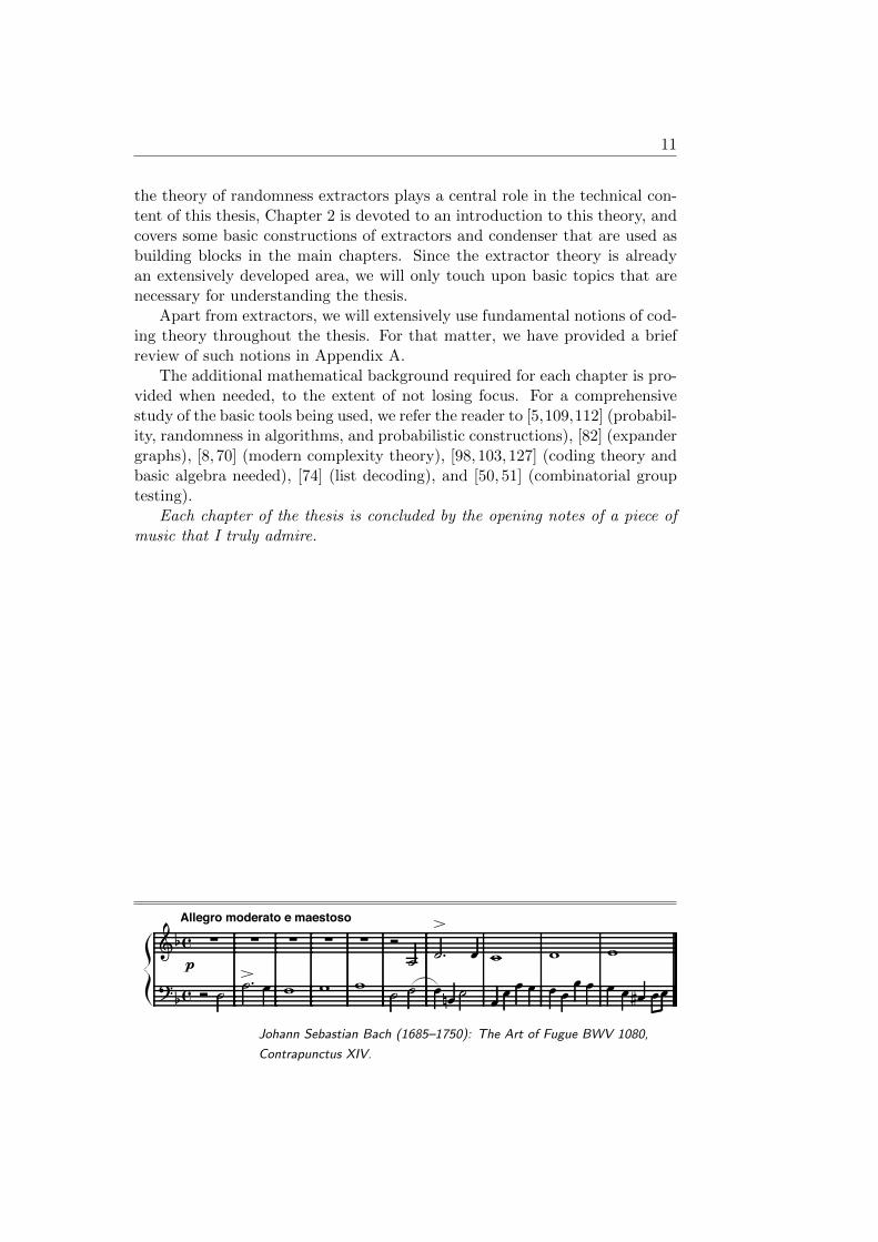
Each chapter of the thesis is concluded by the opening notes of a piece ofmusic that I truly admire.
Allegro moderato e maestoso
Johann Sebastian Bach (1685–1750): The Art of Fugue BWV 1080,
Contrapunctus XIV.
“Art would be useless if theworld were perfect, as manwouldn’t look for harmony butwould simply live in it.”
— Andrei Tarkovsky
Chapter 2
Extractor Theory
Suppose that you are given a possibly biased coin that falls heads some pfraction of times (0 < p < 1) and are asked to use it to “simulate” faircoin flips. A natural approach to solve this problem would be to first try to“learn” the bias p by flipping the coin a large number of times and observingthe fraction of times it falls heads during the experiment, and then using thisknowledge to encode the sequence of biased flips to its information-theoreticentropy.
Remarkably, back in 1951 John von Neumann [159] demonstrated a simpleway to solve this problem without knowing the bias p: flip the coin twice andone of the following cases may occur:
1. The first flip shows Heads and the second Tails: output “H”.
2. The first flip shows Tails and the second Heads: output “T”.
3. Otherwise, repeat the experiment.
Note that the probability that the output symbol is “H” is precisely equalto it being “T”, namely, p(1−p). Thus, the outcome of this process representsa perfectly fair coin toss. This procedure might be somewhat wasteful; forinstance, it is expected to waste half of the coin flips even if p = 1/2 (thatis, if the coin is already fair) and that is the cost we pay for not knowingp. But nevertheless, it transforms an imperfect, not fully known, source ofrandomness into a perfect source of random bits.
This example, while simple, demonstrates the basic idea in what is knownas “extractor theory”. The basic goal in extractor theory is to improve ran-domness, that is, to efficiently transform a “weak” source of randomness intoone with better qualities; in particular, having a higher entropy per symbol.The procedure shown above, seen as a function from the sequence of coin flips
12
2.1. PROBABILITY DISTRIBUTIONS 13
to a Boolean function (over H,T) is known as an extractor. It is called sosince it “extracts” pure randomness from a weak source.
When the distribution of the weak source is known, it is possible to usetechniques from source coding (say Huffman or Arithmetic Coding) to com-press the information to a number of bits very close to its actual entropy,without losing any of the source information. What makes extractor theoryparticularly challenging is the following issues:
1. An extractor knows little about the exact source distribution. Typicallynothing more than a lower bound on the source entropy, and no structureis assumed on the source. In the above example, even though the sourcedistribution was unknown, it was known to be an i.i.d. sequence (i.e.,a sequence of independent, identically distributed symbols). This neednot be the case in general.
2. The output of the extractor must “strongly” resemble a uniform distri-bution (which is the distribution with maximum possible entropy), inthe sense that no statistical test (no matter how complex) should beable to distinguish between the output distribution and a purely ran-dom sequence. Note, for example, that a sequence of n− 1 uniform andindependent bits followed by the symbol “0” has n − 1 bits of entropy,which is only slightly lower than that of n purely random bits (i.e., n).However, a simple statistical test can trivially distinguish between thetwo distributions by only looking at the last bit.
Since extractors and related objects (in particular, lossless condensers)play a central role in the technical core of this thesis, we devote this chapterto a formal treatment of extractor theory, introducing the basic ideas andsome fundamental constructions. In this chapter, we will only cover basicnotions and discuss a few of the results that will be used as building blocks inthe rest of thesis.
2.1 Probability Distributions
2.1.1 Distributions and Distance
In this thesis we will focus on probability distributions over finite domains.Let (Ω,E,X ) be a probability space, where Ω is a finite sample space, E is theset of events (that in our work, will always consist of the set of subsets of Ω),and X is a probability measure. The probability assigned to each outcomex ∈ Ω by X will be denoted by X (x), or PrX (x). Similarly, for an event T ∈ E,we will denote the probability assigned to T by X (T ), or PrX [T ] (when clearfrom the context, we may omit the subscript X ). The support of X is definedas
supp(X ) := x ∈ Ω: X (x) > 0.
14 CHAPTER 2. EXTRACTOR THEORY
A particularly important probability measure is defined by the uniform dis-tribution, which assigns equal probabilities to each element of Ω. We willdenote the uniform distribution over Ω by UΩ, and use the shorthand Un, foran interger n ≥ 1, for U0,1n . We will use the notation X ∼ X to denote thatthe random variable X is drawn from the probability distribution X .
It is often convenient to think about the probability measure as a realvector of dimension |Ω|, whose entries are indexed by the elements of Ω, suchthat the value at the ith entry of the vector is X (i).
An important notion for our work is the distance between distributions.There are several notions of distance in the literature, some stronger thanthe others, and often the most suitable choice depends on the particular ap-plication in hand. For our applications, the most important notion is the `pdistance:
Definition 2.1. Let X and Y be probability distributions on a finite domainΩ. Then for every p ≥ 1, their `p distance, denoted by ‖X −Y‖p, is given by
‖X − Y‖p :=
(∑x∈Ω
|X (x)− Y(y)|p)1/p
.
We extend the distribution to the special case p =∞, to denote the point-wisedistance:
‖X − Y‖∞ := maxx∈Ω|X (x)− Y(y)|.
The distributions X and Y are called ε-close with respect to the `p norm ifand only if ‖X − Y‖p ≤ ε.
We remark that, by the Cauchy-Schwarz inequality, the following relation-ship between `1 and `2 distances holds:
‖X − Y‖2 ≤ ‖X − Y‖1 ≤√|Ω| · ‖X − Y‖2.
Of particular importance is the statistical (or total variation) distance.This is defined as half the `1 distance between the distributions:
‖X − Y‖ := 12‖X − Y‖1.
We may also use the notation dist(X ,Y) to denote the statistical distance. Wecall two distributions ε-close if and only if their statistical distance is at mostε. When there is no risk of confusion, we may extend such notions as distanceto the random variables they are sampled from, and, for instance, talk abouttwo random variables being ε-close.
This is in a sense, a very strong notion of distance since, as the followingproposition suggests, it captures the worst-case difference between the proba-bility assigned by the two distributions to any event:
2.1. PROBABILITY DISTRIBUTIONS 15
Proposition 2.2. Let X and Y be distributions on a finite domain Ω. Then Xand Y are ε-close if and only if for every event T ⊆ Ω, |PrX [T ]−PrY [T ]| ≤ ε.
Proof. Denote by ΩX and ΩY the following partition of Ω:
ΩX := x ∈ Ω: X (x) ≥ Y(x), ΩY := Ω \ TX .
Thus, ‖X − Y‖ = 2(PrX (ΩX ) − PrY(ΩX )) = 2(PrY(ΩY) − PrX (ΩY)). Letp1 := PrX [T ∩ΩX ]−PrY [T ∩ΩX ], and p2 := PrY [T ∩ΩY ]−PrX [T ∩ΩY ]. Bothp1 and p2 are positive numbers, each no more than ε. Therefore,
|PrX
[T ]− PrY
[T ]| = |p1 − p2| ≤ ε.
For the reverse direction, suppose that for every event T ⊆ Ω, |PrX [T ]−PrY [T ]| ≤ ε. Then,
‖X − Y‖1 = |PrX
[ΩX ]− PrY
[ΩX ]|+ |PrX
[ΩY ]− PrY
[ΩY ]| ≤ 2ε.
An equivalent way of looking at an event T ⊆ Ω is by defining a predicateP : Ω → 0, 1 whose set of accepting inputs is T ; namely, P (x) = 1 if andonly if x ∈ T . In this view, Proposition 2.2 can be written in the followingequivalent form.
Proposition 2.3. Let X and Y be distributions on the same finite domain Ω.Then X and Y are ε-close if and only if, for every distinguisher P : Ω→ 0, 1,we have ∣∣∣∣ Pr
X∼X[P (X) = 1]− Pr
Y∼Y[P (Y ) = 1]
∣∣∣∣ ≤ ε.The notion of convex combination of distributions is defined as follows:
Definition 2.4. Let X1,X2, . . . ,Xn be probability distributions over a finitespace Ω and α1, α2, . . . , αn be nonnegative real values that sum up to 1. Thenthe convex combination
α1X1 + α2X2 + · · ·+ αnXn
is a distribution X over Ω given by the probability measure
PrX
(x) :=n∑i=1
αi PrXi
(x),
for every x ∈ Ω.
16 CHAPTER 2. EXTRACTOR THEORY
When regarding probability distributions as vectors of probabilities (withcoordinates indexed by the elements of the sample space), convex combina-tion of distributions is merely a linear combination (specifically, a point-wiseaverage) of their vector forms. Thus intuitively, one expects that if a proba-bility distribution is close to a collection of distributions, it must be close toany convex combination of them as well. This is made more precise in thefollowing proposition.
Proposition 2.5. Let X1,X2, . . . ,Xn be probability distributions, all definedover the same finite set Ω, that are all ε-close to some distribution Y. Thenany convex combination
X := α1X1 + α2X2 + · · ·+ αnXn
is ε-close to Y.
Proof. We give a proof for the case n = 2, which generalizes to any largernumber of distributions by induction. Let T ⊆ Ω be any nonempty subset ofΩ. Then we have
|PrX
[T ]− PrY
[T ]| = |α1 PrX1
[T ] + (1− α1) PrX2
[T ]− PrY
[T ]|
= |α1(PrY
[T ] + ε1) + (1− α1)(PrY
[T ] + ε2)− PrY
[T ]|,
where |ε1|, |ε2| ≤ ε by the assumption that X1 and X2 are ε-close to Y. Hencethe distance simplifies to
|α1ε1 + (1− α1)ε2|,
and this is at most ε.
In a similar manner, it is straightforward to see that a convex combination(1− ε)X + εY is ε-close to X .
Sometimes, in order to show a claim for a probability distribution it may beeasier, and yet sufficient, to write the distribution as a convex combination of“simpler” distributions and then prove the claim for the simpler components.We will examples of this technique when we analyze constructions of extractorsand condensers.
2.1.2 Entropy
A central notion in the study of randomness is related to the informationcontent of a probability distribution. Shannon formalized this notion in thefollowing form:
2.1. PROBABILITY DISTRIBUTIONS 17
Definition 2.6. Let X be a distribution on a finite domain Ω. The Shannonentropy of X (in bits) is defined as
H(X ) :=∑
x∈supp(X )
−X (x) log2X (x) = EX∼X [− log2X (X)].
Intuitively, Shannon entropy quantifies the number of bits required to spec-ify a sample drawn from X on average. This intuition is made more precise, forexample by Huffman coding that suggest an efficient algorithm for encoding arandom variable to a binary sequence whose expected length is almost equalto the Shannon entropy of the random variable’s distribution (cf. [40]). Fornumerous applications in computer science and cryptography, however, thenotion of Shannon entropy–which is an average-case notion–is not well suit-able and a worst-case notion of entropy is required. Such a notion is capturedby min-entropy, defined below.
Definition 2.7. Let X be a distribution on a finite domain Ω. The min-entropy of X (in bits) is defined as
H∞(X ) := minx∈supp(X )
− log2X (x).
Therefore, the min-entropy of a distribution is at least k if and only if thedistribution assigns a probability of at most 2−k to any point of the samplespace (such a distribution is called a k-source). It also immediately follows bydefinitions that a distribution having min-entropy at least k must also have aShannon entropy of at least k. When Ω = 0, 1n, we define the entropy rateof a distribution X on Ω as H∞(X )/n.
A particular class of probability distributions for which the notions ofShannon entropy an min-entropy coincide is flat distributions. A distributionon Ω is called flat if it is uniformly supported on a set T ⊆ Ω; that is, ifit assigns probability 1/|T | to all the points on T and zeros elsewhere. TheShannon- and min-entropies of such a distribution are both log2 |T | bits.
An interesting feature of flat distributions is that their convex combina-tions can define any arbitrary probability distribution with a nice preservenceof the min-entropy, as shown below.
Proposition 2.8. Let K be an integer. Then any distribution X with min-entropy at least logK can be described as a convex combination of flat distri-butions with min-entropy logK.
Proof. Suppose that X is distributed on a finite domain Ω. Any probabilitydistribution on Ω can be regarded as a real vector with coordinates indexed bythe elements of Ω, encoding its probability measure. The set of distributions(pi)i∈Ω with min-entropy at least logK form a simplex
(∀i ∈ Ω) 0 ≤ pi ≤ 1/K,∑i∈Ω pi = 1,
18 CHAPTER 2. EXTRACTOR THEORY
whose corner points are flat distributions. The claim follows since every pointin the simplex can be written as a convex combination of the corner points.
2.2 Extractors and Condensers
2.2.1 Definitions
Intuitively, an extractor is a function that transforms impure randomness; i.e.,a random source containing a sufficient amount of entropy, to an almost uni-form distribution (with respect to a suitable distance measure; e.g., statisticaldistance).
Suppose that a source X is distributed on a sample space Ω := 0, 1nwith a distribution containing at least k bits of min-entropy. The goal isto construct a function f : 0, 1n → 0, 1m such that f(X ) is ε-close tothe uniform distribution Um, for a negligible distance ε (e.g., ε = 2−Ω(n)).Unfortunately, without having any further knowledge on X , this task becomesimpossible. To see why, consider the simplest nontrivial case where k = n− 1and m = 1, and suppose that we have come up with a function f that extractsone almost unbiased coin flip from any k-source. Observe that among the setof pre-images of 0 and 1 under f ; namely, f−1(0) and f−1(1), at least one musthave size 2n−1 or more. Let X be the flat source uniformly distributed on thisset. The distribution X constructed this way has min-entropy at least n − 1yet f(X ) is always constant. In order to alleviate this obvious impossibility,one of the following two solutions is typically considered:
1. Assume some additional structure on the source: In the counterexampleabove, we constructed an opportunistic choice of the source X from thefunction f . However, in general the source obtained this way may turnout to be exceedingly complex and unstructured, and the fact that fis unable to extract any randomness from this particular choice of thesource might be of little concern. A suitable way to model this obser-vation is to require a function f that is expected to extract randomnessonly from a restricted class of randomness sources.
The appropriate restriction in question may depend on the context forwhich the extractor is being used. A few examples that have been con-sidered in the literature include:
• Independent sources: In this case, the source X is restricted to be aproduct distribution with two or more components. In particular,one may assume the source to be the product distribution of r ≥ 2independent random variables X1, . . . , Xr ∈ 0, 1n′ that are eachsampled from an arbitrary k′-source (assuming n = rn′ and k =rk′).
2.2. EXTRACTORS AND CONDENSERS 19
• Affine sources: We assume that the source X is uniformly supportedon an arbitrary translation of an unknown k-dimensional vectorsubspace of1 Fn2 . A further restriction of this class is known as bit-fixing sources. A bit-fixing source is a product distribution of n bits(X1, . . . , Xn) where for some unknown set of coordinates positionsS ⊆ [n] of size k, the variables Xi for i ∈ S are independent anduniform bits, but the rest of the Xi’s are fixed to unknown binaryvalues. In Chapter 3, we will discuss these classes of sources inmore detail.
• Samplable sources: This is a class of sources first studied by Tre-visan and Vadhan [153]. In broad terms, a samplable source is asource X such that a sample from X can produced out of a sequenceof random and independent coin flips by a restricted computationalmodel. For example, one may consider the class of sources of min-entropy k such that for any source X in the class, there is a func-tion f : 0, 1r → 0, 1n, for some r ≥ k, that is computable bypolynomial-size Boolean circuits and satisfies f(Ur) ∼ X .
For restricted classes of sources such as the above examples, there aredeterministic functions that are good extractors for all the sources in thefamily. Such deterministic functions are known as seedless extractors forthe corresponding family of sources. For instance, an affine extractor forentropy k and error ε (in symbols, an affine (k, ε)-extractor) is a mappingf : Fn2 → Fm2 such that for every affine k-source X , the distribution f(X )is ε-close to the uniform distribution Um.
In fact, it is not hard to see that for any family of not “too many” sources,there is a function that extracts almost the entire source entropy of thesources (examples include affine k-sources, samplable k-sources, and twoindependent sources2). This can be shown by a probabilistic argumentthat considers a random function and shows that it achieves the desiredproperties with overwhelming probability.
2. Allow a short random seed : The second solution is to allow extractorto use a small amount of pure randomnness as a “catalyst”. Namely,the extractor is allowed to require two inputs: a sample from the un-known source and a short sequence of random and independent bits thatis called the seed. In this case, it turns out that extracting almost theentire entropy of the weak source becomes possible, without any struc-tural assumptions on the source and using a very short independent seed.Extractors that require an auxiliary random input are called seeded ex-tractors. In fact, an equivalent of looking at seeded extractors is to see
1Throughout the thesis, for a prime power q, we will use the notation Fq to denote thefinite field with q elements.
2For this case, it suffices to count the number of independent flat sources.
20 CHAPTER 2. EXTRACTOR THEORY
them as seedless extractors that assume the source to be structured asa product distribution of two sources: an arbitrary k-source and theuniform distribution.
For the rest of this chapter, we will focus on seeded extractors. Seedlessextractors (especially affine extractors) are treated in Chapter 3. A formaldefinition of (seeded) extractors is as follows.
Definition 2.9. A function f : 0, 1n×0, 1d → 0, 1m is a (k, ε)-extractorif, for every k-source X on 0, 1n, the distribution f(X ,Ud) is ε-close (instatistical distance) to the uniform distribution on 0, 1m. The parametersn, d, k, m, and ε are respectively called the input length, seed length, entropyrequirement, output length, and error of the extractor.
An important aspect of randomness extractors is their computational com-plexity. For most applications, extractors are required to be efficiently com-putable functions. We call an extractor explicit if it is computable in polyno-mial time (in its input length). Though it is rather straightforward to showexistence of good extractors using probabilistic arguments, coming up with anontrivial explicit construction can turn out a much more challenging task.We will discuss and analyze several important explicit constructions of seededextractors in Section 2.3.
Note that, in the above definition of extractors, achieving an output lengthof up to d is trivial: the extractor can merely output its seed, which is guaran-teed to have a uniform distribution! Ideally the output of an extractor mustbe “almost independent” of its seed, so that the extra randomness given inthe seed can be “recycled”. This idea is made precise in the notion of strongextractors given below.
Definition 2.10. A function f : 0, 1n×0, 1d → 0, 1m is a strong (k, ε)-extractor if, for every k-source X on 0, 1n, and random variables X ∼ X ,Z ∼ Ud, the distribution of the random variable (X, f(X,Z)) is ε-close (instatistical distance) to Ud+m.
A fundamental property of strong extractors that is essential for certainapplications is that, the extractor’s output remains close to uniform for almostall fixings of the random seed. This is made clear by an “averaging argument”stated formally in the proposition below.
Proposition 2.11. Consider joint distributions X := (Z,X ) and Y := (Z,Y)that are ε-close, where X and Y are distributions on a finite domain Ω, andZ is uniformly distributed on 0, 1d. For every z ∈ 0, 1d, denote by Xz thedistribution of the second coordinate of X conditioned on the first coordinatebeing equal to z, and similarly define Yz for the distribution Y. Then, forevery δ > 0, at least (1− δ)2d choices of z ∈ 0, 1d must satisfy
‖Xz − Yz‖ ≤ ε/δ.
2.2. EXTRACTORS AND CONDENSERS 21
Proof. Clearly, for every ω ∈ Ω and z ∈ 0, 1d, we have Xz(ω) = 2dX (z, ω)and similarly, Yz(ω) = 2dY(z, ω). Moreover from the definition of statisticaldistance, ∑
z∈0,1d
∑ω∈Ω
|X (z, ω)− Y(z, ω)| ≤ 2ε.
Therefore, ∑z∈0,1d
∑ω∈Ω
|Xz(ω)− Yz(ω)| ≤ 2d+1ε,
which can be true only if for at least (1 − δ) fraction of the choices of z, wehave ∑
ω∈Ω
|Xz(ω)− Yz(ω)| ≤ 2ε/δ,
or in other words,‖Xz − Yz‖ ≤ ε/δ.
This shows the claim.
Thus, according to Proposition 2.11, for a strong (k, ε)-extractor
f : 0, 1n × 0, 1d → 0, 1m
and a k-source X , for 1−√ε fraction of the choices of z ∈ 0, 1d, the distri-bution f(X , z) must be ε-close to uniform.
Extractors are specializations of the more general notion of randomnesscondensers. Intuitively, a condenser transforms a given weak source of ran-domness into a “more purified” but possibly imperfect source. In general, theoutput entropy of a condenser might be substantially less than the input en-tropy but nevertheless, the output is generally required to have a substantiallyhigher entropy rate. For the extremal case of extractors, the output entropyrate is required to be 1 (since the output is required to be an almost uni-form distribution). Same as extractors, condensers can be seeded or seedless,and also seeded condensers can be required to be strong (similar to strongextractors). Below we define the general notion of strong, seeded condensers.
Definition 2.12. A function f : 0, 1n×0, 1d → 0, 1m is a strong k →ε k′
condenser if for every distribution X on 0, 1n with min-entropy at least k,random variable X ∼ X and a seed Y ∼ Ud, the distribution of (Y, f(X,Y )) isε-close to a distribution (Ud,Z) with min-entropy at least d+ k′. The param-eters k, k′, ε, k − k′, and m− k′ are called the input entropy, output entropy,error, the entropy loss and the overhead of the condenser, respectively. Acondenser is explicit if it is polynomial-time computable.
Similar to strong extractors, strong condensers remain effective under al-most all fixings of the seed. This follows immediately from Proposition 2.11and is made explicit by the following corollary:
22 CHAPTER 2. EXTRACTOR THEORY
Corollary 2.13. Let f : 0, 1n × 0, 1d → 0, 1m be a strong k →ε k′
condenser. Consider an arbitrary parameter δ > 0 and a k-source X . Then,for all but at most a δ fraction of the choices of z ∈ 0, 1d, the distributionf(X , z) is (ε/δ)-close to a k′-source.
Typically, a condenser is only interesting if the output entropy rate k′/mis considerably larger than the input entropy rate k/n. From the above defi-nition, an extractor is a condenser with zero overhead. Another extremal casecorresponds to the case where the entropy loss of the condenser is zero. Such acondenser is called lossless. We will use the abbreviated term (k, ε)-condenserfor a lossless condenser with input entropy k (equal to the output entropy)and error ε. Moreover, if a function is a (k0, ε)-condenser for every k0 ≤ k, it iscalled a (≤ k, ε)-condenser. Most known constructions of lossless condensers(and in particular, all constructions used in this thesis) are (≤ k, ε)-condensersfor their entropy requirement k.
Traditionally, lossless condensers have been used as intermediate buildingblocks for construction of extractors. Having a good lossless condenser avail-able, for construction of extractors it would suffice to focus on the case wherethe input entropy is large. Nevertheless, lossless condensers have been provedto be useful for a variety of applications, some of which we will discuss in thisthesis.
2.2.2 Almost-Injectivity of Lossless Condensers
Intuitively, an extractor is an almost “uniformly surjective” mapping. Thatis, the extractor mapping distributes the probability mass of the input sourcealmost evenly among the elements of its range.
On the other hand, a lossless condenser preserves the entire source entropyon its output and intuitively, must be an almost injective function when re-stricted to the domain defined by the input distribution. In other words, in themapping defined by the condenser “collisions” rarely occur and in this view,lossless condensers are useful “hashing” tools. In this section we formalize thisintuition through a simple practical application.
Given a source X and a function f , if f(X ) has the same entropy as thatof X (or in other words, if f is a perfectly lossless condenser for X ) we expectthat from the outcome of the function, its input when sampled from X mustbe reconstructible. For flat distributions (that is, those that are uniform ontheir support) and considering an error for the condenser, this is shown in thefollowing proposition. We will use this simple fact several times throughoutthe thesis.
Proposition 2.14. Let X be a flat distribution with min-entropy logK overa finite sample space Ω and f : Ω→ Γ be a mapping to a finite set Γ.
2.2. EXTRACTORS AND CONDENSERS 23
1. If f(X ) is ε-close to having min-entropy logK, then there is a set T ⊆ Γof size at least (1− 2ε)K such that
(∀y ∈ T and ∀x, x′ ∈ supp(X )) f(x) = y ∧ f(x′) = y ⇒ x = x′.
2. Suppose |Γ| ≥ K. If f(X ) has a support of size at least (1− ε)K, thenit is ε-close to having min-entropy logK.
Proof. Suppose that X is uniformly supported on a set S ⊆ Ω of size K, anddenote by µ the distribution f(X ) over Γ. For each y ∈ Γ, define
ny := |x ∈ supp(X ) : f(x) = y|.
Moreover, define T := y ∈ Γ: ny = 1, and similarly, T ′ := y ∈ Γ: ny ≥ 2.Observe that for each y ∈ Γ we have µ(y) = ni/K, and also supp(µ) = T ∪T ′.Thus,
(2.1) |T |+∑y∈T ′
ny = K.
Now we show the first assertion. Denote by µ′ a distribution on Γ with min-entropy K that is ε-close to µ, which is guaranteed to exist by the assumption.The fact that µ and µ′ are ε-close implies that∑
y∈T ′|µ(y)− µ′(y)| ≤ ε⇒
∑y∈T ′
(ny − 1) ≤ εK.
In particular, this means that |T ′| ≤ εK (since by the choice of T ′, for eachy ∈ T ′ we have ny ≥ 2). Furthermore,∑
y∈T ′(ny − 1) ≤ εK ⇒
∑y∈T ′
ny ≤ εK + |T ′| ≤ 2εK.
This combined with (2.1) gives
|T | = K −∑y∈T ′
ny ≥ (1− 2ε)K
as desired.For the second part, observe that |T ′| ≤ εK. Let µ′ be any flat distribution
with a support of size K that contains the support of µ. The statisticaldistance between µ and µ′ is equal to the difference between the probabilitymass of the two distributions on those elements of Γ to which µ′ assigns abigger probability, namely,
1
K(supp(µ′)−supp(µ)) =
∑y∈T ′(ny − 1)
K=
∑y∈T ′ ny − |T ′|
K=K − |T | − |T ′|
K,
where we have used (2.1) for the last equality. But |T | + |T ′| = |supp(µ)| ≥(1− ε)K, giving the required bound.
24 CHAPTER 2. EXTRACTOR THEORY
As a simple application of this fact, consider the following “source coding”problem. Suppose that Alice wants to send a message x to Bob through anoiseless communication channel, and that the message is randomly sampledfrom a distribution X . Shannon’s source coding theorem roughly states that,there is a compression scheme that encodes x to a binary sequence y of lengthH(X) bits on average, where H(·) denotes the Shannon entropy, such that Bobcan perfectly reconstruct y from x (cf. [40, Chapter 5]). If the distribution Xis known to both Alice and Bob, they can use an efficient coding scheme suchas Huffman codes or Arithmetic coding to achieve this bound (up to a smallconstant bits of redundancy).
On the other hand, certain universal compression schemes are known thatguarantee an optimal compression provided that X satisfies certain statisti-cal properties. For instance, Lempel-Ziv coding achieves the optimum com-pression rate without exact knowledge of X provided that is defined by astationary, ergodic process (cf. [40, Chapter 13]).
Now consider a situation where the distribution X is arbitrary but onlyknown to the receiver Bob. In this case, it is known that there is no wayfor Alice to substantially compress her information without interaction withBob [2]. On the other hand, if we allow interaction, Bob may simply send adescription of the probability distribution X to Alice so she can use a classicalsource coding scheme to compress her information at the entropy.
Interestingly, it turns out that this task is still possible if the amount of in-formation sent to Alice is substantially lower than what needed to fully encodethe probability distribution X . This is particularly useful if the bandwidthfrom Alice to Bob is substantially lower than that of the reverse direction(consider, for example, an ADSL connection) and for this reason, the problemis dubbed as the asymmetric communication channel problem. In particular,Watkinson et al. [160] obtain a universal scheme with H(X ) + 2 bits of com-munication from Alice to Bob and n(H(X ) + 2) bits from Bob to Alice, wheren is the bit-length of the message. Moreover, Adler et al. [1] obtain stronglower bounds on the number of rounds of communication between Alice andBob.
Now let us impose a further restriction on X that it is uniformly sup-ported on a set S ⊆ 0, 1n, and Alice knows nothing about S but its size.If we disallow interaction between Alice and Bob, there would still be no de-terministic way for Alice to deterministically compress her message. This iseasy to observe by noting that any deterministic, and compressing, functionϕ : 0, 1n → 0, 1m, where m < n, has an output value with as many as2n−m pre-images, and an adversarial choice of S that concentrates on the setof such pre-images would force the compression scheme to fail.
However, let us allow the encoding scheme to be randomized, and err witha small probability over the randomness of the scheme and the message. In thiscase, Alice can take a strong lossless condenser f : 0, 1n×0, 1d → 0, 1mfor input entropy k := log |S|, choose a uniformly random seed z ∈ 0, 1d,
2.3. CONSTRUCTIONS 25
and transmit y := (z, f(x, z)) to Bob. Now we argue that Bob will be able torecover x from y.
Let ε denote the error of the condenser. Since f is a lossless condenser forX , we know that, for Z ∼ Ud and X ∼ X , the distribution of (Z, f(X,Z)) isε-close to some distribution (Ud,Y), with min-entropy at least d + k. Thusby Corollary 2.13 it follows that, for at least 1 − √ε fraction of the choicesof z ∈ 0, 1d, the distribution Yz := f(X , z) is
√ε-close to having min-
entropy k. For any such “good seed” z, Proposition 2.14 implies that onlyfor at most 2
√ε fraction of the message realizations x ∈ S can the encoding
f(x, z) be confused with a different encoding f(x′, z) for some x′ ∈ S, x′ 6= x.Altogether we conclude that, from the encoding y, Bob can uniquely deducex with probability at least 1 − 3
√ε, where the probability is taken over the
randomness of the seed and the message distribution X .The amount of communication in this encoding scheme is m+d bits. Using
an optimal lossless condenser for f , the encoding length becomes k+O(log n)with a polynomially small (in n) error probability (where the exponent ofthe polynomial is arbitrary and affects the constant in the logarithmic term).On the other hand, with the same error probability, the explict condenser ofTheorem 4.19 would give an encoding length k + O(log3 n). Moreover, theexplicit condenser of Theorem 2.22 results in length k(1 + α) +Oα(log n) forany arbitrary constant α > 0.
2.3 Constructions
We now turn to explicit constructions of strong extractors and lossless con-densers.
Using probabilistic arguments, Radhakrishan and Ta-Shma [122] showedthat, for every k, n, ε, there is a strong (k, ε)-extractor with seed length d =log(n − k) + 2 log(1/ε) + O(1) and output length m = k − 2 log(1/ε) − O(1).In particular, a random function achieves these parameters with probability1−o(1). Moreover, their result show that this trade-off is almost the best onecan hope for.
Similar trade-offs are known for lossless condensers as well. Specifically, theprobabilistic construction of Radhakrishan and Ta-Shma has been extendedto the case of lossless condensers by Capalbo et al. [23], where they show thata random function is with high probability a strong lossless (k, ε)-condenserwith seed length d = log n + log(1/ε) + O(1) and output length m = k +log(1/ε) +O(1). Moreover, this tradeoff is almost optimal as well.
In this section, we introduce some important explicit constructions of bothextractors and lossless condensers that are used as building blocks of variousconstructions in the thesis. In particular, we will discuss extractors and losslesscondensers obtained by the Leftover Hash Lemma, Trevisan’s extractor, anda lossless condenser due to Guruswami, Umans, and Vadhan.
26 CHAPTER 2. EXTRACTOR THEORY
2.3.1 The Leftover Hash Lemma
One of the foremost explicit constructions of extractors is given by the Left-over Hash Lemma first stated by Impagliazzo, Levin, and Luby [84]. Thisextractor achieves an optimal output length m = k − 2 log(1/ε) albeit witha substantially large seed length d = n. Moreover, the extractor is a linearfunction for every fixing of the seed. In its general form, the lemma statesthat any universal family of hash functions can be transformed into an ex-plicit extractor. The universality property required by the hash functions iscaptured by the following definition.
Definition 2.15. A family of functionsH = h1, . . . , hD where hi : 0, 1n →0, 1m for i = 1, . . . , D is called universal if, for every fixed choice of x, x′ ∈0, 1n such that x 6= x′ and a uniformly random i ∈ [D] := 1, . . . , D wehave
Pri
[hi(x) = hi(x′)] ≤ 2−m.
One of the basic examples of universal hash families is what we call thelinear family, defined as follows. Consider an arbitrary isomorphism ϕ : Fn2 →F2n between the vector space Fn2 and the extension field F2n , and let 0 < m ≤n be an arbitrary integer. The linear family Hlin is the set hα : α ∈ F2n ofsize 2n that contains a function for each element of the extension field F2n .For each α, the mapping hα is given by
hα(x) := (y1, . . . , ym), where (y1, . . . , yn) := ϕ−1(α · ϕ(x)).
Observe that each function hα can be expressed as a linear mapping from Fn2to Fm2 . Below we show that this family is pairwise independent.
Proposition 2.16. The linear family Hlin defined above is universal.
Proof. Let x, x′ be different elements of F2n . Consider the mapping f : F2n →Fm2 defined as
f(x) := (y1, . . . , ym), where (y1, . . . , yn) := ϕ−1(x),
which truncates the binary representation of a field element from F2n to mbits. The probability we are trying to estimate in Definition 2.15 is, for auniformly random α ∈ F2n ,
Prα∈F2n
[f(α · x) = f(α · x′)] = Prα∈F2n
[f(α · (x− x′)) = 0].
But note that x − x′ is a nonzero element of F2n , and thus, for a uniformlyrandom α, the random variable αx is uniformly distributed on F2n . It followsthat
Prα∈F2n
[f(α · (x− x′)) = 0] = 2−m,
implying that Hlin is a universal family.
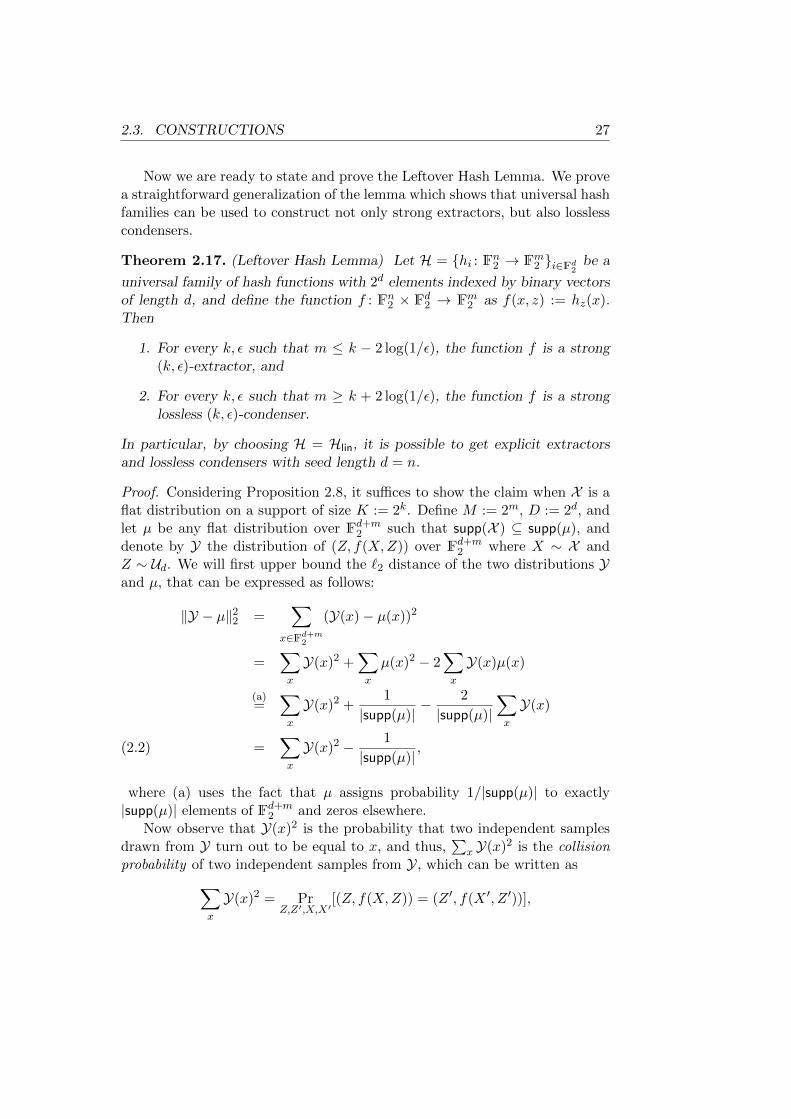
2.3. CONSTRUCTIONS 27
Now we are ready to state and prove the Leftover Hash Lemma. We provea straightforward generalization of the lemma which shows that universal hashfamilies can be used to construct not only strong extractors, but also losslesscondensers.
Theorem 2.17. (Leftover Hash Lemma) Let H = hi : Fn2 → Fm2 i∈Fd2 be a
universal family of hash functions with 2d elements indexed by binary vectorsof length d, and define the function f : Fn2 × Fd2 → Fm2 as f(x, z) := hz(x).Then
1. For every k, ε such that m ≤ k − 2 log(1/ε), the function f is a strong(k, ε)-extractor, and
2. For every k, ε such that m ≥ k + 2 log(1/ε), the function f is a stronglossless (k, ε)-condenser.
In particular, by choosing H = Hlin, it is possible to get explicit extractorsand lossless condensers with seed length d = n.
Proof. Considering Proposition 2.8, it suffices to show the claim when X is aflat distribution on a support of size K := 2k. Define M := 2m, D := 2d, andlet µ be any flat distribution over Fd+m
2 such that supp(X ) ⊆ supp(µ), anddenote by Y the distribution of (Z, f(X,Z)) over Fd+m
2 where X ∼ X andZ ∼ Ud. We will first upper bound the `2 distance of the two distributions Yand µ, that can be expressed as follows:
‖Y − µ‖22 =∑
x∈Fd+m2
(Y(x)− µ(x))2
=∑x
Y(x)2 +∑x
µ(x)2 − 2∑x
Y(x)µ(x)
(a)=
∑x
Y(x)2 +1
|supp(µ)| −2
|supp(µ)|∑x
Y(x)
=∑x
Y(x)2 − 1
|supp(µ)| ,(2.2)
where (a) uses the fact that µ assigns probability 1/|supp(µ)| to exactly|supp(µ)| elements of Fd+m
2 and zeros elsewhere.Now observe that Y(x)2 is the probability that two independent samples
drawn from Y turn out to be equal to x, and thus,∑
x Y(x)2 is the collisionprobability of two independent samples from Y, which can be written as∑
x
Y(x)2 = PrZ,Z′,X,X′
[(Z, f(X,Z)) = (Z ′, f(X ′, Z ′))],
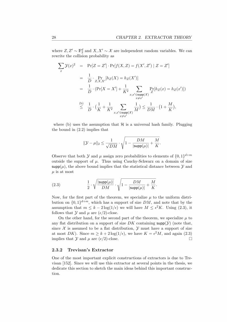
28 CHAPTER 2. EXTRACTOR THEORY
where Z,Z ′ ∼ Fd2 and X,X ′ ∼ X are independent random variables. We canrewrite the collision probability as∑
x
Y(x)2 = Pr[Z = Z ′] · Pr[f(X,Z) = f(X ′, Z ′) | Z = Z ′]
=1
D· PrZ,X,X′
[hZ(X) = hZ(X ′)]
=1
D· (Pr[X = X ′] +
1
K2
∑x,x′∈supp(X )
x 6=x′
PrZ
[hZ(x) = hZ(x′)])
(b)
≤ 1
D·( 1
K+
1
K2
∑x,x′∈supp(X )
x 6=x′
1
M
)≤ 1
DM·(1 +
M
K
),
where (b) uses the assumption that H is a universal hash family. Pluggingthe bound in (2.2) implies that
‖Y − µ‖2 ≤1√DM
·√
1− DM
|supp(µ)| +M
K.
Observe that both Y and µ assign zero probabilities to elements of 0, 1d+m
outside the support of µ. Thus using Cauchy-Schwarz on a domain of sizesupp(µ), the above bound implies that the statistical distance between Y andµ is at most
(2.3)1
2·√|supp(µ)|DM
·√
1− DM
|supp(µ)| +M
K.
Now, for the first part of the theorem, we specialize µ to the uniform distri-bution on 0, 1d+m, which has a support of size DM , and note that by theassumption that m ≤ k − 2 log(1/ε) we will have M ≤ ε2K. Using (2.3), itfollows that Y and µ are (ε/2)-close.
On the other hand, for the second part of the theorem, we specialize µ toany flat distribution on a support of size DK containing supp(Y) (note that,since X is assumed to be a flat distribution, Y must have a support of sizeat most DK). Since m ≥ k + 2 log(1/ε), we have K = ε2M , and again (2.3)implies that Y and µ are (ε/2)-close.
2.3.2 Trevisan’s Extractor
One of the most important explicit constructions of extractors is due to Tre-visan [152]. Since we will use this extractor at several points in the thesis, wededicate this section to sketch the main ideas behind this important construc-tion.
2.3. CONSTRUCTIONS 29
Trevisan’s extractor can be thought of as an “information-theoretic” vari-ation of Nisan-Wigderson’s pseudorandom generator that will be discussed indetail in Chapter 6. For the purpose of this exposition, we will informallydemonstrate how Nisan-Wigderson’s generator works and then discuss Tre-visan’s extractor from a coding-theoretic perspective.
Loosely speaking, a pseudorandom generator is an efficient and determin-istic function (where the exact meaning of “efficient” may vary depending onthe context) that transforms a statistically uniform distribution on d bits toa distribution on m bits, for some m d, that “looks random” to any “re-stricted” distinguisher. Again the precise meaning of “looking random” andthe exact restriction of the distinguisher may vary. In particular, we requirethe output distribution X of the pseudorandom generator to be such that, forevery restricted distinguisher D : 0, 1m → 0, 1, we have∣∣∣∣ Pr
X∼X[D(X) = 1]− Pr
Y∼Um[D(Y ) = 1]
∣∣∣∣ ≤ ε,where ε is a negligible bias. Recall that, in in light of Proposition 2.3, thisis very close to what we expect from the output distribution of an extrac-tor, except that for the case of pseudorandom generators the distinguisher Dcannot be an arbitrary function. Indeed, when m > d, the output distribu-tion of a pseudorandom generator cannot be close to uniform and is alwaysdistinguishable by some distinguisher. The main challenge in constructionof a pseudorandom gnerator is to exclude the possibility of such a distin-guisher to be included in the restricted class of functions into consideration.As a concrete example, one may require a pseudorandom generator to be apolynomial-time computable function whose output is a sequence of lengthd2 that is indistinguishable by linear-sized Boolean circuits with a bias betterthan d−2.
Nisan and Wigderson observed that the hardness of distinguishing theoutput distribution from uniform can be derived from a hardness assumptionthat is inherent in the way the pseudorandom generator itself is computed.In a way, their construction shows how to “trade” computational hardnesswith pseudorandomness. In a simplified manner, a special instantiation ofthis generator can be described as follows: Suppose that a Boolean predicatef : 0, 1d → 0, 1 is hard to compute on average by “small” Boolean circuits;meaning that no circuit consisting of a sufficiently small number of gates (asdetermined by a security parameter) is able to compute f substantially betterthan a trivial circuit that always outputs a constant value. Then, given arandom seed Z ∈ 0, 1d, the sequence (Z, f(Z)) is pseudorandom for smallcircuits. The reason can be seen by contradiction. Let us suppose that forsome distinguisher D, we have∣∣∣∣ Pr
X∼X[D(X) = 1]− Pr
Y∼Um[D(Y ) = 1]
∣∣∣∣ > ε.
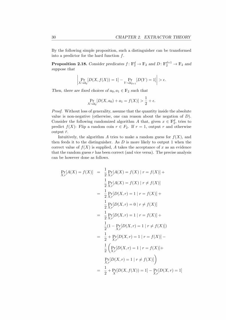
30 CHAPTER 2. EXTRACTOR THEORY
By the following simple proposition, such a distinguisher can be transformedinto a predictor for the hard function f .
Proposition 2.18. Consider predicates f : Fd2 → F2 and D : Fd+12 → F2 and
suppose that ∣∣∣∣ PrX∼Ud
[D(X, f(X)) = 1]− PrY∼Ud+1
[D(Y ) = 1]
∣∣∣∣ > ε.
Then, there are fixed choices of a0, a1 ∈ F2 such that
PrX∼Ud
[D(X, a0) + a1 = f(X)] >1
2+ ε.
Proof. Without loss of generality, assume that the quantity inside the absolutevalue is non-negative (otherwise, one can reason about the negation of D).Consider the following randomized algorithm A that, given x ∈ Fd2, tries topredict f(X): Flip a random coin r ∈ F2. If r = 1, output r and otherwiseoutput r.
Intuitively, the algorithm A tries to make a random guess for f(X), andthen feeds it to the distinguisher. As D is more likely to output 1 when thecorrect value of f(X) is supplied, A takes the acceptance of x as an evidencethat the random guess r has been correct (and vice versa). The precise analysiscan be however done as follows.
PrX,r
[A(X) = f(X)] =1
2PrX,r
[A(X) = f(X) | r = f(X)] +
1
2PrX,r
[A(X) = f(X) | r 6= f(X)]
=1
2PrX,r
[D(X, r) = 1 | r = f(X)] +
1
2PrX,r
[D(X, r) = 0 | r 6= f(X)]
=1
2PrX,r
[D(X, r) = 1 | r = f(X)] +
1
2(1− Pr
X,r[D(X, r) = 1 | r 6= f(X)])
=1
2+ PrX,r
[D(X, r) = 1 | r = f(X)]−
1
2
(PrX,r
[D(X, r) = 1 | r = f(X)]+
PrX,r
[D(X, r) = 1 | r 6= f(X)]
)=
1
2+ Pr
X[D(X, f(X)) = 1]− Pr
X,r[D(X, r) = 1]
2.3. CONSTRUCTIONS 31
>1
2+ ε.
Therefore, by averaging, for some fixed choice of r the probability mustremain above 1
2 + ε, implying that one of the functions D(X, 0), D(X, 1) ortheir negations must be as good a predictor for f(X) as A is.
Since the complexity of the predictor is about the same as that of thedistinguisher D, and by assumption f cannot be computed by small circuits,we conclude that the outcome of the generator must be indistinguishable fromuniform by small circuits. Nisan and Wigderson generalized this idea to ob-tain generators that output a long sequence of bits that is indistinguishablefrom having a uniform distribution. In order to obtain more than one pseu-dorandom bit from the random seed, they evaluate the hard function f oncarefully chosen subsequences of the seed (for this to work, the input lengthof f is assumed to be substantially smaller than the seed length d).
An important observation in Trevisan’s work is that Nisan-Wigderson’spseudorandom generator is a black-box construction. Namely, the generatormerely computes the hard function f at suitably chosen points without caringmuch about how this computation is implemented. Similarly, the analysis usesthe distinguisher D as a black-box. If f is computable in polynomial time,then so is the generator (assuming that it outputs polynomially many bits),and if f is hard against small circuits, the class of circuits of about the samesize must be fooled by the generator.
How can we obtain an extractor from Nisan-Wigderson’s construction? Re-call that the output distribution of an extractor must be indistinguishable fromuniform by all circuits, and not only small ones. Adapting Nisan-Wigderson’sgenerator for this requirement means that we will need a function f that ishard for all circuits, something which is obviously impossible. However, thisproblem can be resolved if we take many hard functions instead of one, andenforce the predictor to simultaneously predict all functions with a reason-able bias. More precisely, statistical indistinguishability can be obtained ifthe function f is sampled from a random distribution, and that is exactly howTrevisan’s extractor uses the supplied weak source. In particular, the extrac-tor regards the sequence obtained from the weak source as the truth table ofa randomly chosen function, and then applies Nisan-Wigderson’s constructionrelative to that function.
The exact description of the extractor is given in Construction 2.1. Theextractor assumes the existence of a suitable list-decodable code (see Ap-pendix A for the terminology) as well as a combinatorial design. Intuitively,a combinatorial design is a collection of subsets of a universe such that theirpairwise intersections are small. We will study designs more closely in Chap-ter 4. In order to obtain a polynomial-time computable extractor, we need an
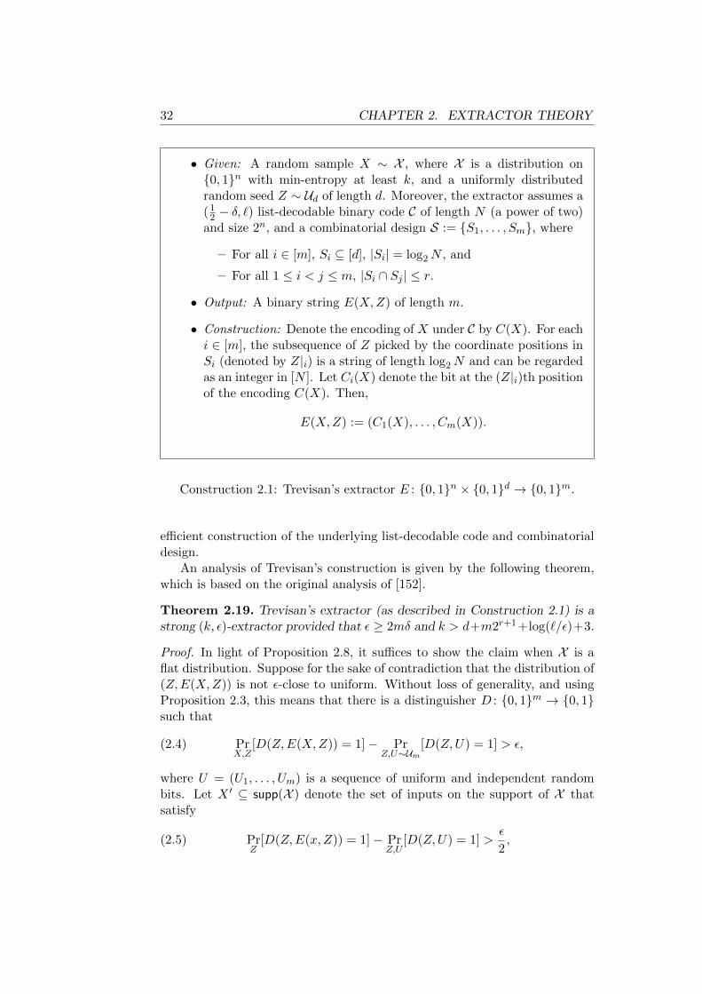
32 CHAPTER 2. EXTRACTOR THEORY
• Given: A random sample X ∼ X , where X is a distribution on0, 1n with min-entropy at least k, and a uniformly distributedrandom seed Z ∼ Ud of length d. Moreover, the extractor assumes a(1
2 − δ, `) list-decodable binary code C of length N (a power of two)and size 2n, and a combinatorial design S := S1, . . . , Sm, where
– For all i ∈ [m], Si ⊆ [d], |Si| = log2N , and
– For all 1 ≤ i < j ≤ m, |Si ∩ Sj | ≤ r.
• Output: A binary string E(X,Z) of length m.
• Construction: Denote the encoding of X under C by C(X). For eachi ∈ [m], the subsequence of Z picked by the coordinate positions inSi (denoted by Z|i) is a string of length log2N and can be regardedas an integer in [N ]. Let Ci(X) denote the bit at the (Z|i)th positionof the encoding C(X). Then,
E(X,Z) := (C1(X), . . . , Cm(X)).
Construction 2.1: Trevisan’s extractor E : 0, 1n × 0, 1d → 0, 1m.
efficient construction of the underlying list-decodable code and combinatorialdesign.
An analysis of Trevisan’s construction is given by the following theorem,which is based on the original analysis of [152].
Theorem 2.19. Trevisan’s extractor (as described in Construction 2.1) is astrong (k, ε)-extractor provided that ε ≥ 2mδ and k > d+m2r+1+log(`/ε)+3.
Proof. In light of Proposition 2.8, it suffices to show the claim when X is aflat distribution. Suppose for the sake of contradiction that the distribution of(Z,E(X,Z)) is not ε-close to uniform. Without loss of generality, and usingProposition 2.3, this means that there is a distinguisher D : 0, 1m → 0, 1such that
(2.4) PrX,Z
[D(Z,E(X,Z)) = 1]− PrZ,U∼Um
[D(Z,U) = 1] > ε,
where U = (U1, . . . , Um) is a sequence of uniform and independent randombits. Let X ′ ⊆ supp(X ) denote the set of inputs on the support of X thatsatisfy
(2.5) PrZ
[D(Z,E(x, Z)) = 1]− PrZ,U
[D(Z,U) = 1] >ε
2,
2.3. CONSTRUCTIONS 33
Observe that the size of X ′ must be at least ε2 |supp(X )| = ε2k−1, since other-
wise (2.4) cannot be satisfied. In the sequel, fix any x ∈ X ′.For i = 0, . . . ,m, define a hybrid sequence Hi as the random variable
Hi := (Z,C1(x), . . . , Ci(x), Ui+1, . . . , Um). Thus, H0 is a uniformly randombit sequence and Hm has the same distribution as (Z,E(x, Z)). For i ∈ [m],define
δi := Pr[D(Hi) = 1]− Pr[D(Hi−1) = 1],
where the probability is taken over the randomness of Z and U . Now we canrewrite (2.5) as
Pr[D(Hm) = 1]− Pr[D(H0) = 1] >ε
2,
or equivalently,m∑i=1
δi >ε
2.
Therefore, for some i ∈ [m], we must have δi > ε/(2m) =: ε′. Fix such an i,and recall that we have
(2.6) Pr[D(Z,C1(x), . . . , Ci(x), Ui+1, . . . , Um) = 1]−Pr[D(Z,C1(x), . . . , Ci−1(x), Ui, . . . , Um) = 1] > ε′.
Now observe that there is a fixing Ui+1 = ui+1, . . . , Um = um of the randombits Ui+1, . . . , Um that preserves the above bias. In a similar way as we definedthe subsequence Z|i, denote by Z |i the subsequence of Z obtained by removingthe coordinate positions of Z picked by Si. Now we note that Ci(x) dependsonly on x and Z|i and is in particular independent of Z |i. Furthermore, onecan fix Z |i (namely, the portion of the random seed outside Si) such that thebias in (2.6) is preserved. In other words, there is a string z′ ∈ 0, 1d−|Si|such that
Pr[D(Z,C1(x), . . . , Ci(x), ui+1, . . . , um) = 1 | (Z |i) = z′]−Pr[D(Z,C1(x), . . . , Ci−1(x), Ui, ui+1, . . . , um) = 1 | (Z |i) = z′] > ε′,
where the randomness is now only over Ui and Z|i, and all other randomvariables are fixed to their appropriate values. Now, Proposition 2.18 canbe used to show that, under the above fixings, there is a fixed choice of bitsa0, a1 ∈ F2 such that D can be transformed into a predictor for Ci(x); namely,so that
PrZ
[D(Z,C1(x), . . . , Ci−1(x), a0, ui+1, . . . , um)+a1 = Ci(x) | (Z |i) = z′] >1
2+ε′.
Since Z|i is a uniformly distributed random variable, the above probability canbe interpreted in coding-theoretic ways as follows: By running through all the
34 CHAPTER 2. EXTRACTOR THEORY
N possibilities of Z|i, the predictor constructed from D can correctly recoverthe encoding C(x) at more than 1
2 + ε′ fraction of the positions. Therefore,the distinguisher D can be transformed into a word w ∈ FN2 that has anagreement above 1
2 + ε2m with C(x).
Now a crucial observation is that the word w can be obtained from Dwithout any knowledge of x, as long a correct “advice” string consisting ofthe appropriate fixings of i, ui+1, . . . , um, a0, a1, z
′, and the truth tables ofC1(x), . . . , Ci−1(x) as functions of Z|i are available. Here is where the smallintersection property of the design S comes to play: Each Cj(x) (when j 6= i)depends on at most r of the bits in Z|i, and therefore, Cj(x) as a function ofZ|i can be fully described by its evaluation on at most 2r points (that can bemuch smaller than 2|Si| = N). This means that the number of possibilities forthe advice string is at most
m · 2m · 4 · 2d−logN · 2m2r =m
N· 2d+m(2r+1)+2 ≤ 2d+m(2r+1)+2 =: T.
Therefore, regardless of the choice of x ∈ X ′, there are words w1, . . . , wT ∈ FN2(one for each possibility of the advice string) such that at least one (corre-sponding to the “correct” advice) has an agreement better than 1
2 + ε′ withC(x). This, in turn, implies that there is a set X ′′ ⊆ X ′ of size at least|X ′|/T ≥ ε2k−1/T and a fixed j ∈ [T ] such that, for every x ∈ X ′′, the code-word C(x) has an agreement better than 1
2 + ε′ with wj . As long as δ ≤ ε′,the number of such codewords can be at most ` (by the list-decodability ofC), and we will reach to the desired contradiction (completing the proof) ifthe list size ` is small enough; specifically, if
` <ε2k−1
T,
which holds by the assumption of the theorem.
By an appropriate choice of the underlying combinatorial design S andthe list-decodable code C (namely, concatenation of the Reed-Solomon codeand the Hadamard code as described in Section A.5), Trevisan [152] obtaineda strong extractor with output length k1−α, for any fixed constant α > 0,and seed length d = O(log2(n/ε)/ logk). In a subsequent work, Raz, Reingoldand Vadhan observed that a weaker notion of combinatorial designs sufficefor this construction to work. Using this idea and a careful choice of the list-decodable code C, they managed to improve Trevisan’s extractor so that itextracts almost the entire source entropy. Specifically, their imrpovement canbe summarized as follows.
Theorem 2.20. [123] For every n, k,m ∈ N, (m ≤ k ≤ n) and ε > 0, thereis an explicit strong (k, ε)-extractor Tre : 0, 1n × 0, 1d → 0, 1m withd = O(log2(n/ε) · log(1/α)), where α := k/(m − 1) − 1 must be less than1/2.
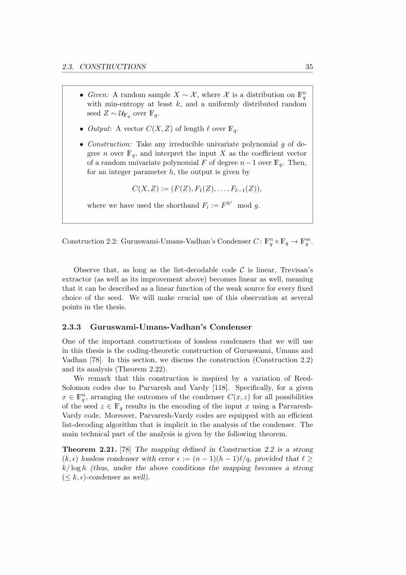
2.3. CONSTRUCTIONS 35
• Given: A random sample X ∼ X , where X is a distribution on Fnqwith min-entropy at least k, and a uniformly distributed randomseed Z ∼ UFq over Fq.
• Output: A vector C(X,Z) of length ` over Fq.
• Construction: Take any irreducible univariate polynomial g of de-gree n over Fq, and interpret the input X as the coefficient vectorof a random univariate polynomial F of degree n−1 over Fq. Then,for an integer parameter h, the output is given by
C(X,Z) := (F (Z), F1(Z), . . . , F`−1(Z)),
where we have used the shorthand Fi := F hi
mod g.
Construction 2.2: Guruswami-Umans-Vadhan’s Condenser C : Fnq ×Fq → Fmq .
Observe that, as long as the list-decodable code C is linear, Trevisan’sextractor (as well as its improvement above) becomes linear as well, meaningthat it can be described as a linear function of the weak source for every fixedchoice of the seed. We will make crucial use of this observation at severalpoints in the thesis.
2.3.3 Guruswami-Umans-Vadhan’s Condenser
One of the important constructions of lossless condensers that we will usein this thesis is the coding-theoretic construction of Guruswami, Umans andVadhan [78]. In this section, we discuss the construction (Construction 2.2)and its analysis (Theorem 2.22).
We remark that this construction is inspired by a variation of Reed-Solomon codes due to Parvaresh and Vardy [118]. Specifically, for a givenx ∈ Fnq , arranging the outcomes of the condenser C(x, z) for all possibilitiesof the seed z ∈ Fq results in the encoding of the input x using a Parvaresh-Vardy code. Moreover, Parvaresh-Vardy codes are equipped with an efficientlist-decoding algorithm that is implicit in the analysis of the condenser. Themain technical part of the analysis is given by the following theorem.
Theorem 2.21. [78] The mapping defined in Construction 2.2 is a strong(k, ε) lossless condenser with error ε := (n − 1)(h − 1)`/q, provided that ` ≥k/ log h (thus, under the above conditions the mapping becomes a strong(≤ k, ε)-condenser as well).
36 CHAPTER 2. EXTRACTOR THEORY
Proof. Without loss of generality (using Proposition 2.8), assume that X isuniformly distributed on a subset of Fnq of size K := 2k. Let D := q − (n −1)(h− 1)`. Define the random variable
Y := (Z,F (Z), F1(Z), . . . , F`−1(Z)),
and denote by T ⊆ F`+1q the set that supports the distribution of Y ; i.e., the
set of vectors in F`+1q for which Y has a nonzero probability of being assigned
to. Our goal is to show that |T | ≥ DK. Combined with the second partof Proposition 2.14, this will prove the theorem, since we will know that thedistribution of (Z,C(X,Z)) has a support of size at least (1− ε)q2k.
Assume, for the sake of contradiction, that |T | < DK. Then the set ofpoints in T can be interpolated by a nonzero multivaraite low-degree polyno-mial of the form
Q(z, z1, . . . , z`) =
D−1∑i=0
ziQ′i(z1, . . . , z`),
where each monomial zj11 · · · zj`` in every Q′i has weighted degree j1 + hj2 +h2j3 + · · ·+h`−1j` at most K−1 < h` and individual degrees less than h (thiscondition can be assured by taking j1, . . . , j` to be the integer representationof an integer between 0 and K − 1). Note that Q can be described by its DKcoefficients, and each point on T specifies a linear constraint on their choice.Since the number of constraints is less than the number of unknowns, we knowthat a nonzero polynomial Q vanishes on the set T . Fix a nonzero choice ofQ that has the lowest degree in the first variable z. This assures that if wewrite down Q as
Q(z, z1, . . . , z`) =∑
j=(j1,...,j`)
Qj(z)zj11 · · · zj`` ,
the polynomials Qj(z) do not have common irreducible factors (otherwise wecould divide by the common factor and contradict minimality of the degree).In particular at least one of the Qj ’s must be nonzero modulo the irreduciblepolynomial g.
Now consider the set S of univariate polynomials of degree less than nchosen so that
f ∈ S ⇔ (∀z ∈ Fq) : (z, f(z), f1(z), . . . , f`−1(z)) ∈ T,
where, similarly as before, we have used the shorthand fi for (fhi
mod g).Note that, if we regard supp(X ) as a set of low-degree univariate polynomials,by construction of the condenser this set must be contained in S. Therefore,to reach the desired contradiction, it suffices to show that |S| < K.
Let f be any polynomial in S. By the definition of S, the univariatepolynomial Q(z, f(z), f1(z), . . . , f`−1(z)) must have q zeros (namely, all the
2.3. CONSTRUCTIONS 37
elements of Fq). But the total degree of this polynomial is at most D − 1 +(n − 1)(h − 1)` = q − 1, and thus, the polynomial must be identically zero,and in particular, identically zero modulo g. Thus, we have the polynomialidentity
Q(z, f(z), f2(z), . . . , fh`−1
(z)) ≡ 0 mod g(z),
and by expanding the identity, that∑j=(j1,...,j`)
(Qj(z) mod g(z)) · (f(z))j1(fh(z))j2 · · · (fh`−1(z))j` ≡ 0,
which simplifies to the identity
(2.7)∑
j=(j1,...,j`)
(Qj(z) mod g(z)) · (f(z))j1+j2h+···+j`h`−1 ≡ 0.
Consider the degree n field extension F = Fq[z]/g(z) of Fq, that is iso-morphic to the set of Fq-polynomials of degree smaller than n. Under thisnotation, for every j let αj ∈ F to be the extension field element correspondingto the Fq-polynomial (Qj(z) mod g(z)). Recall that, by our choice of Q, atleast one of the αj ’s is nonzero, and (2.7) implies that the nonzero univariateF-polynomial ∑
j=(j1,...,j`)
αjzj1+j2h+···+j`h`−1
has f , regarded as an element of F, as one of its zeros. The degree of thispolynomial is less than K and thus it can have less than K zeros. Thus weconclude that |S| < K and get the desired contradiction.
By a careful choice of the parameters h and q in the above construction(roughly, h ≈ (2nk/ε)1/α and q ≈ h1+α for arbitrary constant α > 0 and errorε), Guruswami et al. derived the following corollary of the above theorem:
Theorem 2.22. [78] For all constants α ∈ (0, 1) and every k ≤ n ∈ N,ε > 0 there is an explicit strong (k, ε) lossless condenser with seed lengthd = (1 + 1/α) log(nk/ε) +O(1) and output length m = d+ (1 + α)k.
Using a straightforward observation, we slightly strengthen this result andshow that in fact the parameters can be set up in such a way that the resultinglossless condenser becomes linear. Linearity of the condenser is a property thatis particularly useful for the results obtained in Chapter 5.
Corollary 2.23. Let p be a fixed prime power and α > 0 be an arbitraryconstant. Then, for parameters n ∈ N, k ≤ n log p, and ε > 0, there isan explicit strong (≤ k, ε) lossless condenser f : Fnp × 0, 1d → Fmp withseed length d ≤ (1 + 1/α)(log(nk/ε) + O(1)) and output length satisfying3
m log p ≤ d + (1 + α)k. Moreover, f is a linear function (over Fp) for everyfixed choice of the seed.
3All unsubscripted logarithms are to the base 2.
38 CHAPTER 2. EXTRACTOR THEORY
Proof. We set up the parameters of the condenser C given by Construction 2.2and apply Theorem 2.21. The range of the parameters is mostly similar towhat chosen in the original result of Guruswami et al. [78].
Letting h0 := (2p2nk/ε)1/α, we take h to be an integer power of p in range[h0, ph0]. Also, let ` := dk/ log he so that the condition ` ≥ k/ log h requiredby Theorem 2.21 is satisfied. Finally, let q0 := nh`/ε and choose the field sizeq to be an integer power of p in range [q0, pq0].
We choose the input length of the condenser C to be equal to n. Notethat C is defined over Fq, and we need a condenser over Fp. Since q is a fixedparameter, we can ensure that q ≥ p (for large enough n), so that Fp is asubfield of Fq. For x ∈ Fnp and z ∈ 0, 1d, let y := C(x, y) ∈ F`q, where x isregarded as a vector over the extension Fq of Fp. We define the output of thecondenser f(x, z) to be the vector y regarded as a vector of length ` logp q overFp (by expanding each element of Fq as a vector of length logp q over Fp). Itcan be clearly seen that f is a strong (≤ k, ε)-condenser if C is.
By Theorem 2.21, C is a strong lossless condenser with error upper boundedby
(n− 1)(h− 1)`
q≤ nh`
q0= ε.
It remains to analyze the seed length and the output length of the condenser.For the output length of the condenser, we have
m log p = ` log q ≤ (1 + k/ log h) log q ≤ d+ k(log q)/(log h),
where the last inequality is due to the fact that we have d = dlog qe. Thusin order to show the desired upper bound on the output length, it suffices toshow that log q ≤ (1 + α) log h0. We have
log q ≤ log(pq0) = log(pnh`/ε) ≤ log h0 + log(p2n`/ε)
and our task is reduced to showing that p2n`/ε ≤ hα0 = 2p2nk/ε. But thisbound is obviously valid by the choice of ` ≤ 1 + k/ log h.
The seed length is d = dlog qe for which we have
d ≤ log q + 1 ≤ log q0 +O(1)
≤ log(nh0`/ε) +O(1)
≤ log(nh0k/ε) +O(1)
≤ log(nk/ε) +1
αlog(2p2nk/ε)
≤(1 +
1
α
)(log(nk/ε) +O(1))
as desired.Since Fq has a fixed characteristic, an efficient deterministic algorithm for
representation and manipulation of the field elements is available [138] whichimplies that the condenser is polynomial-time computable and is thus explicit.
2.3. CONSTRUCTIONS 39
Moreover, since h is taken as an integer power of p and Fq is an extension ofFp, for any choice of polynomials F, F ′, G ∈ Fq[X], subfield elements a, b ∈ Fp,and integer i ≥ 0, we have
(aF + bF ′)hi ≡ aF hi + bF ′h
imod G,
meaning that raising a polynomial to power hi is an Fp-linear operation.Therefore, the mapping C that defines the condenser (Construction 2.2) isFp-linear for every fixed seed. This in turn implies that the final condenser fis linear, as claimed.
Guruswami et al. used the lossless condenser above as an intermediatebuilding block for construction of an extractor that is optimal up to constantfactors and extracts almost the entire source entropy. Namely, they provedthe following result that will be useful for us in later chapters.
Theorem 2.24. [78] For all positive integers n ≥ k and all ε > 0, thereis an explicit strong (k, ε)-extractor Ext : 0, 1n × 0, 1d → Fm2 with m =k − 2 log(1/ε)−O(1) and d = log n+O(log k · log(k/ε)).
Andante 3 3 3
Johann Sebastian Bach (1685–1750): Chorale Prelude in F minor
BWV 639 “Ich ruf zu dir, Herr Jesu Christ”. Piano transcription by
Ferruccio Busoni (1866–1924).
“Music is meaningless noiseunless it touches a receivingmind.”
— Paul Hindemith
Chapter 3
The Wiretap Channel Problem
Suppose that Alice wants to send a message to Bob through a communicationchannel, and that the message is partially observable by an intruder. This sce-nario arises in various practical situations. For instance, in a packet network,the sequence transmitted by Alice through the channel can be fragmentedinto small packets at the source and/or along the way and different packetsmight be routed through different paths in the network in which an intrudermay have compromised some of the intermediate routers. An example thatis similar in spirit is furnished by transmission of a piece of information frommultiple senders to one receiver, across different delivery media, such as satel-lite, wireless, and/or wired networks. Due to limited resources, a potentialintruder may be able to observe only a fraction of the lines of transmission,and hence only partially observe the message. As another example, one canconsider secure storage of data on a distributed medium that is physicallyaccessible in parts by an intruder, or a sensitive file on a hard drive thatis erased from the file system but is only partially overwritten with new orrandom information, and hence, is partially exposed to a malicious party.
An obvious approach to solve this problem is to use a secret key to encryptthe information at the source. However, almost all practical cryptographictechniques are shown to be secure only under unproven hardness assumptionsand the assumption that the intruder possesses bounded computational power.This might be undesirable in certain situations. Moreover, the key agreementproblem has its own challenges.
In the problem that we consider in this chapter, we assume the intruderto be information theoretically limited, and our goal will be to employ thislimitation and construct a protocol that provides unconditional, information-theoretic security, even in the presence of a computationally unbounded ad-versary.
The problem described above was first formalized by Wyner [165] and
40
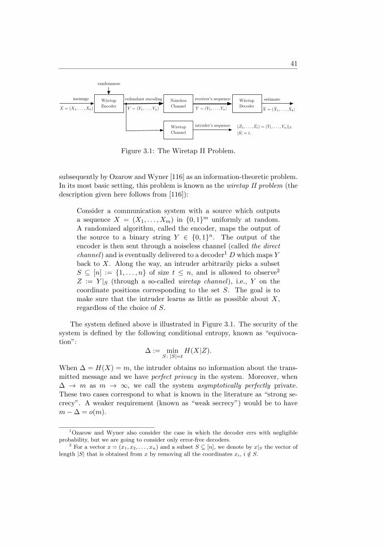
41
WiretapEncoder
X = (X1, . . . ,Xk) Y = (Y1, . . . , Yn)
Noiseless Channel
message redundant encoding receiver’s sequence
Y = (Y1, . . . , Yn)
Wiretap Decoder
estimate
X = (X1, . . . , Xk)
randomness
Wiretap Channel
intruder’s sequence (Z1, . . . , Zt) = (Y1, . . . , Yn)|S|S| = t.
Figure 3.1: The Wiretap II Problem.
subsequently by Ozarow and Wyner [116] as an information-theoretic problem.In its most basic setting, this problem is known as the wiretap II problem (thedescription given here follows from [116]):
Consider a communication system with a source which outputsa sequence X = (X1, . . . , Xm) in 0, 1m uniformly at random.A randomized algorithm, called the encoder, maps the output ofthe source to a binary string Y ∈ 0, 1n. The output of theencoder is then sent through a noiseless channel (called the directchannel) and is eventually delivered to a decoder1 D which maps Yback to X. Along the way, an intruder arbitrarily picks a subsetS ⊆ [n] := 1, . . . , n of size t ≤ n, and is allowed to observe2
Z := Y |S (through a so-called wiretap channel), i.e., Y on thecoordinate positions corresponding to the set S. The goal is tomake sure that the intruder learns as little as possible about X,regardless of the choice of S.
The system defined above is illustrated in Figure 3.1. The security of thesystem is defined by the following conditional entropy, known as “equivoca-tion”:
∆ := minS : |S|=t
H(X|Z).
When ∆ = H(X) = m, the intruder obtains no information about the trans-mitted message and we have perfect privacy in the system. Moreover, when∆ → m as m → ∞, we call the system asymptotically perfectly private.These two cases correspond to what is known in the literature as “strong se-crecy”. A weaker requirement (known as “weak secrecy”) would be to havem−∆ = o(m).
1Ozarow and Wyner also consider the case in which the decoder errs with negligibleprobability, but we are going to consider only error-free decoders.
2 For a vector x = (x1, x2, . . . , xn) and a subset S ⊆ [n], we denote by x|S the vector oflength |S| that is obtained from x by removing all the coordinates xi, i /∈ S.
42 CHAPTER 3. THE WIRETAP CHANNEL PROBLEM
Remark 3.1. The assumption that X is sampled from a uniformly randomsource should not be confused with the fact that Alice is transmitting oneparticular message to Bob that is fixed and known to her before the trans-mission. In this case, the randomness of X in the model captures the a prioriuncertainty about X for the outside world, and in particular the intruder, butnot the transmitter.
As an intuitive example, suppose that a random key is agreed upon be-tween Alice and a trusted third party, and now Alice wishes to securely sendher particular key to Bob over a wiretapped channel. Or, assume that Alicewishes to send an audio stream to Bob that is encoded and compressed usinga conventional audio encoding method.
Furthermore, the particular choice of the distribution on X as a uniformlyrandom sequence will cause no loss of generality. If the distribution of X ispublicly known to be non-uniform, the transmitter can use a suitable source-coding scheme to compress the source to its entropy prior to the transmission,and ensure that from the intruder’s point of view, X is uniformly distributed.On the other hand, it is also easy to see that if a protocol achieves perfectprivacy under uniform message distribution, it achieves perfect privacy underany other distribution as well.
3.1 The Formal Model
The model that we will be considering in this chapter is motivated by theoriginal wiretap channel problem but is more stringent in terms of its securityrequirements. In particular, instead of using Shannon entropy as a measure ofuncertainty, we will rely on statistical indistinguishability which is a strongermeasure that is more widely used in cryptography.
Definition 3.2. Let Σ be a set of size q, m and n be positive integers, andε, γ > 0. A (t, ε, γ)q-resilient wiretap protocol of block length n and messagelength m is a pair of functions E : Σm × 0, 1r → Σn (the encoder) andD : Σn → Σm (the decoder) that are computable in time polynomial in m,such that
(a) (Decodability) For all x ∈ Σm and all z ∈ 0, 1r we have D(E(x, z)) =x,
(b) (Resiliency) Let X ∼ UΣm , R ∼ Ur, and Y = E(X,R). For a set S ⊆ [n]and w ∈ Σ|S|, let XS,w denote the distribution of X conditioned on theevent Y |S = w. Define the set of bad observations as
BS := w ∈ Σ|S| | dist(XS,w,UΣm) > ε,where dist(·, ·) denotes the statistical distance between two distributions.Then we require that for every S ⊆ [n] of size at most t, Pr[Y |S ∈ BS ] ≤γ, where the probability is over the randomness of X and R.
3.1. THE FORMAL MODEL 43
The encoding of a vector x ∈ Σk is accomplished by choosing a vectorZ ∈ 0, 1r uniformly at random, and calculating E(x, Z). The quantitiesR := m/n, ε, and γ are called the rate, the error, and the leakage of theprotocol, respectively. Moreover, we call δ := t/n the (relative) resilience ofthe protocol.
The decodability condition ensures that the functions E and D are amatching encoder/decoder pair, while the resiliency conditions ensures thatthe intruder learns almost nothing about the message from his observation.
In our definition, the imperfection of the protocol is captured by the twoparameters ε and γ. When ε = γ = 0, the above definition coincides with theoriginal wiretap channel problem for the case of perfect privacy.
When γ = 0, we will have a worst-case guarantee, namely, that the in-truder’s views of the message before and after his observation are statisticallyclose, regardless of the outcome of the observation.
The protocol remains interesting even when γ is positive but sufficientlysmall. When γ > 0, a particular observation might potentially reveal to theintruder a lot of information about the message. However, a negligible γwill ensure that such a bad event (or leakage) happens only with negligibleprobability.
All the constructions that we will study in this chapter achieve zero leakage(i.e., γ = 0), except for the general result in Section 3.7.3 for which a nonzeroleakage is inevitable.
The significance of zero-leakage protocols is that they assure adaptive re-siliency in the weak sense introduced in [47] for exposure-resilient functions: ifthe intruder is given the encoded sequence as an oracle that he can adaptivelyquery at up to t coordinates (that is, the choice of each query may depend onthe outcome of the previous queries), and is afterwards presented with a chal-lenge which is either the original message or an independent uniformly chosenrandom string, he will not be able to distinguish between the two cases.
In general, it is straightforward to verify that our model can be used tosolve the original wiretap II problem, with ∆ ≥ m(1− ε− γ):
Lemma 3.3. Suppose that (E,D) is an encoder/decoder pair as in Defini-tion 3.2. Then using E and D in the wiretap II problem attains an equivoca-tion
∆ ≥ m(1− ε− γ).
Proof. Let W := Y |S be the intruder’s observation, and denote by W ′ the setof good observations, namely,
W ′ := w ∈ Σt : dist(XS,w,UΣm) ≤ ε.
44 CHAPTER 3. THE WIRETAP CHANNEL PROBLEM
Denote by H(·) the Shannon entropy in d-ary symbols. Then we will have
H(X|W ) =∑w∈Σt
Pr(W = w)H(X|W = w)
≥∑w∈W ′
Pr(W = w)H(X|W = w)
(a)
≥∑w∈W ′
Pr(W = w)(1− ε)m(b)
≥ (1− γ)(1− ε)m ≥ (1− γ − ε)m.
The inequality (a) follows from the definition of W ′ combined with Proposi-tion 3.30 in the appendix, and (b) by the definition of leakage parameter.
Hence, we will achieve asymptotically perfect privacy when ε+γ = o(1/m).For all the protocols that we present in this chapter this quantity will besuperpolynomially small; that is, smaller than 1/mc for every positive constantc (provided that m is large enough).
3.2 Review of the Related Notions inCryptography
There are several interrelated notions in the literature on Cryptography andTheoretical Computer Science that are also closely related to our definition ofthe wiretap protocol (Definition 3.2). These are resilient functions (RF) andalmost perfect resilient functions (APRF), exposure-resilient functions (ERF),and all-or-nothing transforms (AONT) (cf. [22,36,61,62,96,126,143] and [45]for a comprehensive account of several important results in this area).
The notion of resilient functions was introduced in [11] (and also [158]as the bit-extraction problem). A deterministic polynomial-time computablefunction f : 0, 1n → 0, 1m is called t-resilient if whenever any t bits ofthe its input are arbitrarily chosen by an adversary and the rest of the bitsare chosen uniformly at random, then the output distribution of the functionis (close to) uniform. APRF is a stronger variation where the criterion foruniformity of the output distribution is defined with respect to the `∞ (i.e.,point-wise distance of distributions) rather than `1. This stronger requirementallows for an “adaptive security” of APRFs.
ERFs, introduced in [22], are similar to resilient functions except that theentire input is chosen uniformly at random, and the view of the adversaryfrom the output remains (close to) uniform even after observing any t inputbits of his choice.
ERFs and resilient functions are known to be useful in a scenario similar tothe wiretap channel problem where the two parties aim to agree on any randomstring, for example a session key (Alice generates x uniformly at random whichshe sends to Bob, and then they agree on the string f(x)). Here no control
3.2. REVIEW OF THE RELATED NOTIONS IN CRYPTOGRAPHY 45
on the content of the message is required, and the only goal is that at the endof the protocol the two parties agree on any random string that is uniformeven conditioned on the observations of the intruder. Hence, Definition 3.2 ofa wiretap protocol is more stringent than that of resilient functions, since itrequires the existence and efficient computability of the encoding function Ethat provides a control over the content of the message.
Another closely related notion is that of all-or-nothing transforms, whichwas suggested in [126] for protection of block ciphers. A randomized poly-nomial-time computable function f : 0, 1m → 0, 1n, (m ≤ n), is called a(statistical, non-adaptive, and secret-only) t-AONT with error ε if it is effi-ciently invertible and for every S ⊆ [n] such that |S| ≤ t, and all x1, x2 ∈0, 1m we have that the two distributions f(x1)|S and f(x2)|S are ε-close.
An AONT with ε = 0 is called perfect. It is easy to see that perfectlyprivate wiretap protocols are equivalent to perfect adaptive AONTs. It wasshown in [47] that such functions can not exist (with positive, constant rate)when the adversary is allowed to observe more than half of the encoded bits.A similar result was obtained in [36] for the case of perfect linear RFs.
As pointed out in [47], AONTs can be used in the original scenario ofOzarow and Wyner’s wiretap channel problem. However, the best knownconstructions of AONTs can achieve rate-resilience trade-offs that are far fromthe information-theoretic optimum (see Figure 3.2).
While an AONT requires indistinguishability of intruder’s view for everyfixed pair (x1, x2) of messages, the relaxed notion of average-case AONT re-quires the expected distance of f(x1)|S and f(x2)|S to be at most ε for auniform random message pair. Hence, for a negligible ε, the distance will benegligible for all but a negligible fraction of message pairs. Up to a loss inparameters, wiretap protocols are equivalent to average case AONTs:
Lemma 3.4. Let (E,D) be an encoding/decoding pair for a (t, ε, γ)2-resilientwiretap protocol. Then E is an average-case t-AONT with error at most2(ε+ γ).
Conversely, an average-case t-AONT with error η2 can be used as a (t, η, η)-resilient wiretap encoder.
Proof. Consider a (t, ε, γ)2-resilient wiretap protocol as in Definition 3.2, andaccordingly, let the random variable Y = E(X,R) denote the encoding of Xwith a random seed R. For a set S ⊆ [n] of size at most t, denote by W := Y |Sthe intruder’s observation.
The resiliency condition implies that, the set of bad observations BS has aprobability mass of at most γ and hence, the expected distance dist(X|W,X)taken over the distribution of W is at most ε+ γ. Now we can apply Propo-sition 3.31 to the jointly distributed pair of random variables (W,X), andconclude that the expected distance dist(W |X,W ) over the distribution ofX (which is uniform) is at most ε + γ. This implies that the encoder is anaverage-case t-AONT with error at most 2(ε+ γ).
46 CHAPTER 3. THE WIRETAP CHANNEL PROBLEM
Conversely, the same argument combined with Markov’s bound shows thatan average-case t-AONT with error η2 can be seen as (t, η, η)-resilient wiretapprotocol.
Note that the converse direction does not guarantee zero leakage, andhence, zero leakage wiretap protocols are in general stronger than average-case AONTs. An average-case to worst-case reduction for AONTs was shownin [22] which, combined with the above lemma, can be used to show that anywiretap protocol can be used to construct an AONT (at the cost of a rateloss).
A simple universal transformation was proposed in [22] to obtain an AONTfrom any ERF, by one-time padding the message with a random string ob-tained from the ERF. In particular, given an ERF f : 0, 1n → 0, 1m,the AONT g : 0, 1m → 0, 1m+n is defined as g(x) := (r, x + f(r)), wherer ∈ 0, 1n is chosen uniformly at random. Hence, the ERF is used to one-timepad the message with a random secret string.
This construction can also yield a wiretap protocol with zero leakage. How-ever, it has the drawback of significantly weakening the rate-resilience trade-off. Namely, even if an information theoretically optimal ERF is used in thisreduction, the resulting wiretap protocol will only achieve half the optimalrate (see Figure 3.2). This is because the one-time padding strategy necessar-ily requires a random seed that is at least as long as the message itself, evenif the intruder is restricted to observe only a small fraction of the transmittedsequence. Hence the rate of the resulting AONT cannot exceed 1/2, and it isnot clear how to improve this universal transformation to obtain a worst-caseAONT using a shorter seed.
The main focus of this chapter is on asymptotic trade-offs between the rateR and the resilience δ of an asymptotically perfectly private wiretap protocol.For applications in cryptography, e.g., the context of ERFs or AONTs, it istypically assumed that the adversary learns all but a small number of thebits in the encoded sequence, and the incurred blow-up in the encoding is notas crucially important, as long as it remains within a reasonable range. Onthe other hand, as in this chapter we are motivated by the wiretap channelproblem which is a communication problem, optimizing the transmission ratewill be the most important concern for us. We will focus on the case wherethe fraction δ of the symbols observed by the intruder is an arbitrary constantbelow 1, which is the most interesting range in our context. However, someof our constructions work for sub-constant 1− δ as well.
Following [116], it is easy to see that, for resilience δ, an information-theoretic bound R ≤ 1− δ + o(1) must hold. Lower bounds for R in terms ofδ have been studied by a number of researchers.
For the case of perfect privacy (where the equivocation ∆ is equal to themessage length m), Ozarow and Wyner [116] give a construction of a wiretapprotocol using linear error-correcting codes, and show that the existence of an
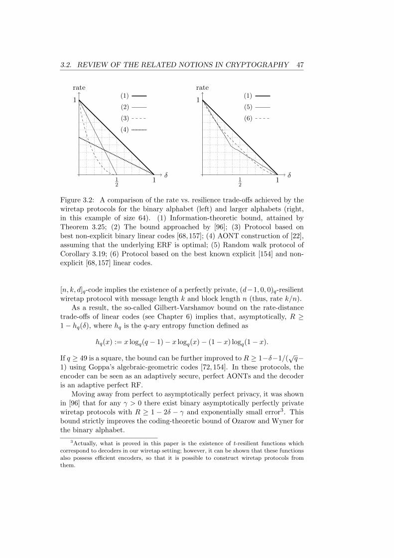
3.2. REVIEW OF THE RELATED NOTIONS IN CRYPTOGRAPHY 47
δ
rate
1
112
(1)
(2)
(3)
(4)
12
δ
rate
1
1
(1)
(5)
(6)
Figure 3.2: A comparison of the rate vs. resilience trade-offs achieved by thewiretap protocols for the binary alphabet (left) and larger alphabets (right,in this example of size 64). (1) Information-theoretic bound, attained byTheorem 3.25; (2) The bound approached by [96]; (3) Protocol based onbest non-explicit binary linear codes [68,157]; (4) AONT construction of [22],assuming that the underlying ERF is optimal; (5) Random walk protocol ofCorollary 3.19; (6) Protocol based on the best known explicit [154] and non-explicit [68, 157] linear codes.
[n, k, d]q-code implies the existence of a perfectly private, (d−1, 0, 0)q-resilientwiretap protocol with message length k and block length n (thus, rate k/n).
As a result, the so-called Gilbert-Varshamov bound on the rate-distancetrade-offs of linear codes (see Chapter 6) implies that, asymptotically, R ≥1− hq(δ), where hq is the q-ary entropy function defined as
hq(x) := x logq(q − 1)− x logq(x)− (1− x) logq(1− x).
If q ≥ 49 is a square, the bound can be further improved to R ≥ 1−δ−1/(√q−
1) using Goppa’s algebraic-geometric codes [72, 154]. In these protocols, theencoder can be seen as an adaptively secure, perfect AONTs and the decoderis an adaptive perfect RF.
Moving away from perfect to asymptotically perfect privacy, it was shownin [96] that for any γ > 0 there exist binary asymptotically perfectly privatewiretap protocols with R ≥ 1 − 2δ − γ and exponentially small error3. Thisbound strictly improves the coding-theoretic bound of Ozarow and Wyner forthe binary alphabet.
3Actually, what is proved in this paper is the existence of t-resilient functions whichcorrespond to decoders in our wiretap setting; however, it can be shown that these functionsalso possess efficient encoders, so that it is possible to construct wiretap protocols fromthem.
48 CHAPTER 3. THE WIRETAP CHANNEL PROBLEM
3.3 Symbol-Fixing and Affine Extractors
Two central notions for our constructions of wiretap protocols in this chapterare symbol-fixing and affine extractors. In this section, we introduce thesenotions, and study some basic constructions.
Definition 3.5. A d-ary symbol-fixing source is an imperfect source of randomsymbols from an alphabet of size d, that may fix some bounded number of thesymbols to unknown values. More precisely, an (n, k)d symbol-fixing source isthe distribution of a random variable X = (X1, X2, . . . , Xn) ∈ Σn, for someset Σ of size d, in which at least k of the coordinates (chosen arbitrarily) areuniformly and independently distributed on Σ and the rest take deterministicvalues.
When d = 2, we will have a binary symbol-fixing source, or simply a bit-fixing source. In this case Σ = 0, 1, and the subscript d is dropped from thenotation.
The min-entropy of a (n, k)d symbol-fixing source is k log2 d bits. For ad-ary source with d 6= 2, it is more convenient to talk about the d-ary entropyof the source, which is k (in d-ary symbols).
Affine sources are natural generalizations of symbol-fixing sources whenthe alphabet size is a prime power.
Definition 3.6. For a prime power q, an (n, k)q affine source is a distri-bution on Fnq that is uniformly supported on an affine translation of somek-dimensional subspace of Fnq .
It is easy to see that the q-ary min-entropy of a k-dimensional affine sourceis k. Due to the restricted structure of symbol-fixing and affine sources, it ispossible to construct seedless extractors for such sources:
Definition 3.7. Let Σ be a finite alphabet of size d > 1. A function f : Σn →Σm is a (seedless) (k, ε)-extractor for symbol-fixing (resp., affine) sources on Σn
if for every (n, k)d symbol-fixing (resp., affine) source X , the distribution E(X )is ε-close to the uniform distribution UΣm . The extractor is called explicit ifit is deterministic and polynomial-time computable.
We will shortly see simple constructions of zero-error, symbol-fixing andaffine extractors using linear functions arising from good error-correcting codes.These extractors achieve the lowest possible error, but however are unable toextract the entire source entropy. Moreover, the affine extractor only works fora “restricted” class of affine sources. For unrestricted affine sources, there areby now various constructions of extractors in the literature. Here we reviewsome notable examples that are most useful for the construction of wiretapprotocols that we will discuss in this chapter.
Over large fields, the following affine extractor due to Gabizon and Razextract almost the entire source entropy:
3.3. SYMBOL-FIXING AND AFFINE EXTRACTORS 49
Theorem 3.8. [65] There is a constant q0 such that for any prime power fieldsize q and integers n, k such that q > maxq0, n
20, there is an explicit affine(k, ε)-extractor f : Fnq → Fk−1
q , where ε < q−1/21.
In this construction, the field size has to be polynomially large in n. Whenthe field size is small (in particular, constant), the task becomes much morechallenging. The most challenging case thus corresponds to the binary fieldF2, for which an explicit affine extractor was obtained, when the input entropyis a constant fraction of the input length, by Bourgain:
Theorem 3.9. [16] For every constant 0 < δ ≤ 1, there is an explicit affineextractor AExt : Fn2 → Fm2 for min-entropy δn with output length m = Ω(n)and error at most 2−Ω(m).
Bourgain’s construction was recently simplified, improved, and extendedto work for arbitrary prime fields by Yehudayoff [167].
An “intermediate” trade-off is recently obtained by DeVos and Gabizon[44], albeit with a short output length. This explicit construction extracts oneunbiased bit from any (n, k)q affine source provided that, for d := 5n/k, wehave q > 2d2 and the characteristic of the field is larger than d.
3.3.1 Symbol-Fixing Extractors from Linear Codes
The simple theorem below states that linear error-correcting codes can be usedto obtain symbol-fixing extractors with zero error.
Theorem 3.10. Let C be an [n, k, d]q code over Fq and G be a k×n generator
matrix of C. Then, the function E : Fnq → Fkq defined as4 E(x) := Gx> is an(n− d+ 1, 0)-extractor for symbol-fixing sources over Fq.
Conversely, if a linear function E : Fnq → Fkq is an (n− d+ 1, 0)-extractorfor symbol-fixing sources over Fq, it corresponds to a generator matrix of an[n, k, d]q code.
Proof. Let X be a symbol-fixing source with a set S ⊆ [n] of fixed coordinates,where5 |S| = d − 1, and define S := [n] \ S. Observe that, by the Singletonbound, we must have |S| = n− d+ 1 ≥ k.
The submatrix of G obtained by removing the columns picked by S musthave rank k. Since otherwise, the left kernel of this submatrix would benonzero, meaning that C has a nonzero codeword that consists of entirelyzeros at the d−1 positions picked by S, contradicting the assumption that theminimum distance of C is d. Therefore, the distribution E(X ) is supported on
a k-dimensional affine space on Fkq , meaning that this distribution is uniform.
4We typically consider vectors be represented in row form, and use the transpose operator(x>) to represent column vectors.
5If the set of fixed symbols if of size smaller than d− 1, the argument still goes throughby taking S as an arbitrary set of size d− 1 containing all the fixed coordinates.
50 CHAPTER 3. THE WIRETAP CHANNEL PROBLEM
The converse is straightforward by following the same argument.
If the field size is large enough; e.g., q ≥ n, then one can pick C in the abovetheorem to be an MDS code (in particular, a Reed-Solomon code) to obtain a(k, 0)-extractor for all symbol-fixing sources of entropy k with optimal outputlength k. However, for a fixed q, negative results on the rate-distance trade-offs of codes (e.g., Hamming, MRRW, and Plotkin bounds) assert that thisconstruction of extractors must inevitably lose some fraction of the entropy ofthe source. Moreover, the construction would at best be able to extract someconstant fraction of the source entropy only if the entropy of the source (inq-ary symbols) is above n/q.
3.3.2 Restricted Affine Extractors from Rank-Metric Codes
In Section 3.7, we will see that affine extractors can be used to constructwiretap schemes for models that are more general than the original Wiretap IIproblem, e.g., when the direct channel is noisy. For these applications, theextractor needs to additionally have a nice structure that is in particularoffered by linear functions.
An obvious observation is that a nontrivial affine extractor cannot be alinear function. Indeed, a linear function f(x) := 〈α, x〉 + β, where α, β, x ∈Fnq , is constant on the (n−1)-dimensional orthogonal subspace of α, and thus,fails to be an extractor for even (n − 1)-dimensional affine spaces. However,in this section we will see that linear affine extractors can be constructed ifthe affine source is known to be described by a set of linear constraints whosecoefficients lie on a small sub-field of the underlying field. Such restrictedextractors turn out to be sufficient for some of the applications that we willconsider.
Let Q be a prime power. Same as linear codes, an affine subspace onFnQ can be represented by a generator matrix, or parity-check matrix anda constant shift. That is, a k-dimensional affine subspace A ⊆ FnQ can bedescribed as the image of a linear mapping
A := xG+ β : x ∈ FkQ,
where G is a k × n generator matrix of rank k over FQ, and β ∈ FnQ is afixed vector. Alternatively, A can be expressed as the translated null-space ofa linear mapping
A := x+ β ∈ FnQ : Hx> = 0,for an (n− k)× n parity check matrix of rank n− k over FQ.
Observe that a symbol-fixing source over Fq with q-ary min-entropy k canbe seen as a k-dimensional affine source with a generator matrix of the form[I | 0] · P , where I is the k × k identity matrix, 0 denotes the k × (n− k) all-zeros matrix, and P is a permutation matrix. Recall that from Theorem 3.10
3.3. SYMBOL-FIXING AND AFFINE EXTRACTORS 51
we know that for this restricted type of affine sources linear extractors exist.In this section we generalize this idea.
Suppose that Q = qm for a prime power q so that FQ can be regardedas a degree m extension of Fq (and isomorphic to Fqm). Let A be an affinesource over FnQ. We will call the affine source Fq-restricted if its support canbe represented by a generator matrix (or equivalently, a parity check matrix)over Fq.
In this section we introduce an affine extractor that is FQ-linear and,assuming that m is sufficiently large, extracts from Fq-restricted affine sources.The construction of the extractor is similar to Theorem 3.10, except thatinstead of an error-correcting code defined over the Hamming metric, we willuse rank-metric codes.
Consider the function rdist : Fm×nq ×Fm×nq → Z, where Fm×nq denotes theset of m× n matrices over Fq, defined as rdist(A,B) := rankq(A− B), whererankq is the matrix rank over Fq. It is straightforward to see that rdist is ametric.
The usual notion of error-correcting codes defined under the Hammingmetric can be naturally extended to the rank metric. In particular, a rank-metric code C can be defined as a set of m×n matrices (known as codewords),whose minimum distance is the minimum rank distance between pairs of code-words.
ForQ := qm, there is a natural correspondence betweenm×nmatrices overFq and vectors of length n over FQ. Consider an isomorphism ϕ : FQ → Fmqbetween FQ and Fmq which maps elements of FQ to column vectors of lengthm over Fq. Then one can define a mapping Φ: FnQ → Fm×nq defined as
Φ(x1, . . . , xn) := [ϕ(x1) | · · · | ϕ(xn)]
to put the elements of FnQ in one-to-one correspondence with m× n matricesover Fq.
A particular class of rank-metric codes are linear ones. Suppose that Cis a linear [n, k, d]Q code over FQ. Then, using Φ(·), C can be regarded as arank-metric code of dimension k over Fm×nq . In symbols, we will denote such
a linear k-dimensional rank-metric code as an [[n, k, d]]qm code, where d is theminimum rank-distance of the code. The rank-distance of a linear rank-metriccode turns out to be equal to the minimum rank of its nonzero codewords andobviously, one must have d ≤ d. However, the Hamming distance of C mightturn out to be much larger than its rank distance when regarded as a rank-metric code. In particular, d ≤ m, and thus, d must be strictly smaller thand when the degree m of the field extension is less than d.
A counterpart of the Singleton bound in the rank-metric states that, forany [[n, k, d]]qm code, one must have d ≤ n − k + 1. Rank-metric codes thatattain equality exist and are called maximum rank distance (MRD) codes.A class of linear rank-metric codes known as Gabidulin codes [64] are MRD
52 CHAPTER 3. THE WIRETAP CHANNEL PROBLEM
and can be thought of as the counterpart of Reed-Solomon codes in the rankmetric. In particular, the codewords of a Gabidulin code, seen as vectorsover the extension field, are evaluation vectors of bounded-degree linearizedpolynomials rather than arbitrary polynomials as in the case of Reed-Solomoncodes. These codes are defined for any choice of n, k, q,m as long as m ≥ nand k ≤ n.
The following is an extension of Theorem 3.10 to restricted affine sources.
Theorem 3.11. Let C be an [[n, k, d]]qm code defined from a code over FQ
(where Q := qm) with a generator matrix G ∈ Fk×nQ . Then the function
E : FnQ → FkQ defined as E(x) := Gx> is an (n − d + 1, 0)-extractor for Fq-restricted affine sources over FQ.
Conversely, if a linear function E : FnQ → FkQ is an (n−d+1, 0)-extractor forall Fq-restricted affine sources over FQ, it corresponds to a generator matrixof an [[n, k, d]]qm code.
Proof. Consider a restricted affine source X uniformly supported on an affinesubspace of dimension6 n− d+ 1
X := xA+ β : x ∈ Fn−d+1Q ,
where A ∈ F(n−d+1)×nq has rank n− d+ 1, and β ∈ FnQ is a fixed translation.
Note that k ≤ n− d+ 1 by the Singleton bound for rank-metric codes.The output of the extractor is thus uniformly supported on the affine
subspace
B := GA>x> +Gβ> : x ∈ Fn−d+1Q ⊆ FkQ.
Note that GA> ∈ Fk×(n−d+1)Q . Our goal is to show that the dimension
of B is equal to k. Suppose not, then we must have rankQ(GA>) < k. In
particular, there is a nonzero y ∈ FkQ such that yGA> = 0.
Let Y := Φ(yG) ∈ Fm×nq , where Φ(·) is the isomorphism that maps code-words of C to their matrix form over Fq. By the distance of C, we know thatrankq(Y ) ≥ d. Since m ≥ d, this means that Y has at least d linearly indepen-
dent rows. On the other hand, we know that the matrix Y A> ∈ Fk×(n−d+1)q
is the zero matrix. Therefore, Y has d independent rows (each in Fnq ) that areall orthogonal to the n−d+1 independent rows of A. Since d+(n−d+1) > n,this is a contradiction.
Therefore, the dimension of B is exactly k, meaning that the output dis-tribution of the extractor is indeed uniform. The converse is straightforwardby following a similar line of argument.
6 The argument still holds if the dimension of X is more than n− d+ 1.
3.4. INVERTING EXTRACTORS 53
Thus, in particular, we see that generator matrices of MRD codes can beused to construct linear extractors for restricted affine sources that extractthe entire source entropy with zero error. This is possible provided that thefield size is large enough compared to the field size required to describe thegenerator matrix of the affine source. Using Gabidulin’s rank metric codes,we immediately obtain the following corollary of Theorem 3.11:
Corollary 3.12. Let q be a prime power. Then for every positive integern, k ≤ n, and Q := qn, there is a linear function f : FnQ → FkQ that is a(k, 0)-extractor for Fq-restricted affine sources over FQ.
It can be shown using similar proofs that if, in Theorems 3.10 and 3.11,a parity check matrix of the code is used instead of a generator matrix, theresulting linear function would become a lossless (d − 1, 0)-condenser ratherthan an extractor. This is in fact part of a more general “duality” phenomenonthat is discussed in Section 5.5.
3.4 Inverting Extractors
In this section we will introduce the notion of invertible extractors and its con-nection with wiretap protocols7. Later we will use this connection to constructwiretap protocols with good rate-resilience trade-offs.
Definition 3.13. Let Σ be a finite alphabet and f be a mapping from Σn toΣm. For γ ≥ 0, a function A : Σm × 0, 1r → Σn is called a γ-inverter for fif the following conditions hold:
(a) (Inversion) Given x ∈ Σm such that f−1(x) is nonempty, for every z ∈0, 1r we have f(A(x, z)) = x.
(b) (Uniformity) A(UΣm ,Ur) ∼γ UΣn .
A γ-inverter is called efficient if there is a randomized algorithm that runsin worst case polynomial time and, given x ∈ Σm and z as a random seed,computes A(x, z). We call a mapping γ-invertible if it has an efficient γ-inverter, and drop the prefix γ from the notation when it is zero.
The parameter r in the above definition captures the amount of randombits that the inverter (seen as a randomized algorithm) needs to receive. For
7 Another notion of invertible extractors was introduced in [46] and used in [48] fora different application (entropic security) that should not be confused with the one weuse. Their notion applies to seeded extractors with long seeds that are efficiently invertiblebijections for every fixed seed. Such extractors can be seen as a single-step walk on highlyexpanding graphs that mix in one step. This is in a way similar to the multiple-step randomwalk used in the seedless extractor of section 3.5, that can be regarded as a single-step walkon the expander graph raised to a certain power.
54 CHAPTER 3. THE WIRETAP CHANNEL PROBLEM
our applications, no particular care is needed to optimize this parameter and,as long as r is polynomially bounded in n, it is generally ignored.
Remark 3.14. If a function f maps the uniform distribution to a distribu-tion that is ε-close to uniform (as is the case for all extractors), then anyrandomized mapping that maps its input x to a distribution that is γ-close tothe uniform distribution on f−1(x) is easily seen to be an (ε+ γ)-inverter forf . In some situations designing such a function might be easier than directlyfollowing the above definition.
The idea of random pre-image sampling was proposed in [47] for construc-tion of adaptive AONTs from APRFs. However, they ignored the efficiencyof the inversion, as their goal was to show the existence of (not necessarilyefficient) information-theoretically optimal adaptive AONTs. Moreover, thestrong notion of APRF and a perfectly uniform sampler is necessary for theirconstruction of AONTs. As wiretap protocols are weaker than (worst-case)AONTs, they can be constructed from slightly imperfect inverters as shownby the following lemma.
Lemma 3.15. Let Σ be an alphabet of size q > 1 and f : Σn → Σm be a(γ2/2)-invertible q-ary (k, ε) symbol-fixing extractor. Then, f and its invertercan be seen as a decoder/encoder pair for an (n−k, ε+γ, γ)q-resilient wiretapprotocol with block length n and message length m.
Proof. Let E and D denote the wiretap encoder and decoder, respectively.Hence, E is the (γ2/2)-inverter for f , and D is the extractor f itself. Fromthe definition of the inverter, for every x ∈ Σm and every random seed r, wehave D(E(x, r)) = x. Hence it is sufficient to show that the pair satisfies theresiliency condition.
Let the random variable X be uniformly distributed on Σm and the seedR ∈ 0, 1r be chosen uniformly at random. Denote the encoding of X byY := E(X,R). Fix any S ⊆ [n] of size at most n− k.
For every w ∈ Σ|S|, let Yw denote the set y ∈ Σn : (y|S) = w. Note thatthe sets Yw partition the space Σn into |Σ||S| disjoint sets.
Let Y and YS denote the distribution of Y and Y |S , respectively. Theinverter guarantees that Y is (γ2/2)-close to uniform. Applying Proposi-tion 3.32, we get that∑
w∈Σ|S|
Pr[(Y |S) = w] · dist((Y|Yw),UYw) ≤ γ2.
The left hand side is the expectation of dist((Y|Yw),UYw). Denote by W theset of all bad outcomes of Y |S , i.e.,
W := w ∈ Σ|S| | dist((Y|Yw),UYw) > γ.
3.5. A WIRETAP PROTOCOL BASED ON RANDOM WALKS 55
By Markov’s inequality, we conclude that
Pr[(Y |S) ∈W ] ≤ γ.
For every w ∈ W , the distribution of Y conditioned on the event (Y |S) = wis γ-close to a symbol-fixing source with n − |S| ≥ k random symbols. Thefact that D is a symbol-fixing extractor for this entropy and Proposition 3.33imply that, for any such w, the conditional distribution of D(Y )|(Y |S = w) is(γ+ ε)-close to uniform. Hence with probability at least 1−γ the distributionof X conditioned on the outcome of Y |S is (γ + ε)-close to uniform. Thisensures the resiliency of the protocol.
By combining Lemma 3.15 and Theorem 3.10 using a Reed-Solomon code,we can obtain a perfectly private, rate-optimal, wiretap protocol for the Wire-tap II problem over large alphabets (namely, q ≥ n), and recover the originalresult of Ozarow and Wyner8 [116]:
Corollary 3.16. For every positive integer n, prime power q ≥ n, and δ ∈[0, 1), there is a (δn, 0, 0)q-resilient wiretap protocol with block length n andrate 1− δ that attains perfect privacy.
3.5 A Wiretap Protocol Based on Random Walks
In this section we describe a wiretap protocol that achieves a rate R withina constant fraction of the information theoretically optimal value 1 − δ (theconstant depending on the alphabet size).
To achieve our result, we will modify the symbol-fixing extractor of Kampand Zuckerman [88], that is based on random walks on expander graphs, tomake it efficiently invertible without affecting its extraction properties, andthen apply Lemma 3.15 above to obtain the desired wiretap protocol.
Before we proceed, let us briefly review some basic notions and facts relatedto expander graphs. For a detailed review of the theory of expander graphs,refer to the excellent survey by Hoory, Linial and Wigderson [82], and books[109,112].
We will be working with directed regular expander graphs that are ob-tained from undirected graphs by replacing each undirected edge with twodirected edges in opposite directions. Let G = (V,E) be a d-regular graph.Then a labeling of the edges of G is a function L : V × [d]→ V such that forevery u ∈ V and t ∈ [d], the edge (u, L(u, t)) is in E. The labeling is consistentif whenever L(u, t) = L(v, t), then u = v. Note that the natural labeling of aCayley graph (cf. [82]) is in fact consistent.
A family of d-regular graphs is an infinite set of d-regular graphs such thatfor every N ∈ N, the set contains a graph with at least N vertices. For a
8In fact, Ozarow and Wyner use a parity check matrix of an MDS code in their con-struction, which is indeed a generator matrix for the dual code which is itself MDS.
56 CHAPTER 3. THE WIRETAP CHANNEL PROBLEM
parameter c ≥ 1, we will call a family c-dense if there is an N0 ∈ N such that,for every N ≥ N0, the family has a graph with at least N and at most cNvertices. We call a family of graphs constructible if all the graphs in the familyhave a consistent labeling that is efficiently computable. That is, there is auniform, polynomial-time algorithm that, given N ∈ N and i ∈ [N ], j ∈ [d],outputs the label of the jth neighbor of the ith vertex, under a consistentlabeling, in the graph in the family that has N vertices (provided that itexists).
Let A denote the normalized adjacency matrix of a d-regular graph G(that is, the adjacency matrix with all the entries divided by d). We denoteby λG the second largest eigenvalue of A in absolute value. The spectralgap of G is given by 1 − λG. Starting from a probability distribution p onthe set of vertices, represented as a real vector with coordinates index by thevertex set, performing a single-step random walk on G leads to the distributiondefined by pA. The following is a well known lemma on the convergence ofthe distributions resulting from random walks (see [99] for a proof):
Lemma 3.17. Let G = (V,E) be a d-regular undirected graph, and A be itsnormalized adjacency matrix. Then for any probability vector p, we have
‖pA− UV ‖2 ≤ λG‖p− UV ‖2,
where ‖ · ‖2 denotes the `2 norm.
The extractor of Kamp and Zuckerman [88] starts with a fixed vertex ina large expander graph and interprets the input as the description of a walkon the graph. Then it outputs the label of the vertex reached at the end ofthe walk. Notice that a direct approach to invert this function will amount tosampling a path of a particular length between a pair of vertices in the graph,uniformly among all the possibilities, which might be a difficult problem forgood families of expander graphs9. We work around this problem by choosingthe starting point of the walk from the input10. The price that we pay by doingso is a slightly larger error compared to the original construction of Kamp andZuckerman that is, asymptotically, of little significance. In particular we showthe following:
Theorem 3.18. Let G be a constructible d-regular graph with dm vertices andsecond largest eigenvalue λG ≥ 1/
√d. Then there exists an explicit invertible
9In fact intractability of the easier problem of finding a loop in certain families of ex-pander graphs forms the underlying basis for a class of cryptographic hash functions (cf.[25]). Even though this easier problem has been solved in [151], uniform sampling of pathsseems to be much more difficult.
10 The idea of choosing the starting point of the walk from the input sequence has beenused before in extractor constructions [172], but in the context of seeded extractors forgeneral sources with high entropy.
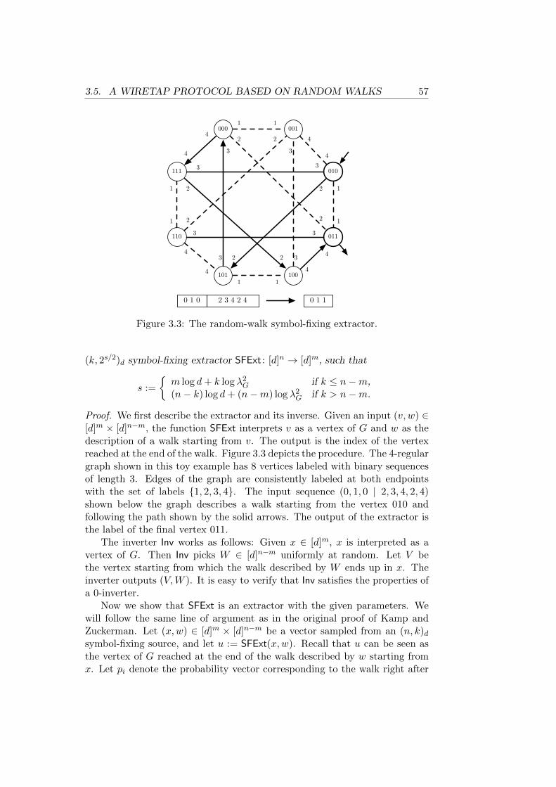
3.5. A WIRETAP PROTOCOL BASED ON RANDOM WALKS 57
000 001
111 010
110 011
101 100
1
2
3
41
2
3
4
4
3
21
1 2
3
4
4
3 2
1 1
4
2 3
3
4
12
43
12
2 3 4 2 40 1 0 0 1 1
Figure 3.3: The random-walk symbol-fixing extractor.
(k, 2s/2)d symbol-fixing extractor SFExt : [d]n → [d]m, such that
s :=
m log d+ k log λ2
G if k ≤ n−m,(n− k) log d+ (n−m) log λ2
G if k > n−m.
Proof. We first describe the extractor and its inverse. Given an input (v, w) ∈[d]m × [d]n−m, the function SFExt interprets v as a vertex of G and w as thedescription of a walk starting from v. The output is the index of the vertexreached at the end of the walk. Figure 3.3 depicts the procedure. The 4-regulargraph shown in this toy example has 8 vertices labeled with binary sequencesof length 3. Edges of the graph are consistently labeled at both endpointswith the set of labels 1, 2, 3, 4. The input sequence (0, 1, 0 | 2, 3, 4, 2, 4)shown below the graph describes a walk starting from the vertex 010 andfollowing the path shown by the solid arrows. The output of the extractor isthe label of the final vertex 011.
The inverter Inv works as follows: Given x ∈ [d]m, x is interpreted as avertex of G. Then Inv picks W ∈ [d]n−m uniformly at random. Let V bethe vertex starting from which the walk described by W ends up in x. Theinverter outputs (V,W ). It is easy to verify that Inv satisfies the properties ofa 0-inverter.
Now we show that SFExt is an extractor with the given parameters. Wewill follow the same line of argument as in the original proof of Kamp andZuckerman. Let (x,w) ∈ [d]m × [d]n−m be a vector sampled from an (n, k)dsymbol-fixing source, and let u := SFExt(x,w). Recall that u can be seen asthe vertex of G reached at the end of the walk described by w starting fromx. Let pi denote the probability vector corresponding to the walk right after
58 CHAPTER 3. THE WIRETAP CHANNEL PROBLEM
the ith step, for i = 0, . . . , n − m, and denote by p the uniform probabilityvector on the vertices of G. Our goal is to bound the error ε of the extractor,which is half the `1 norm of pn−m − p.
Suppose that x contains k1 random symbols and the remaining k2 := k−k1
random symbols are in w. Then p0 has the value d−k1 at dk1 of the coordinatesand zeros elsewhere, hence
‖p0 − p‖22 = dk1(d−k1 − d−m)2 + (dm − dk1)d−2m = d−k1 − d−m ≤ d−k1 .
Now for each i ∈ [n − m], if the ith step of the walk corresponds to arandom symbol in w the `2 distance is multiplied by λG by Lemma 3.17.Otherwise the distance remains the same due to the fact that the labeling ofG is consistent. Hence we obtain ‖pn−m − p‖22 ≤ d−k1λ2k2
G . Translating thisinto the `1 norm by using the Cauchy-Schwarz inequality, we obtain ε, namely,
ε ≤ 1
2d(m−k1)/2λk2
G < 2((m−k1) log d+k2 log λ2G)/2.
By our assumption, λG ≥ 1/√d. Hence, everything but k1 and k2 being fixed,
the above bound is maximized when k1 is minimized. When k ≤ n−m, thiscorresponds to the case k1 = 0, and otherwise to the case k1 = k − n + m.This gives us the desired upper bound on ε.
Combining this with Lemma 3.15 and setting up the the right asymptoticparameters, we obtain our protocol for the wiretap channel problem.
Corollary 3.19. Let δ ∈ [0, 1) and γ > 0 be arbitrary constants, and supposethat there is a constructible family of d-regular expander graphs with spectralgap at least 1− λ that is c-dense, for constants λ < 1 and c ≥ 1.
Then, for every large enough n, there is a (δn, 2−Ω(n), 0)d-resilient wiretapprotocol with block length n and rate
R = maxα(1− δ), 1− δ/α − γ,
where α := − logd λ2.
Proof. For the case c = 1 we use Lemma 3.15 with the extractor SFExt ofTheorem 3.18 and its inverse. Every infinite family of graphs must satisfyλ ≥ 2
√d− 1/d [114], and in particular we have λ ≥ 1/
√d, as required by
Theorem 3.18. We choose the parameters k := (1−δ)n and m := n(maxα(1−δ), 1 − δ/α − γ), which gives s = −Ω(n), and hence, exponentially smallerror. The case c > 1 is similar, but involves technicalities for dealing withlack of graphs of arbitrary size in the family. We will elaborate on this inAppendix 3.A.
Using explicit constructions of Ramanujan graphs that achieve
λ ≤ 2√d− 1/d
3.6. INVERTIBLE AFFINE EXTRACTORS 59
when d − 1 is a prime power [100, 110, 119], one can obtain α ≥ 1 − 2/ log d,which can be made arbitrarily close to one (hence, making the protocol arbi-trarily close to the optimal bound) by choosing a suitable alphabet size thatdoes not depend on n. Namely, we have the following result:
Corollary 3.20. Let δ ∈ [0, 1) and γ > 0 be arbitrary constants. Then, thereis a positive integer d only depending on γ such that the following holds: Forevery large enough n, there is a (δn, 2−Ω(n), 0)d-resilient wiretap protocol withblock length n and rate at least 1− δ − γ.
3.6 Invertible Affine Extractors andAsymptotically Optimal Wiretap Protocols
In this section we will construct a black box transformation for making certainseedless extractors invertible. The method is described in detail for affineextractors, and leads to wiretap protocols with asymptotically optimal rate-resilience trade-offs. Being based on affine extractors, these protocols are onlydefined for prime power alphabet sizes. On the other hand, the random-walk based protocol discussed in Section 3.5 can be potentially instantiatedfor an arbitrary alphabet size, though achieving asymptotically sub-optimalparameters (and a positive rate only for an alphabet of size 3 or more).
Modulo some minor differences, the construction can be simply describedas follows: A seedless affine extractor is first used to extract a small numberof uniform random bits from the source, and the resulting sequence is thenused as the seed for a seeded extractor that extracts almost the entire entropyof the source.
Of course, seeded extractors in general are not guaranteed to work if (asin the above construction) their seed is not independent from the source.However, as observed by Gabizon and Raz [65], a linear seeded extractor canextract from an affine source if the seed is the outcome of an affine extractor onthe source. This idea was formalized in a more general setting by Shaltiel [132].
Shaltiel’s result gives a general framework for transforming any seedlessextractor (for a family of sources satisfying a certain closedness condition)with short output length to one with an almost optimal output length. Theconstruction uses the imperfect seedless extractor to extract a small number ofuniform random bits from the source, and will then use the resulting sequenceas the seed for a seeded extractor to extract more random bits from the source.For a suitable choice of the seeded extractor, one can use this construction toextract almost all min-entropy of the source.
The closedness condition needed for this result to work for a family Cof sources is that, letting E(x, s) denote the seeded extractor with seed s, forevery X ∈ C and every fixed s and y, the distribution (X|E(X , s) = y) belongsto C. If E is a linear function for every fixed s, the result will be available for
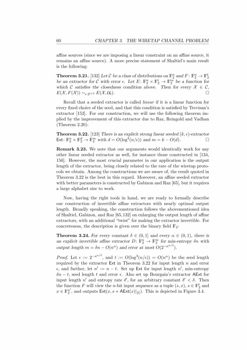
60 CHAPTER 3. THE WIRETAP CHANNEL PROBLEM
affine sources (since we are imposing a linear constraint on an affine source, itremains an affine source). A more precise statement of Shaltiel’s main resultis the following:
Theorem 3.21. [132] Let C be a class of distributions on Fn2 and F : Fn2 → Ft2be an extractor for C with error ε. Let E : Fn2 × Ft2 → Fm2 be a function forwhich C satisfies the closedness condition above. Then for every X ∈ C,E(X , F (X )) ∼ε·2t+3 E(X ,Ut).
Recall that a seeded extractor is called linear if it is a linear function forevery fixed choice of the seed, and that this condition is satisfied by Trevisan’sextractor [152]. For our construction, we will use the following theorem im-plied by the improvement of this extractor due to Raz, Reingold and Vadhan(Theorem 2.20):
Theorem 3.22. [123] There is an explicit strong linear seeded (k, ε)-extractorExt : Fn2 × Fd2 → Fm2 with d = O(log3(n/ε)) and m = k −O(d).
Remark 3.23. We note that our arguments would identically work for anyother linear seeded extractor as well, for instance those constructed in [134,150]. However, the most crucial parameter in our application is the outputlength of the extractor, being closely related to the rate of the wiretap proto-cols we obtain. Among the constructions we are aware of, the result quoted inTheorem 3.22 is the best in this regard. Moreover, an affine seeded extractorwith better parameters is constructed by Gabizon and Raz [65], but it requiresa large alphabet size to work.
Now, having the right tools in hand, we are ready to formally describeour construction of invertible affine extractors with nearly optimal outputlength. Broadly speaking, the construction follows the abovementioned ideaof Shaltiel, Gabizon, and Raz [65,132] on enlarging the output length of affineextractors, with an additional “twist” for making the extractor invertible. Forconcreteness, the description is given over the binary field F2:
Theorem 3.24. For every constant δ ∈ (0, 1] and every α ∈ (0, 1), there isan explicit invertible affine extractor D : Fn2 → Fm2 for min-entropy δn with
output length m = δn−O(nα) and error at most O(2−nα/3
).
Proof. Let ε := 2−nα/3
, and t := O(log3(n/ε)) = O(nα) be the seed lengthrequired by the extractor Ext in Theorem 3.22 for input length n and errorε, and further, let n′ := n − t. Set up Ext for input length n′, min-entropyδn − t, seed length t and error ε. Also set up Bourgain’s extractor AExt forinput length n′ and entropy rate δ′, for an arbitrary constant δ′ < δ. Thenthe function F will view the n-bit input sequence as a tuple (s, x), s ∈ Ft2 andx ∈ Fn′2 , and outputs Ext(x, s+ AExt(x)|[t]). This is depicted in Figure 3.4.
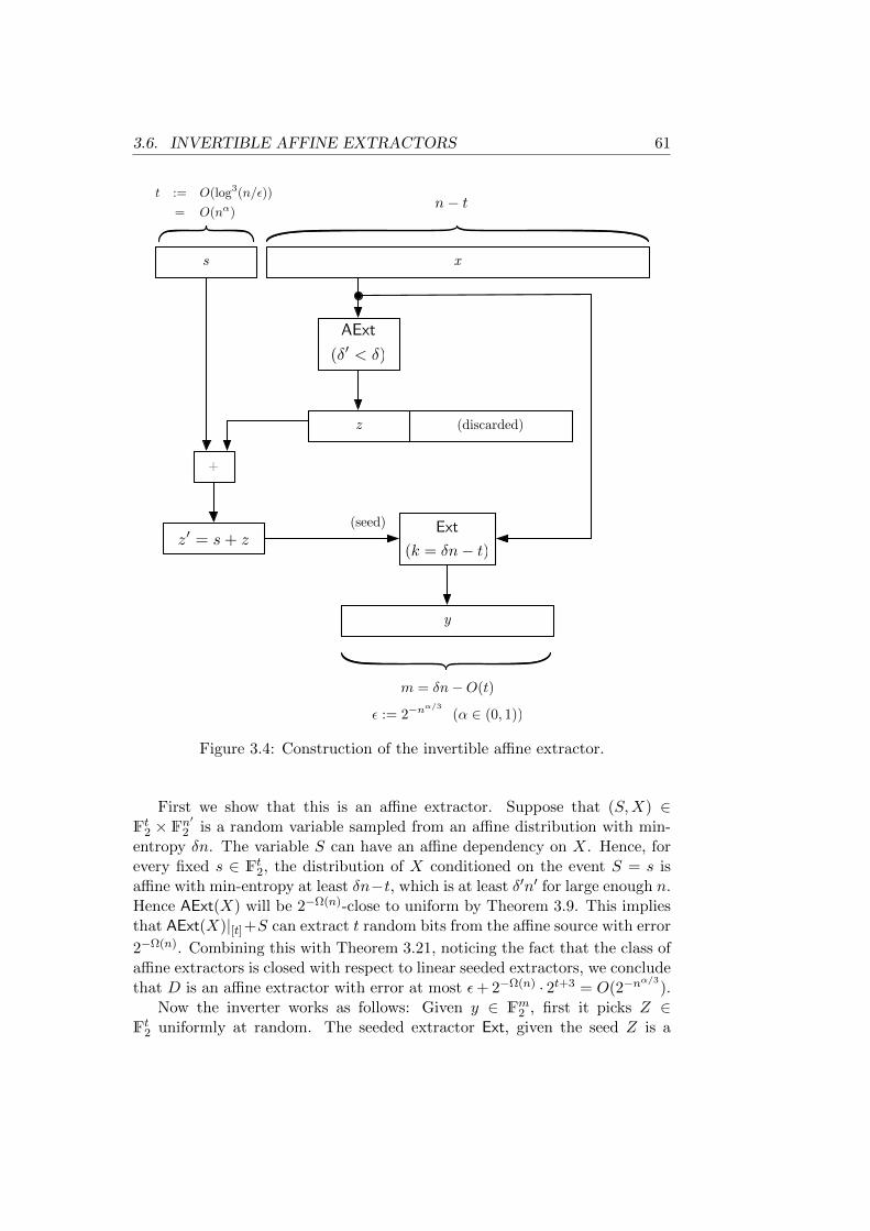
3.6. INVERTIBLE AFFINE EXTRACTORS 61
xs
z (discarded)
+
t := O(log3(n/))
= O(nα)
y
m = δn − O(t)
:= 2−nα/3
(α ∈ (0, 1))
(seed) Ext
(k = δn − t)
AExt
(δ < δ)
z = s + z
n − t
Figure 3.4: Construction of the invertible affine extractor.
First we show that this is an affine extractor. Suppose that (S,X) ∈Ft2 × Fn
′2 is a random variable sampled from an affine distribution with min-
entropy δn. The variable S can have an affine dependency on X. Hence, forevery fixed s ∈ Ft2, the distribution of X conditioned on the event S = s isaffine with min-entropy at least δn−t, which is at least δ′n′ for large enough n.Hence AExt(X) will be 2−Ω(n)-close to uniform by Theorem 3.9. This impliesthat AExt(X)|[t]+S can extract t random bits from the affine source with error
2−Ω(n). Combining this with Theorem 3.21, noticing the fact that the class ofaffine extractors is closed with respect to linear seeded extractors, we concludethat D is an affine extractor with error at most ε+ 2−Ω(n) · 2t+3 = O(2−n
α/3).
Now the inverter works as follows: Given y ∈ Fm2 , first it picks Z ∈Ft2 uniformly at random. The seeded extractor Ext, given the seed Z is a
62 CHAPTER 3. THE WIRETAP CHANNEL PROBLEM
linear function ExtZ : Fn′
2 → Fm2 . Without loss of generality, assume that thisfunction is surjective11. Then the inverter picks X ∈ Fn′2 uniformly at randomfrom the affine subspace defined by the linear constraint ExtZ(X) = y, andoutputs (Z + AExt(X)|[t], X). It is easy to verify that the output is indeeda valid preimage of y. To see the uniformity of the inverter, note that if yis chosen uniformly at random, the distribution of (Z,X) will be uniform onFn2 . Hence (Z + AExt(X)|[t], X), which is the output of the inverter, will beuniform.
In the above construction we are using an affine and a linear seeded extrac-tor as black boxes, and hence, they can be replaced by any other extractors aswell (the construction will achieve an optimal rate provided that the seededextractor extracts almost the entire source entropy). In particular, over largefields one can use the affine and seeded extractors given by Gabizon and Raz[65] that work for sub-constant entropy rates as well.
Moreover, for concreteness we described and instantiated our constructionover the binary field. Observe that Shaltiel’s result, for the special case ofaffine sources, holds regardless of the alphabet size. Moreover, Trevisan’s lin-ear seeded extractor can be naturally extended to handle arbitrary alphabets.Hence, in order to extend our result to non-binary alphabets, it suffices toensure that a suitable seedless affine extractor that supports the desired al-phabet size is available. Bourgain’s original result [16] is stated and provedfor the binary alphabet; however, it seems that this result can be adaptedto work for larger fields as well [17]. Such an extension (along with someimprovements and simplifications) is made explicit by Yehudayoff [167].
An affine extractor is in particular, a symbol-fixing extractor. Hence The-orem 3.24, combined with Lemma 3.15 gives us a wiretap protocol with almostoptimal parameters:
Theorem 3.25. Let δ ∈ [0, 1) and α ∈ (0, 1/3) be constants. Then for aprime power q > 1 and every large enough n there is a (δn,O(2−n
α), 0)q-
resilient wiretap protocol with block length n and rate 1− δ − o(1).
3.7 Further Applications
In this section we will sketch some important applications of our technique tomore general wiretap problems.
11Because the seeded extractor is strong and linear, for most choices of the seed it is agood extractor (by Proposition 2.11), and hence necessarily surjective (if not, one of theoutput symbols would linearly depend on the others and obviously the output distributionwould not be close to uniform). Hence if Ext is not surjective for some seed z, one canreplace it by a trivial surjective linear mapping without affecting its extraction properties.
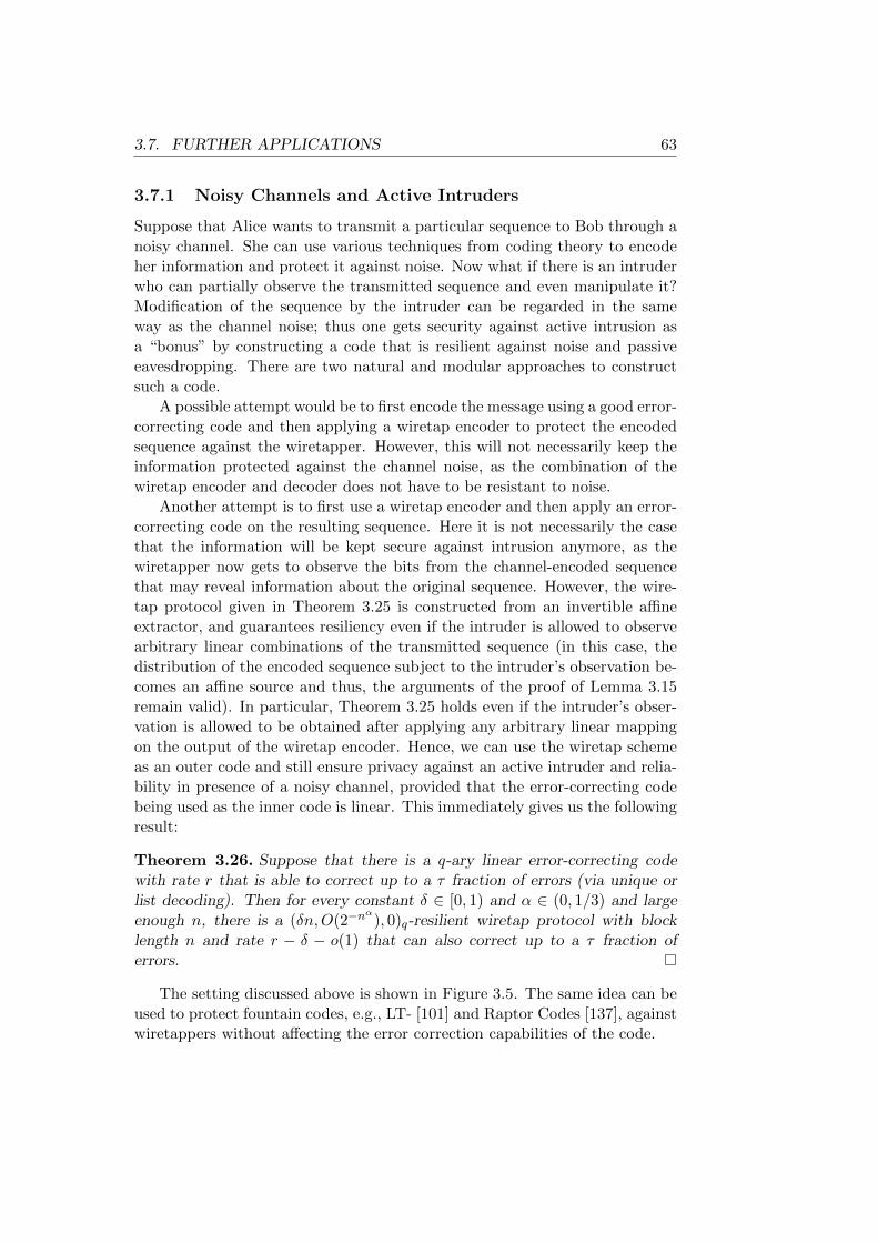
3.7. FURTHER APPLICATIONS 63
3.7.1 Noisy Channels and Active Intruders
Suppose that Alice wants to transmit a particular sequence to Bob through anoisy channel. She can use various techniques from coding theory to encodeher information and protect it against noise. Now what if there is an intruderwho can partially observe the transmitted sequence and even manipulate it?Modification of the sequence by the intruder can be regarded in the sameway as the channel noise; thus one gets security against active intrusion asa “bonus” by constructing a code that is resilient against noise and passiveeavesdropping. There are two natural and modular approaches to constructsuch a code.
A possible attempt would be to first encode the message using a good error-correcting code and then applying a wiretap encoder to protect the encodedsequence against the wiretapper. However, this will not necessarily keep theinformation protected against the channel noise, as the combination of thewiretap encoder and decoder does not have to be resistant to noise.
Another attempt is to first use a wiretap encoder and then apply an error-correcting code on the resulting sequence. Here it is not necessarily the casethat the information will be kept secure against intrusion anymore, as thewiretapper now gets to observe the bits from the channel-encoded sequencethat may reveal information about the original sequence. However, the wire-tap protocol given in Theorem 3.25 is constructed from an invertible affineextractor, and guarantees resiliency even if the intruder is allowed to observearbitrary linear combinations of the transmitted sequence (in this case, thedistribution of the encoded sequence subject to the intruder’s observation be-comes an affine source and thus, the arguments of the proof of Lemma 3.15remain valid). In particular, Theorem 3.25 holds even if the intruder’s obser-vation is allowed to be obtained after applying any arbitrary linear mappingon the output of the wiretap encoder. Hence, we can use the wiretap schemeas an outer code and still ensure privacy against an active intruder and relia-bility in presence of a noisy channel, provided that the error-correcting codebeing used as the inner code is linear. This immediately gives us the followingresult:
Theorem 3.26. Suppose that there is a q-ary linear error-correcting codewith rate r that is able to correct up to a τ fraction of errors (via unique orlist decoding). Then for every constant δ ∈ [0, 1) and α ∈ (0, 1/3) and largeenough n, there is a (δn,O(2−n
α), 0)q-resilient wiretap protocol with block
length n and rate r − δ − o(1) that can also correct up to a τ fraction oferrors.
The setting discussed above is shown in Figure 3.5. The same idea can beused to protect fountain codes, e.g., LT- [101] and Raptor Codes [137], againstwiretappers without affecting the error correction capabilities of the code.
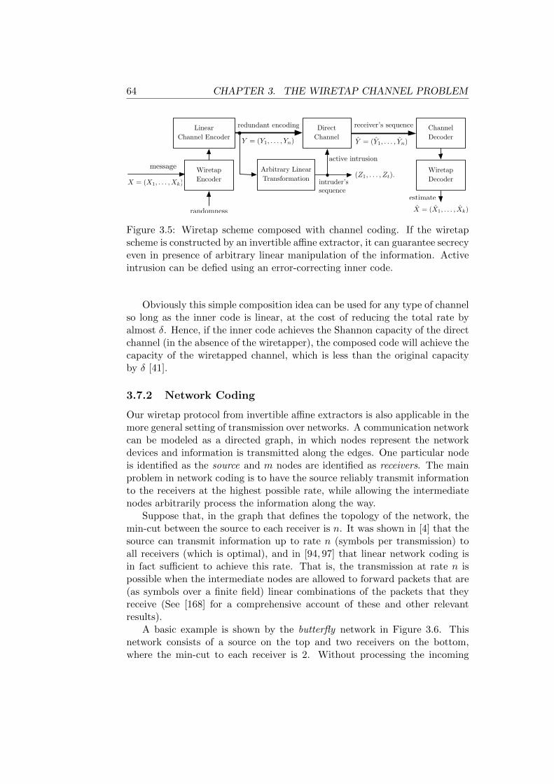
64 CHAPTER 3. THE WIRETAP CHANNEL PROBLEM
LinearChannel Encoder
X = (X1, . . . ,Xk)
Y = (Y1, . . . , Yn)
Direct Channel
message
redundant encoding receiver’s sequence
Y = (Y1, . . . , Yn)
Channel Decoder
estimate
X = (X1, . . . , Xk)randomness
intruder’ssequence
(Z1, . . . , Zt).Arbitrary Linear Transformation
WiretapEncoder
WiretapDecoder
active intrusion
Figure 3.5: Wiretap scheme composed with channel coding. If the wiretapscheme is constructed by an invertible affine extractor, it can guarantee secrecyeven in presence of arbitrary linear manipulation of the information. Activeintrusion can be defied using an error-correcting inner code.
Obviously this simple composition idea can be used for any type of channelso long as the inner code is linear, at the cost of reducing the total rate byalmost δ. Hence, if the inner code achieves the Shannon capacity of the directchannel (in the absence of the wiretapper), the composed code will achieve thecapacity of the wiretapped channel, which is less than the original capacityby δ [41].
3.7.2 Network Coding
Our wiretap protocol from invertible affine extractors is also applicable in themore general setting of transmission over networks. A communication networkcan be modeled as a directed graph, in which nodes represent the networkdevices and information is transmitted along the edges. One particular nodeis identified as the source and m nodes are identified as receivers. The mainproblem in network coding is to have the source reliably transmit informationto the receivers at the highest possible rate, while allowing the intermediatenodes arbitrarily process the information along the way.
Suppose that, in the graph that defines the topology of the network, themin-cut between the source to each receiver is n. It was shown in [4] that thesource can transmit information up to rate n (symbols per transmission) toall receivers (which is optimal), and in [94, 97] that linear network coding isin fact sufficient to achieve this rate. That is, the transmission at rate n ispossible when the intermediate nodes are allowed to forward packets that are(as symbols over a finite field) linear combinations of the packets that theyreceive (See [168] for a comprehensive account of these and other relevantresults).
A basic example is shown by the butterfly network in Figure 3.6. Thisnetwork consists of a source on the top and two receivers on the bottom,where the min-cut to each receiver is 2. Without processing the incoming
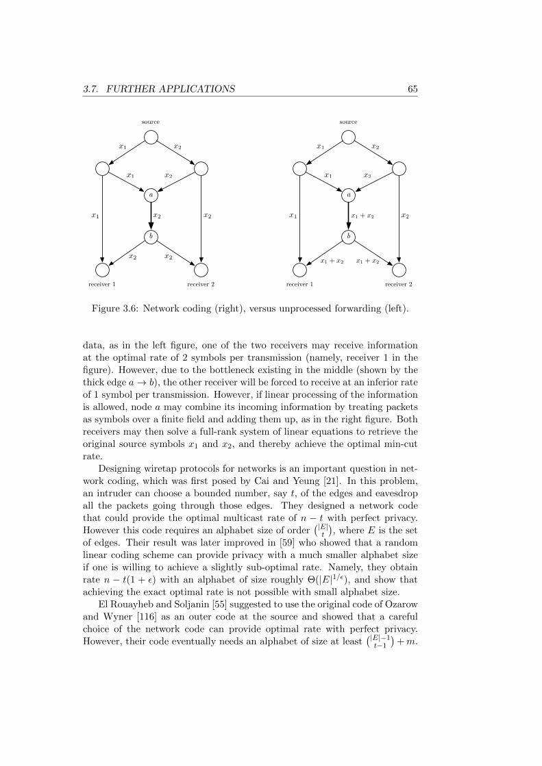
3.7. FURTHER APPLICATIONS 65
a
b
source
receiver 1 receiver 2
x1
x1
x1
x2
x2x2
x2x2
a
b
source
receiver 1 receiver 2
x1
x1
x1
x2
x2x1 + x2
x1 + x2 x1 + x2
x2 x2
Figure 3.6: Network coding (right), versus unprocessed forwarding (left).
data, as in the left figure, one of the two receivers may receive informationat the optimal rate of 2 symbols per transmission (namely, receiver 1 in thefigure). However, due to the bottleneck existing in the middle (shown by thethick edge a→ b), the other receiver will be forced to receive at an inferior rateof 1 symbol per transmission. However, if linear processing of the informationis allowed, node a may combine its incoming information by treating packetsas symbols over a finite field and adding them up, as in the right figure. Bothreceivers may then solve a full-rank system of linear equations to retrieve theoriginal source symbols x1 and x2, and thereby achieve the optimal min-cutrate.
Designing wiretap protocols for networks is an important question in net-work coding, which was first posed by Cai and Yeung [21]. In this problem,an intruder can choose a bounded number, say t, of the edges and eavesdropall the packets going through those edges. They designed a network codethat could provide the optimal multicast rate of n − t with perfect privacy.However this code requires an alphabet size of order
(|E|t
), where E is the set
of edges. Their result was later improved in [59] who showed that a randomlinear coding scheme can provide privacy with a much smaller alphabet sizeif one is willing to achieve a slightly sub-optimal rate. Namely, they obtainrate n − t(1 + ε) with an alphabet of size roughly Θ(|E|1/ε), and show thatachieving the exact optimal rate is not possible with small alphabet size.
El Rouayheb and Soljanin [55] suggested to use the original code of Ozarowand Wyner [116] as an outer code at the source and showed that a carefulchoice of the network code can provide optimal rate with perfect privacy.However, their code eventually needs an alphabet of size at least
(|E|−1t−1
)+m.
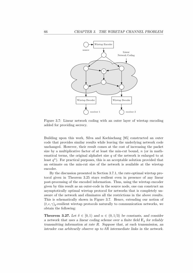
66 CHAPTER 3. THE WIRETAP CHANNEL PROBLEM
+
source
receiver 1
Wiretap Encoder
Wiretap Decoder
receiver 2
Wiretap Decoder
LinearNetwork Coding
Figure 3.7: Linear network coding with an outer layer of wiretap encodingadded for providing secrecy.
Building upon this work, Silva and Kschischang [95] constructed an outercode that provides similar results while leaving the underlying network codeunchanged. However, their result comes at the cost of increasing the packetsize by a multiplicative factor of at least the min-cut bound, n (or in math-ematical terms, the original alphabet size q of the network is enlarged to atleast qn). For practical purposes, this is an acceptable solution provided thatan estimate on the min-cut size of the network is available at the wiretapencoder.
By the discussion presented in Section 3.7.1, the rate-optimal wiretap pro-tocol given in Theorem 3.25 stays resilient even in presence of any linearpost-processing of the encoded information. Thus, using the wiretap encodergiven by this result as an outer-code in the source node, one can construct anasymptotically optimal wiretap protocol for networks that is completely un-aware of the network and eliminates all the restrictions in the above results.This is schematically shown in Figure 3.7. Hence, extending our notion of(t, ε, γ)q-resilient wiretap protocols naturally to communication networks, weobtain the following:
Theorem 3.27. Let δ ∈ [0, 1) and α ∈ (0, 1/3) be constants, and considera network that uses a linear coding scheme over a finite field Fq for reliablytransmitting information at rate R. Suppose that, at each transmission, anintruder can arbitrarily observe up to δR intermediate links in the network.
3.7. FURTHER APPLICATIONS 67
Then the source and the receiver nodes can use an outer code of rate 1−δ−o(1)(obtaining a total rate of R(1− δ)− o(1)) which is completely independent ofthe network, leaves the network code unchanged, and provides almost perfectprivacy with error O(2−R
α) and zero leakage over a q-ary alphabet.
In addition to the above result that uses the invertible affine extractor ofTheorem 3.24, it is possible to use other rate-optimal invertiable affine extrac-tors. In particular, observe that the restricted affine extractor of Theorem 3.11(and in particular, Corollary 3.12) is a linear function (over the extension field)and is thus, obviously has an efficient 0-inverter (since inverting the extractoramounts to solving a system of linear equations). By using this extractor (in-stantiated with Gabidulin’s MRD codes as in Corollary 3.12), we may recoverthe result of Silva and Kschischang [95] in our framework. More precisely, wehave the following result:
Corollary 3.28. Let q be any prime power, and consider a network withminimum cut of size n that uses a linear coding scheme over Fq for reliablytransmitting information at rate R. Suppose that, at each transmission, anintruder can arbitrarily observe up to δR intermediate links in the network,for some δ ∈ [0, 1). Then the source and the receiver nodes can use an outercode of rate 1− δ over Fqn (obtaining a total rate of R(1− δ)) that providesperfect privacy over a qn-ary alphabet.
3.7.3 Arbitrary Processing
In this section we consider the erasure wiretap problem in its most generalsetting, which is still of practical importance. Suppose that the informationemitted by the source goes through an arbitrary communication medium andis arbitrarily processed on the way to provide protection against noise, toobtain better throughput, or for other reasons. Now consider an intruder whois able to eavesdrop a bounded amount of information at various points ofthe channel. One can model this scenario in the same way as the originalpoint-to-point wiretap channel problem, with the difference that instead ofobserving t arbitrarily chosen bits, the intruder now gets to choose an arbitraryBoolean circuit C with t output bits (which captures the accumulation of all theintermediate processing) and observes the output of the circuit when appliedto the transmitted sequence12.
Obviously there is no way to guarantee resiliency in this setting, since theintruder can simply choose C to compute t output bits of the wiretap decoder.However, suppose that in addition there is an auxiliary communication channelbetween the source and the receiver (that we call the side channel) that isseparated from the main channel, and hence, the information passed throughthe two channel do not blend together by the intermediate processing.
12 In fact this models a “harder” problem, as in our problem the circuit C is given by thecommunication scheme and not the intruder. Nevertheless, we consider the harder problem.
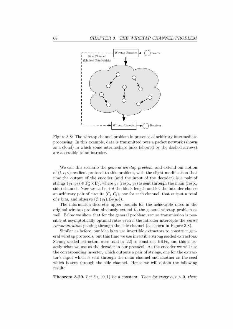
68 CHAPTER 3. THE WIRETAP CHANNEL PROBLEM
Source
Receiver
Side Channel (Limited Bandwidth)
Wiretap Encoder
Wiretap Decoder
Figure 3.8: The wiretap channel problem in presence of arbitrary intermediateprocessing. In this example, data is transmitted over a packet network (shownas a cloud) in which some intermediate links (showed by the dashed arrows)are accessible to an intruder.
We call this scenario the general wiretap problem, and extend our notionof (t, ε, γ)-resilient protocol to this problem, with the slight modification thatnow the output of the encoder (and the input of the decoder) is a pair ofstrings (y1, y2) ∈ Fn2 ×Fd2, where y1 (resp., y2) is sent through the main (resp.,side) channel. Now we call n+ d the block length and let the intruder choosean arbitrary pair of circuits (C1, C2), one for each channel, that output a totalof t bits, and observe (C1(y1), C2(y2)).
The information-theoretic upper bounds for the achievable rates in theoriginal wiretap problem obviously extend to the general wiretap problem aswell. Below we show that for the general problem, secure transmission is pos-sible at asymptotically optimal rates even if the intruder intercepts the entirecommunication passing through the side channel (as shown in Figure 3.8).
Similar as before, our idea is to use invertible extractors to construct gen-eral wiretap protocols, but this time we use invertible strong seeded extractors.Strong seeded extractors were used in [22] to construct ERFs, and this is ex-actly what we use as the decoder in our protocol. As the encoder we will usethe corresponding inverter, which outputs a pair of strings, one for the extrac-tor’s input which is sent through the main channel and another as the seedwhich is sent through the side channel. Hence we will obtain the followingresult:
Theorem 3.29. Let δ ∈ [0, 1) be a constant. Then for every α, ε > 0, there
3.7. FURTHER APPLICATIONS 69
is a (δn, ε, 2−αn + ε)-resilient wiretap protocol for the general wiretap channelproblem that sends n bits through the main channel and d := O(log3(n/ε2))bits through the side channel and achieves rate 1 − δ − α − O(d/(n + d)).The protocol is secure even when the entire communication through the sidechannel is observable by the intruder.
Proof. We will need the following claim in our proof, which is easy to verifyusing an averaging argument:
Claim. Let f : 0, 1n → 0, 1δn be a Boolean function. Then for everyα > 0, and X ∼ Un, the probability that f(X) has fewer than 2n(1−δ−α)
preimages is at most 2−αn.
Now, let Ext be the linear seeded extractor of Theorem 3.22, set up forinput length n, seed length d = O(log3(n/ε2)), min-entropy n(1− δ−α), andoutput length m = n(1−δ−α)−O(d), and error ε2. Then the encoder choosesa seed Z for the extractor uniformly at random and sends it through the sidechannel.
For the chosen value of Z, the extractor is a linear function, and as before,given a message x ∈ 0, 1m, the encoder picks a random vector in the affinesubspace that is mapped by this linear function to x and sends it through thepublic channel.
The decoder, in turn, applies the extractor to the seed received from thesecure channel and the transmitted string. The resiliency of the protocolcan be shown in a similar manner as in Lemma 3.15. Specifically, note thatby the above claim, with probability at least 1− 2−αn, the string transmittedthrough the main channel, conditioned on the observation of the intruder fromthe main channel, has a distribution Y with min-entropy at least n(1− δ−α).Now in addition suppose that the seed z is entirely revealed to the intruder.As the extractor is strong, with probability at least 1− ε, z is a good seed forY, meaning that the output of the extractor applied to Y and seed z is ε-closeto uniform (by Proposition 2.11), and hence the view of the intruder on theoriginal message remains ε-close to uniform.
We observe that it is not possible to guarantee zero leakage for the gen-eral wiretap problem above. Specifically, suppose that (C1, C2) are chosenin a way that they have a single preimage for a particular output (w1, w2).With nonzero probability the observation of the intruder may turn out to be(w1, w2), in which case the entire message is revealed. Nevertheless, it is pos-sible to guarantee negligible leakage as the above theorem does. Moreover,when the general protocol above is used for the original wiretap II problem(where there is no intermediate processing involved), there is no need for aseparate side channel and the entire encoding can be transmitted through asingle channel. Contrary to Theorem 3.25 however, the general protocol willnot guarantee zero leakage even for this special case.
70 CHAPTER 3. THE WIRETAP CHANNEL PROBLEM
3.A Some Technical Details
This appendix is devoted to some technical details that are omitted in themain text of the chapter.
The following proposition quantifies the Shannon entropy of a distributionthat is close to uniform:
Proposition 3.30. Let X be a probability distribution on a finite set S,|S| > 4, that is ε-close to the uniform distribution on S, for some ε ≤ 1/4.Then H(X ) ≥ log2 |S|(1− ε)
Proof. Let n := |S|, and let f(x) := −x log2 x. The function f(x) is concave,passes through the origin and is strictly increasing in the range [0, 1/e]. Fromthe definition, we have H(X ) =
∑s∈S f(PrX (s)). For each term s in this
summation, the probability that X assigns to s is either at least 1/n, whichmakes the corresponding term at least log2 n/n (due to the particular rangeof |S| and ε), or is equal to 1/n − εs, for some εs > 0, in which case theterm corresponding to s is less than log2 n/n by at most εs log2 n (this followsby observing that the slope of the line connecting the origin to the point(1/n, f(1/n)) is log2 n). The bound on the statistical distance implies thatthe differences εs add up to at most ε. Hence, the Shannon entropy of X canbe less than log2 n by at most ε log2 n.
Proposition 3.31. Let (X,Y ) be a pair of random variables jointly dis-tributed on a finite set Ω× Γ. Then13 EY [dist(X|Y,X)] = EX [dist(Y |X,Y )].
Proof. For x ∈ Ω and y ∈ Γ, we will use shorthands px, py, pxy to denotePr[X = x],Pr[Y = y],Pr[X = x, Y = y], respectively. Then we have
EY [dist(X|Y,X)] =∑y∈Γ
pydist(X|(Y = y), X) =1
2
∑y∈Γ
py∑x∈Ω
|pxy/py − px|
=1
2
∑y∈Γ
∑x∈Ω
|pxy − pxpy| =1
2
∑x∈Ω
px∑y∈Γ
|pxy/px − py|
=∑x∈Ω
pxdist(Y |(X = x), Y ) = EX [dist(Y |X,Y )].
Proposition 3.32. Let Ω be a finite set that is partitioned into subsetsS1, . . . , Sk and suppose that X is a distribution on Ω that is γ-close to uni-form. Denote by pi, i = 1, . . . k, the probability assigned to the event Si by
13Here we are abusing the notation and denote by Y the marginal distribution of therandom variable Y , and by Y |(X = a) the distribution of the random variable Y conditionedon the event X = a.
3.A. SOME TECHNICAL DETAILS 71
X . Then ∑i∈[k]
pi · dist(X|Si,USi) ≤ 2γ.
Proof. Let N := |Ω|, and define for each i, γi :=∑
s∈Si
∣∣PrX (s)− 1N
∣∣ , so thatγ1 + · · ·+ γk ≤ 2γ. Observe that by triangle’s inequality, for every i we musthave |pi − |Si|/N | ≤ γi. To conclude the claim, it is enough to show that forevery i, we have dist(X|Si,USi) ≤ γi/pi. This is shown in the following.
pi · dist(X|Si,USi) =pi2
∑s∈Si
∣∣∣∣PrX (s)
pi− 1
|Si|
∣∣∣∣=
1
2
∑s∈Si
∣∣∣∣PrX
(s)− pi|Si|
∣∣∣∣=
1
2
∑s∈Si
∣∣∣∣(PrX
(s)− 1
N
)+
1
|Si|
( |Si|N− pi
)∣∣∣∣≤ 1
2
∑s∈Si
∣∣∣∣PrX
(s)− 1
N
∣∣∣∣+1
2|Si|∑s∈Si
∣∣∣∣ |Si|N − pi∣∣∣∣
≤ γi2
+1
2|Si|· |Si|γi = γi.
The following proposition shows that any function maps close distributionsto close distributions:
Proposition 3.33. Let Ω and Γ be finite sets and f be a function from Ω to Γ.Suppose that X and Y are probability distributions on Ω and Γ, respectively,and let X ′ be a probability distribution on Ω which is δ-close to X . Then iff(X ) ∼ε Y, then f(X ′) ∼ε+δ Y.
Proof. Let X, X ′ and Y be random variables distributed according to X , X ′,and Y, respectively. We want to upperbound∣∣Pr[f(X ′) ∈ T ]− Pr[Y ∈ T ]
∣∣for every T ⊆ Γ. By the triangle inequality, this is no more than∣∣Pr[f(X ′) ∈ T ]− Pr[f(X) ∈ T ]
∣∣+ |Pr[f(X) ∈ T ]− Pr[Y ∈ T ]| .
Here the summand on the right hand side is upperbounded by the distance off(X ) and Y, that is assumed to be at most ε. Let T ′ := x ∈ Ω | f(x) ∈ T.Then the summand on the left can be written as∣∣Pr[X ′ ∈ T ′]− Pr[X ∈ T ′]
∣∣which is at most δ by the assumption that X ∼δ X ′.
72 CHAPTER 3. THE WIRETAP CHANNEL PROBLEM
Omitted Details of the Proof of Corollary 3.19
Here we prove Corollary 3.19 for the case c > 1. The construction is similar tothe case c = 1, and in particular the choice of m and k will remain the same.However, a subtle complication is that the expander family may not have agraph with dm vertices and we need to adapt the extractor of Theorem 3.18to support our parameters, still with exponentially small error. To do so, wepick a graph G in the family with N vertices, such that
cηmdm ≤ N ≤ cηm+1dm,
for a small absolute constant η > 0 that we are free to choose. The assumptionon the expander family guarantees that such a graph exists. Let m′ be thesmallest integer such that dm
′ ≥ cηmN . Index the vertices of G by integers in[N ]. Note that m′ will be larger than m by a constant multiplicative factorthat approaches 1 as η → 0.
For positive integers q and p ≤ q, define the function Modq,p : [q]→ [p] by
Modq,p(x) := 1 + (x mod p).
The extractor SFExt interprets the firstm′ symbols of the input as an integer u,0 ≤ u < dm
′and performs a walk on G starting from the vertex Moddm′ ,N (u+
1), the walk being defined by the remaining input symbols. If the walk reachesa vertex v at the end, the extractor outputs ModN,dm(v)−1, encoded as a d-arystring of length m. A similar argument as in Theorem 3.18 can show that withour choice of the parameters, the extractor has an exponentially small error,where the error exponent is now inferior to that of Theorem 3.18 by O(m),but the constant behind O(·) can be made arbitrarily small by choosing asufficiently small η.
The real difficulty lies with the inverter because Mod is not a balancedfunction (that is, all images do not have the same number of preimages), thuswe will not be able to obtain a perfect inverter. Nevertheless, it is possible toconstruct an inverter with a close-to-uniform output in `∞ norm. This turnsout to be as good as having a perfect inverter, and thanks to the followinglemma, we will still be able to use it to construct a wiretap protocol with zeroleakage:
Lemma 3.34. Suppose that f : [d]n → [d]m is a (k, 2−Ω(m))d symbol-fixingextractor and that X is a distribution on [d]n such that ‖X − U[d]n‖∞ ≤2−Ω(m)/dn. Denote by X ′ the distribution X conditioned on any fixing of atmost n− k coordinates. Then f(X ′) ∼2−Ω(m) U[d]m .
Proof. By Proposition 3.33, it suffices to show that X ′ is 2−Ω(m)-close to an(n, k)d symbol-fixing source. Let S ⊆ [d]m denote the support of X ′, and letε/dn be the `∞ distance between X and U[d]n , so that by our assumption,
ε = 2−Ω(m). By the bound on the `∞ distance, we know that PrX (S) is
3.A. SOME TECHNICAL DETAILS 73
between |S|dn (1 − ε) and |S|
dn (1 + ε). Hence for any x ∈ S, PrX ′(x), which isPrX (x)/PrX (S), is between 1
|S| · 1−ε1+ε and 1
|S| · 1+ε1−ε . This differs from 1/|S| by
at most O(ε)/|S|. Hence, X ′ is 2−Ω(m)-close to US .
In order to invert our new construction, we will need to construct aninverter Invq,p for the function Modq,p. For that, given x ∈ [p] we will justsample uniformly in its preimages. This is where the non-balancedness ofMod causes problems, since if p does not divide q the distribution Invq,p(U[p])is not uniform on [q].
Lemma 3.35. Suppose that q > p. Given a distribution X on [p] such that‖X − U[p]‖∞ ≤ ε
p , we have ‖Invq,p(X )− U[q]‖∞ ≤ 1q ·
p+εqq−p .
Proof. Let X ∼ X and Y ∼ Invq,p(X ). Since we invert the modulo functionby taking for a given output a random preimage uniformly, Pr[Y = y] is equalto Pr[X = Modq,p(y)] divided by the number of y with the same value forModq,p(y). The latter number is either bq/pc or dq/pe, so
1− εpdq/pe ≤ Pr(Y = y) ≤ 1 + ε
pbq/pcBounding the floor and ceiling functions by q/p± 1, we obtain
1− εq + p
≤ Pr(Y = y) ≤ 1 + ε
q − pThat is −p− εq
q(q + p)≤ Pr(Y = y)− 1
q≤ p+ εq
q(q − p) ,
which concludes the proof since this is true for all y.
Now we describe the inverter Inv(x) for the extractor, again abusing thenotation. First the inverter calls InvN,dm(x) to obtain x1 ∈ [N ]. Then itperforms a random walk on the graph, starting from x1, to reach a vertex x2
at the end which is inverted to obtain x3 = Invdm′ ,N (x2) as a d-ary string oflength m′. Finally, the inverter outputs y = (x3, w), where w corresponds theinverse of the random walk of length n−m′. It is obvious that this procedureyields a valid preimage of x.
Using the previous lemma, if x is chosen uniformly, x1 will be at `∞-distance
ε1 :=1
N· dm
N − dm =1
NO(c−ηm).
For a given walk, the distribution of x2 will just be a permutation of thedistribution of x1 and applying the lemma again, we see that the `∞-distanceof x3 from the uniform distribution is
ε2 :=1
dm′· N + ε1d
m′
dm′ −N =1
dm′O(c−ηm).

74 CHAPTER 3. THE WIRETAP CHANNEL PROBLEM
This is true for all the dn−m′
possible walks so the `∞-distance of the distri-bution of y from uniform is bounded by 1
dnO(c−ηm). Applying Lemma 3.34in an argument similar to Lemma 3.15 concludes the proof.
Domenico Scarlatti (1685–1757): Keyboard Sonata
in B minor K. 87 (L. 33).


“War does not determine who isright—only who is left.”
— Bertrand Russell
Chapter 4
Group Testing
The history of group testing is believed to date back to the second WorldWar. During the war, millions of blood samples taken from draftees had tobe subjected to a certain test, and be analyzed in order to identify a fewthousand cases of syphilis. The tests were identical for all the samples. Herethe idea of group testing came to a statistician called Robert Dorfman (andperhaps, a few other researchers working together with him, among themDavid Rosenblatt). He made a very intuitive observation, that, the samplesare constantly subjected to the same test, which is extremely sensitive andremains reliable even if the sample is diluted. Therefore, it makes sense to,instead of analyzing each sample individually, pool every few samples in agroup, and apply the test on the mixture of the samples. If the test outcomeis negative, we will be sure that none of the samples participating in the poolare positive. On the other hand, if the outcome is positive, we know thatone or more of the samples are positive, and will have to proceed with morerefined, or individual, tests in order to identify the individual positives withinthe group.
Since the number of positives in the entire population was suspected to bein order of a few thousands—a small fraction of the population—Dorfman’sidea would save a great deal of time and resources. Whether or not the ideahad been eventually implemented at the time, Dorfman went on to publisha paper on the topic [49], which triggered an extensive line of research incombinatorics known today as combinatorial group testing.
The main challenge in group testing is to design the pools in such a wayto minimize the number of tests required in order to identify the exact set ofpositives. Larger groups would save a lot of tests if their outcome is nega-tive, and are rather wasteful otherwise (since in the latter case they convey arelatively small amount of information).
Of course the applications of group testing are not limited to blood sam-
76
77
pling. To mention another early example, consider a production line of electricitems such as light bulbs (or resistors, capacitors, etc). As a part of the qualityassurance, defective items have to be identified and discarded. Group testingcan be used to aid this process. Suppose that a group of light bulbs are con-nected in series, and an electric current is passed through the circuit. If all thebulbs are illuminated, we can be sure than none is defective, and otherwise,we know that at least one is defective.
Since its emergence decades ago, group testing has found a large numberof surprising applications that are too numerous to be extensively treatedhere. We particularly refer to applications in molecular biology and DNAlibrary screening (cf. [18,58,102,113,130,163,164] and the references therein),multiaccess communication [162], data compression [81], pattern matching[37], streaming algorithms [38], software testing [14], compressed sensing [39],and secure key distribution [26], among others. Moreover, entire books arespecifically targeted to combinatorial group testing [50,51].
In formal terms, the classical group testing problem can be described asfollows. Suppose that we wish to “learn” a Boolean vector of length n, namelyx = (x1, . . . , xn) ∈ 0, 1n using as few questions as possible. Each questioncan ask for a single bit xi, or more generally, specify a group of coordinatesI ⊆ [n] (I 6= ∅) and ask for the bit-wise “or” of the entries at the specifiedcoordinates; i.e.,
∨i∈I xi. We will refer to this type of questions as disjunc-
tive queries. Obviously, in order to be able to uniquely identify x, there is ingeneral no better way than asking for individual bits x1, . . . , xn (and thus, nquestions), since the number of Boolean vectors of length n is 2n and thus,information theoretically, n bits of information is required to describe an ar-bitrary n-bit vector. Therefore, without imposing further restrictions on thepossible realizations of the unknown vector, the problem becomes trivial.
Motivated by the blood sampling application that we just described, natu-ral restriction that is always assumed in group testing on the unknown vectorx is that it is sparse. Namely, for an integer parameter d > 0, we will assumethat the number of nonzero entries of x is at most d. We will refer to such avector as d-sparse. The number of d-sparse Boolean vectors is
n∑i=0
(n
i
)= 2Θ(d log(n/d)),
and therefore, in principle, any d-sparse Boolean vector can be described usingonly O(d log(n/d)) bits of information, a number that can be substantiallysmaller than n if d n. The precise interpretation of the assumption “d n”varies from a setting to another. For a substantial part of this chapter, onecan think of d = O(
√n). The important question in group testing that we
will address in this chapter is that, whether the information-theoretic limitΩ(d log(n/d)) on the number of questions can be achieved using disjunctivequeries as well.
78 CHAPTER 4. GROUP TESTING
Notation for this chapter: In this chapter we will be constantly work-ing with Boolean vectors and their support. The support of a vector x =(x1, . . . , xn) ∈ 0, 1n, denoted by supp(x), is a subset of [n] such that i ∈supp(x) if and only if xi = 1. Thus the Hamming weight of x, that we willdenote by wgt(x) can be defined as wgt(x) = |supp(x)|, and a d-sparse vectorhas the property that wgt(x) ≤ d.
For a matrix M , we denote by M [i, j] the entry of M at the ith row and jthcolumn. Moreover, we denote the ith entry of a vector x by x(i) (assuming aone-to-one correspondence between the coordinate positions of x and naturalnumbers). For an m × n Boolean matrix M and S ⊆ [n], we denote by M |Sthe m × |S| submatrix of M formed by restricting M to the columns pickedby S.
For non-negative integers e0 and e1, we say that an ordered pair of binaryvectors (x, y), each in 0, 1n, are (e0, e1)-close (or x is (e0, e1)-close to y) if ycan be obtained from x by flipping at most e0 bits from 0 to 1 and at moste1 bits from 1 to 0. Hence, such x and y will be (e0 + e1)-close in Hamming-distance. Further, (x, y) are called (e0, e1)-far if they are not (e0, e1)-close.Note that if x and y are seen as characteristic vectors of subsets X and Yof [n], respectively, they are (|Y \X|, |X \ Y |)-close. Furthermore, (x, y) are(e0, e1)-close if and only if (y, x) are (e1, e0)-close.
4.1 Measurement Designs and Disjunct Matrices
Suppose that we wish to correctly identify a d-sparse vector x ∈ 0, 1n usinga reasonable amount of disjunctive queries (that we will simply refer to as“measurements”). In order to do so, consider first the following simple scheme:
1. If n ≤ 2d, trivially measure the vector by querying x1, . . . , xn individu-ally.
2. Otherwise, partition the coordinates of x into b2dc blocks of length eitherbn/(2d)c or dn/(2d)e each, and query the bitwise “or” of the positionswithin each block.
3. At least half of the measurement outcomes must be negative, since thevector x is d-sparse. Recursively run the measurements over the unionof those blocks that have returned positive.
In the above procedure, each recursive call reduces the length of the vec-tor to half or less, which implies that the depth of the recursion is log(n/2d).Moreover, since 2d measurements are made at each level, altogether we willhave O(d log(n/d)) measurements. Therefore, the simple scheme above is op-timal in the sense that it attains the information-theoretic limit Ω(d log(n/d))on the number of measurements, up to constant factors.
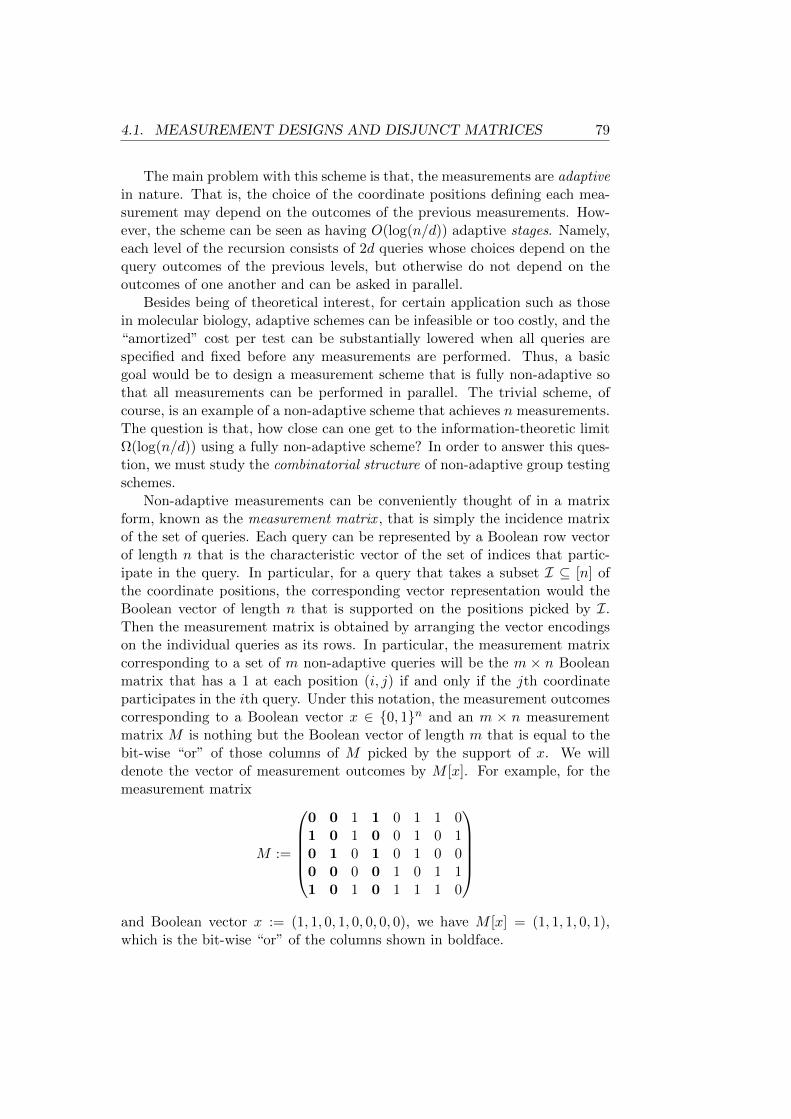
4.1. MEASUREMENT DESIGNS AND DISJUNCT MATRICES 79
The main problem with this scheme is that, the measurements are adaptivein nature. That is, the choice of the coordinate positions defining each mea-surement may depend on the outcomes of the previous measurements. How-ever, the scheme can be seen as having O(log(n/d)) adaptive stages. Namely,each level of the recursion consists of 2d queries whose choices depend on thequery outcomes of the previous levels, but otherwise do not depend on theoutcomes of one another and can be asked in parallel.
Besides being of theoretical interest, for certain application such as thosein molecular biology, adaptive schemes can be infeasible or too costly, and the“amortized” cost per test can be substantially lowered when all queries arespecified and fixed before any measurements are performed. Thus, a basicgoal would be to design a measurement scheme that is fully non-adaptive sothat all measurements can be performed in parallel. The trivial scheme, ofcourse, is an example of a non-adaptive scheme that achieves n measurements.The question is that, how close can one get to the information-theoretic limitΩ(log(n/d)) using a fully non-adaptive scheme? In order to answer this ques-tion, we must study the combinatorial structure of non-adaptive group testingschemes.
Non-adaptive measurements can be conveniently thought of in a matrixform, known as the measurement matrix , that is simply the incidence matrixof the set of queries. Each query can be represented by a Boolean row vectorof length n that is the characteristic vector of the set of indices that partic-ipate in the query. In particular, for a query that takes a subset I ⊆ [n] ofthe coordinate positions, the corresponding vector representation would theBoolean vector of length n that is supported on the positions picked by I.Then the measurement matrix is obtained by arranging the vector encodingson the individual queries as its rows. In particular, the measurement matrixcorresponding to a set of m non-adaptive queries will be the m × n Booleanmatrix that has a 1 at each position (i, j) if and only if the jth coordinateparticipates in the ith query. Under this notation, the measurement outcomescorresponding to a Boolean vector x ∈ 0, 1n and an m × n measurementmatrix M is nothing but the Boolean vector of length m that is equal to thebit-wise “or” of those columns of M picked by the support of x. We willdenote the vector of measurement outcomes by M [x]. For example, for themeasurement matrix
M :=
0 0 1 1 0 1 1 01 0 1 0 0 1 0 10 1 0 1 0 1 0 00 0 0 0 1 0 1 11 0 1 0 1 1 1 0
and Boolean vector x := (1, 1, 0, 1, 0, 0, 0, 0), we have M [x] = (1, 1, 1, 0, 1),which is the bit-wise “or” of the columns shown in boldface.
80 CHAPTER 4. GROUP TESTING
Now suppose that the measurement matrix M is chosen so that it can beused to distinguish between any two d-sparse vectors. In particular, for everyset S ⊆ [n] of indices such that |S| ≤ d − 1, d being the sparsity parameter,the (d− 1)-sparse vector x ∈ 0, 1n supported on S must be distinguishablefrom the d-sparse vector x′ ∈ 0, 1n supported on S ∪ i, for any arbitraryindex i ∈ [n] \ S. Now observe that the Boolean function “or” is monotone.Namely, for a Boolean vector (a1, . . . , an) ∈ 0, 1n that is monotonically lessthan or equal to another vector (b1, . . . , bn) ∈ 0, 1n (i.e., for every j ∈ [n],aj ≤ bj), it must be that ∨
j∈[n]
aj ≤∨j∈[n]
bj .
Therefore, since we have chosen x and x′ so that supp(x) ⊆ supp(x′), we musthave supp(M [x]) ⊆ supp(M [x′]). Since by assumption, M [x] and M [x′] mustdiffer in at least one position, at least one of the rows of M must have anentry 1 at the ith row but all zeros at those corresponding to the set S. Thisis the idea behind the classical notion of disjunct matrices, formally definedbelow (in a slightly generalized form).
Definition 4.1. For integer parameters d, e ≥ 0 (respectively called the spar-sity parameter and noise tolerance), a Boolean matrix is (d, e)-disjunct if forevery choice of d+ 1 distinct columns C0, C1, . . . , Cd of the matrix we have
|supp(C0) \ ∪di=1supp(Ci)| > e.
A (d, 0)-disjunct matrix is simply called d-disjunct.
In the discussion preceding the above definition we saw that the notion of(d− 1)-disjunct matrices is necessary for non-adaptive group testing, in thatany non-adaptive measurement scheme must correspond to a (d− 1)-disjunctmatrix. It turns out that this notion is also sufficient, and thus preciselycaptures the combinatorial structure needed for non-adaptive group testing.
Theorem 4.2. Suppose that M is an m × n matrix that is (d, e)-disjunct.Then for every pair of distinct d-sparse vectors x, x′ ∈ 0, 1n such thatsupp(x) * supp(x′), we have
(4.1) |supp(M [x]) \ supp(M [x′])| > e.
Conversely, if M is such that (4.1) holds for every choice of x, x′ as above,then it must be (d− 1, e)-disjunct.
Proof. For the forward direction, let S := supp(x′) and i ∈ supp(x) \ supp(x′).Then Definition 4.1 implies that there is a set E ⊆ [m] of rows of M suchthat |E| > e and for every j ∈ E, we have M [i, j] = 1 and the jth row ofM restricted to the columns in S (i.e., the support of x′) entirely consists ofzeros. Thus, the measurement outcomes for x′ at positions in E must be zeros
4.1. MEASUREMENT DESIGNS AND DISJUNCT MATRICES 81
while those measurements have a positive outcome for x (since they include atleast one coordinate, namely i, on the support of x). Therefore, (4.1) holds.
For the converse, consider any set S ⊆ [n] of size at most d − 1 andi ∈ [n] \ S. Consider d-sparse vectors x, x′ ∈ 0, 1n such that supp(x′) := Sand supp(x) := S ∪ i. By assumption, there must be a set E ⊆ [m] ofsize larger than e such that, for every j ∈ E, we have M [x](j) = 1 butM [x′](j) = 0. This implies that on those rows of M that are picked by E,the ith entry must be one while those corresponding to S must be zeros.Therefore, M is (d, e)-disjunct.
From the above theorem we know that the measurement outcomes cor-responding to distinct d-sparse vectors differ from one another in more thane positions provided that the measurement matrix is (d, e)-disjunct. Whene > 0, this would allow for distinguishability of sparse vectors even in pres-ence of noise. Namely, even if up to be/2c of the measurements are allowedto be incorrect, it would still possible to uniquely reconstruct the vector be-ing measured. For this reason, we have called the parameter e the “noisetolerance”.
4.1.1 Reconstruction
So far we have focused on combinatorial distinguishability of sparse vectors.However, for applications unique distinguishability is by itself not sufficientand it is important to have efficient “decoding” algorithms to reconstruct thevector being measured.
Fortunately, monotonicity of the “or” function substantially simplifies thedecoding problem. In particular, if two Boolean vectors x, x′ such that thesupport of x is not entirely contained in that of x′ are distinguishable bya measurement matrix, adding new elements to the support of x will nevermake it “less disginguishable” from x′. Moreover, observe that the proof ofTheorem 4.2 never uses sparsity of the vector x. Therefore we see that, (d, e)-disjunct matrices are not only able to distinguish between d-sparse vectors, butmoreover, the only Boolean vector (be it sparse or not) that may reproducethe measurement outcomes resulting from a d-sparse vector x ∈ 0, 1n is xitself. Thus, given a vector of measurement outcomes, in order to reconstructthe sparse vector being measured it suffices to produce any vector that isconsistent with the measurement outcomes. This observation leads us to thefollowing simple decoding algorithm, that we will call the distance decoder :
1. Given a measurement outcome y ∈ 0, 1m, identify the set Sy ⊆ [n] ofthe column indices of the measurement matrix M such that each i ∈ [n]is in Sy if and only if the ith column of M , denoted by ci, satisfies
|supp(ci) \ supp(y)| ≤ be/2c.
82 CHAPTER 4. GROUP TESTING
2. The reconstruction outcome x ∈ 0, 1n is the Boolean vector supportedon Sy.
Lemma 4.3. Let x ∈ 0, 1n be d-sparse and y := M [x], where the mea-surement matrix M is (d, e)-disjunct. Suppose that a measurement outcomey that has Hamming distance at most be/2c with y is given to the distancedecoder. Then the outcome x of the decoder is equal to x.
Proof. Since the distance decoder allows for a “mismatch” of size up to e forthe columns picked by the set Sy, we surely know that supp(x) ⊆ Sy = supp(x).Now suppose that there is an index i ∈ [n] such that i ∈ Sy but i /∈ supp(x).Since M is (d, e)-disjunct, we know that for the ith column ci we have
|supp(ci) \ supp(y)| > e.
On the other hand, since i ∈ Sy, it must be that
|supp(ci) \ supp(y)| ≤ be/2c,
and moreover, by assumption we have that
|supp(y) \ supp(y)| ≤ be/2c.
This is a contradiction. Therefore we must have Sy ⊆ supp(x), implying thatx = x.
4.1.2 Bounds on Disjunct Matrices
So far we have seen that the notion of disjunct matrices is all we need fornon-adaptive group testing. But how small can the number of rows of suchmatrices be? Equivalently, what is the smallest number of measurementsrequired by a non-adaptive group testing scheme that can correctly identifythe support of d-sparse vectors?
4.1.2.1 Upper and Lower Bounds
In the following, we use the probabilistic method to show that, a randomlyconstructed matrix is with overwhelming probability disjunct, and thus obtainan upperbound on the number of the rows of disjunct matrices.
Theorem 4.4. Let p ∈ [0, 1) be an arbitrary real parameter, and d, n beinteger parameters such that d < n. Consider a random m × n Booleanmatrix M such that each entry of M is, independently, chosen to be 1 withprobability q := 1/d. Then there is an m0 = O(d2 log(n/d)/(1 − p)2) ande = Ω(pm/d) such that M is (d, e)-disjunct with probability 1−o(1) providedthat m ≥ m0.
4.1. MEASUREMENT DESIGNS AND DISJUNCT MATRICES 83
Proof. Consider any set S of d columns of M , and any column outside those,say the ith column where i /∈ S. First we upper bound the probability of afailure for this choice of S and i, i.e., the probability that the number of thepositions at the ith column corresponding to which all the columns in S havezeros is at most e. Clearly if this event happens the (d, e)-disjunct property ofM would be violated. On the other hand, if for no choice of S and i a failurehappens the matrix would be indeed (d, e)-disjunct.
Now we compute the failure probability pf for a fixed S and i. A rowis good if at that row the ith column has a 1 but all the columns in S havezeros. For a particular row, the probability that the row is good is q(1− q)d.Then failure corresponds to the event that the number of good rows is atmost e. The distribution of the number of good rows is binomial with meanµ = q(1− q)dm. Choose e := pmq(1− q)d = Ω(pm/d). By a Chernoff bound,the failure probability is at most
pf ≤ exp(−(µ− e)2/(2µ))
≤ exp(−mq(1− p)2/6)
where the second inequality is due to the fact that (1 − q)d = (1 − 1/d)d isalways between 1/3 and 1/2.
Now if we apply a union bound over all possible choices of S and i, theprobability of coming up with a bad choice of M would be at most
n
(n
d
)exp(−mq(1− p)2/6).
This probability vanishes so long asm ≥ m0 for somem0 = O(d2 log(n/d)/(1−p)2).
The above result shows, in particular, that d-disjunct matrices with ncolumns and O(d2 log(n/d)) rows exist. This is by off from the information-theoretic barrier O(d log(n/d)) by a multiplicative factor O(d), which raisesthe question, whether better disjunct matrices can be found. In the literatureof group testing, combinatorial lower bounds on the number of rows of disjunctmatrices exist, which show that the above upper bound is almost the best onecan hope for. In particular, D’yachkov and Rykov [54] have shown that thenumber of rows of any d-disjunct matrices has to be Ω(d2 logd n). Severalother concrete lower bounds on the size of disjunct matrices is known, whichare all asymptotically equivalent (e.g., [63,129]). Moreover, for a nonzero noisetolerance e, the lower bounds can be extended to Ω(d2 logd n+ ed).
4.1.2.2 The Fixed-Input Case
The probabilistic construction of disjunct matrices presented in Theorem 4.4almost surely produces a disjunct matrices using O(d2 log(n/d)) measure-ments. Obviously, due to almost-matching lower bounds, by lowering the
84 CHAPTER 4. GROUP TESTING
number of the measurement the disjunctness property cannot be assured any-more. However, the randomized nature of the designs can be used to ourbenefit to show that, using merely O(d log n) measurements (almost match-ing the information-theoretic lower bound) it is possible (with overwhelmingprobability) to distinguish a “fixed” d-sparse vector from any other (not nec-essarily sparse) vector. More precisely we have the following result, whoseproof is quite similar to that of Theorem 4.4.
Theorem 4.5. Let p ∈ [0, 1) be an arbitrary real parameter, d, n be integerparameters such that d < n, and x ∈ 0, 1n be a fixed d-sparse vector.Consider a random m × n Boolean matrix M such that each entry of Mis, independently, chosen to be 1 with probability q := 1/d. Then there is anm0 = O(d(log n)/(1−p)2) and e = Ω(pm/d) such that, provided that m ≥ m0,with probability 1 − o(1) the following holds: For every y ∈ 0, 1n, y 6= x,the Hamming distance between the outcomes M [y] and M [x] is greater thane.
Proof. We follow essentially the same argument as the proof of Theorem 4.4,but will need a weaker union bound at the end. Call a column i of M good ifthere are more than e rows of M at which the ith column has a 1 but thoseon the support of x (excluding the ith column) have zeros. Now we can followthe argument in the proof of Theorem 4.4 to show that under the conditionsof the theorem, with probability 1−o(1), all columns of M are good (the onlydifference is that, the last union bound will enumerate a set of n possibilitiesrather than (n− 1)
(nd
)).
Now suppose that for the particular outcome of M all columns are good,and take any y ∈ 0, 1n, y 6= x. One of the following cases must be true,and in either case, we show that M [x] and M [y] are different at more than epositions:
1. There is an i ∈ supp(y) \ supp(x): Since the ith column is good, weknow that for more than e rows of M , the entry at the ith column is1 while those at supp(x) are all zeros. This implies that at positionscorresponding to such rows, M [y] must be 1 but M [x] must be zero.
2. We have supp(y) ⊆ supp(x): In this case, take any i ∈ supp(x) \ supp(y),and again use the fact that the ith column is good to conclude that atmore than e positions the outcome M [y] must be zero but M [x] mustbe 1.
As a corollary, the above theorem shows that, with overwhelming proba-bility, once we fix the outcome of the random matrix M constructed by thetheorem, the matrix M will be able to distinguish between most d-sparse vec-tors even in presence of any up to be/2c incorrect measurement outcomes.
4.1. MEASUREMENT DESIGNS AND DISJUNCT MATRICES 85
In particular, we get an average-case result, that there is a fixed measure-ment scheme with only O(d log n) measurements using which it is possible touniquely reconstruct a randomly chosen d-sparse vector (e.g., under the uni-form distribution) with overwhelming probability over the distribution fromwhich the sparse vector is drawn.
4.1.2.3 Sparsity of the Measurements
The probabilistic construction of Theorem 4.4 results in a rather sparse matrix,namely, one with density q = 1/d that decays with the sparsity parameter d.Below we show that sparsity is a necessary condition for the probabilisticconstruction to work at an optimal level on the number of measurements:
Lemma 4.6. Let M be an m × n Boolean random matrix, where m =O(d2 log n) for an integer d > 0, which is constructed by setting each en-try independently to 1 with probability q. Then either q = O(log d/d) orotherwise the probability that M is (d, e)-disjunct (for any e ≥ 0) approachesto zero as n grows.
Proof. Suppose thatM is anm×nmatrix that is (d, e)-disjunct. Observe that,for any integer t ∈ (0, d), if we remove any t columns of M and all the rows onthe support of those columns, the matrix must remain (d− t, e)-disjunct. Thisis because any counterexample for the modified matrix being (d−t, e)-disjunctcan be extended to a counterexample for M being (d, e)-disjunct by addingthe removed columns to its support.
Now consider any t columns of M , and denote by m0 the number of rowsof M at which the entries corresponding to the chosen columns are all zeros.The expected value of m0 is (1− q)tm. Moreover, for any constant δ > 0 wehave
(4.2) Pr[m0 > (1 + δ)(1− q)tm] ≤ exp(−δ2(1− q)tm/4)
by a Chernoff bound.Let t0 be the largest integer for which
(1 + δ)(1− q)t0m ≥ log n.
If t0 < d − 1, we let t := 1 + t0 above, and this makes the right hand sideof (4.2) upper bounded by o(1). So with probability 1 − o(1), the chosen tcolumns of M will keep m0 at most (1 + δ)(1 − q)tm, and removing thosecolumns and m0 rows on their union leaves the matrix (d− t0− 1, e)-disjunct,which obviously requires at least log n rows (as even a (1, 0)-disjunct matrixneeds so many rows). Therefore, we must have
(1 + δ)(1− q)tm ≥ log n
86 CHAPTER 4. GROUP TESTING
or otherwise (with overwhelming probability) M will not be (d, e)-disjunct.But the latter inequality is not satisfied by the assumption on t0. So if t0 <d− 1, little chance remains for M to be (d, e)-disjunct.
Now consider the case t0 ≥ d− 1. Thus, by the choice of t0, we must have
(1 + δ)(1− q)d−1m ≥ log n.
The above inequality implies that we must have
q ≤ log(m(1 + δ)/ log n)
d− 1,
which, for m = O(d2 log n) gives q = O(log d/d).
4.2 Noise resilient schemes and approximatereconstruction
So far, we have introduced the notion of (d, e)-disjunct matrices that can beused in non-adaptive group testing schemes to identify d-sparse vectors up toa number of measurement errors depending on the parameter e. However, asthe existing lower bounds suggest, the number of rows of such matrices cannotreach to the information-theoretic optimum O(d log(n/d)) and moreover, thenoise tolerance e can be at most a factor 1/d of the number of measurements.This motivates two natural questions:
1. Can the number of measurements be lowered at the cost of causinga slight amount of “confusion”? We know, by Theorem 4.5 that, itis possible to identify sparse vectors on average using only O(d log n)measurements. But can something be said in the worst case ?
2. What can be said if the amount of possible errors can be substantiallyhigh; e.g., when a constant fraction of the measurements can producefalse outcomes?
In order to answer the above questions, in this section we introduce a no-tion of measurement schemes that can be “more flexible” than that of disjunctmatrices, and aims to study the trade-off between the amount of errors ex-pected on the measurements versus the ambiguity of the reconstruction. Moreformally we define the following notion.
Definition 4.7. Let m,n, d, e0, e1, e′0, e′1 be integers. An m× n measurement
matrix A is called (e0, e1, e′0, e′1)-resilient for d-sparse vectors if, for every y ∈
0, 1m there exists z ∈ 0, 1n (called a valid decoding of y) such that forevery x ∈ 0, 1n, whenever (x, z) are (e′0, e
′1)-far, (A[x], y) are (e0, e1)-far1.
1 In particular this means that for every x, x′ ∈ 0, 1n, if (A[x], A[x′]) are (e0, e1)-close,then x and x′ must be (e′0 + e′1, e
′0 + e′1)-close.
4.2. NOISE RESILIENT SCHEMES 87
The matrix A is called explicit if it can be computed in polynomial timein its size, and fully explicit if each entry of the matrix can be computed intime poly(m, log n).
Intuitively, the definition states that two measurements are allowed to beconfused only if they are produced from close vectors. The parameters e0
and e′0 correspond to amount of tolerable false positives on the measurementoutcomes and reconstructed vector, where by false positive we mean an errorcaused by mistaking a 0 for 1. Similarly, e1 and e′1 define the amount oftolerable false negatives on both sides, where a false negative occurs when abit that actually must be 1 is flipped to 0.
In particular, an (e0, e1, e′0, e′1)-resilient matrix gives a group testing scheme
that reconstructs the sparse vector up to e′0 false positives and e′1 false neg-atives even in the presence of e0 false positives and e1 false negatives in themeasurement outcome. Under this notation, unique (exact) decoding wouldbe possible using an (e0, e1, 0, 0)-resilient matrix if the amount of measure-ment errors is bounded by at most e0 false positives and e1 false negatives.However, when e′0 + e′1 is positive, decoding may require a bounded amountof ambiguity, namely, up to e′0 false positives and e′1 false negatives in thedecoded sequence.
Observe that the special case of (0, 0, 0, 0)-resilient matrices correspondsto the classical notion of d-disjunct matrices, while a (d, e)-disjunct matrixwould give a (be/2c, be/2c, 0, 0)-resilient matrix for d-sparse vectors.
Definition 4.7 is in fact reminiscent of list-decoding in error-correctingcodes, but with the stronger requirement that the list of decoding possibilitiesmust consist of vectors that are close to one another.
4.2.1 Negative Results
In coding theory, it is possible to construct codes that can tolerate up to aconstant fraction of adversarially chosen errors and still guarantee unique de-coding. Hence it is natural to wonder whether a similar possibility exists ingroup testing, namely, whether there is a measurement matrix that is robustagainst a constant fraction of adversarial errors and still recovers the mea-sured vector exactly. We already have mentioned that this is in general notpossible, since any (d, e)-disjunct matrix (a notion that is necessary for thistask) requires at least de rows, and thus the fraction of tolerable errors bydisjunct matrices cannot be above 1/d. Below we extend this result to themore “asymmetric” notion of resilient matrices, and show that the fraction oftolerable false positives and false negatives must be both below 1/d.
Lemma 4.8. Suppose that an m×n measurement matrix M is (e0, e1, e′0, e′1)-
resilient for d-sparse vectors. Then (maxe0, e1+ 1)/(e′0 + e′1 + 1) ≤ m/d.
88 CHAPTER 4. GROUP TESTING
Proof. We use similar arguments as those used in [20, 75] in the context ofblack-box hardness amplification in NP: Define a partial ordering ≺ betweenbinary vectors using bit-wise comparisons (with 0 < 1). Let t := d/(e′0+e′1+1)be an integer2, and consider any monotonically increasing sequence of vectorsx0 ≺ · · · ≺ xt in 0, 1n where xi has weight i(e′0 + e′1 + 1). Thus, x0 andxt will have weights zero and d, respectively. Note that we must also haveM [x0] ≺ · · · ≺M [xt] due to monotonicity of the “or” function.
A fact that is directly deduced from Definition 4.7 is that, for every x, x′ ∈0, 1n, if (M [x],M [x′]) are (e0, e1)-close, then x and x′ must be (e′0 + e′1, e
′0 +
e′1)-close. This can be seen by setting y := M [x′] in the definition, for whichthere exists a valid decoding z ∈ 0, 1n. As (M [x], y) are (e0, e1)-close, thedefinition implies that (x, z) must be (e′0, e
′1)-close. Moreover, (M [x′], y) are
(0, 0)-close and thus, (e0, e1)-close, which implies that (z, x′) must be (e′1, e′0)-
close. Thus by the triangle inequality, (x, x′) must be (e′0 + e′1, e′0 + e′1)-close.
Now, observe that for all i, (xi, xi+1) are (e′0 + e′1, e′0 + e′1)-far, and hence,
their encodings must be (e0, e1)-far, by the fact we just mentioned. In partic-ular this implies that M [xt] must have weight at least t(e0 +1), which must betrivially upper bounded by m. Hence it follows that (e0 + 1)/(e′0 + e′1 + 1) ≤m/d. Similarly we can also show that (e1 + 1)/(e′0 + e′1 + 1) ≤ m/d.
As shown by the lemma above, tolerance of a measurement matrix againsta constant fraction of errors would make an ambiguity of order Ω(d) in thedecoding inevitable, irrespective of the number of measurements. For mostapplications this might be an unsatisfactory situation, as even a close estimateof the set of positives might not reveal whether any particular individual isdefective or not, and in certain scenarios (such as an epidemic disease or in-dustrial quality assurance) it is unacceptable to miss any defective individuals.This motivates us to focus on approximate reconstructions with one-sided er-ror. Namely, we will require the support of the reconstruction x to alwayscontain the support of the original vector x being measured, and be possiblylarger by up to O(d) positions. It can be argued that, for most applications,such a scheme is as good as exact reconstruction, as it allows one to signif-icantly narrow-down the set of defectives to up to O(d) candidate positives.In particular, as observed in [93], one can use a second stage if necessary andindividually test the resulting set of candidates, using more reliable measure-ments, to identify the exact set of positives. In the literature, such schemesare known as trivial two-stage schemes.
The trade-off given by the following lemma only focuses on false negativesand is thus useful for trivial two-stage schemes:
2For the sake of simplicity in this presentation we ignore the fact that certain fractionsmight in general give non-integer values. However, it should be clear that this will cause noloss of generality.
4.2. NOISE RESILIENT SCHEMES 89
Lemma 4.9. Suppose that an m×n measurement matrix M is (e0, e1, e′0, e′1)-
resilient for d-sparse vectors. Then for every ε > 0, either
e1 <(e′1 + 1)m
εd
or
e′0 ≥(1− ε)(n− d+ 1)
(e′1 + 1)2.
Proof. Let x ∈ 0, 1n be chosen uniformly at random among vectors of weightd. Randomly flip e′1 + 1 of the bits on the support of x to 0, and denote theresulting vector by x′. Using the partial ordering ≺ in the proof of the lastlemma, it is obvious that x′ ≺ x, and hence, M [x′] ≺M [x]. Let b denote anydisjunction of a number of coordinates in x and b′ the same disjunction in x′.We must have
Pr[b′ = 0|b = 1] ≤ e′1 + 1
d,
as for b to be 1 at least one of the variables on the support of x must bepresent in the disjunction and one particular such variable must necessarilybe flipped to bring the value of b′ down to zero. Using this, the expectedHamming distance between M [x] and M [x′] can be bounded as follows:
E[dist(M [x],M [x′])] =∑i∈[m]
1(M [x]i = 1 ∧M [x′]i = 0) ≤ e′1 + 1
d·m,
where the expectation is over the randomness of x and the bit flips, dist(·, ·)denotes the Hamming distance between two vectors, and 1(·) denotes an in-dicator predicate.
Fix a particular choice of x′ that keeps the expectation at most (e′1+1)m/d.Now the randomness is over the possibilities of x, that is, flipping up to e′1 + 1zero coordinates of x′ randomly. Denote by X the set of possibilities of x
for which M [x] and M [x′] are(e′1+1)m
εd -close, and by S the set of all vectorsthat are monotonically larger than x′ and are (e′1 + 1)-close to it. Obviously,X ⊆ S, and, by Markov’s inequality, we know that |X | ≥ (1− ε)|S|.
Let z be any valid decoding of M [x′], Thus, (x′, z) must be (e′0, e′1)-close.
Now assume that e1 ≥ (e′1+1)mεd and consider any x ∈ X . Hence, (M [x],M [x′])
are (e0, e1)-close and (x, z) must be (e′0, e′1)-close by Definition 4.7. Regard
x, x′, z as the characteristic vectors of sets X,X ′, Z ⊆ [n], respectively, whereX ′ ⊆ X. We know that |X \ Z| ≤ e′1 and |X \X ′| = e′1 + 1. Therefore,
(4.3) |(X \X ′) ∩ Z| = |X \X ′| − |X \ Z|+ |X ′ \ Z| > 0,
and z must take at least one nonzero coordinate from supp(x) \ supp(x′).Now we construct an (e′1 + 1)-hypergraph3 H as follows: The vertex set is
[n] \ supp(x′), and for every x ∈ X , we put a hyperedge containing supp(x) \3See Appendix 4.A for definitions.
90 CHAPTER 4. GROUP TESTING
supp(x′). The density of this hypergraph is at least 1 − ε, by the fact that|X | ≥ (1 − ε)S. Now Lemma 4.34 implies that H has a matching of size atleast
t :=(1− ε)(n− d+ 1)
(e′1 + 1)2.
As by (4.3), supp(z) must contain at least one element from the vertices ineach hyperedge of this matching, we conclude that |supp(z) \ supp(x′)| ≥ t,and that e′0 ≥ t.
The lemma above shows that if one is willing to keep the number e′1 of falsenegatives in the reconstruction at the zero level (or bounded by a constant),only an up to O(1/d) fraction of false negatives in the measurements can betolerated (regardless of the number of measurements), unless the number e′0of false positives in the reconstruction grows to an enormous amount (namely,Ω(n) when n− d = Ω(n)) which is certainly undesirable.
Recall that exact reconstruction of d-sparse vectors of length n, even in anoise-free setting, requires at least Ω(d2 logd n) non-adaptive measurements.However, it turns out that there is no such restriction when an approximatereconstruction is sought for, except for the following bound which can beshown using simple counting and holds for adaptive noiseless schemes as well:
Lemma 4.10. Let M be an m× n measurement matrix that is (0, 0, e′0, e′1)-
resilient for d-sparse vectors. Then
m ≥ d log(n/d)− d− e′0 −O(e′1 log((n− d− e′0)/e′1)),
where the last term is defined to be zero for e′1 = 0.
Proof. The proof is a simple counting argument. For integers a > b > 0,we use the notation V (a, b) for the volume of a Hamming ball of radius b in0, 1a. It is given by
V (a, b) =b∑i=0
(a
i
)≤ 2ah(b/a),
where h(·) is the binary entropy function defined as
h(x) := −x log2(x)− (1− x) log2(1− x),
and thus
log V (a, b) ≤ b loga
b+ (a− b) log
a
a− b = Θ(b log(a/b)).
Also, denote by V ′(a, b, e0, e1) the number of vectors in 0, 1a that are (e0, e1)-close to a fixed b-sparse vector. Obviously, V ′(a, b, e0, e1) ≤ V (b, e0)V (a −
4.2. NOISE RESILIENT SCHEMES 91
b, e1). Now consider any (without loss of generality, deterministic) reconstruc-tion algorithm D and let X denote the set of all vectors in 0, 1n that itreturns for some noiseless encoding; that is,
X := x ∈ 0, 1n | ∃y ∈ B, x = D(A[y]),
where B is the set of d-sparse vectors in 0, 1n. Notice that all vectors in Xmust be (d+e′0)-sparse, as they have to be close to the corresponding “correct”decoding. For each vector x ∈ X and y ∈ B, we say that x is matching toy if (y, x) are (e′0, e
′1)-close. A vector x ∈ X can be matching to at most
v := V ′(n, d+ e′0, e′0, e′1) vectors in B, and we upper bound log v as follows:
log v ≤ log V (n−d−e′0, e′1)+log V (d+e′0, e′0) = O(e′1 log((n−d−e′0)/e′1))+d+e′0,
where the term inside O(·) is interpreted as zero when e′1 = 0. Moreover,every y ∈ B must have at least one matching vector in X, namely, D(M [y]).This means that |X| ≥ |B|/v, and that
log |X| ≥ log |B| − log v ≥ d log(n/d)− d− e′0 −O(e′1 log((n− d− e′0)/e′1)).
Finally, we observe that the number of measurements has to be at least |X|to enable D to output all the vectors in X.
According to the lemma, even in the noiseless scenario, any reconstructionmethod that returns an approximation of the sparse vector up to e′0 = O(d)false positives and without false negatives will require Ω(d log(n/d)) measure-ments. As we will show in the next section, an upper bound of O(d log n)is in fact attainable even in a highly noisy setting using only non-adaptivemeasurements. This in particular implies an asymptotically optimal trivialtwo-stage group testing scheme.
4.2.2 A Noise-Resilient Construction
In this section we introduce our general construction and design measurementmatrices for testing d-sparse vectors in 0, 1n. The matrices can be seen asadjacency matrices of certain unbalanced bipartite graphs constructed fromgood randomness condensers or extractors. The main technique that we use toshow the desired properties is the list-decoding view of randomness condensers,extractors, and expanders, developed over the recent years starting from thework of Ta-Shma and Zuckerman on extractor codes [149] and followed byGuruswami, Umans, Vadhan [78] and Vadhan [155].
4.2.2.1 Construction from Condensers
We start by introducing the terms and tools that we will use in our construc-tion and its analysis.
92 CHAPTER 4. GROUP TESTING
Definition 4.11. (mixtures, agreement, and agreement list) Let Σ be a finiteset. A mixture over Σn is an n-tuple S := (S1, . . . , Sn) such that every Si,i ∈ [n], is a nonempty subset of Σ.
The agreement of w := (w1, . . . wn) ∈ Σn with S, denoted by Agr(w, S), isthe quantity
1
n|i ∈ [n] : wi ∈ Si|.
Moreover, we define the quantity
wgt(S) :=∑i∈[n]
|Si|
andρ(S) := wgt(S)/(n|Σ|),
where the latter is the expected agreement of a random vector with S.For example, consider a mixture S := (S1, . . . , S8) over [4]8 where S1 :=
∅, S2 := 1, 3, S3 := 1, 2, S4 := 1, 4, S5 := 1, S6 := 3, S7 := 4, S8 :=1, 2, 3, 4. For this example, we have
Agr((1, 3, 2, 3, 4, 3, 4, 4), S) = 5/8,
and ρ(S) = 13/32.For a code C ⊆ Σn and α ∈ (0, 1], the α-agreement list of C with respect
to S, denoted by LISTC(S, α), is defined as the set4
LISTC(S, α) := c ∈ C : Agr(c, S) > α.
Definition 4.12. (induced code) Let f : Γ × Ω → Σ be a function mappinga finite set Γ × Ω to a finite set Σ. For x ∈ Γ, we use the shorthand f(x) todenote the vector y := (yi)i∈Ω, yi := f(x, i), whose coordinates are indexed bythe elements of Ω in a fixed order. The code induced by f , denoted by C(f) isthe set
f(x) : x ∈ Γ.The induced code has a natural encoding function given by x 7→ f(x).
Definition 4.13. (codeword graph) Let C ⊆ Σn, |Σ| = q, be a q-ary code.The codeword graph of C is a bipartite graph with left vertex set C and rightvertex set n × Σ, such that for every x = (x1, . . . , xn) ∈ C, there is an edgebetween x on the left and (1, x1), . . . , (n, xn) on the right. The adjacencymatrix of the codeword graph is an n|Σ| × |C| binary matrix whose (i, j)thentry is 1 if and only if there is an edge between the ith right vertex and thejth left vertex.
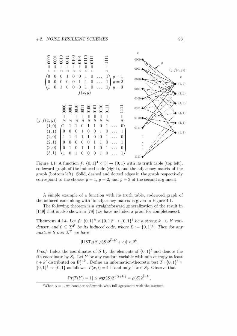
4.2. NOISE RESILIENT SCHEMES 93
(1, 0)
(2, 0)
(3, 0)
(3, 1)
(2, 1)
(1, 1)
. .
. .
.
0000
0001
0010
0011
0100
0101
0110
0111
1111
x
y
(y, f(x, y))x=
0000
x=
0001
x=
0010
x=
0011
x=
0100
x=
0101
x=
0110
x=
0111
x=
111
1
0 0 0 1 0 0 1 0 . . . 10 0 0 0 0 1 1 0 . . . 11 0 1 0 0 0 1 0 . . . 1
y = 1y = 2y = 3
f(x, y)
(y, f(x, y)) x=
0000
x=
0001
x=
0010
x=
0011
x=
0100
x=
010
1
x=
011
0
x=
011
1
x=
111
1(1, 0)(1, 1)(2, 0)(2, 1)(3, 0)(3, 1)
1 1 1 0 1 1 0 1 . . . 00 0 0 1 0 0 1 0 . . . 1
1 1 1 1 1 0 0 1 . . . 00 0 0 0 0 1 1 0 . . . 1
0 1 0 1 1 1 0 1 . . . 01 0 1 0 0 0 1 0 . . . 1
Figure 4.1: A function f : 0, 14× [3]→ 0, 1 with its truth table (top left),codeword graph of the induced code (right), and the adjacency matrix of thegraph (bottom left). Solid, dashed and dotted edges in the graph respectivelycorrespond to the choices y = 1, y = 2, and y = 3 of the second argument.
A simple example of a function with its truth table, codeword graph ofthe induced code along with its adjacency matrix is given in Figure 4.1.
The following theorem is a straightforward generalization of the result in[149] that is also shown in [78] (we have included a proof for completeness):
Theorem 4.14. Let f : 0, 1n × 0, 1t → 0, 1˜be a strong k →ε k
′ con-
denser, and C ⊆ Σ2t be its induced code, where Σ := 0, 1˜. Then for any
mixture S over Σ2t we have
|LISTC(S, ρ(S)2˜−k′ + ε)| < 2k.
Proof. Index the coordinates of S by the elements of 0, 1t and denote theith coordinate by Si. Let Y be any random variable with min-entropy at leastt+ k′ distributed on Ft+k
′
2 . Define an information-theoretic test T : 0, 1˜×0, 1t → 0, 1 as follows: T (x, i) = 1 if and only if x ∈ Si. Observe that
Pr[T (Y ) = 1] ≤ wgt(S)2−(t+k′) = ρ(S)2˜−k′ ,
4When α = 1, we consider codewords with full agreement with the mixture.
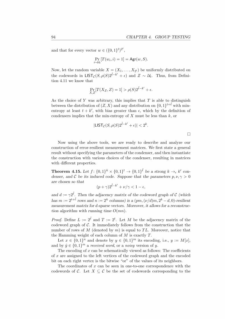
94 CHAPTER 4. GROUP TESTING
and that for every vector w ∈ (0, 1`)2t ,
Pri∼Ut
[T (wi, i) = 1] = Agr(w, S).
Now, let the random variable X = (X1, . . . , X2t) be uniformly distributed on
the codewords in LISTC(S, ρ(S)2˜−k′ + ε) and Z ∼ Ut. Thus, from Defini-
tion 4.11 we know that
PrX,Z
[T (XZ , Z) = 1] > ρ(S)2˜−k′ + ε.
As the choice of Y was arbitrary, this implies that T is able to distinguishbetween the distribution of (Z,X) and any distribution on 0, 1t+˜
with min-entropy at least t + k′, with bias greater than ε, which by the definition ofcondensers implies that the min-entropy of X must be less than k, or
|LISTC(S, ρ(S)2˜−k′ + ε)| < 2k.
Now using the above tools, we are ready to describe and analyze ourconstruction of error-resilient measurement matrices. We first state a generalresult without specifying the parameters of the condenser, and then instantiatethe construction with various choices of the condenser, resulting in matriceswith different properties.
Theorem 4.15. Let f : 0, 1n × 0, 1t → 0, 1˜be a strong k →ε k
′ con-denser, and C be its induced code. Suppose that the parameters p, ν, γ > 0are chosen so that
(p+ γ)2˜−k′ + ν/γ < 1− ε,
and d := γ2˜. Then the adjacency matrix of the codeword graph of C (which
has m := 2t+˜
rows and n := 2n columns) is a (pm, (ν/d)m, 2k − d, 0)-resilientmeasurement matrix for d-sparse vectors. Moreover, it allows for a reconstruc-tion algorithm with running time O(mn).
Proof. Define L := 2˜
and T := 2t. Let M be the adjacency matrix of thecodeword graph of C. It immediately follows from the construction that thenumber of rows of M (denoted by m) is equal to TL. Moreover, notice thatthe Hamming weight of each column of M is exactly T .
Let x ∈ 0, 1n and denote by y ∈ 0, 1m its encoding, i.e., y := M [x],and by y ∈ 0, 1m a received word, or a noisy version of y.
The encoding of x can be schematically viewed as follows: The coefficientsof x are assigned to the left vertices of the codeword graph and the encodedbit on each right vertex is the bitwise “or” of the values of its neighbors.
The coordinates of x can be seen in one-to-one correspondence with thecodewords of C. Let X ⊆ C be the set of codewords corresponding to the

4.2. NOISE RESILIENT SCHEMES 95
support of x. The coordinates of the noisy encoding y are indexed by theelements of [T ]× [L] and thus, y naturally defines a mixture S = (S1, . . . , ST )over [L]T , where Si contains j iff y at position (i, j) is 1.
Observe that ρ(S) is the relative Hamming weight (denoted below by δ(·))of y; thus, we have
ρ(S) = δ(y) ≤ δ(y) + p ≤ d/L+ p = γ + p,
where the last inequality comes from the fact that the relative weight of eachcolumn of M is exactly 1/L and that x is d-sparse.
Furthermore, from the assumption we know that the number of false nega-tives in the measurement is at most νTL/d = νT/γ. Therefore, any codewordin X must have agreement at least 1 − ν/γ with S. This is because S is in-deed constructed from a mixture of the elements in X, modulo false positives(that do not decrease the agreement) and at most νT/γ false negatives eachof which can reduce the agreement by at most 1/T .
Accordingly, we consider a decoder which, similar to the distance decoderthat we have introduced before, simply outputs a binary vector x supportedon the coordinates corresponding to those codewords of C that have agreementlarger than 1− ν/γ with S. Clearly, the running time of the decoder is linearin the size of the measurement matrix.
By the discussion above, x must include the support of x. Moreover,Theorem 4.14 applies for our choice of parameters, implying that x must haveweight less than 2k.
4.2.2.2 Instantiations
Now we instantiate the general result given by Theorem 4.15 with variouschoices of the underlying condenser, among the results discussed in Section 2.3,and compare the obtained parameters. First, we consider two extreme cases,namely, a non-explicit optimal condenser with zero overhead (i.e., extractor)and then a non-explicit optimal condenser with zero loss (i.e., lossless con-denser) and then consider how known explicit constructions can approach theobtained bounds. A summary of the obtained results is given in Table 4.1.
Optimal Extractors
Recall Radhakrishan and Ta-Shma’s non-constructive bound that for everychoice of the parameters k, n, ε, there is a strong (k, ε)-extractor with inputlength n, seed length t = log(n − k) + 2 log(1/ε) + O(1) and output length˜= k−2 log(1/ε)−O(1), and that the bound is achieved by a random function.Plugging this result in Theorem 4.15, we obtain a non-explicit measurementmatrix from a simple, randomized construction that achieves the desired trade-off with high probability:
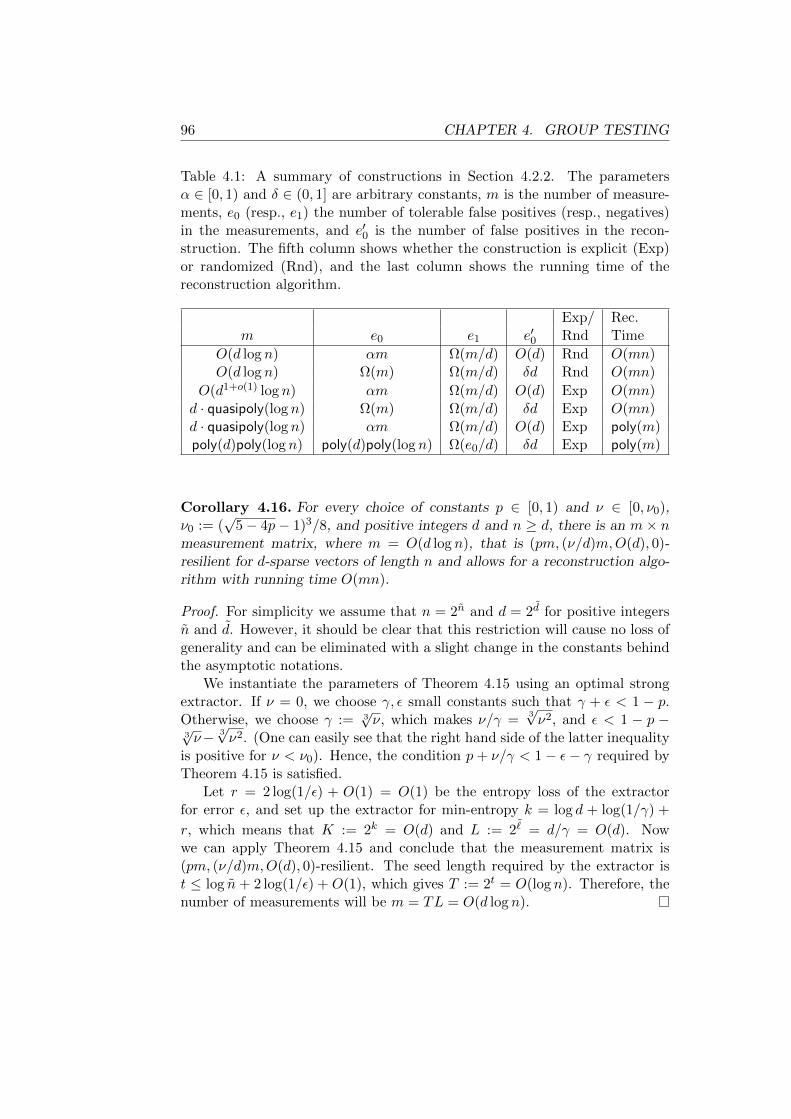
96 CHAPTER 4. GROUP TESTING
Table 4.1: A summary of constructions in Section 4.2.2. The parametersα ∈ [0, 1) and δ ∈ (0, 1] are arbitrary constants, m is the number of measure-ments, e0 (resp., e1) the number of tolerable false positives (resp., negatives)in the measurements, and e′0 is the number of false positives in the recon-struction. The fifth column shows whether the construction is explicit (Exp)or randomized (Rnd), and the last column shows the running time of thereconstruction algorithm.
Exp/ Rec.m e0 e1 e′0 Rnd Time
O(d log n) αm Ω(m/d) O(d) Rnd O(mn)O(d log n) Ω(m) Ω(m/d) δd Rnd O(mn)
O(d1+o(1) log n) αm Ω(m/d) O(d) Exp O(mn)d · quasipoly(log n) Ω(m) Ω(m/d) δd Exp O(mn)d · quasipoly(log n) αm Ω(m/d) O(d) Exp poly(m)poly(d)poly(log n) poly(d)poly(log n) Ω(e0/d) δd Exp poly(m)
Corollary 4.16. For every choice of constants p ∈ [0, 1) and ν ∈ [0, ν0),ν0 := (
√5− 4p− 1)3/8, and positive integers d and n ≥ d, there is an m× n
measurement matrix, where m = O(d log n), that is (pm, (ν/d)m,O(d), 0)-resilient for d-sparse vectors of length n and allows for a reconstruction algo-rithm with running time O(mn).
Proof. For simplicity we assume that n = 2n and d = 2d for positive integersn and d. However, it should be clear that this restriction will cause no loss ofgenerality and can be eliminated with a slight change in the constants behindthe asymptotic notations.
We instantiate the parameters of Theorem 4.15 using an optimal strongextractor. If ν = 0, we choose γ, ε small constants such that γ + ε < 1 − p.Otherwise, we choose γ := 3
√ν, which makes ν/γ =
3√ν2, and ε < 1 − p −
3√ν− 3√ν2. (One can easily see that the right hand side of the latter inequality
is positive for ν < ν0). Hence, the condition p+ ν/γ < 1− ε− γ required byTheorem 4.15 is satisfied.
Let r = 2 log(1/ε) + O(1) = O(1) be the entropy loss of the extractorfor error ε, and set up the extractor for min-entropy k = log d + log(1/γ) +
r, which means that K := 2k = O(d) and L := 2˜
= d/γ = O(d). Nowwe can apply Theorem 4.15 and conclude that the measurement matrix is(pm, (ν/d)m,O(d), 0)-resilient. The seed length required by the extractor ist ≤ log n + 2 log(1/ε) + O(1), which gives T := 2t = O(log n). Therefore, thenumber of measurements will be m = TL = O(d log n).
4.2. NOISE RESILIENT SCHEMES 97
Optimal Lossless Condensers
Now we instantiate Theorem 4.15 with an optimal strong lossless condenserwith input length n, entropy requirement k, seed length t = log n+ log(1/ε) +O(1) and output length ˜ = k + log(1/ε) + O(1). Thus we get the followingcorollary.
Corollary 4.17. For positive integers n ≥ d and every constant δ > 0 there isan m×n measurement matrix, where m = O(d log n), that is (Ω(m),Ω(1/d)m,δd, 0)-resilient for d-sparse vectors of length n and allows for a reconstructionalgorithm with running time O(mn).
Proof. We will use the notation of Theorem 4.15 and apply it using an optimalstrong lossless condenser. This time, we set up the condenser with errorε := 1
2δ/(1 + δ) and min-entropy k such that K := 2k = d/(1 − 2ε). As the
error is a constant, the overhead and hence 2˜−k will also be a constant. The
seed length is t = log(n/ε) + O(1), which makes T := 2t = O(log n). As
L := 2˜
= O(d), the number of measurements becomes m = TL = O(d log n),as desired.
Moreover, note that our choice of K implies that K − d = δd. Thus weonly need to choose p and ν appropriately to satisfy the condition
(4.4) (p+ γ)L/K + ν/γ < 1− ε,
where γ = d/L = K/(L(1 + δ)) is a constant, as required by the lemma.Substituting for γ in (4.4) and after simple manipulations, we get the condition
pL/K + ν(L/K)(1 + δ) <δ
2(1 + δ),
which can be satisfied by choosing p and ν to be appropriate positive constants.
Both results obtained in Corollaries 4.16 and 4.17 almost match the lowerbound of Lemma 4.10 for the number of measurements. However, we note thefollowing distinction between the two results: Instantiating the general con-struction of Theorem 4.15 with an extractor gives us a sharp control over thefraction of tolerable errors, and in particular, we can obtain a measurementmatrix that is robust against any constant fraction (bounded from 1) of falsepositives. However, the number of potential false positives in the reconstruc-tion will be bounded by some constant fraction of the sparsity of the vectorthat cannot be made arbitrarily close to zero.
On the other hand, using a lossless condenser enables us to bring down thenumber of false positives in the reconstruction to an arbitrarily small fractionof d (which is, in light of Lemma 4.8, the best we can hope for), though it doesnot give as good a control on the fraction of tolerable errors as in the extractorcase, though we still obtain resilience against the same order of errors.
98 CHAPTER 4. GROUP TESTING
Recall that the simple divide-and-conquer adaptive construction givenin beginning the chapter consists of O(log(n/d)) non-adaptive stages, wherewithin each stage O(d) non-adaptive measurements are made, but the choiceof the measurements for each stage fully depends on all the previous out-comes. By the lower bounds on the size of disjunct matrices, we know thatthe number of non-adaptive rounds cannot be reduced to 1 without affectingthe total number of measurements by a multiplicative factor of Ω(d). How-ever, our non-adaptive upper bounds (Corollaries 4.16 and 4.17) show thatthe number of rounds can be reduced to 2, while preserving the total numberof measurements at O(d log n). In particular, in a two-stage scheme, the firstnon-adaptive round would output an approximation of the d-sparse vector upto O(d) false positive (even if the measurements are highly unreliable) andthe second round simply examines the O(d) possible positions using trivialsingleton measurements to pinpoint the exact support of the vector.
Applying the Guruswami-Umans-Vadhan’s Extractor
While Corollaries 4.16 and 4.17 give probabilistic constructions of noise-resi-lient measurement matrices, certain applications require a fully explicit ma-trix that is guaranteed to work. To that end, we need to instantiate Theo-rem 4.15 with an explicit condenser. First, we use the nearly-optimal explicitextractor of Guruswami, Umans and Vadhan (Theorem 2.24), that currentlygives the best trade-off for the range of parameters needed for our applica-tion. Using this extractor, we obtain a similar trade-off as in Corollary 4.16,except for a higher number of measurements which would be bounded byO(2O(log2 log d)d log n) = O(d1+o(1) log n).
Corollary 4.18. For every choice of constants p ∈ [0, 1) and ν ∈ [0, ν0),ν0 := (
√5− 4p − 1)3/8, and positive integers d and n ≥ d, there is a fully
explicit m× n measurement matrix, where
m = O(2O(log2 log d)d log n) = O(d1+o(1) log n),
that is (pm, (ν/d)m,O(d), 0)-resilient for d-sparse vectors of length n and al-lows for a reconstruction algorithm with running time O(mn).
Applying “Zig-Zag” Lossless Condenser
An important explicit construction of lossless condensers that has an almostoptimal output length is due to Capalbo et al. [23]. This construction borrowsthe notion of “zig-zag products” that is a combinatorial tool for constructionof expander graphs as a major ingredient of the condenser. The followingtheorem quotes a setting of this construction that is most useful for our ap-plication:
4.2. NOISE RESILIENT SCHEMES 99
Theorem 4.19. [23] For every k ≤ n ∈ N, ε > 0 there is an explicit k →ε kcondenser5 with seed length d = O(log3(n/ε)) and output length m = k +log(1/ε) +O(1).
Combining Theorem 4.15 with the above condenser, we obtain a similarresult as in Corollary 4.17, except that the number of measurements would bed2log3(logn) = d · quasipoly(log n).
Corollary 4.20. For positive integers n ≥ d and every constant δ > 0 thereis a fully explicit m× n measurement matrix, where
m = d2log3(logn) = d · quasipoly(log n),
that is (Ω(m),Ω(1/d)m, δd, 0)-resilient for d-sparse vectors of length n andallows for a reconstruction algorithm with running time O(mn).
4.2.2.3 Measurements Allowing Sublinear Time Reconstruction
The naive reconstruction algorithm given by Theorem 4.15 works efficientlyin linear time in the size of the measurement matrix. However, for very sparsevectors (i.e., d n), it might be of practical importance to have a recon-struction algorithm that runs in sublinear time in n, the length of the vec-tor, and ideally, polynomial in the number of measurements, which is merelypoly(log n, d) if the number of measurements is optimal.
As shown in [149], if the code C in Theorem 4.14 is obtained from a strongextractor constructed from a black-box pseudorandom generator (PRG), it ispossible to compute the agreement list (which is guaranteed by the theoremto be small) more efficiently than a simple exhaustive search over all possiblecodewords. In particular, in this case they show that LISTC(S, ρ(S)+ε) can be
computed in time poly(2t, 2˜, 2k, 1/ε) (where t, ˜, k, ε are respectively the seed
length, output length, entropy requirement, and error of the extractor), whichcan be much smaller than 2n (n being the input length of the extractor).
Currently two constructions of extractors from black-box PRGs are known:Trevisan’s extractor [152] (as well as its improvement in [123]) and Shaltiel-Umans’ extractor [134]. However, the latter can only extract a sub-constantfraction of the min-entropy and is not suitable for our needs, albeit it requiresa considerably shorter seed than Trevisan’s extractor. Thus, here we onlyconsider Raz’s improvement of Trevisan’s extractor given in Theorem 2.20.Using this extractor in Theorem 4.15, we obtain a measurement matrix forwhich the reconstruction is possible in polynomial time in the number ofmeasurements; however, as the seed length required by this extractor is largerthan Theorem 2.24, we will now require a higher number of measurementsthan before. Specifically, using Trevisan’s extractor, we get the following.
5Though not explicitly mentioned in [23], these condensers can be considered to bestrong.
100 CHAPTER 4. GROUP TESTING
Corollary 4.21. For every choice of constants p ∈ [0, 1) and ν ∈ [0, ν0),ν0 := (
√5− 4p − 1)3/8, and positive integers d and n ≥ d, there is a fully
explicit m× n measurement matrix M that is (pm, (ν/d)m,O(d), 0)-resilientfor d-sparse vectors of length n, where
m = O(d2log3 logn) = d · quasipoly(log n).
Furthermore, M allows for a reconstruction algorithm with running timepoly(m), which would be sublinear in n for d = O(nc) and a suitably smallconstant c > 0.
On the condenser side, we observe that the strong lossless (and lossy)condensers due to Guruswami et al. (given in Theorem 2.22) also allow ef-ficient list-recovery. The code induced by this condenser is precisely a list-decodable code due to Parvaresh and Vardy [118]. Thus, the efficient listrecovery algorithm of the condenser is merely the list-decoding algorithm forthis code6. Combined with Theorem 4.15, we can show that codeword graphsof Parvaresh-Vardy codes correspond to good measurement matrices that al-low sublinear time recovery, but with incomparable parameters to what weobtained from Trevisan’s extractor (the proof is similar to Corollary 4.17):
Corollary 4.22. For positive integers n ≥ d and any constants δ, α > 0 thereis an m× n measurement matrix, where
m = O(d3+α+2/α(log n)2+2/α),
that is (Ω(e),Ω(e/d), δd, 0)-resilient for d-sparse vectors of length n, where
e := (log n)1+1/αd2+1/α.
Moreover, the matrix allows for a reconstruction algorithm with running timepoly(m).
We remark that we could also use a lossless condenser due to Ta-Shma etal. [148] which is based on Trevisan’s extractor and also allows efficient listrecovery, but it achieves inferior parameters compared to Corollary 4.22.
4.2.2.4 Connection with List-Recoverability
Extractor codes that we used in Theorem 4.15 are instances of soft-decisiondecodable codes7 that provide high list-decodability in “extremely noisy” sce-narios. In fact it is not hard to see that good extractors or condensers are
6 For similar reasons, any construction of measurement matrices based on codewordgraphs of algebraic codes that are equipped efficient soft-decision decoding (including theoriginal Reed-Solomon based construction of Kautz and Singleton [89]) allow sublinear timereconstruction.
7To be precise, here we are dealing with a special case of soft-decision decoding withbinary weights.
4.2. NOISE RESILIENT SCHEMES 101
required for our construction to carry through, as Theorem 4.14 can be shownto hold, up to some loss in parameters, in the reverse direction as well (asalready shown by Ta-Shma and Zuckerman [149, Theorem 1] for the case ofextractors).
However, for designing measurement matrices for the noiseless (or low-noise) case, it is possible to resort to the slightly weaker notion of list recover-able codes. Formally, a code C of block length n over an alphabet Σ is called(α, d, ˜)-list recoverable if for every mixture S over Σn consisting of sets ofsize at most d each, we have |LISTC(S, α)| ≤ ˜. A simple argument similarto Theorem 4.15 shows that the adjacency matrix of the codeword graph ofsuch a code with rate R gives a (log n)|Σ|/R × n measurement matrix8 ford-sparse vectors in the noiseless case with at most ˜− d false positives in thereconstruction.
Ideally, a list-recoverable code with α = 1, alphabet size O(d), positiveconstant rate, and list size ˜ = O(d) would give an O(d log n) × n matrix ford-sparse vectors, which is almost optimal (furthermore, the recovery wouldbe possible in sublinear time if C is equipped with efficient list recovery).However, no explicit construction of such a code is so far known.
Two natural choices of codes with good list-recoverability properties areReed-Solomon and Algebraic-Geometric codes, which in fact provide soft-decision decoding with short list size (cf. [74]). However, while the list size ispolynomially bounded by n and d, it can be much larger than O(d) that weneed for our application even if the rate is polynomially small in d.
On the other hand, it is shown in [77] that folded Reed-Solomon Codes arelist-recoverable with constant rate, but again they suffer from large alphabetand list size9.
We also point out a construction of (α, d, d) list-recoverable codes (allowinglist recovery in time O(nd)) in [77] with rate polynomially small but alphabetsize exponentially large in d, from which they obtain superimposed codes.
4.2.2.5 Connection with the Bit-Probe Model and Designs
An important problem in data structures is the static set membership problemin bit-probe model, which is the following: Given a set S of at most d elementsfrom a universe of size n, store the set as a string of length m such that anyquery of the type “is x in S?” can be reliably answered by reading few bits ofthe encoding. The query algorithm might be probabilistic, and be allowed toerr with a small one or two-sided error. Information theoretically, it is easy to
8For codes over large alphabets, the factor |Σ| in the number of rows can be improvedusing concatenation with a suitable inner measurement matrix.
9As shown in [78], folded Reed-Solomon codes can be used to construct lossless con-densers, which eliminates the list size problem. However, they give inferior parameterscompared to Parvaresh-Vardy codes used in Corollary 4.22.
102 CHAPTER 4. GROUP TESTING
see that m = Ω(d log(n/d)) regardless of the bit-probe complexity and even ifa small constant error is allowed.
Remarkably, it was shown in [19] that the lower bound on m can be (non-explicitly) achieved using only one bit-probe. Moreover, a part of their workshows that any one-probe scheme with negative one-sided error ε (where thescheme only errs in case x /∈ S) gives a bd/εc-superimposed code (and hence,requires m = Ω(d2 log n) by [54]). It follows that from any such scheme one canobtain a measurement matrix for exact reconstruction of sparse vectors, which,by Lemma 4.8, cannot provide high resiliency against noise. The conversedirection, i.e., using superimposed codes to design bit-probe schemes does notnecessarily hold unless the error is allowed to be very close to 1. However,in [19] combinatorial designs10 based on low-degree polynomials are used toconstruct one bit-probe schemes with m = O(d2 log2 n) and small one-sidederror.
On the other hand, Kautz and Singleton [89] observed that the encoding ofa combinatorial design as a binary matrix corresponds to a superimposed code(which is in fact slightly error-resilient). Moreover, they used Reed-Solomoncodes to construct a design, which in particular gives a d-superimposed code.This is in fact the same design that is used in [19], and in our terminology, canbe regarded as the adjacency matrix of the codeword graph of a Reed-Solomoncode.
It is interesting to observe the intimate similarity between our frameworkgiven by Theorem 4.15 and classical constructions of superimposed codes.However, some key differences are worth mentioning. Indeed, both construc-tions are based on codeword graphs of error-correcting codes. However, classi-cal superimposed codes owe their properties to the large distance of the under-lying code. On the other hand, our construction uses extractor and condensercodes and does not give a superimposed code simply because of the substan-tially low number of measurements. However, as shown in Theorem 4.15, theyare good enough for a slight relaxation of the notion of superimposed codesbecause of their soft-decision list decodability properties, which additionallyenables us to attain high noise resilience and a considerably smaller numberof measurements.
Interestingly, Buhrman et al. [19] use randomly chosen bipartite graphs toconstruct storage schemes with two-sided error requiring nearly optimal spaceO(d log n), and Ta-Shma [147] later shows that expander graphs from losslesscondensers would be sufficient for this purpose. However, unlike schemeswith negative one-sided error, these schemes use encoders that cannot beimplemented by the “or” function and thus do not translate to group testingschemes.
10 A design is a collection of subsets of a universe, each of the same size, such that thepairwise intersection of any two subset is upper bounded by a prespecified parameter.
4.3. THE THRESHOLD MODEL 103
4.3 The Threshold Model
A natural generalization of classical group testing, introduced by Damaschke[42], considers the case where the measurement outcomes are determined bya threshold predicate instead of logical “or”.
In particular, the threshold model is characterized by two integer param-eters `, u such that 0 < ` ≤ u (that are considered to be fixed constants), andeach measurement outputs positive if the number of positives within the cor-responding pool is at least u. On the other hand, if the number of positivesis less than `, the test returns negative, and otherwise the outcome can bearbitrary. In this view, classical group testing corresponds to the special casewhere ` = u = 1. In addition to being of theoretical interest, the thresholdmodel is interesting for applications, in particular in biology, where the mea-surements have reduced or unpredictable sensitivity or may depend on variousfactors that must be simultaneously present in the sample.
The difference g := u − ` between the thresholds is known as the gapparameter. As shown by Damaschke [42], in threshold group testing identifi-cation of the set of positives is only possible when the number of positives is atleast u. Moreover, regardless of the number of measurements, in general theset of positives can only be identified within up to g false positives and g falsenegatives (thus, unique identification can be guaranteed only when ` = u).
Additionally, Damaschke constructed a scheme for identification of thepositives in the threshold model. For the gap-free case where g = 0, thenumber of measurements in this scheme is O((d + u2) log n), which is nearlyoptimal (within constant factors). However, when g > 0, the number ofmeasurements becomes O(dnb + du), for an arbitrary constant b > 0, if upto g + (u − 1)/b misclassifications are allowed. Moreover, Chang et al. [24]have proposed a different scheme for the gap-free case that achieves O(d log n)measurements.
A drawback of the scheme presented by Damaschke (as well as the oneby Chang et al.) is that the measurements are adaptive. As mentioned be-fore, for numerous applications (in particular, molecular biology), adaptivemeasurements are infeasible and must be avoided.
In this section, we consider the non-adaptive threshold testing problemin a possibly noisy setting, and develop measurement matrices that can beused in the threshold model. Similar to the classical model of group testing,non-adaptive measurements in the threshold model can be represented as aBoolean matrix, where the ith row is the characteristic vector of the set ofitems that participate in the ith measurement.
4.3.1 Strongly Disjunct Matrices
Non-adaptive threshold testing has been considered by Chen and Fu [27].They observe that, a generalization of the standard notion of disjunct matrices
104 CHAPTER 4. GROUP TESTING
(the latter being extensively used in the literature of classical group testing)is suitable for the threshold model. In this section, we refer to this generalizednotion as strongly disjunct matrices and to the standard notion as classicaldisjunct matrices. Strongly disjunct matrices can be defined as follows.
Definition 4.23. A Boolean matrix (with at least d + u columns) is said tobe strongly (d, e;u)-disjunct if for every choice of d+ u distinct columns
C1, . . . , Cu, C′1, . . . , C
′d,
all distinct, we have
| ∩ui=1 supp(Ci) \ ∪di=1supp(C ′i)| > e.
Observe that, (d, e;u)-disjunct matrices are, in particular, (d′, e′;u′)-dis-junct for any d′ ≤ d, e′ ≤ e, and u′ ≤ u. Moreover, classical (d, e)-disjunctmatrices correspond to the special case u = 1.
An important motivation for the study of this notion is the following hiddenhypergraph learning problem (cf. [51, Chapter 6] and [50, Chapter 12]), itselfbeing motivated by the so-called complex model in computational biology [26].A (≤ u)-hypergraph is a tuple (V,E) where V and E are known as the set ofvertices and hyper-edges, respectively. Each hyperedge e ∈ E is a non-emptysubset of V of size at most u. The classical notion of undirected graphs (withself-loops) corresponds to (≤ 2)-hypergraphs.
Now, suppose that G is a (≤ u)-hypergraph on a vertex set V of size n,and denote by V(G) the set of vertices induced by the hyper-edge set of G;i.e., v ∈ V(G) if and only if G has a hyper-edge incident to v. Then assumingthat |V(G)| ≤ d for a sparsity parameter d, the aim in the hypergraph-learningproblem is to identify G using as few (non-adaptive) queries of the followingtype as possible: Each query specifies a set Q ⊆ V , and its correspondinganswer is a Boolean value which is 1 if and only if G has a hyperedge containedin Q.
It is known that [26,66], in the hypergraph learning problem, any suitablegrouping strategy defines a strongly disjunct matrix (whose rows are charac-teristic vectors of individual queries Q), and conversely, any strongly disjunctmatrix can be used as the incidence matrix of the set of queries. Below werecollect a simple proof of this fact.
Lemma 4.24. Let M be a strongly (d, e;u)-disjunct matrix with columnsindexed by the elements of a vertex set V , and G and G′ be any two distinct(≤ u)-hypergraphs on V such that V(G) ≤ d and V(G′) ≤ d. Then the vectorof the outcomes corresponding to the queries defined by M on G and G′ differin more than e positions. Conversely, if M is such that the query outcomesdiffer in more than e positions for every choice of the hypergraphs G and G′
as above, then it must be strongly (d− u, e;u)-disjunct.
4.3. THE THRESHOLD MODEL 105
Proof. Suppose that M is an m × |V | strongly (d, e;u)-disjunct matrix, andconsider distinct (≤ u)-hypergraphs G = (V,E) and G′ = (V,E′) with V(G) ≤d and V(G′) ≤ d. Denote by y, y′ ∈ 0, 1m the vector of query outcomesfor the two graphs G and G′, respectively. Without loss of generality, letS ∈ E be chosen such that no hyper-edge of G′ is contained in it. Let V ′ :=V(G′) \ S, and denote by C1, . . . , C|S| (resp., C ′1, . . . , C|V ′|) the columns of Mcorresponding to the vertices in S (resp., V ′). By Definition 4.23, there is a setT ⊆ [m] of more than e indices such that for every i ∈ [|S|] (resp., i ∈ [|V ′|])and every t ∈ T , Ci(t) = 1 (resp., C ′i(t) = 0). This means that, for each sucht, the answer to the tth query must be 1 for G (as the query includes thevertex set of S) but 0 for G′ (considering the assumption that no edge of G′
is contained in S).For the converse, let S,Z ⊆ [V ] be disjoint sets of vertices such that |S| = u
and |Z| = d − u, and denote by C1, . . . , Cu and C ′1, . . . , C ′d−u the set ofcolumns of M picked by S and T , respectively. Take any v ∈ S, let the u-hypergraph G = (V,E) be a u-clique on Z ∪S \ v, and G′ = (V,E′) be suchthat E′ := E ∪ S. Denote by y, y′ ∈ 0, 1m the vector of query outcomesfor the two graphs G and G′, respectively. Since G′ is a subgraph of G, itmust be that supp(y′) ⊆ supp(y).
Let T := supp(y) \ supp(y). By the distinguishing property of M , the setT must have more than e elements. Take any t ∈ T . We know that the tthquery defined by M returns positive for G but negative for G′. Thus thisquery must contain the vertex set of S, but not any of the elements in Z(since otherwise, it would include some z ∈ Z and subsequently, z∪S \v,which is a hyperedge of G′). It follows that for each i ∈ [u] (resp., i ∈ [d−u]),we must have Ci(t) = 1 (resp., C ′i(t) = 0) and the disjunctness property asrequired by Definition 4.23 holds.
The parameter e determines “noise tolerance” of the measurement scheme.Namely, a strongly (d, e;u)-disjunct matrix can uniquely distinguish betweend-sparse hypergraphs even in presence of up to be/2c erroneous query out-comes.
The key observation made by Chen and Fu [27] is that threshold grouptesting corresponds to the special case of the hypergraph learning problemwhere the hidden graph G is known to be a u-clique11. In this case, theunknown Boolean vector in the corresponding threshold testing problem wouldbe the characteristic vector of V(G). It follows that strongly disjunct matricesare suitable choices for the measurement matrices in threshold group testing.
More precisely, the result by Chen and Fu states that, for threshold param-eters ` and u, a strongly (d−`−1, 2e;u)-disjunct matrix suffices to distinguish
11A u-clique on the vertex set V is a (≤ u)-hypergraph (V,E) such that, for some V ′ ⊆ V ,E is the set of all subsets of V ′ of size u.
106 CHAPTER 4. GROUP TESTING
between d-sparse vectors in the threshold model12, even if up to e erroneousmeasurements are allowed.
Much of the known results for classical disjunct matrices can be extendedto strongly disjunct matrices by following similar ideas. In particular, theprobabilistic result of Theorem 4.4 can be generalized to show that strongly(d, e;u)-disjunct matrices exist with
m = O(du+1(log(n/d))/(1− p)2)
rows and error tolerance
e = Ω(pd log(n/d)/(1− p)2),
for any noise parameter p ∈ [0, 1). On the negative side, however, severalconcrete lower bounds are known for the number of rows of such matrices[53,144,145]. In asymptotic terms, these results show that one must have
m = Ω(du+1 logd n+ edu),
and thus, the probabilistic upper bound is essentially optimal.
4.3.2 Strongly Disjunct Matrices from Codes
For the underlying strongly disjunct matrix, Chen and Fu [27] use a greedyconstruction [28] that achieves, for any e ≥ 0, O((e + 1)du+1 log(n/d)) rows,but may take exponential time in the size of the resulting matrix.
Nevertheless, as observed by several researchers [26, 53, 66, 91], a classicalexplicit construction of combinatorial designs due to Kautz and Singleton [89]can be extended to construct strongly disjunct matrices. This concatenation-based construction transforms any error-correcting code having large distanceinto a disjunct matrix.
While the original construction of Kautz and Singleton uses Reed-Solomoncodes and achieves nice bounds, it is possible to use other families of codes. Inparticular, as was shown by Porat and Rothschild [120], codes on the Gilbert-Varshamov bound (see Appendix A) would result in nearly optimal disjunctmatrices. Moreover, for a suitable range of parameters, they give a determin-istic construction of such codes that runs in polynomial time in the size of theresulting disjunct matrix (albeit exponential in code’s dimension13).
In this section, we will elaborate on details of this (known) class of con-structions, and in addition to Reed-Solomon codes and codes on the Gilbert-Varshamov bound (that, as mentioned above, were used by Kautz, Singleton,
12Considering unavoidable assumptions that up to g := u − ` false positives and g falsenegatives are allowed in the reconstruction, and that the vector being measured has weightat least u.
13In this regard, this construction of disjunct matrices can be considered weakly explicitin that, contrary to fully explicit constructions, it is not clear if each individual entry of thematrix can be computed in time poly(d, logn).
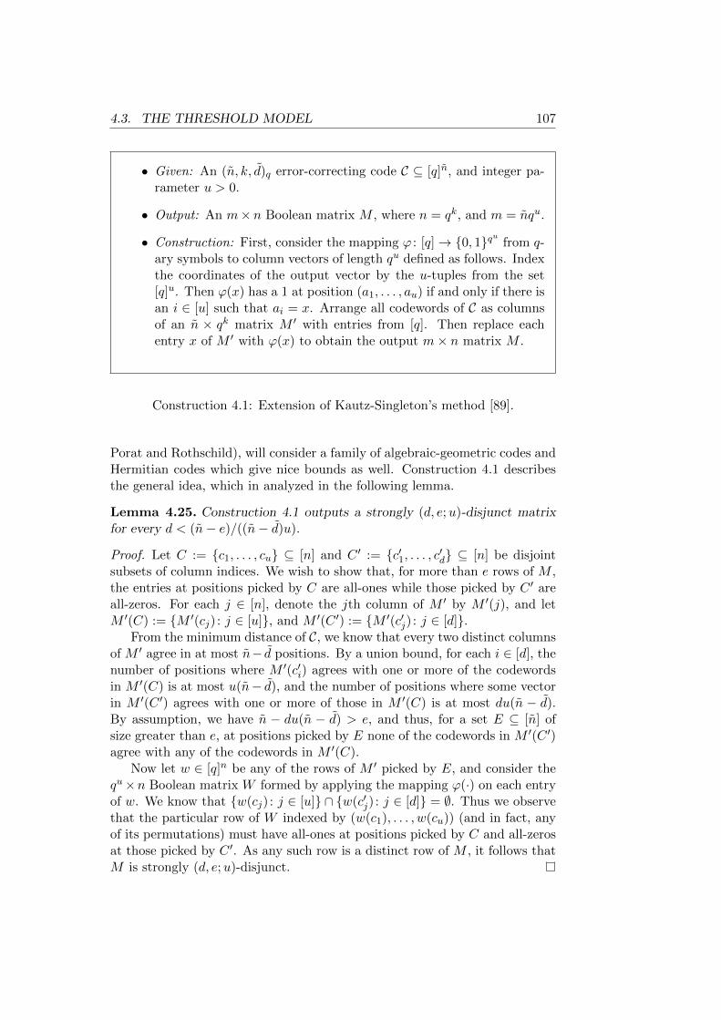
4.3. THE THRESHOLD MODEL 107
• Given: An (n, k, d)q error-correcting code C ⊆ [q]n, and integer pa-rameter u > 0.
• Output: An m× n Boolean matrix M , where n = qk, and m = nqu.
• Construction: First, consider the mapping ϕ : [q]→ 0, 1qu from q-ary symbols to column vectors of length qu defined as follows. Indexthe coordinates of the output vector by the u-tuples from the set[q]u. Then ϕ(x) has a 1 at position (a1, . . . , au) if and only if there isan i ∈ [u] such that ai = x. Arrange all codewords of C as columnsof an n × qk matrix M ′ with entries from [q]. Then replace eachentry x of M ′ with ϕ(x) to obtain the output m× n matrix M .
Construction 4.1: Extension of Kautz-Singleton’s method [89].
Porat and Rothschild), will consider a family of algebraic-geometric codes andHermitian codes which give nice bounds as well. Construction 4.1 describesthe general idea, which in analyzed in the following lemma.
Lemma 4.25. Construction 4.1 outputs a strongly (d, e;u)-disjunct matrixfor every d < (n− e)/((n− d)u).
Proof. Let C := c1, . . . , cu ⊆ [n] and C ′ := c′1, . . . , c′d ⊆ [n] be disjointsubsets of column indices. We wish to show that, for more than e rows of M ,the entries at positions picked by C are all-ones while those picked by C ′ areall-zeros. For each j ∈ [n], denote the jth column of M ′ by M ′(j), and letM ′(C) := M ′(cj) : j ∈ [u], and M ′(C ′) := M ′(c′j) : j ∈ [d].
From the minimum distance of C, we know that every two distinct columnsof M ′ agree in at most n− d positions. By a union bound, for each i ∈ [d], thenumber of positions where M ′(c′i) agrees with one or more of the codewordsin M ′(C) is at most u(n− d), and the number of positions where some vectorin M ′(C ′) agrees with one or more of those in M ′(C) is at most du(n − d).By assumption, we have n − du(n − d) > e, and thus, for a set E ⊆ [n] ofsize greater than e, at positions picked by E none of the codewords in M ′(C ′)agree with any of the codewords in M ′(C).
Now let w ∈ [q]n be any of the rows of M ′ picked by E, and consider thequ×n Boolean matrix W formed by applying the mapping ϕ(·) on each entryof w. We know that w(cj) : j ∈ [u] ∩ w(c′j) : j ∈ [d] = ∅. Thus we observethat the particular row of W indexed by (w(c1), . . . , w(cu)) (and in fact, anyof its permutations) must have all-ones at positions picked by C and all-zerosat those picked by C ′. As any such row is a distinct row of M , it follows thatM is strongly (d, e;u)-disjunct.
108 CHAPTER 4. GROUP TESTING
Now we mention a few specific instantiations of the above construction.We will first consider the family of Reed-Solomon codes, that are also usedin the original work of Kautz and Singleton [89], and then move on to thefamily of algebraic geometric (AG) codes on the Tsfasman-Vladut-Zink (TVZ)bound, and Hermitian codes, and finally, codes on the Gilbert-Varshamov(GV) bound. A quick review of the necessary background on coding-theoreticterms is given in Appendix A.
Reed-Solomon Codes
Let p ∈ [0, 1) be an arbitrary “noise” parameter. If we take C to be an [n, k, d]nReed-Solomon code over an alphabet of size n (more precisely, the smallestprime power that is no less than n), where d = n − k + 1, we get a stronglydisjunct (d, e;u)-matrix with
m = O(du log n/(1− p))u+1
rows ande = pn = Ω(pdu(log n)/(1− p)).
AG Codes on the TVZ Bound
Another interesting family for the code C is the family of algebraic geometriccodes that attain the Tsfasman-Vladut-Zink bound (cf. [67,154]). This familyis defined over any alphabet size q ≥ 49 that is a square prime power, andachieves a minimum distance d ≥ n − k − n/(√q − 1). Let e := pn, for anoise parameter p ∈ [0, 1). By Lemma 4.25, the underlying code C needsto have minimum distance at least n(1 − (1 − p)/(du)). Thus in order tobe able to use the above-mentioned family of AG codes, we need to haveq (du/(1 − p))2 =: q0. Let us take an appropriate q ∈ [2q0, 8q0], andfollowing Lemma 4.25, n − d = dn(1 − p)/(du)e. Thus the dimension of Cbecomes at least
k ≥ n− d− n√q − 1
= Ω
(n(1− p)du
)= Ω(n/
√q0),
and subsequently14 we get that log n = k log q ≥ k = Ω(n/√q0). Now, noting
that m = qun, we conclude that
m = qun = O(qu+1/20 log n) = O
(du
1− p
)2u+1
log n,
and e = Ω(pdu(log n)/(1− p)).14Note that, given the parameters p, d, n, the choice of q depends on p, d, as explained
above, and then one can choose the code length n to be the smallest integer for which wehave qk ≥ n. But for the sake of clarity we have assumed that qk = n.
4.3. THE THRESHOLD MODEL 109
We see that the dependence of the number of measurements on the sparsityparameter d is worse for AG codes than Reed-Solomon codes by a factor du,but the construction from AG codes benefits from a linear dependence on log n,compared to logu+1 n for Reed-Solomon codes. Thus, AG codes become morefavorable only when the sparsity is substantially low; namely, when d log n.
Hermitian Codes
A particularly nice family of AG codes arises from the Hermitian functionfield15. Let q′ be a prime power and q := q′2. Then the Hermitian functionfield over Fq is a finite extension of the rational function field Fq(x), denotedby Fq(x, y), where we have yq
′+y = xq
′+1. The structure of this function fieldis relatively well understood and the family of Goppa codes defined over therational points of the Hermitian function field is known as Hermitian codes.This family is recently used by Ben-Aroya and Ta-Shma [10] for constructionof small-bias sets. Below we quote some parameters of Hermitian codes fromtheir work.
The number of rational points of the Hermitian function field is equal toq′3 + 1, which includes a common pole Q∞ of x and y. The genus of thefunction field is g = q′(q′ − 1)/2. For some integer parameter r, we takeG := rQ∞ as the divisor defining the Riemann-Roch space L(G) of the codeC, and the set of rational points except Q∞ as the evaluation points of thecode. Thus the length of C becomes n = q′3. Moreover, the minimum distanceof the code is d = n − deg(G) = n − r. When r ≥ 2g − 1, the dimension ofthe code is given by the Riemann-Roch theorem, which is equal to r − g + 1.For the low-degree regime where r < 2g − 1, the dimension k of the code isthe size of the Wirestrauss semigroup of G, which turns out to be the setW = (i, j) ∈ N2 : j ≤ q′ − 1 ∧ iq′ + j(q′ + 1) ≤ r.
Now, given parameters d, p of the disjunct matrix, define ρ := (1−p)/((d+1)u), take the alphabet size q as a square prime power, and set r := ρq3/2.First we consider the case where r < 2g − 1 = 2q − 2
√q − 1. In this case,
the dimension of the Hermitian code becomes k = |W | = Ω(r2/q) = Ω(ρ2q2).The distance d of the code satisfies d = n − r ≥ n(1 − ρ) and thus, fore := pn, conditions of Lemma 4.25 are satisfied. The number of the rows ofthe resulting measurement matrix becomes m = qu+3/2, and we have n = qk.Therefore,
log n = k log q ≥ k = Ω(ρ2q2)
⇒ q = O(√
log n/ρ)⇒ m = O
((d√log n
1− p)u+3/2
),
and in order to ensure that r < 2g− 1, we need to have du/(1− p) √log n.On the other hand, when du/(1 − p) √log n, we are in the high-degree
15See [142] for an extensive treatment of the notions in algebraic geometry.
110 CHAPTER 4. GROUP TESTING
regime, in which case the dimension of the code becomes k = r − g + 1 =Ω(r) = Ω(ρq3/2), and we will thus have
q = O((log n/ρ)2/3)⇒ m = O
((d log n
1− p)1+2u/3
)Altogether, we conclude that Construction 4.1 with Hermitian codes resultsin a strongly (d, e;u)-disjunct matrix with
m = O
((d√log n
1− p +(d log n
1− p)2/3)u+3/2
)rows, where e = p · Ω
(d(log n)/(1− p) + (d
√log n/(1− p))3/2
). Compared
to the Reed-Solomon codes, the number of measurements has a slightly worsedependence on d, but a much better dependence on n. Compared to AG codeson the TVZ bound, the dependence on d is better while the dependence on nis inferior.
Codes on the GV Bound
A q-ary (n, k, d)-code (of sufficiently large length) is said to be on the Gilbert-Varshamov bound if it satisfies k ≥ n(1 − hq(d/n)), where hq(·) is the q-aryentropy function defined as
hq(x) := x logq(q − 1)− x logq(x)− (1− x) logq(1− x).
It is well known that a random linear code achieves the bound with over-whelming probability (cf. [103]). Now we apply Lemma 4.25 on a code on theGV bound, and calculate the resulting parameters. Let ρ := (1 − p)/(4du),choose any alphabet size q ∈ [1/ρ, 2/ρ], and let C be any q-ary code of lengthn on the GV bound, with minimum distance d ≥ n(1 − 2/q). By the Taylorexpansion of the function hq(x) around x = 1 − 1/q, we see that the dimen-sion of C asymptotically behaves as k = Θ(n/(q log q)). Thus the number ofcolumns of the resulting measurement matrix becomes n = qk = 2Ω(n/q), andtherefore, the number m of its rows becomes
m = qun = O(qu+1 log n) = O((d/(1− p))u+1 log n),
and the matrix would be strongly (d, e;u)-disjunct for
e = pn = Ω(pd(log n)/(1− p)).
We remark that for the range of parameters that we are interested in, Poratand Rothschild [120] have recently come up with a deterministic constructionof linear codes on the GV bound that runs in time poly(qk) (and thus, poly-nomial in the size of the resulting measurement matrix). Their construction
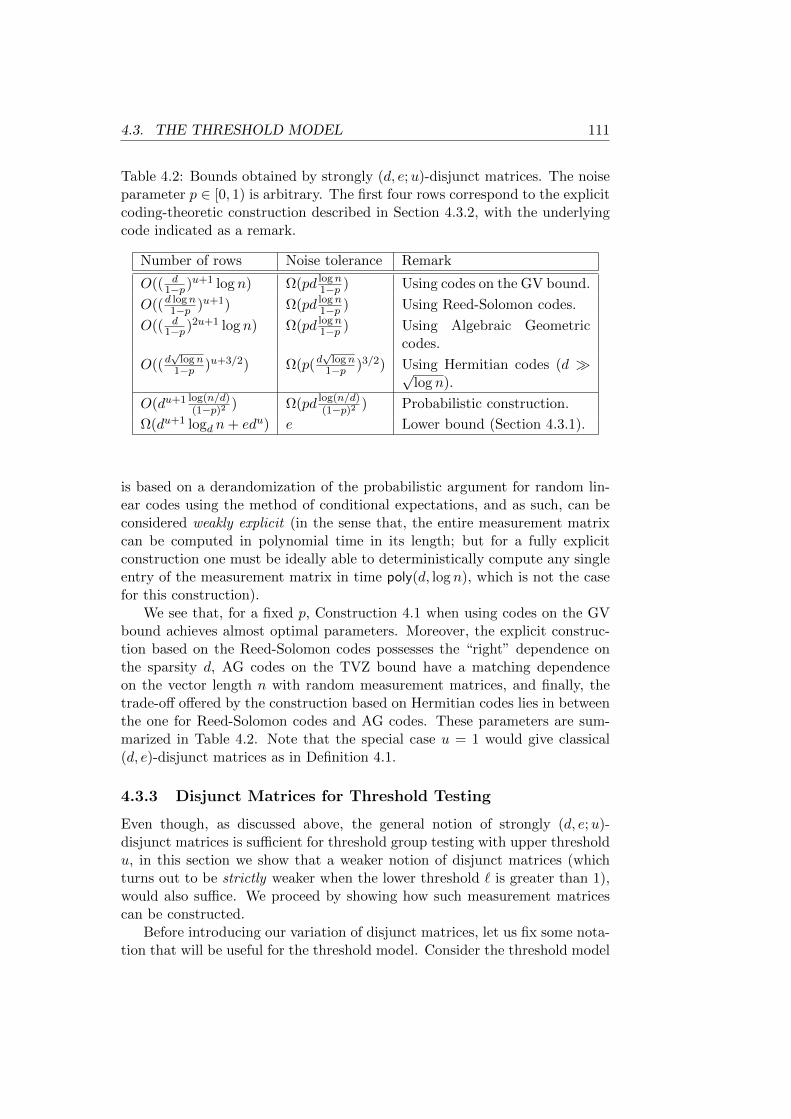
4.3. THE THRESHOLD MODEL 111
Table 4.2: Bounds obtained by strongly (d, e;u)-disjunct matrices. The noiseparameter p ∈ [0, 1) is arbitrary. The first four rows correspond to the explicitcoding-theoretic construction described in Section 4.3.2, with the underlyingcode indicated as a remark.
Number of rows Noise tolerance Remark
O(( d1−p)u+1 log n) Ω(pd logn
1−p ) Using codes on the GV bound.
O((d logn1−p )u+1) Ω(pd logn
1−p ) Using Reed-Solomon codes.
O(( d1−p)2u+1 log n) Ω(pd logn
1−p ) Using Algebraic Geometriccodes.
O((d√
logn1−p )u+3/2) Ω(p(d
√logn
1−p )3/2) Using Hermitian codes (d √log n).
O(du+1 log(n/d)(1−p)2 ) Ω(pd log(n/d)
(1−p)2 ) Probabilistic construction.
Ω(du+1 logd n+ edu) e Lower bound (Section 4.3.1).
is based on a derandomization of the probabilistic argument for random lin-ear codes using the method of conditional expectations, and as such, can beconsidered weakly explicit (in the sense that, the entire measurement matrixcan be computed in polynomial time in its length; but for a fully explicitconstruction one must be ideally able to deterministically compute any singleentry of the measurement matrix in time poly(d, log n), which is not the casefor this construction).
We see that, for a fixed p, Construction 4.1 when using codes on the GVbound achieves almost optimal parameters. Moreover, the explicit construc-tion based on the Reed-Solomon codes possesses the “right” dependence onthe sparsity d, AG codes on the TVZ bound have a matching dependenceon the vector length n with random measurement matrices, and finally, thetrade-off offered by the construction based on Hermitian codes lies in betweenthe one for Reed-Solomon codes and AG codes. These parameters are sum-marized in Table 4.2. Note that the special case u = 1 would give classical(d, e)-disjunct matrices as in Definition 4.1.
4.3.3 Disjunct Matrices for Threshold Testing
Even though, as discussed above, the general notion of strongly (d, e;u)-disjunct matrices is sufficient for threshold group testing with upper thresholdu, in this section we show that a weaker notion of disjunct matrices (whichturns out to be strictly weaker when the lower threshold ` is greater than 1),would also suffice. We proceed by showing how such measurement matricescan be constructed.
Before introducing our variation of disjunct matrices, let us fix some nota-tion that will be useful for the threshold model. Consider the threshold model
112 CHAPTER 4. GROUP TESTING
with thresholds ` and u, and an m × n measurement matrix M that definesthe set of measurements. For a vector x ∈ 0, 1n, denote by M [x]`,u the setof vectors in 0, 1m that correctly encode the measurement outcomes corre-sponding to the vector x. In particular, for any y ∈M [x]`,u we have y(i) = 1if |supp(Mj) ∩ supp(x)| ≥ u, and y(i) = 0 if |supp(Mj) ∩ supp(x)| < `, whereMj indicates the jth row of M . In the gap-free case, the set M [x]`,u may onlyhave a single element that we denote by M [x]u. Note that the gap-free casewith u = 1 reduces to ordinary group testing, and thus we have M [x]1 = M [x].
To make the main ideas more transparent, until Section 4.3.3.3 we willfocus on the gap-free case where ` = u. The extension to nonzero gaps isstraightforward and will be discussed in Section 4.3.3.3. Moreover, often wewill implicitly assume that the Hamming weight of the Boolean vector that isto be identified is at least u (since otherwise, any (u− 1)-sparse vector wouldbe confused with the all-zeros vector). Moreover, we will take the thresholds`, u as fixed constants while the parameters d and n are allowed to grow.
4.3.3.1 The Definition and Properties
Our variation of disjunct matrices along with an “auxiliary” notion of regularmatrices is defined in the following.
Definition 4.26. A Boolean matrix M with n columns is called (d, e;u)-regular if for every subset of columns S ⊆ [n] (called the critical set) andevery Z ⊆ [n] (called the zero set) such that u ≤ |S| ≤ d, |Z| ≤ |S|, S∩Z = ∅,there are more than e rows of M at which M |S has weight exactly u and (atthe same rows) M |Z has weight zero. Any such row is said to u-satisfy S andZ.
If, in addition, for every distinguished column i ∈ S, more than e rows ofM both u-satisfy S and Z and have a 1 at the ith column, the matrix is called(d, e;u)-disjunct (and the corresponding “good” rows are said to u-satisfy i,S, and Z).
It is easy to verify that (assuming 2d ≤ n) the classical notion of (2d−1, e)-disjunct matrices is equivalent to strongly (2d− 1, e; 1)-disjunct and (d, e; 1)-disjunct. Moreover, any (d, e;u)-disjunct matrix is (d, e;u)-regular, (d−1, e;u−1)-regular, and (d, e)-disjunct (but the reverse implications do not in generalhold). Therefore, the lower bound
m = Ω(d2 logd n+ ed)
that applies for (d, e)-disjunct matrices holds for (d, e;u)-disjunct matrices aswell.
Below we show that our notion of disjunct matrices is necessary and suf-ficient for the purpose of threshold group testing:
4.3. THE THRESHOLD MODEL 113
Lemma 4.27. Let M be an m × n Boolean matrix that is (d, e;u)-disjunct.Then for every distinct d-sparse vectors x, x′ ∈ 0, 1n such that16 supp(x) *supp(x′), wgt(x) ≥ |supp(x′) \ supp(x)| and wgt(x) ≥ u, we have
(4.5) |supp(M [x]u) \ supp(M [x′]u)| > e.
Conversely, assuming d ≥ 2u, if M satisfies (4.5) for every choice of x and x′
as above, it must be (bd/2c, e;u)-disjunct.
Proof. First, suppose that M is (d, e;u)-disjunct, and let y := M [x]u andy′ := M [x′]u. Take any i ∈ supp(x) \ supp(x′), and let S := supp(x) andZ := supp(x′) \ supp(x). Note that |S| ≤ d and by assumption, we have|Z| ≤ |S|. Now, Definition 4.26 implies that there is a set E of more than erows of M that u-satisfy i as the distinguished column, S as the critical setand Z as the zero set. Thus for every j ∈ E, the jth row of M restricted tothe columns chosen by supp(x) must have weight exactly u, while its weighton supp(x′) is less than u. Therefore, y(j) = 1 and y′(j) = 0 for more than echoices of j.
For the converse, consider any choice of a distinguished column i ∈ [n], acritical set S ⊆ [n] containing i (such that |S| ≥ u), and a zero set Z ⊆ [n]where |Z| ≤ |S|. Define d-sparse Boolean vectors x, x′ ∈ 0, 1n so thatsupp(x) := S and supp(x′) := S ∪ Z \ i. Let y := M [x]u and y′ := M [x′]uand E := supp(y) \ supp(y′). By assumption we know that |E| > e. Take anyj ∈ E. Since y(j) = 1 and y′(j) = 0, we get that the jth row of M restrictedto the columns picked by S ∪Z \ i must have weight at most u− 1, whereasit must have weight at least u when restricted to S. As the sets i, S \ i,and Z are disjoint, this can hold only if M [j, i] = 1, and moreover, the jthrow of M restricted to the columns picked by S (resp., Z) has weight exactlyu (resp., zero). Hence, this row (as well as all the rows of M picked by E)must u-satisfy i, S, and Z, confirming that M is (bd/2c, e;u)-disjunct.
We will use regular matrices as intermediate building blocks in our con-structions of disjunct matrices to follow. The connection with disjunct ma-trices is made apparent through a direct product of matrices defined in Con-struction 4.2. Intuitively, using this product, regular matrices can be usedto transform any measurement matrix suitable for the standard group test-ing model to one with comparable properties in the threshold model. Thefollowing lemma formalizes this idea.
Lemma 4.28. Let M1 and M2 be Boolean matrices with n columns, suchthat M1 is (d− 1, e1;u− 1)-regular. Let M := M1M2, and suppose that ford-sparse Boolean vectors x, x′ ∈ 0, 1n such that wgt(x) ≥ wgt(x′), we have
|supp(M2[x]1) \ supp(M2[x′]1)| ≥ e2.
16 Note that at least one of the two possible orderings of any two distinct d-sparse vectors,at least one having weight u or more, satisfies this condition.
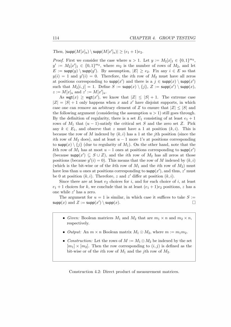
114 CHAPTER 4. GROUP TESTING
Then, |supp(M [x]u) \ supp(M [x′]u)| ≥ (e1 + 1)e2.
Proof. First we consider the case where u > 1. Let y := M2[x]1 ∈ 0, 1m2 ,y′ := M2[x′]1 ∈ 0, 1m2 , where m2 is the number of rows of M2, and letE := supp(y) \ supp(y′). By assumption, |E| ≥ e2. Fix any i ∈ E so thaty(i) = 1 and y′(i) = 0. Therefore, the ith row of M2 must have all zerosat positions corresponding to supp(x′) and there is a j ∈ supp(x) \ supp(x′)such that M2[i, j] = 1. Define S := supp(x) \ j, Z := supp(x′) \ supp(x),z := M [x]u and z′ := M [x′]u.
As wgt(x) ≥ wgt(x′), we know that |Z| ≤ |S| + 1. The extreme case|Z| = |S| + 1 only happens when x and x′ have disjoint supports, in whichcase one can remove an arbitrary element of Z to ensure that |Z| ≤ |S| andthe following argument (considering the assumption u > 1) still goes through.By the definition of regularity, there is a set E1 consisting of at least e1 + 1rows of M1 that (u − 1)-satisfy the critical set S and the zero set Z. Pickany k ∈ E1, and observe that z must have a 1 at position (k, i). This isbecause the row of M indexed by (k, i) has a 1 at the jth position (since theith row of M2 does), and at least u − 1 more 1’s at positions correspondingto supp(x) \ j (due to regularity of M1). On the other hand, note that thekth row of M1 has at most u− 1 ones at positions corresponding to supp(x′)(because supp(x′) ⊆ S ∪ Z), and the ith row of M2 has all zeros at thosepositions (because y′(i) = 0). This means that the row of M indexed by (k, i)(which is the bit-wise or of the kth row of M1 and the ith row of M2) musthave less than u ones at positions corresponding to supp(x′), and thus, z′ mustbe 0 at position (k, i). Therefore, z and z′ differ at position (k, i).
Since there are at least e2 choices for i, and for each choice of i, at leaste1 + 1 choices for k, we conclude that in at least (e1 + 1)e2 positions, z has aone while z′ has a zero.
The argument for u = 1 is similar, in which case it suffices to take S :=supp(x) and Z := supp(x′) \ supp(x).
• Given: Boolean matrices M1 and M2 that are m1 × n and m2 × n,respectively.
• Output: An m× n Boolean matrix M1 M2, where m := m1m2.
• Construction: Let the rows of M := M1M2 be indexed by the set[m1] × [m2]. Then the row corresponding to (i, j) is defined as thebit-wise or of the ith row of M1 and the jth row of M2.
Construction 4.2: Direct product of measurement matrices.
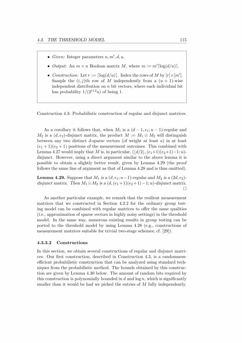
4.3. THE THRESHOLD MODEL 115
• Given: Integer parameters n,m′, d, u.
• Output: An m× n Boolean matrix M , where m := m′dlog(d/u)e.
• Construction: Let r := dlog(d/u)e. Index the rows of M by [r]×[m′].Sample the (i, j)th row of M independently from a (u + 1)-wiseindependent distribution on n bit vectors, where each individual bithas probability 1/(2i+2u) of being 1.
Construction 4.3: Probabilistic construction of regular and disjunct matrices.
As a corollary it follows that, when M1 is a (d − 1, e1;u − 1)-regular andM2 is a (d, e2)-disjunct matrix, the product M := M1 M2 will distinguishbetween any two distinct d-sparse vectors (of weight at least u) in at least(e1 + 1)(e2 + 1) positions of the measurement outcomes. This combined withLemma 4.27 would imply thatM is, in particular, (bd/2c, (e1+1)(e2+1)−1;u)-disjunct. However, using a direct argument similar to the above lemma it ispossible to obtain a slightly better result, given by Lemma 4.29 (the prooffollows the same line of argument as that of Lemma 4.28 and is thus omitted).
Lemma 4.29. Suppose that M1 is a (d, e1;u−1)-regular and M2 is a (2d, e2)-disjunct matrix. Then M1M2 is a (d, (e1 +1)(e2 +1)−1;u)-disjunct matrix.
As another particular example, we remark that the resilient measurementmatrices that we constructed in Section 4.2.2 for the ordinary group test-ing model can be combined with regular matrices to offer the same qualities(i.e., approximation of sparse vectors in highly noisy settings) in the thresholdmodel. In the same way, numerous existing results in group testing can beported to the threshold model by using Lemma 4.28 (e.g., constructions ofmeasurement matrices suitable for trivial two-stage schemes; cf. [29]).
4.3.3.2 Constructions
In this section, we obtain several constructions of regular and disjunct matri-ces. Our first construction, described in Construction 4.3, is a randomness-efficient probabilistic construction that can be analyzed using standard tech-niques from the probabilistic method. The bounds obtained by this construc-tion are given by Lemma 4.30 below. The amount of random bits required bythis construction is polynomially bounded in d and log n, which is significantlysmaller than it would be had we picked the entries of M fully independently.
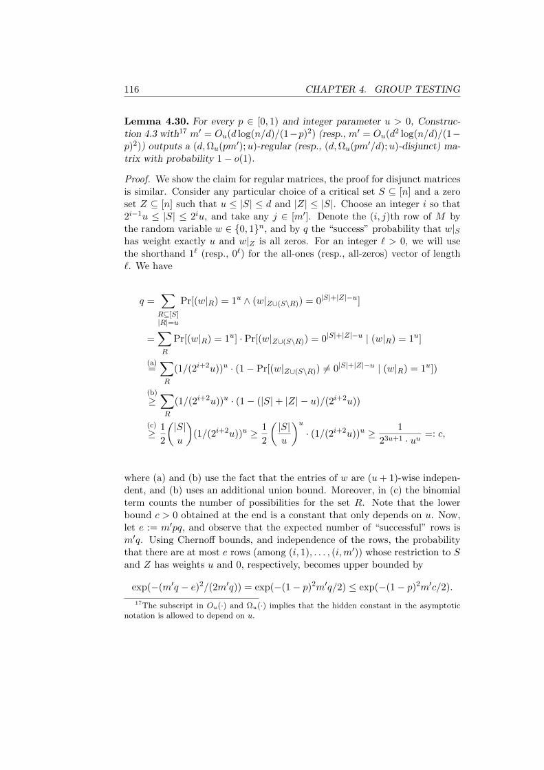
116 CHAPTER 4. GROUP TESTING
Lemma 4.30. For every p ∈ [0, 1) and integer parameter u > 0, Construc-tion 4.3 with17 m′ = Ou(d log(n/d)/(1−p)2) (resp., m′ = Ou(d2 log(n/d)/(1−p)2)) outputs a (d,Ωu(pm′);u)-regular (resp., (d,Ωu(pm′/d);u)-disjunct) ma-trix with probability 1− o(1).
Proof. We show the claim for regular matrices, the proof for disjunct matricesis similar. Consider any particular choice of a critical set S ⊆ [n] and a zeroset Z ⊆ [n] such that u ≤ |S| ≤ d and |Z| ≤ |S|. Choose an integer i so that2i−1u ≤ |S| ≤ 2iu, and take any j ∈ [m′]. Denote the (i, j)th row of M bythe random variable w ∈ 0, 1n, and by q the “success” probability that w|Shas weight exactly u and w|Z is all zeros. For an integer ` > 0, we will usethe shorthand 1` (resp., 0`) for the all-ones (resp., all-zeros) vector of length`. We have
q =∑R⊆[S]|R|=u
Pr[(w|R) = 1u ∧ (w|Z∪(S\R)) = 0|S|+|Z|−u]
=∑R
Pr[(w|R) = 1u] · Pr[(w|Z∪(S\R)) = 0|S|+|Z|−u | (w|R) = 1u]
(a)=∑R
(1/(2i+2u))u · (1− Pr[(w|Z∪(S\R)) 6= 0|S|+|Z|−u | (w|R) = 1u])
(b)
≥∑R
(1/(2i+2u))u · (1− (|S|+ |Z| − u)/(2i+2u))
(c)
≥ 1
2
(|S|u
)(1/(2i+2u))u ≥ 1
2
( |S|u
)u· (1/(2i+2u))u ≥ 1
23u+1 · uu =: c,
where (a) and (b) use the fact that the entries of w are (u+ 1)-wise indepen-dent, and (b) uses an additional union bound. Moreover, in (c) the binomialterm counts the number of possibilities for the set R. Note that the lowerbound c > 0 obtained at the end is a constant that only depends on u. Now,let e := m′pq, and observe that the expected number of “successful” rows ism′q. Using Chernoff bounds, and independence of the rows, the probabilitythat there are at most e rows (among (i, 1), . . . , (i,m′)) whose restriction to Sand Z has weights u and 0, respectively, becomes upper bounded by
exp(−(m′q − e)2/(2m′q)) = exp(−(1− p)2m′q/2) ≤ exp(−(1− p)2m′c/2).
17The subscript in Ou(·) and Ωu(·) implies that the hidden constant in the asymptoticnotation is allowed to depend on u.
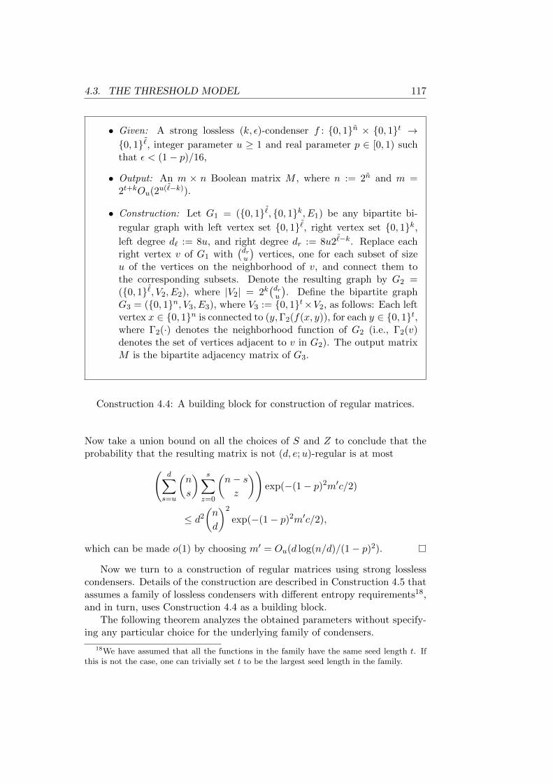
4.3. THE THRESHOLD MODEL 117
• Given: A strong lossless (k, ε)-condenser f : 0, 1n × 0, 1t →0, 1˜
, integer parameter u ≥ 1 and real parameter p ∈ [0, 1) suchthat ε < (1− p)/16,
• Output: An m × n Boolean matrix M , where n := 2n and m =2t+kOu(2u(˜−k)).
• Construction: Let G1 = (0, 1˜, 0, 1k, E1) be any bipartite bi-
regular graph with left vertex set 0, 1˜, right vertex set 0, 1k,
left degree d` := 8u, and right degree dr := 8u2˜−k. Replace each
right vertex v of G1 with(dru
)vertices, one for each subset of size
u of the vertices on the neighborhood of v, and connect them tothe corresponding subsets. Denote the resulting graph by G2 =(0, 1˜
, V2, E2), where |V2| = 2k(dru
). Define the bipartite graph
G3 = (0, 1n, V3, E3), where V3 := 0, 1t×V2, as follows: Each leftvertex x ∈ 0, 1n is connected to (y,Γ2(f(x, y)), for each y ∈ 0, 1t,where Γ2(·) denotes the neighborhood function of G2 (i.e., Γ2(v)denotes the set of vertices adjacent to v in G2). The output matrixM is the bipartite adjacency matrix of G3.
Construction 4.4: A building block for construction of regular matrices.
Now take a union bound on all the choices of S and Z to conclude that theprobability that the resulting matrix is not (d, e;u)-regular is at most(
d∑s=u
(n
s
) s∑z=0
(n− sz
))exp(−(1− p)2m′c/2)
≤ d2
(n
d
)2
exp(−(1− p)2m′c/2),
which can be made o(1) by choosing m′ = Ou(d log(n/d)/(1− p)2).
Now we turn to a construction of regular matrices using strong losslesscondensers. Details of the construction are described in Construction 4.5 thatassumes a family of lossless condensers with different entropy requirements18,and in turn, uses Construction 4.4 as a building block.
The following theorem analyzes the obtained parameters without specify-ing any particular choice for the underlying family of condensers.
18We have assumed that all the functions in the family have the same seed length t. Ifthis is not the case, one can trivially set t to be the largest seed length in the family.
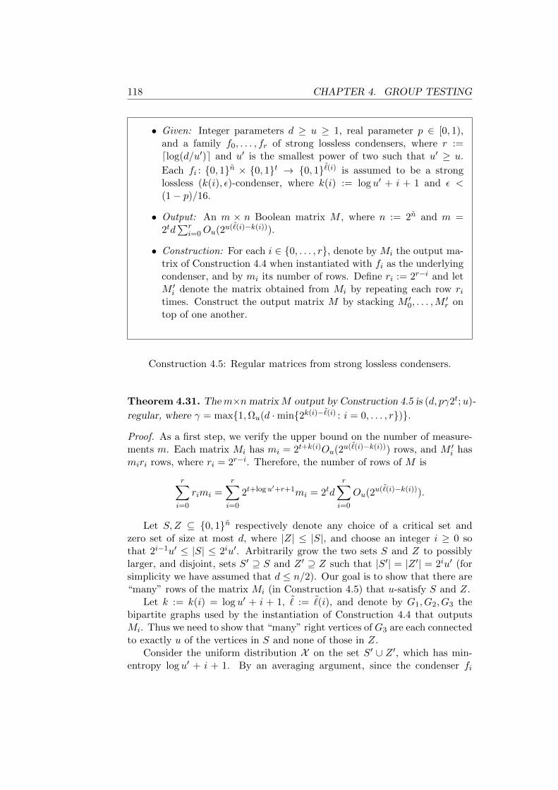
118 CHAPTER 4. GROUP TESTING
• Given: Integer parameters d ≥ u ≥ 1, real parameter p ∈ [0, 1),and a family f0, . . . , fr of strong lossless condensers, where r :=dlog(d/u′)e and u′ is the smallest power of two such that u′ ≥ u.
Each fi : 0, 1n × 0, 1t → 0, 1˜(i) is assumed to be a stronglossless (k(i), ε)-condenser, where k(i) := log u′ + i + 1 and ε <(1− p)/16.
• Output: An m × n Boolean matrix M , where n := 2n and m =2td∑r
i=0Ou(2u(˜(i)−k(i))).
• Construction: For each i ∈ 0, . . . , r, denote by Mi the output ma-trix of Construction 4.4 when instantiated with fi as the underlyingcondenser, and by mi its number of rows. Define ri := 2r−i and letM ′i denote the matrix obtained from Mi by repeating each row ritimes. Construct the output matrix M by stacking M ′0, . . . ,M
′r on
top of one another.
Construction 4.5: Regular matrices from strong lossless condensers.
Theorem 4.31. Them×nmatrixM output by Construction 4.5 is (d, pγ2t;u)-
regular, where γ = max1,Ωu(d ·min2k(i)−˜(i) : i = 0, . . . , r).
Proof. As a first step, we verify the upper bound on the number of measure-ments m. Each matrix Mi has mi = 2t+k(i)Ou(2u(˜(i)−k(i))) rows, and M ′i hasmiri rows, where ri = 2r−i. Therefore, the number of rows of M is
r∑i=0
rimi =
r∑i=0
2t+log u′+r+1mi = 2td
r∑i=0
Ou(2u(˜(i)−k(i))).
Let S,Z ⊆ 0, 1n respectively denote any choice of a critical set andzero set of size at most d, where |Z| ≤ |S|, and choose an integer i ≥ 0 sothat 2i−1u′ ≤ |S| ≤ 2iu′. Arbitrarily grow the two sets S and Z to possiblylarger, and disjoint, sets S′ ⊇ S and Z ′ ⊇ Z such that |S′| = |Z ′| = 2iu′ (forsimplicity we have assumed that d ≤ n/2). Our goal is to show that there are“many” rows of the matrix Mi (in Construction 4.5) that u-satisfy S and Z.
Let k := k(i) = log u′ + i + 1, ˜ := ˜(i), and denote by G1, G2, G3 thebipartite graphs used by the instantiation of Construction 4.4 that outputsMi. Thus we need to show that “many” right vertices of G3 are each connectedto exactly u of the vertices in S and none of those in Z.
Consider the uniform distribution X on the set S′ ∪ Z ′, which has min-entropy log u′ + i + 1. By an averaging argument, since the condenser fi
4.3. THE THRESHOLD MODEL 119
is strong, for more than a p fraction of the choices of the seed y ∈ 0, 1t(call them good seeds), the distribution Zy := fi(X , y) is ε/(1 − p)-close (inparticular, 1/16-close) to a distribution with min-entropy log u′ + i+ 1.
Fix any good seed y ∈ 0, 1t. Let G = (0, 1n, 0, 1˜, E) denote a
bipartite graph representation of fi, where each left vertex x ∈ 0, 1n isconnected to fi(x, y) on the right. Denote by Γy(S
′ ∪Z ′) the right vertices ofG corresponding to the neighborhood of the set of left vertices picked by S′∪Z ′.Note that Γy(S
′ ∪ Z ′) = supp(Zy). Using Proposition 2.14 in the appendix,we see that since Zy is 1/16-close to having min-entropy log(|S′ ∪ Z ′|), thereare at least (7/8)|S′ ∪ Z ′| vertices in Γ(S′ ∪ Z ′) that are each connected toexactly one left vertex in S′ ∪ Z ′. Since |S| ≥ |S′ ∪ Z ′|/4, this implies that atleast |S′ ∪Z ′|/8 vertices in Γ(S′ ∪Z ′) (call them Γ′y) are connected to exactlyone left vertex in S and no other vertex in S′ ∪ Z ′. In particular we get that|Γ′y| ≥ 2k−3.
Now, in G1, let Ty be the set of left vertices corresponding to Γ′y (regardingthe left vertices of G1 in one-to-one correspondence with the right vertices ofG). The number of edges going out of Ty in G1 is d`|Ty| ≥ u2k. Therefore, asthe number of the right vertices of G1 is 2k, there must be at least one rightvertex that is connected to at least u vertices in Ty. Moreover, a countingargument shows that the number of right vertices connected to at least uvertices in Ty is also at least 2k−
˜2k/(10u).
Observe that in construction of G2 from G1, any right vertex of G1 isreplicated
(dru
)times, one for each u-subset of its neighbors. Therefore, for a
right vertex of G1 that is connected to at least u left vertices in Ty, one ormore of its copies in G2 must be connected to exactly u vertex in Ty (amongthe left vertices of G2) and no other vertex (since the right degree of G2 isequal to u).
Define γ′ := max1, 2k−˜2k/(10u). From the previous argument we know
that, looking at Ty as a set of left vertices of G2, there are at least γ′ rightvertices on the neighborhood of Ty in G2 that are connected to exactly u ofthe vertices in Ty and none of the left vertices outside Ty. Letting vy be anysuch vertex, this implies that the vertex (y, vy) ∈ V3 on the right part of G3
is connected to exactly u of the vertices in S, and none of the vertices in Z.Since the argument holds for every good seed y, the number of such vertices isat least the number of good seeds, which is more than pγ′2t. Since the rows ofthe matrix mi are repeated ri = 2r−i times in M , we conclude that M has atleast pγ′2t+r−i ≥ pγ2t rows that u-satisfy S and Z, and the claim follows.
Instantiations
We now instantiate the result obtained in Theorem 4.31 by various choicesof the family of lossless condensers. The crucial factors that influence thenumber of measurements are the seed length and the output length of thecondenser. In particular, we will consider optimal lossless condensers (with
120 CHAPTER 4. GROUP TESTING
parameters achieved by random functions), zig-zag based construction of The-orem 4.19, and the coding-theoretic construction of Guruswami et al., quotedin Theorem 2.22. The results are summarized in the following theorem.
Theorem 4.32. Let u > 0 be fixed, and p ∈ [0, 1) be a real parameter. Thenfor integer parameters d, n ∈ N where u ≤ d ≤ n,
1. Using an optimal lossless condenser in Construction 4.5 results in anm1 × n matrix M1 that is (d, e1;u)-regular, where
m1 = O(d(log n)(log d)/(1− p)u+1)
and e1 = Ω(pd log n),
2. Using the lossless condenser of Theorem 4.19 in Construction 4.5 resultsin an m2 × n matrix M2 that is (d, e2;u)-regular, where
m2 = O(T2d(log d)/(1− p)u)
for some
T2 = exp(O(log3((log n)/(1− p)))) = quasipoly(log n),
and e2 = Ω(pdT2(1− p)).
3. Let β > 0 be any fixed constant. Then Construction 4.5 can be instan-tiated using the lossless condenser of Theorem 2.22 so that we obtain anm3 × n matrix M3 that is (d, e3;u)-regular, where
m3 = O(T 1+u3 d1+β(log d))
forT3 := ((log n)(log d)/(1− p))1+u/β = poly(log n, log d),
and e3 = Ω(pmaxT3, d1−β/u).
Proof. First we show the claim for M1. In this case, we take each fi inConstruction 4.5 to be an optimal lossless condenser satisfying the boundsobtained in19 [23]. Thus we have that 2t = O(n/ε) = O(log n/ε), and for every
i = 0, . . . , r, we have 2˜(i)−k(i) = O(1/ε), where ε = O(1 − p). Now we apply
Theorem 4.31 to obtain the desired bounds (and in particular, γ = Ω(εd)).Similarly, for the construction of M2 we set up each fi using the explicit
construction of condensers in Theorem 4.19 for min-entropy k(i). In this case,the maximum required seed length is t = O(log3(n/ε)), and we let
T2 := 2t = exp(O(log3((log n)/(1− p)))).19This result is similar in spirit to the probabilistic argument used in [122] for showing
the existence of good extractors.
4.3. THE THRESHOLD MODEL 121
Moreover, for every i = 0, . . . , r, we have 2˜(i)−k(i) = O(1/ε). Plugging these
parameters in Theorem 4.31 gives γ = Ω(εd) and the bounds on m2 and e2
follow.Finally, for M3 we use Theorem 2.22 with α := β/u. Thus the maximum
seed length becomes
t = (1 + u/β) log(n(log d)/(1− p)) +O(1),
and for every i = 0, . . . , r, we have ˜(i) − k(i) = O(t + β(log d)/u). Clearly,T3 = Θ(2t), and thus (using Theorem 4.31) the number of measurementsbecomes m3 = T 1+ud1+β(log d). Moreover, we get
γ = max1,Ω(d1−β/u/T ),
which givese3 = Ω(pTγ) = pmaxT, d1−β/u,
as claimed.
By combining this result with Lemma 4.29 using any explicit constructionof classical disjunct matrices, we will obtain (d, e;u)-disjunct matrices thatcan be used in the threshold model with any fixed threshold, sparsity d, anderror tolerance be/2c.
In particular, using the coding-theoretic explicit construction of nearlyoptimal classical disjunct matrices (see Table 4.2), we obtain (d, e;u)-disjunctmatrices with
m = O(m′d2(log n)/(1− p)2)
rows and error tolerance
e = Ω(e′pd(log n)/(1− p)),
where m′ and e′ are respectively the number of rows and error tolerance ofany of the regular matrices obtained in Theorem 4.32.
We note that in all cases, the final dependence on the sparsity parameterd is, roughly, O(d3) which has an exponent independent of the threshold u.Table 4.3 summarizes the obtained parameters for the general case (with ar-bitrary gaps). We see that, when d is not negligibly small (e.g., d = n1/10),the bounds obtained by our explicit constructions are significantly better thanthose offered by strongly disjunct matrices (as in Table 4.2).
4.3.3.3 The Case with Positive Gaps
In preceding sections we have focused on the case where g = 0. However, weobserve that all the techniques that we have developed so far can be extendedto the positive-gap case in a straightforward way. The main observations areas follows.
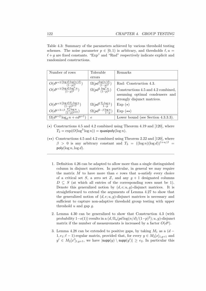
122 CHAPTER 4. GROUP TESTING
Table 4.3: Summary of the parameters achieved by various threshold testingschemes. The noise parameter p ∈ [0, 1) is arbitrary, and thresholds `, u =`+ g are fixed constants. “Exp” and “Rnd” respectively indicate explicit andrandomized constructions.
Number of rows Tolerable Remarkserrors
O(dg+2 (log d) log(n/d)(1−p)2 ) Ω(pd log(n/d)
(1−p)2 ) Rnd: Construction 4.3.
O(dg+3 (log d) log2 n(1−p)2 ) Ω(pd2 log2 n
(1−p)2 ) Constructions 4.5 and 4.2 combined,assuming optimal condensers andstrongly disjunct matrices.
O(dg+3 (log d)T2 logn(1−p)g+2 ) Ω(pd2 T2 logn
1−p ) Exp (?)
O(dg+3+β T `3 logn(1−p)g+2 ) Ω(pd2−β logn
1−p ) Exp (??)
Ω(dg+2 logd n+ edg+1) e Lower bound (see Section 4.3.3.3).
(?) Constructions 4.5 and 4.2 combined using Theorem 4.19 and [120], whereT2 = exp(O(log3 log n)) = quasipoly(log n).
(??) Constructions 4.5 and 4.2 combined using Theorem 2.22 and [120], whereβ > 0 is any arbitrary constant and T3 = ((log n)(log d))1+u/β =poly(log n, log d).
1. Definition 4.26 can be adapted to allow more than a single distinguishedcolumn in disjunct matrices. In particular, in general we may requirethe matrix M to have more than e rows that u-satisfy every choiceof a critical set S, a zero set Z, and any g + 1 designated columnsD ⊆ S (at which all entries of the corresponding rows must be 1).Denote this generalized notion by (d, e;u, g)-disjunct matrices. It isstraightforward to extend the arguments of Lemma 4.27 to show thatthe generalized notion of (d, e;u, g)-disjunct matrices is necessary andsufficient to capture non-adaptive threshold group testing with upperthreshold u and gap g.
2. Lemma 4.30 can be generalized to show that Construction 4.3 (withprobability 1−o(1)) results in a (d,Ωu(pd log(n/d)/(1−p)2);u, g)-disjunctmatrix if the number of measurements is increased by a factor O(dg).
3. Lemma 4.28 can be extended to positive gaps, by taking M1 as a (d −1, e1; `− 1)-regular matrix, provided that, for every y ∈ M2[x]1,g+1 andy′ ∈ M2[x′]1,g+1, we have |supp(y) \ supp(y′)| ≥ e2. In particular this
4.4. NOTES 123
is the case if M2 is strongly (d, e2 − 1; g + 1)-disjunct20. Similarly forLemma 4.29, M2 must be taken as a strongly (2d, e2; g+1)-disjunct ma-trix. Consequently, using the coding-theoretic construction of stronglydisjunct matrices described in Section 4.3.2, our explicit constructionsof (d, e;u)-disjunct matrices can be extended to the gap model at thecost of a factor O(dg) increase in the number of measurements (as sum-marized in Table 4.3).
4. Observe that a (d, e;u, g)-disjunct matrix is in particular, strongly (d−g, e; g+ 1)-disjunct and thus, the lower bound Ω(dg+2 logd n+ edg+1) onthe number of rows of strongly disjunct matrices applies to them as well.
4.4 Notes
The notion of d-disjunct matrices is also known in certain equivalent forms;e.g., d-superimposed codes, d-separable matrices, or d-cover-free families (cf.[50]). The special case of Definition 4.7 corresponding to (0, 0, e′0, 0)-resilientmatrices is related to the notion of selectors in [43] and resolvable matrices in[56]. Lemma 4.10 is similar in spirit to the lower bound obtained in [43] forthe size of selectors.
The notion of strongly disjunct matrices, in its general form, has beenstudied in the literature under different names and equivalent formulations,e.g., superimposed (u, d)-designs/codes and (u, d) cover-free families (see [26,28,53,91,144,145] and the references therein).
4.A Some Technical Details
For a positive integer c > 1, define a c-hypergraph as a tuple (V,E), where Vis the set of vertices and E is the set of hyperedges such that every e ∈ E isa subset of V of size c. The degree of a vertex v ∈ V , denoted by deg(v), isthe size of the set e ∈ E : v ∈ E. Note that |E| ≤
(|V |c
)and deg(v) ≤
( |V |c−1
).
The density of the hypergraph is given by |E|/(|V |c
). A vertex cover on the
hypergraph is a subset of vertices that contains at least one vertex from everyhyperedge. A matching is a set of pairwise disjoint hyperedges. It is wellknown that any dense hypergraph must have a large matching. Below wereconstruct a proof of this claim.
Proposition 4.33. Let H be a c-hypergraph such that every vertex cover ofH has size at least k. Then H has a matching of size at least k/c.
Proof. Let M be a maximal matching of H, i.e., a matching that cannot beextended by adding further hyperedges. Let C be the set of all vertices that
20Here we are also considering the unavoidable assumption thatmax|supp(x) \ supp(x′)|, |supp(x′) \ supp(x)| > g.
124 CHAPTER 4. GROUP TESTING
participate in hyperedges of M . Then C has to be a vertex cover, as otherwiseone could add an uncovered hyperedge to M and violate maximality of M .Hence, c|M | = |C| ≥ k, and the claim follows.
Lemma 4.34. Let H = (V,E) be a c-hypergraph with density at least ε > 0.Then H has a matching of size at least ε
c2(|V | − c+ 1).
Proof. For every subset S ⊆ V of size c, denote by 1(S) the indicator valueof S being in E. Let C be any vertex cover of H. Denote by S the set of allsubsets of V of size c. Then we have
ε
(|V |c
)≤∑S∈S
1(S) ≤∑v∈C
deg(v) ≤ |C|( |V |c− 1
).
Hence, |C| ≥ ε(n− c+ 1)/c, and the claim follows using Proposition 4.33.
Andantino
Frederic Chopin (1810–1849): Ballade Op. 38 No. 2 in F major.

“How is an error possible inmathematics?”
— Henri Poincare
Chapter 5
Capacity Achieving Codes
One of the basic goals of coding theory is coming up with efficient construc-tions of error-correcting codes that allow reliable transmission of informationover discrete communication channels. Already in the seminal work of Shan-non [136], the notion of channel capacity was introduced which is a charac-teristic of the communication channel that determines the maximum rate atwhich reliable transmission of information (i.e., with vanishing error proba-bility) is possible. However, Shannon’s result did not focus on the feasibilityof the underlying code and mainly concerned with the existence of reliable,albeit possibly complex, coding schemes. Here feasibility can refer to a com-bination of several criteria, including: succinct description of the code and itsefficient computability, the existence of an efficient encoder and an efficientdecoder, the error probability, and the set of message lengths for which thecode is defined.
Besides heuristic attempts, there is a large body of rigorous work in theliterature on coding theory with the aim of designing feasible capacity ap-proaching codes for various discrete channels, most notably, the natural andfundamental cases of the binary erasure channel (BEC) and binary symmetricchannel (BSC). Some notable examples in “modern coding” include Turbocodes and sparse graph codes (e.g., LDPC codes and Fountain codes, cf.[13,125,137]). These classes of codes are either known or strongly believed tocontain capacity achieving ensembles for the erasure and symmetric channels.
While such codes are very appealing both theoretically and practically, andare in particular designed with efficient decoding in mind, in this area therestill is a considerable gap between what we can prove and what is evidenced bypractical results, mainly due to complex combinatorial structure of the codeconstructions. Moreover, almost all known code constructions in this areainvolve a considerable amount of randomness, which makes them prone to apossibility of design failure (e.g., choosing an “unfortunate” degree sequence
126
127
for an LDPC code). While the chance of such possibilities is typically small, ingeneral there is no known efficient way to certify whether a particular outcomeof the code construction is satisfactory. Thus, it is desirable to come up withconstructions of provably capacity achieving code families that are explicit,i.e., are efficient and do not involve any randomness.
Explicit construction of capacity achieving codes was considered as earlyas the classic work of Forney [60], who showed that concatenated codes canachieve the capacity of various memoryless channels. In this construction, anouter MDS code is concatenated with an inner code with small block lengththat can be found in reasonable time by brute force search. An importantsubsequent work by Justesen [87] (that was originally aimed for explicit con-struction of asymptotically good codes) shows that it is possible to eliminatethe brute force search by varying the inner code used for encoding differentsymbols of the outer encoding, provided that the ensemble of inner codescontains a large fraction of capacity achieving codes.
Recently, Arikan [7] gave a framework for deterministic construction ofcapacity achieving codes for discrete memoryless channels (DMCs) with bi-nary input that are equipped with efficient encoders and decoders and attainslightly worse than exponentially small error probability. These codes are de-fined for every block length that is a power of two, which might be considereda restrictive requirement. Moreover, the construction is currently explicit (inthe sense of polynomial-time computability of the code description) only forthe special case of BEC and requires exponential time otherwise.
In this chapter, we revisit the concatenation scheme of Justesen and givenew constructions of the underlying ensemble of the inner codes. The codeensemble used in Justesen’s original construction is attributed to Wozencraft.Other ensembles that are known to be useful in this scheme include the en-semble of Goppa codes and shortened cyclic codes (see [127], Chapter 12).The number of codes in these ensembles is exponential in the block lengthand they achieve exponentially small error probability. These ensembles arealso known to achieve the Gilbert-Varshamov bound, and owe their capacityachieving properties to the property that each nonzero vector belongs to asmall number of the codes in the ensemble.
Here, we will use extractors and lossless condensers to construct muchsmaller ensembles with similar, random-like, properties. The quality of theunderlying extractor or condenser determines the quality of the resulting codeensemble. In particular, the size of the code ensemble, the decoding error andproximity to the channel capacity are determined by the seed length, the error,and the output length of the extractor or condenser being used.
As a concrete example, we will instantiate our construction with appro-priate choices of the underlying condenser (or extractor) and obtain, for everyblock length n, a capacity achieving ensemble of size 2n that attains expo-nentially small error probability for both erasure and symmetric channels (aswell as the broader range of channels described above), and an ensemble of
128 CHAPTER 5. CAPACITY ACHIEVING CODES
quasipolynomial1 size 2O(log3 n) that attains the capacity of BEC. Using nearlyoptimal extractors and condensers that require logarithmic seed lengths, it ispossible to obtain polynomially small capacity achieving ensembles for anyblock length.
Finally, we apply our constructions to Justesen’s concatenation scheme toobtain an explicit construction of capacity-achieving codes for both BEC andBSC that attain exponentially small error, as in the original construction ofForney. Moreover, the running time of the encoder is almost linear in the blocklength, and decoding takes almost linear time for BEC and almost quadratictime for BSC. Using our quasipolynomial-sized ensemble as the inner code, weare able to construct a fully explicit code for BEC that is defined and capacityachieving for every choice of the message length.
5.1 Discrete Communication Channels
A discrete communication channel is a randomized process that takes a po-tentially infinite stream of symbols X0, X1, . . . from an input alphabet Σ andoutputs an infinite stream Y0, Y1, . . . from an output alphabet Γ. The indicesintuitively represent the time, and each output symbol is only determinedfrom what channel has observed in the past. More precisely, given X0, . . . , Xt,the output symbol Yt must be independent of Xt+1, Xt+2, . . .. Here we willconcentrate on finite input and finite output channels, that is, the alphabetsΣ and Γ are finite. In this case, the conditional distribution p(Yt|Xt) of eachoutput symbol Yt given the input symbol Xt can be written as a stochastic|Σ| × |Γ| transition matrix, where each row is a probability distribution.
Of particular interest is a memoryless channel, which is intuitively “oblivi-ous” of the past. In this case, the transition matrix is independent of the timeinstance. That is, we have p(Yt|Xt) = p(Y0|X0) for every t. When the rowsof the transition matrix are permutations of one another and so is the casefor the columns, the channel is called symmetric. For example, the channeldefined by
p(Y |X) =
0.4 0.1 0.50.5 0.4 0.10.1 0.5 0.4
is symmetric. Intuitively, a symmetric channel does not “read” the inputsequence. An important class of symmetric channels is defined by additivenoise. In an additive noise channel, the input and output alphabets are thesame finite field Fq and each output symbol Yt is obtained from Xt using
Yt = Xt + Zt,
1A quantity f(n) is said to be quasipolynomial in n (denoted by f(n) = quasipoly(n)) if
f(n) = 2(logn)O(1)
.
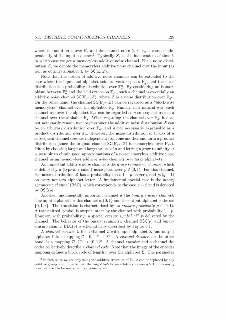
5.1. DISCRETE COMMUNICATION CHANNELS 129
where the addition is over Fq and the channel noise Zt ∈ Fq is chosen inde-pendently of the input sequence2. Typically Zt is also independent of time t,in which case we get a memoryless additive noise channel. For a noise distri-bution Z, we denote the memoryless additive noise channel over the input (aswell as output) alphabet Σ by SC(Σ,Z).
Note that the notion of additive noise channels can be extended to thecase where the input and alphabet sets are vector spaces Fnq , and the noisedistribution is a probability distribution over Fnq . By considering an isomor-phism between Fnq and the field extension Fqn , such a channel is essentially anadditive noise channel SC(Fqn ,Z), where Z is a noise distribution over Fqn .On the other hand, the channel SC(Fqn ,Z) can be regarded as a “block-wisememoryless” channel over the alphabet Fq. Namely, in a natural way, eachchannel use over the alphabet Fqn can be regarded as n subsequent uses of achannel over the alphabet Fq. When regarding the channel over Fq, it doesnot necessarily remain memoryless since the additive noise distribution Z canbe an arbitrary distribution over Fqn and is not necessarily expressible as aproduct distribution over Fq. However, the noise distribution of blocks of nsubsequent channel uses are independent from one another and form a productdistribution (since the original channel SC(Fqn ,Z) is memoryless over Fqn).Often by choosing larger and larger values of n and letting n grow to infinity, itis possible to obtain good approximations of a non-memoryless additive noisechannel using memoryless additive noise channels over large alphabets.
An important additive noise channel is the q-ary symmetric channel , whichis defined by a (typically small) noise parameter p ∈ [0, 1). For this channel,the noise distribution Z has a probability mass 1 − p on zero, and p/(q − 1)on every nonzero alphabet letter. A fundamental special case is the binarysymmetric channel (BSC), which corresponds to the case q = 2 and is denotedby BSC(p).
Another fundamentally important channel is the binary erasure channel .The input alphabet for this channel is 0, 1 and the output alphabet is the set0, 1, ?. The transition is characterized by an erasure probability p ∈ [0, 1).A transmitted symbol is output intact by the channel with probability 1− p.However, with probability p, a special erasure symbol “?” is delivered by thechannel. The behavior of the binary symmetric channel BSC(p) and binaryerasure channel BEC(p) is schematically described by Figure 5.1.
A channel encoder E for a channel C with input alphabet Σ and outputalphabet Γ is a mapping C : 0, 1k → Σn. A channel decoder, on the otherhand, is a mapping D : Γn → 0, 1k. A channel encoder and a channel de-coder collectively describe a channel code. Note that the image of the encodermapping defines a block code of length n over the alphabet Σ. The parameter
2 In fact, since we are only using the additive structure of Fq, it can be replaced by anyadditive group, and in particular, the ring Z/qZ for an arbitrary integer q > 1. This way, qdoes not need to be restricted to a prime power.
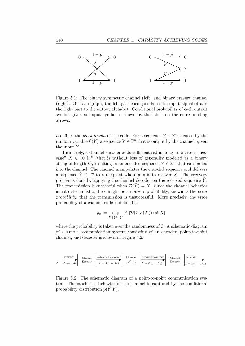
130 CHAPTER 5. CAPACITY ACHIEVING CODES
0
1 1
01− p
1− p
p
p
0
1 1
0
?
1− p
1− p
p
p
Figure 5.1: The binary symmetric channel (left) and binary erasure channel(right). On each graph, the left part corresponds to the input alphabet andthe right part to the output alphabet. Conditional probability of each outputsymbol given an input symbol is shown by the labels on the correspondingarrows.
n defines the block length of the code. For a sequence Y ∈ Σn, denote by therandom variable C(Y ) a sequence Y ∈ Γn that is output by the channel, giventhe input Y .
Intuitively, a channel encoder adds sufficient redundancy to a given “mes-sage” X ∈ 0, 1k (that is without loss of generality modeled as a binarystring of length k), resulting in an encoded sequence Y ∈ Σn that can be fedinto the channel. The channel manipulates the encoded sequence and deliversa sequence Y ∈ Γn to a recipient whose aim is to recover X. The recoveryprocess is done by applying the channel decoder on the received sequence Y .The transmission is successful when D(Y ) = X. Since the channel behavioris not deterministic, there might be a nonzero probability, known as the errorprobability, that the transmission is unsuccessful. More precisely, the errorprobability of a channel code is defined as
pe := supX∈0,1k
Pr[D(C(E(X))) 6= X],
where the probability is taken over the randomness of C. A schematic diagramof a simple communication system consisting of an encoder, point-to-pointchannel, and decoder is shown in Figure 5.2.
ChannelEncoder
X = (X1, . . . ,Xk) Y = (Y1, . . . , Yn)
message redundant encoding received sequence
Y = (Y1, . . . , Yn)
Channel Decoder
Channel
p(Y |Y )
estimate
X = (X1, . . . , Xk)
Figure 5.2: The schematic diagram of a point-to-point communication sys-tem. The stochastic behavior of the channel is captured by the conditionalprobability distribution p(Y |Y ).
5.1. DISCRETE COMMUNICATION CHANNELS 131
For linear codes over additive noise channels, it is often convenient towork with syndrome decoders. Consider a linear code with generator andparity check matrices G and H, respectively. The encoding of a messagex (considered as a row vector) can thus be written as xG. Suppose thatthe encoded sequence is transmitted over an additive noise channel, whichproduces a noisy sequence y := xG+ z, for a randomly chosen z according tothe channel distribution. The receiver receives the sequence y and, withoutloss of generality, the decoder’s task is to obtain an estimate of the noiserealization z from y. Now, observe that
Hy> = HG>x> +Hz> = Hz>,
where the last equality is due to the orthogonality of the generator and par-ity check matrices. Therefore, Hz> is available to the decoder and thus, inorder to decode the received sequence, it suffices to obtain an estimate of thenoise sequence z from the syndrome Hz>. A syndrome decoder is a functionthat, given the syndrome, outputs an estimate of the noise sequence (notethat this is independent of the codeword being sent). The error probability ofa syndrome decoder can be simply defined as the probability (over the noiserandomness) that it obtains an incorrect estimate of the noise sequence. Ob-viously, the error probability of a syndrome decoder upper bounds the errorprobability of the channel code.
The rate of a channel code (in bits per channel use) is defined as thequantity k/n. We call a rate r ≥ 0 feasible if for every ε > 0, there is achannel code with rate r and error probability at most ε. The rate of a channelcode describes its efficiency; the larger the rate, the more information canbe transmitted through the channel in a given “time frame”. A fundamentalquestion is, given a channel C, to find the largest possible rate at which reliabletransmission is possible. In his fundamental work, Shannon [136] introducedthe notion of channel capacity that answers this question. Shannon capacitycan be defined using purely information-theoretic terminology. However, forthe purposes of this chapter, it is more convenient to use the following, more“computational”, definition which turns out to be equivalent to the originalnotion of Shannon capacity:
Cap(C) := supr | r is a feasible rate for the channel C.
Capacity of memoryless symmetric channels has a particularly nice form.Let Z denote the probability distribution defined by any of the rows of thetransition matrix of a memoryless symmetric channel C with output alphabetΓ. Then, capacity of C is given by
Cap(C) = log2 |Γ| −H(Z),
where H(·) denotes the Shannon entropy [40, Section 7.2]. In particular,capacity of the binary symmetric channel BSC(p) (in bits per channel use) is
132 CHAPTER 5. CAPACITY ACHIEVING CODES
equal to1− h(p) = 1 + p log2 p+ (1− p) log2(1− p).
Capacity of the binary erasure channel BEC(p) is moreover known to be 1− p[40, Section 7.1].
A family of channel codes of rate r is an infinite set of channel codes, suchthat for every (typically small) rate loss δ ∈ (0, r) and block length n, thefamily contains a code C(n, δ) of length at least n and rate at least r− δ. Thefamily is called explicit if there is a deterministic algorithm that, given n and δas parameters, computes the encoder function of the code C(n, δ) in polynomialtime in n. For linear channel codes, this is equivalent to computing a generatoror parity check matrix of the code in polynomial time. If, additionally, thealgorithm receives an auxiliary index i ∈ [s], for a size parameter s dependingon n and δ, we instead get an ensemble of size s of codes. An ensemble canbe interpreted as a set of codes of length n and rate at least r − δ each, thatcontains a code for each possibility of the index i.
We call a family of codes capacity achieving for a channel C if the family isof rate Cap(C) and moreover, the code C(n, δ) as described above can be chosento have an arbitrarily small error probability for the channel C. If the errorprobability decays exponentially with the block length n; i.e., pe = O(2−γn),for a constant γ > 0 (possibly depending on the rate loss), then the family issaid to achieve an error exponent γ. We call the family capacity achieving forall lengths if it is capacity achieving and moreover, there is an integer constantn0 (depending only on the rate loss δ) such that for every n ≥ n0, the codeC(n, δ) can be chosen to have length exactly n.
5.2 Codes for the Binary Erasure Channel
Any code with minimum distance d can tolerate up to d − 1 erasures in theworst case3. Thus one way to ensure reliable communication over BEC(p)is to use binary codes with relative minimum distance of about p. However,known negative bounds on the rate-distance trade-off (e.g., the sphere packingand MRRW bounds) do not allow the rate of such codes to approach thecapacity 1 − p. However, by imposing the weaker requirement that most ofthe erasure patterns should be recoverable, it is possible to attain the capacitywith a positive, but arbitrarily small, error probability (as guaranteed by thedefinition of capacity).
In this section, we consider a different relaxation that preserves the worst-case guarantee on the erasure patterns; namely we consider ensembles of linearcodes with the property that any pattern of up to p erasures must be tolerableby all but a negligible fraction of the codes in the ensemble. This in particularallows us to construct ensembles in which all but a negligible fraction of the
3See Appendix A for a quick review of the basic notions in coding theory.
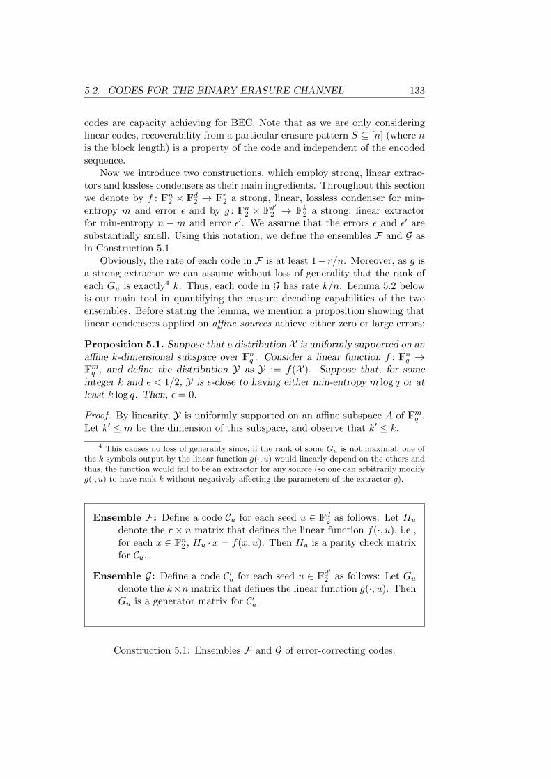
5.2. CODES FOR THE BINARY ERASURE CHANNEL 133
codes are capacity achieving for BEC. Note that as we are only consideringlinear codes, recoverability from a particular erasure pattern S ⊆ [n] (where nis the block length) is a property of the code and independent of the encodedsequence.
Now we introduce two constructions, which employ strong, linear extrac-tors and lossless condensers as their main ingredients. Throughout this sectionwe denote by f : Fn2 × Fd2 → Fr2 a strong, linear, lossless condenser for min-entropy m and error ε and by g : Fn2 × Fd
′2 → Fk2 a strong, linear extractor
for min-entropy n −m and error ε′. We assume that the errors ε and ε′ aresubstantially small. Using this notation, we define the ensembles F and G asin Construction 5.1.
Obviously, the rate of each code in F is at least 1− r/n. Moreover, as g isa strong extractor we can assume without loss of generality that the rank ofeach Gu is exactly4 k. Thus, each code in G has rate k/n. Lemma 5.2 belowis our main tool in quantifying the erasure decoding capabilities of the twoensembles. Before stating the lemma, we mention a proposition showing thatlinear condensers applied on affine sources achieve either zero or large errors:
Proposition 5.1. Suppose that a distribution X is uniformly supported on anaffine k-dimensional subspace over Fnq . Consider a linear function f : Fnq →Fmq , and define the distribution Y as Y := f(X ). Suppose that, for someinteger k and ε < 1/2, Y is ε-close to having either min-entropy m log q or atleast k log q. Then, ε = 0.
Proof. By linearity, Y is uniformly supported on an affine subspace A of Fmq .Let k′ ≤ m be the dimension of this subspace, and observe that k′ ≤ k.
4 This causes no loss of generality since, if the rank of some Gu is not maximal, one ofthe k symbols output by the linear function g(·, u) would linearly depend on the others andthus, the function would fail to be an extractor for any source (so one can arbitrarily modifyg(·, u) to have rank k without negatively affecting the parameters of the extractor g).
Ensemble F : Define a code Cu for each seed u ∈ Fd2 as follows: Let Hu
denote the r × n matrix that defines the linear function f(·, u), i.e.,for each x ∈ Fn2 , Hu · x = f(x, u). Then Hu is a parity check matrixfor Cu.
Ensemble G: Define a code C′u for each seed u ∈ Fd′2 as follows: Let Gudenote the k×n matrix that defines the linear function g(·, u). ThenGu is a generator matrix for C′u.
Construction 5.1: Ensembles F and G of error-correcting codes.
134 CHAPTER 5. CAPACITY ACHIEVING CODES
First, suppose that Y is ε-close to a distribution with min-entropy m log q;i.e., the uniform distribution on Fmq . Now, the statistical distance between Yand the uniform distribution is, by definition,∑
x∈A(q−k
′ − q−m) = 1− qk′−m − 1.
Since ε < 1/4, q ≥ 2, and k′ and m are integers, this implies that the distanceis greater than 1/2 (a contradiction) unless k′ = m, in which case it becomeszero. Therefore, the output distribution is exactly uniform over Fmq .
Now consider the case where Y is ε-close to having min-entropy at leastk log q. Considering that k′ ≤ k, the definition of statistical distance impliesthat ε is at least ∑
x∈A(q−k
′ − q−k) = 1− qk′−k.
Similarly as before, we get that k′ = k, meaning that Y is precisely a distri-bution with min-entropy k log q.
Lemma 5.2. Let S ⊆ [n] be a set of size at most m. Then all but a 5εfraction of the codes in F and all but a 5ε′ fraction of those in G can toleratethe erasure pattern defined by S.
Proof. We prove the result for the ensemble G. The argument for F is similar.Consider a probability distribution S on Fn2 that is uniform on the coordinatesspecified by S := [n] \ S and fixed to zeros elsewhere. Thus the min-entropyof S is at least n − m, and the distribution (U, g(S, U)), where U ∼ Ud′ , isε′-close to Ud′+k.
By Corollary 2.13, for all but a 5ε′ fraction of the choices of u ∈ Fd′2 , thedistribution of g(S, u) is (1/5)-close to Uk. Fix such a u. By Proposition 5.1,the distribution of g(S, u) must in fact be exactly uniform. Thus, the k ×msubmatrix of Gu consisting of the columns picked by S must have rank k,which implies that for every x ∈ Fk2, the projection of the encoding x ·Gu tothe coordinates chosen by S uniquely identifies x.
The lemma combined with a counting argument implies the following corol-lary:
Corollary 5.3. Let S be any distribution on the subsets of [n] of size at mostm. Then all but a
√5ε (resp.,
√5ε′) fraction of the codes in F (resp., G) can
tolerate erasure patterns sampled from S with probability at least 1 −√
5ε(resp., 1−
√5ε′).
Note that the result holds irrespective of the distribution S, contrary tothe familiar case of BEC(p) for which the erasure pattern is an i.i.d. (i.e.,independent and identically-distributed) sequence. For the case of BEC(p),the erasure pattern (regarded as its binary characteristic vector in Fn2 ) is given
5.2. CODES FOR THE BINARY ERASURE CHANNEL 135
by S := (S1, . . . , Sn), where the random variables S1, . . . , Sn ∈ F2 are i.i.d.and Pr[Si = 1] = p. We denote this particular distribution by Bn,p, whichassigns a nonzero probability to every vector in Fn2 . Thus in this case wecannot directly apply Corollary 5.3. However, note that Bn,p can be writtenas a convex combination
(5.1) Bn,p = (1− γ)Un,≤p′ + γD,
for p′ := p + Ω(1) that is arbitrarily close to p, where D is an “error distri-bution” whose contribution γ is exponentially small. The distribution Un,≤p′is the distribution Bn,p conditioned on vectors of weight at most np′. Corol-lary 5.3 applies to Un,≤p′ by setting m = np′. Moreover, by the convex com-bination above, the erasure decoding error probability of any code for erasurepattern distributions Bn,p and Un,≤p′ differ by no more than γ. Therefore, theabove result applied to the erasure distribution Un,≤p′ handles the particularcase of BEC(p) with essentially no change in the error probability.
In light of Corollary 5.3, in order to obtain rates arbitrarily close to thechannel capacity, the output lengths of f and g must be sufficiently close to theentropy requirement m. More precisely, it suffices to have r ≤ (1 + α)m andk ≥ (1−α)m for arbitrarily small constant α > 0. The seed length of f and gdetermine the size of the code ensemble. Moreover, the error of the extractorand condenser determine the erasure error probability of the resulting codeensemble. As achieving the channel capacity is the most important concernfor us, we will need to instantiate f (resp., g) with a linear, strong, losslesscondenser (resp., extractor) whose output length is close to m. We mentionone such instantiation for each function.
For both functions f and g, we can use the explicit extractor and loss-less condenser obtained from the Leftover Hash Lemma (Lemma 2.17), whichis optimal in the output length, but requires a large seed, namely, d = n.The ensemble resulting this way will thus have size 2n, but attains a posi-tive error exponent δ/2 for an arbitrary rate loss δ > 0. Using an optimallossless condenser or extractor with seed length d = log(n) +O(log(1/ε)) andoutput length close to m, it is possible to obtain a polynomially small capacity-achieving ensemble. However, in order to obtain an explicit ensemble of codes,the condenser of extractor being used must be explicit as well.
In the world of linear extractors, we can use Trevisan’s extractor (The-orem 2.20) to improve the size of the ensemble compared to what obtainedfrom the Leftover Hash Lemma. In particular, Trevisan’s extractor combinedwith Corollary 5.3 (using ensemble G) immediately gives the following result:
Corollary 5.4. Let p, c > 0 be arbitrary constants. Then for every integern > 0, there is an explicit ensemble G of linear codes of rate 1 − p − o(1)
such that, the size of G is quasipolynomial, i.e., |G| = 2O(c3 log3 n), and, all butan n−c = o(1) fraction of the codes in the ensemble have error probability atmost n−c when used over BEC(p).
136 CHAPTER 5. CAPACITY ACHIEVING CODES
For the ensemble F , on the other hand, we can use the linear losslesscondenser of Guruswami et al. that only requires a logarithmic seed (Corollary2.23). Using this condenser combined with Corollary 5.3, we can strengthenthe above result as follows:
Corollary 5.5. Let p, c, α > 0 be arbitrary constants. Then for every integern > 0, there is an explicit ensemble F of linear codes of rate 1 − p − α suchthat |G| = O(nc
′) for a constant c′ only depending on c, α. Moreover, all but
an n−c = o(1) fraction of the codes in the ensemble have error probability atmost n−c when used over BEC(p).
5.3 Codes for the Binary Symmetric Channel
The goal of this section is to design capacity achieving code ensembles forthe binary symmetric channel BSC(p). In order to do so, we obtain codes forthe general (and not necessarily memoryless) class SC(Fq,Z) of symmetricchannels, where Z is any flat distribution or sufficiently close to one. Forconcreteness, we will focus on the binary case where q = 2.
Recall that the capacity of BSC(Z), seen as a binary channel, is 1− h(Z)where h(Z) is the entropy rate of Z. The special case BSC(p) is obtained bysetting Z = Bn,p; i.e., the product distribution of n Bernoulli random variableswith probability p of being equal to 1.
The code ensemble that we use for the symmetric channel is the ensembleF , obtained from linear lossless condensers, that we introduced in the pre-ceding section. Thus, we adopt the notation (and parameters) that we usedbefore for defining the ensemble F . Recall that each code in the ensemble hasrate at least 1−r/n. In order to show that the ensemble is capacity achieving,we consider the following brute-force decoder for each code:
Brute-force decoder for code Cu: Given a received word y ∈ Fn2 ,find a codeword y ∈ Fn2 of Cu used and a vector z ∈ supp(Z) suchthat y = y + z. Output y, or an arbitrary codeword if no suchpair is found. If there is more than one choice for the codeword y,arbitrarily choose one of them.
For each u ∈ Fd2, denote by E(Cu,Z) the error probability of the abovedecoder for code Cu over BSC(F2,Z). The following lemma quantifies thisprobability:
Lemma 5.6. Let Z be a flat distribution with entropy m. Then for at leasta 1− 2
√ε fraction of the choices of u ∈ Fd2, we have E(Cu,Z) ≤ √ε.
Proof. The proof is straightforward from the almost-injectivity property oflossless condensers discussed in Section 2.2.2. We will use this property to
5.3. CODES FOR THE BINARY SYMMETRIC CHANNEL 137
construct a syndrome decoder for the code ensemble that achieves a sufficientlysmall error probability.
By Corollary 2.13, for a 1− 2√ε fraction of the choices of u ∈ 0, 1d, the
distribution Y := f(Z, u) is (√ε/2)-close to having min-entropy at least m.
Fix any such u. We show that the error probability E(Cu,Z) is bounded by√ε.
For each y ∈ Fr2, define
N (y) := |x ∈ supp(Z) : f(x, u) = y|
and recall that f(x, u) = Hu ·x. Now suppose that a message is encoded usingthe code Cu to an encoding x ∈ Cu, and that x is transmitted through thechannel. The error probability E(Cu,Z) can be written as
E(Cu,Z) = Prz∼Z
[∃x′ ∈ Cu, ∃z′ ∈ supp(Z) \ z : x+ z = x′ + z′]
≤ Prz∼Z
[∃x′ ∈ Cu, ∃z′ ∈ supp(Z) \ z : Hu · (x+ z) = Hu · (x′ + z′)]
= Prz∼Z
[∃z′ ∈ supp(Z) \ z : Hu · z = Hu · z′](5.2)
= Prz∼Z
[N (H · z) > 1]
= Prz∼Z
[N (f(x, u)) > 1],(5.3)
where (5.2) uses the fact that any codeword of Cu is in the right kernel of Hu.By the first part of Proposition 2.14, there is a set T ⊆ Fr2 of size at least
(1−√ε)|supp(Z)| such that, N (y) = 1 for every y ∈ T . Since Z is uniformlydistributed on its support, this combined with (5.3) immediately implies thatE(Cu,Z) ≤ √ε.
The lemma implies that any linear lossless condenser with entropy require-ment m can be used to construct an ensemble of codes such that all but asmall fraction of the codes are good for reliable transmission over BSC(Z),where Z is an arbitrary flat distribution with entropy at most m. Similar tothe case of BEC, the seed length determines the size of the ensemble, the errorof the condenser bounds the error probability of the decoder, and the outputlength determines the proximity of the rate to the capacity of the channel.Again, using the condenser given by the Leftover Hash Lemma (Lemma 2.17),we can obtain a capacity achieving ensemble of size 2n. Moreover, using thelinear lossless condenser of Guruswami et al. (Corollary 2.23) the ensemblecan be made polynomially small (similar to the result given by Corollary 5.5).
It is not hard to see that the converse of the above result is also true;namely, that any ensemble of linear codes that is universally capacity achievingwith respect to any choice of the noise distribution Z defines a strong linear,lossless, condenser. This is spelled out in the lemma below.
138 CHAPTER 5. CAPACITY ACHIEVING CODES
Lemma 5.7. Let C1, . . . , CT be a binary code ensemble of length n anddimension n − r such that for every flat distribution Z with min-entropy atmost m on Fn2 , all but a γ fraction of the codes in the ensemble (for someγ ∈ [0, 1)) achieve error probability at most ε (under syndrome decoding)when used over SC(Fqn ,Z). Then the function f : Fn2 × [T ]→ Fr2 defined as
f(x, u) := Hu · x,where Hu is a parity check matrix of Cu, is a strong, lossless, (m, 2ε + γ)-condenser.
Proof. The proof is straightforward using similar arguments as in Lemma 5.6.Without loss of generality (by Proposition 2.8), let Z be a flat distributionwith min-entropy m, and denote by D : Fr2 → Fn2 the corresponding syndromedecoder. Moreover, without loss of generality we have taken the decoder to bea deterministic function. For a randomized decoder, one can fix the internalcoin flips so as to preserve the upper bound on its error probability. Now let ube chosen such that Cu achieves an error probability at most ε (we know thisis the case for at least γT of the choices of u).
Denote by T ⊆ supp(Z) the set of noise realizations that can potentiallyconfuse the syndrome decoder. Namely,
T := z ∈ supp(Z) : ∃z′ ∈ supp(Z), z′ 6= z,Hu · z = Hu · z′.Note that, for a random Z ∼ Z, conditioned on the event that Z ∈ T , theprobability that the syndrome decoder errs on Z is at least 1/2, since we knowthat Z can be confused by at least one different noise realization. We can writethis more precisely as
PrZ∼Z
[D(Z) 6= Z | Z ∈ T ] ≥ 1/2.
Since the error probability of the decoder is upper bounded by ε, we concludethat
PrZ∼Z
[Z ∈ T ] ≤ 2ε.
Therefore, the fraction of the elements on support of Z that collide with someother element under the mapping defined by Hu is at most 2ε. Namely,
|Hu · z : z ∈ supp(Z)| ≥ 2m(1− 2ε),
and this is true for at least 1 − γ fraction of the choices of u. Thus, for auniformly random U ∈ [T ] and Z ∼ Z, the distribution of (U,HU · Z) has asupport of size at least
(1− γ)(1− 2ε)T2m ≥ (1− γ − 2ε)T2m.
By the second part of Proposition 2.14, we conclude that this distribution is(2ε+ γ)-close to having entropy m+ log T and thus, the function f defined inthe statement is a strong lossless (m, 2ε+ γ)-condenser.
5.3. CODES FOR THE BINARY SYMMETRIC CHANNEL 139
By this lemma, the known lower bounds on the seed length and the outputlength of lossless condensers that we discussed in Chapter 2 translate into lowerbounds on the size of the code ensemble and proximity to the capacity thatcan be obtained from our framework. In particular, in order to get a positiveerror exponent (i.e., exponentially small error in the block length), the size ofthe ensemble must be exponentially large.
It is worthwhile to point out that the code ensembles F and G discussedin this and the preceding section preserve their erasure and error correctingproperties under any change of basis in the ambient space Fn2 , due to thefact that a change of basis applied on any linear condenser results in a linearcondenser with the same parameters. This is a property achieved by thetrivial, but large, ensemble of codes defined by the set of all r×n parity checkmatrices. Observe that no single code can be universal in this sense, and it isinevitable to have a sufficiently large ensemble to attain this property.
The Case BSC(p)
For the special case of BSC(p), the noise distribution Bn,p is not a flat distri-bution. Fortunately, similar to the BEC case, we can again use convex com-binations to show that the result obtained in Lemma 5.6 can be extended tothis important noise distribution. The main tool that we need is an extensionof Lemma 5.6 to convex combinations with a small number of components.
Suppose that the noise distribution Z is not a flat distribution but can bewritten as a convex combination
(5.4) Z = α1Z1 + · · ·+ αtZt.
of t flat distributions, where the number t of summands is not too large, and
|supp(Z1)| ≥ |supp(Z2)| ≥ · · · ≥ |supp(Zt)|.
For this more general case, we need to slightly tune our brute-force decoderin the way it handles ties. In particular, we now require the decoder to finda codeword y ∈ Cu and a potential noise vector z ∈ supp(Z) that add up tothe received word, as before. However, in case more than one matching pairis found, we will require the decoder to choose the one whose noise vectorz belongs to the component Z1, . . . ,Zt with smallest support (i.e., largestindex). If the noise vector z ∈ supp(Zi) that maximizes the index i is still notunique, the decoder can arbitrarily choose one. Under these conventions, wecan now prove the following:
Lemma 5.8. Suppose that a noise distribution Z is as in (5.4), where eachcomponent Zi has entropy at mostm, and the function f defining the ensembleF is a strong lossless (≤ m+1, ε)-condenser. Then for at least a 1− t(t+1)
√ε
fraction of the choices of u ∈ Fd2, the brute-force decoder satisfies E(Cu,Z) ≤2t√ε.
140 CHAPTER 5. CAPACITY ACHIEVING CODES
Proof. For each 1 ≤ i ≤ j ≤ t, we define a flat distribution Zij that isuniformly supported on supp(Zi) ∪ supp(Zj). Observe that each Zij has min-entropy at most m + 1 and thus the function f is a lossless condenser witherror at most ε for this source. By Corollary 2.13 and a union bound, for a1− t(t+ 1)
√ε fraction of the choices of u ∈ 0, 1d, all t(t+ 1)/2 distributions
f(Zij , u) : 1 ≤ i ≤ j ≤ t
are simultaneously (√ε/2)-close to having min-entropy at least m. Fix any
such u.Consider a random variable Z, representing the channel noise, that is
sampled from Z as follows: First choose an index I ∈ [t] randomly accordingto the distribution induced by (α1, . . . , αt) over the indices, and then samplea random noise Z ∼ ZI . Using the same line of reasoning leading to (5.2)in the proof of Lemma 5.6, the error probability with respect to the code Cu(i.e., the probability that the tuned distance decoder gives a wrong estimateon the noise realization Z) can now be bounded as
E(Cu,Z) ≤ PrI,Z
[∃i ∈ I, . . . , t, ∃z′ ∈ supp(Zi) \ Z : f(Z, u) = f(z′, u)].
For i = 1, . . . , t, denote by Ei the right hand side probability in the abovebound conditioned on the event that I = i. Fix any choice of the index i.Now it suffices to obtain an upper bound on Ei irrespective of the choice of i,since
E(Cu,Z) ≤∑i∈[t]
αiEi.
We call a noise realization z ∈ supp(Zi) confusable if
∃j ≥ i,∃z′ ∈ supp(Zj) \ z : f(z, u) = f(z′, u).
That is, a noise realization is confusable if it can potentially cause the brute-force decoder to compute a wrong noise estimate. Our goal is to obtain anupper bound on the fraction of vectors on supp(Zi) that are confusable.
For each j ≥ i, we know that f(Zij , u) is (√ε/2)-close to having min-
entropy at least m. Therefore, by the first part of Proposition 2.14, the set ofconfusable elements
z ∈ supp(Zi) : ∃z′ ∈ supp(Zj) \ z such that f(z, u) = f(z′, u)
has size at most√ε|supp(Zij)| ≤ 2
√ε|supp(Zi)| (using the fact that, since
j ≥ i, the support of Zj is no larger than that of Zi). By a union bound onthe choices of j, we see that the fraction of confusable elements on supp(Zi)is at most 2t
√ε. Therefore, Ei ≤ 2t
√ε and we get the desired upper bound on
the error probability of the brute-force decoder.
5.4. EXPLICIT CAPACITY ACHIEVING CODES 141
The result obtained by Lemma 5.8 can be applied to the channel BSC(p)by observing that the noise distribution Bn,p can be written as a convex com-bination
Bn,p =
n(p+η)∑i=n(p−η)
αiUn,i + γD,
where Un,i denotes the flat distribution supported on binary vectors of lengthn and Hamming weight exactly i, and D is the distribution Bn,p conditioned onthe vectors whose Hamming weights lie outside the range [n(p− η), n(p+ η)].The parameter η > 0 can be chosen as an arbitrarily small real number, sothat the min-entropies of the distributions Un,i become arbitrarily close to theShannon entropy of Bn,p; namely, nh(p). This can be seen by the estimate(
n
w
)= 2nh(w/n)±o(n),
h(·) being the binary entropy function, that is easily derived from Stirling’sformula. By Chernoff bounds, the error γ can be upper bounded as
γ = PrZ∼Bn,p
[|wgt(Z)− np| > ηn] ≤ 2e−cηnp = 2−Ω(n),
where cη > 0 is a constant only depending on η, and is thus exponentiallysmall. Thus the error probability attained by any code under noise distribu-
tions Bn,p and Z :=∑n(p+η)
i=n(p−η) αiUn,i differ by the exponentially small quan-tity γ. We may now apply Lemma 5.8 on the noise distribution Z to attaincode ensembles for the binary symmetric channel BSC(p). The error prob-ability of the ensemble is at most 2n
√ε, and this bound is satisfied by at
least a 1− n2√ε fraction of the codes. Finally, the code ensemble is capacityachieving for BSC(p) provided that the condenser f attains an output lengthr ≤ (1 + α)(p+ η)n for arbitrarily small constant α, and ε = o(n−4).
5.4 Explicit Capacity Achieving Codes
In the preceding sections, we showed how to obtain small ensembles of explicitcapacity achieving codes for various discrete channels, including the importantspecial cases BEC(p) and BSC(p). Two drawbacks related to these construc-tions are:
1. While an overwhelming fraction of the codes in the ensemble are capacityachieving, in general it is not clear how to pin down a single, capacityachieving code in the ensemble.
2. For the symmetric additive noise channels, the brute-force decoder is ex-tremely inefficient and is of interest only for proving that the constructedensembles are capacity achieving.
142 CHAPTER 5. CAPACITY ACHIEVING CODES
In a classic work, Justesen [87] showed that the idea of code concatenation5
first introduced by Forney [60] can be used to transform any ensemble ofcapacity achieving codes, for a memoryless channel, into an explicit, efficientlydecodable code with improved error probability over the same channel. In thissection we revisit this idea and apply it to our ensembles. For concreteness,we focus on the binary case and consider a memoryless channel C that is eitherBEC(p) or BSC(p).
Throughout this section, we consider an ensemble S of linear codes withblock length n and rate R, for which it is guaranteed that all but a γ = o(1)fraction of the codes are capacity achieving (for a particular DMSC, in ourcase either BEC(p) or BSC(p)) with some vanishing error probability η = o(1)(the asymptotics are considered with respect to the block length n).
Justesen’s concatenated codes take an outer code Cout of block length s :=|S|, alphabet F2k , rate R′ as the outer code. The particular choice of theouter code in the original construction is Reed-Solomon codes. However, wepoint out that any outer code that allows unique decoding of some constantfraction of errors at rates arbitrarily close to one would suffice for the purposeof constructing capacity achieving codes. In particular, in this section wewill use an expander-based construction of asymptotically good codes due toSpielman [141], from which the following theorem can be easily derived6:
Theorem 5.9. For every integer k > 0 and every absolute constant R′ < 1,there is an explicit family of F2-linear codes over F2k for every block lengthand rate R′ that is error-correcting for an Ω(1) fraction of errors. The runningtime of the encoder and the decoder is linear in the bit-length of the codewords.
5.4.1 Justesen’s Concatenation Scheme
The concatenation scheme of Justesen differs from traditional concatenationin that the outer code is concatenated with an ensemble of codes rather thana single inner code.
In this construction, size of the ensemble is taken to be matching with theblock length of the outer code, and each symbol of the outer code is encodedwith one of the inner codes in the ensemble. We use the notation C := Cout Sto denote concatenation of an outer code Cout with the ensemble S of innercodes. Suppose that the alphabet size of the outer code is taken as 2bRnc,where we recall that n and R denote the block length and rate of the innercodes in S.
The encoding of a message with the concatenated code can be obtainedas follows: First, the message is encoded using Cout to obtain an encoding(c1, . . . , cs) ∈ Fs2k , where k = bRnc denotes the dimension of the inner codes.
5 A quick review of code concatenation and its basic properties appears in Appendix A.6There are alternative choices of the outer code that lead to a similar result, e.g.,
expander-based codes due to Guruswami and Indyk [76].
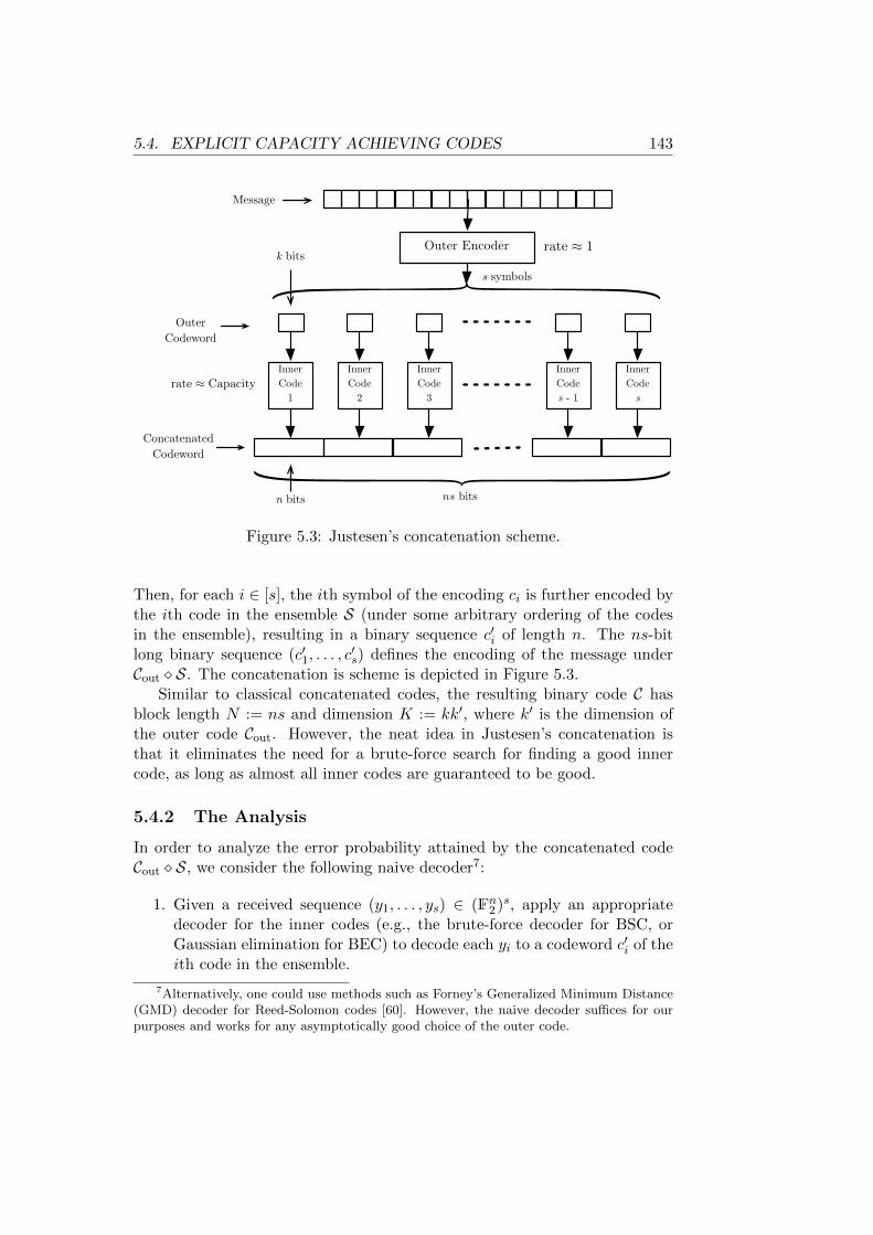
5.4. EXPLICIT CAPACITY ACHIEVING CODES 143
Inner Code
1
Inner Code
2
Inner Code
3
Inner Codes - 1
Inner Code
s
OuterCodeword
Concatenated Codeword
k bitsOuter Encoder
s symbols
Message
n bits ns bits
rate ≈ 1
rate ≈ Capacity
Figure 5.3: Justesen’s concatenation scheme.
Then, for each i ∈ [s], the ith symbol of the encoding ci is further encoded bythe ith code in the ensemble S (under some arbitrary ordering of the codesin the ensemble), resulting in a binary sequence c′i of length n. The ns-bitlong binary sequence (c′1, . . . , c
′s) defines the encoding of the message under
Cout S. The concatenation is scheme is depicted in Figure 5.3.Similar to classical concatenated codes, the resulting binary code C has
block length N := ns and dimension K := kk′, where k′ is the dimension ofthe outer code Cout. However, the neat idea in Justesen’s concatenation isthat it eliminates the need for a brute-force search for finding a good innercode, as long as almost all inner codes are guaranteed to be good.
5.4.2 The Analysis
In order to analyze the error probability attained by the concatenated codeCout S, we consider the following naive decoder7:
1. Given a received sequence (y1, . . . , ys) ∈ (Fn2 )s, apply an appropriatedecoder for the inner codes (e.g., the brute-force decoder for BSC, orGaussian elimination for BEC) to decode each yi to a codeword c′i of theith code in the ensemble.
7Alternatively, one could use methods such as Forney’s Generalized Minimum Distance(GMD) decoder for Reed-Solomon codes [60]. However, the naive decoder suffices for ourpurposes and works for any asymptotically good choice of the outer code.
144 CHAPTER 5. CAPACITY ACHIEVING CODES
2. Apply the outer code decoder on (c′1, . . . , c′s) that is guaranteed to correct
some constant fraction of errors, to obtain a codeword (c1, . . . , cs) of theouter code Cout.
3. Recover the decoded sequence from the corrected encoding (c1, . . . , cs).
Since the channel is assumed to be memoryless, the noise distributions oninner codes are independent. Let G ⊆ [s] denote the set of coordinate positionscorresponding to “good” inner codes in S that achieve an error probabilitybounded by η. By assumption, we have G ≥ (1− γ)|S|.
Suppose that the outer code Cout corrects some γ + α fraction of adver-sarial errors, for a constant α > η. Then an error might occur only if morethan αN of the codes in G fail to obtain a correct decoding. We expect thenumber of failures within the good inner codes to be η|G|. Due to the noiseindependence, it is possible to show that the fraction of failures may deviatefrom the expectation η only with a negligible probability. In particular, adirect application of Chernoff bound implies that the probability that morethan an α fraction of the good inner codes err is at most
(5.5) ηα′|G| = 2−Ωα(log(1/η)s),
where α′ > 0 is a constant that only depends on α. This also upper boundsthe error probability of the concatenated code. In particular, we see that ifthe error probability η of the inner codes is exponentially small in their blocklength n, the concatenated code also achieves an exponentially small error inits block length N .
Now we analyze the encoding and decoding complexity of the concatenatedcode, assuming that Spielman’s expander codes (Theorem 5.9) are used forthe outer code. With this choice, the outer code becomes equipped with alinear-time encoder and decoder. Since any linear code can be encoded inquadratic time (in its block length), the concatenated code can be encoded inO(n2s), which for s n can be considered “almost linear” in the block lengthN = ns of C. The decoding time of each inner code is cubic in n for the erasurechannel, since decoding reduces to Gaussian elimination, and thus for this casethe naive decoder runs in time O(n3s). For the symmetric channel, however,the brute-force decoder used for the inner codes takes exponential time inthe block length, namely, 2Rnpoly(n). Therefore, the running time of thedecoder for concatenated code becomes bounded by O(2Rnspoly(n)). Whenthe inner ensemble is exponentially large; i.e., s = 2n (which is the case forour ensembles if we use the Leftover Hash Lemma), the decoding complexitybecomes O(s1+Rpoly(log s)) which is at most quadratic in the block length ofC.
Since the rate R′ of the outer code can be made arbitrarily close to 1, rateof the concatenated code C can be made arbitrarily close to the rate R of theinner codes. Thus, if the ensemble of inner codes is capacity-achieving, sowould be the concatenated code.
5.4. EXPLICIT CAPACITY ACHIEVING CODES 145
5.4.3 Density of the Explicit Family
In the preceding section we saw how to obtain explicit capacity achievingcodes from capacity achieving code ensembles using concatenation. One ofthe important properties of the resulting family of codes that is influenced bythe size of the inner code ensemble is the set of block lengths N for which theconcatenated code is defined. Recall that N = ns, where n and s respectivelydenote the block length of the inner codes and the size of the code ensemble,and the parameter s is a function of n. For instance, for all classical examplesof capacity achieving code ensembles (namely, Wozencraft’s ensemble, Goppacodes and shortened cyclic codes) we have s(n) = 2n. In this case, the resultingexplicit family of codes would be defined for integer lengths of the form N(i) =i2i.
A trivial approach for obtaining capacity achieving codes for all lengthsis to use a padding trick. Suppose that we wish to transmit a particularbit sequence of length K through the channel using the concatenated codefamily of rate ρ that is taken to be sufficiently close to the channel capacity.The sequence might originate from a source that does not produce a constantstream of bits (e.g., consider a terminal emulator that produces data onlywhen a user input is available).
Ideally, one requires the length of the encoded sequence to be N = dK/ρe.However, since the family might not be defined for the block length N , wemight be forced to take a code C in the family with smallest length N ′ ≥ Nthat is of the form N ′ = ns(n), for some integer n, and pad the originalmessage with redundant symbols. This way we have encoded a sequence oflength K to one of length N ′, implying an effective rate K/N ′. The rate lossincurred by padding is thus equal to ρ − K/N ′ = K(1/N − 1/N ′). Thus, ifN ′ ≥ N(1 + δ) for some positive constant δ > 0, the rate loss becomes lowerbounded by a constant and thus, even if the original concatenated family iscapacity achieving, it no longer remains capacity achieving when extended toarbitrarily chosen lengths using the padding trick.
Therefore, if we require the explicit family obtained from concatenation toremain capacity achieving for all lengths, the set of block lengths is(i)i∈Nfor which it is defined must be sufficiently dense. This is the case providedthat we have
s(n)
s(n+ 1)= 1− o(1),
which in turn, requires the capacity achieving code ensemble to have a sub-exponential size (by which we mean s(n) = 2o(n)).
Using the framework introduced in this chapter, linear extractors and loss-less condensers that achieve nearly optimal parameters would result in codeensembles of polynomial size in n. The explicit erasure code ensemble obtainedfrom Trevisan’s extractor (Corollary 5.4) or Guruswami-Umans-Vadhan’s loss-less condenser (Corollary 5.5) combined with Justesen’s concatenation scheme
146 CHAPTER 5. CAPACITY ACHIEVING CODES
results in an explicit sequence of capacity achieving codes for the binary era-sure channel that is defined for every block length, and allows almost linear-time (i.e., N1+o(1)) encoding and decoding. Moreover, the latter sequence ofcodes that is obtained from a lossless condenser is capacity achieving for thebinary symmetric channel (with a matching bit-flip probability) as well.
5.5 Duality of Linear Affine Condensers
In Section 5.2 we saw that linear extractors for bit-fixing sources can be usedto define generator matrices of a family of erasure-decodable codes. On theother hand, we showed that linear lossless condensers for bit-fixing sourcesdefine parity check matrices of erasure-decodable codes.
Recall that generator and parity check matrices are dual notions, and inour construction we have considered matrices in one-to-one correspondencewith linear mappings. Indeed, we have used linear mappings defined by ex-tractors and lossless condensers to obtain generator and parity check matricesof our codes (where the ith row of the matrix defines the coefficient vector ofthe linear form corresponding to the ith output of the mapping). Thus, we geta natural duality between linear functions: If two linear functions representgenerator and parity check matrices of the same code, they can be considereddual8. Just in the same way that the number of rows of a generator matrixand the corresponding parity check matrix add up to their number of columns(provided that there is no linear dependence between the rows), the dual of alinear function mapping Fnq to Fmq (where m ≤ n) that has no linear depen-dencies among its n−m outputs can be taken to be a linear function mappingFnq to Fn−mq .
In fact, a duality between linear extractors and lossless condensers foraffine sources is implicit in the analysis leading to Corollary 5.3. Namely, itturns out that if a linear function is an extractor for an affine source, the dualfunction becomes a lossless condenser for the dual distribution, and vice versa.This is made precise (and slightly more general) in the following theorem.
Theorem 5.10. Suppose that the linear mapping defined by a matrix G ∈Fm×nq of rank m ≤ n is a (k log q)→0 (k′ log q) condenser for a k-dimensional
affine source X over Fnq so that for X ∼ X , the distribution of G · X> has
entropy at least k′ log q. Let H ∈ F(n−m)×nq be a dual matrix for G (i.e.,
GH> = 0) of rank n − m and Y be an (n − k)-dimensional affine spaceover Fnq supported on a translation of the dual subspace corresponding to the
support of X . Then for Y ∼ Y, the distribution of H ·Y > has entropy at least(n− k + k′ −m) log q.
8Note that, under this notion of duality, the dual of a linear function need not be uniqueeven though its linear-algebraic properties (e.g., kernel) would be independent of its choice.
5.5. DUALITY OF LINEAR AFFINE CONDENSERS 147
Proof. Suppose that X is supported on a set
x ·AG + a : x ∈ Fkq,
where AG ∈ Fk×nq has rank k and a ∈ Fnq is a fixed row vector. Moreover wedenote the dual distribution Y by the set
y ·AH + b : y ∈ Fn−kq ,
where b ∈ Fnq is fixed and AH ∈ F(n−k)×nq is of rank n − k, and we have the
orthogonality relationship AH ·A>G = 0.The assumption that G is a (k log q) →0 (k′ log q)-condenser implies that
the distributionG · (A>G · UFkq + a>),
where UFkq stands for a uniformly random row vector in Fkq , is an affine source
of dimension at least k′, equivalent to saying that the matrix G · A>G ∈ Fm×kq
has rank at least k′ (since rank is equal to the dimension of the image), or insymbols,
(5.6) rank(G ·A>G) ≥ k′.
Observe that since we have assumed rank(G) = m, its right kernel is (n−m)-dimensional, and thus the linear mapping defined by G cannot reduce morethan n−m dimensions of the affine source X . Thus, the quantity n−k+k′−mis non-negative.
By a similar argument as above, in order to show the claim we need toshow that
rank(H ·A>H) ≥ n− k + k′ −m.
Suppose not. Then the right kernel of H · A>H ∈ F(n−m)×(n−k)q must have
dimension larger than (n− k)− (n− k + k′ −m) = m− k′. Denote this rightkernel by R ⊆ Fn−kq . Since the matrix AH is assumed to have maximal rankn − k, and n − k ≥ m − k′, for each nonzero y ∈ R, the vector y · AH ∈ Fnqis nonzero and since H · (A>Hy>) = 0 (by the definition of right kernel), theduality of G and H implies that there is a nonzero x ∈ Fmq where
x ·G = y ·AH ,
and the choice of y uniquely specifies x. In other words, there is a subspaceR′ ⊆ Fmq such that
dim(R′) = dim(R),
andx ·G : x ∈ R′ = y ·AH : y ∈ R.
148 CHAPTER 5. CAPACITY ACHIEVING CODES
But observe that, by orthogonality of AG and AH , every y satisfies y ·AHA>G =0, meaning that for every x ∈ R′, we must have x · GA>G = 0. Thus theleft kernel of GA>G has dimension larger than m − k′ (since R′ does), andwe conclude that the matrix GA>G has rank less than k′, a contradiction for(5.6).
Since every k-dimensional affine space over Fnq has an (n− k)-dimensionaldual vector space, the above result combined with Proposition 5.1 directlyimplies the following corollary:
Corollary 5.11. Suppose that the linear mapping defined by a matrix G ∈Fm×nq of rank m ≤ n is a (k log q) →ε (k′ log q) condenser, for some ε < 1/2.
Let H ∈ F(n−m)×nq of rank n − m be so that GH> = 0. Then, the linear
mapping defined by H is an (n−k) log q →0 (n−k+k′−m) log q condenser.
Similarly, linear seeded condensers for affine sources define linear seededdual condensers for affine sources with complementary entropy (this is doneby taking the dual linear function for every fixing of the seed).
Two important special cases of the above results are related to affine ex-tractors and lossless condensers. When the linear mapping G is an affine ex-tractor for k-dimensional distributions, the dual mapping H becomes a losslesscondenser for (n− k)-dimensional spaces, and vice versa.
Andante con motoespressivo
Johannes Brahms (1833–1897): Ballade Op. 10 No. 4 in B major.

“I confess that Fermat’s Theoremas an isolated proposition hasvery little interest for me,because I could easily lay down amultitude of such propositions,which one could neither provenor dispose of.”
— Carl Friedrich GaussChapter 6
Codes on theGilbert-Varshamov Bound
One of the central problems in coding theory is the construction of codeswith extremal parameters. Typically, one fixes an alphabet size q, and twoamong the three fundamental parameters of the code (block-length, numberof codewords, and minimum distance), and asks about extremal values of theremaining parameter such that there is a code over the given alphabet withthe given parameters. For example, fixing the minimum distance d and theblock-length n, one may ask for the largest number of codewords M such thatthere exists a code over an alphabet with q elements having n,M, d as itsparameters, or in short, an (n,M, d)q-code.
Answering this question in its full generality is extremely difficult, espe-cially when the parameters are large. For this reason, researchers have con-centrated on asymptotic assertions: to any [n, logM,d]q-code C we associatea point (δ(C), R(C)) ∈ [0, 1]2, where δ(C) = d/n and R(C) = logqM/n arerespecitvely the relative distance and rate of the code. A particular point(δ,R) is called asymptotically achievable (over a q-ary alphabet) if there existsa sequence (C1, C2, . . .) of codes of increasing block-length such that δ(Ci)→ δand R(Ci)→ R as i→∞.
Even with this asymptotic relaxation the problem of determining the shapeof the set of asymptotically achievable points remains difficult. Let αq(δ) bedefined as the supremum of all R such that (δ,R) is asymptotically achievableover a q-ary alphabet. It is known that αq is a continuous function of δ [105],that αq(0) = 1 (trivial), and αq(δ) = 0 for δ ≥ (q − 1)/q (by the Plotkinbound). However, for no δ ∈ (0, (q − 1)/q) and for no q is the value of αq(δ)known.
What is known are lower and upper bounds for αq. The best lower boundknown is due to Gilbert and Varshamov[68, 157] which states that αq(δ) ≥
150
151
1− hq(δ), where the q-ary entropy function hq is defined as
hq(δ) := −δ logq δ − (1− δ) logq(1− δ) + δ logq(q − 1).
Up until 1982, years of research had made it plausible to think that this boundis tight, i.e., that αq(δ) = 1− hq(δ). Goppa’s invention of algebraic-geometriccodes [72], and the subsequent construction of Tsfasman, Vladut, and Zink[154] using curves with many points over a finite field and small genus showedhowever that the bound is not tight when the alphabet size is large enough.Moreover, Tsfasman et al. also gave a polynomial time construction of suchcodes (which has been greatly simplified since, see, e.g., [67]).
The fate of the binary alphabet is still open. Many researchers still be-lieve that α2(δ) = 1 − h2(δ). In fact, for a randomly chosen linear codeC (one in which the entries of a generator matrix are chosen independentlyand uniformly over the alphabet) and for any positive ε we have R(C) ≥1 − hq(δ(C)) − ε with high probability (with probability at least 1 − 2−ncε
where n is the block-length and cε is a constant depending on ε). However,even though this shows that most randomly chosen codes are arbitrarily closeto the Gilbert-Varshamov bound, no explicit polynomial time construction ofsuch codes is known when the alphabet size is small (e.g., for binary alpha-bets).
In this chapter, we use the technology of pseudorandom generators whichhas played a prominent role in the theoretical computer science research inrecent years to (conditionally) produce, for any block-length n and any rateR < 1, a list of poly(n) many codes of block length n and designed rate R(over an arbitrary alphabet) such that a very large fraction of these codes hasparameters arbitrarily close to the Gilbert-Varshamov bound. Here, poly(n)denotes a polynomial in n.
In a nutshell, our construction is based on the pseudorandom generatorof Nisan and Wigderson [115]. In particular, we will first identify a Booleanfunction f of which we assume that it satisfies a certain complexity-theoreticassumption. More precisely, we assume that the function cannot be computedby algorithms that require sub-exponential amount of memory. A naturalcandidate for such a function is given later in the chapter. This function isthen extended to produce nk bits from O(log n) bits. The extended functionis called a pseudorandom generator. The main point about this extendedfunction is that the nk bits produced cannot be distinguished from randombits by a Turing machine with restricted resources. In our case, the outputcannot be distinguished from a random sequence when a Turing machine isused which uses only an amount of space that is polynomially bounded in thelength of its input.
The new nk bits are regarded as the entries of a generator matrix of a code.Varying the base O(log n) bits in all possible ways gives us a polynomially long
152 CHAPTER 6. CODES ON THE GILBERT-VARSHAMOV BOUND
list of codes of which we can show that a majority lies asymptotically on theGlibert-Varshamov bound, provided the hardness assumption is satisfied1.
6.1 Basic Notation
We begin with the definitions of the terms we will use throughout the chapter.For simplicity, we restrict ourselves to the particular cases of our interest andwill avoid presenting the definitions in full generality. See Appendix A for aquick review of the basic notions in coding theory and [117,139] for complex-ity-theoretic notions.
Our main tool in this chapter is a hardness-based pseudorandom gener-ator. Informally, this is an efficient algorithm that receives a sequence oftruly random bits at input and outputs a much longer sequence looking ran-dom to any distinguisher with bounded computational power. This propertyof the pseudorandom generator can be guaranteed to hold by assuming theexistence of functions that are hard to compute for certain computational de-vices. This is indeed a broad sketch; Depending on what we precisely mean bythe quantitative measures just mentioned, we come to different definitions ofpseudorandom generators. Here we will be mainly interested in computationalhardness against algorithms with bounded space complexity.
Hereafter, we will use the shorthand DSPACE[s(n)] to denote the classof problems solvable with O(s(n)) bits of working memory and E for theclass of problems solvable in time 2O(n) (i.e., E =
⋃c∈NDTIME[2cn], where
DTIME[t(n)] stands for the class of problems deterministically solvable in timeO(t(n))).
Certain arguments that we use in this chapter require non-uniform com-putational models. Hence, we will occasionally refer to algorithms that receiveadvice strings to help them carry out their computation. Namely, in additionto the input string, the algorithm receives an advice string whose content onlydepends on the length of the input and not the input itself. It is assumed that,for every n, there is an advice string that makes the algorithm work correctlyon all inputs of length n. We will use the notation DSPACE[f(n)]/g(n) forthe class of problems solvable by algorithms that receive g(n) bits of adviceand use O(f(n)) bits of working memory.
Definition 6.1. Let S : N → N be a (constructible) function. A Booleanfunction f : 0, 1∗ → 0, 1 is said to have hardness S if for every algorithm
1 We remark that the method used in this chapter can be regarded as a “relativized”variation of the original Nisan-Wigderson generator and, apart from construction of error-correcting codes, can be applied to a vast range of probabilistic constructions of combinato-rial objects (e.g., Ramsey graphs, combinatorial designs, etc). Even though this derandom-ization technique seems to be “folklore” among the theoretical computer science community,it is included in the thesis mainly since there appears to be no elaborate and specificallyfocused writeup of it in the literature.
6.1. BASIC NOTATION 153
A in DSPACE[S(n)]/O(S(n)) and infinitely many n (and no matter how theadvice string is chosen) it holds that
|Prx
[A(x) = f(x)]− 1/2| < 1/S(n),
where x is uniformly sampled from 0, 1n.
Obviously, any Boolean function can be trivially computed correctly on atleast half of the inputs by an algorithm that always outputs a constant value(either 0 or 1). Intuitively, for a hard function no efficient algorithm can domuch better. For the purpose of this chapter, the central hardness assumptionthat we use is the following:
Assumption 1. There is a Boolean function in E with hardness at least 2εn,for some constant ε > 0.
The term pseudorandom generator emphasizes the fact that it is infor-mation-theoretically impossible to transform a sequence of truly random bitsinto a longer sequence of truly random bits, hence the best a transformationwith a nontrivial stretch can do is to generate bits that look random to aparticular family of observers. To make this more precise, we need to definecomputational indistinguishability first.
Definition 6.2. Let p = pn and q = qn be families of probability dis-tributions, where pn and qn are distributed over 0, 1n. Then p and q are(S, `, ε)-indistinguishable (for some S, ` : N→ N and ε : N→ (0, 1)) if for everyalgorithm A in DSPACE(S(n))/O(`(n)) and infinitely many n (and no matterhow the advice string is chosen) we have that
|Prx
[A(x) = 1]− Pry
[A(y) = 1]| < ε(n),
where x and y are sampled from pn and qn, respectively.
This is in a way similar to computational hardness. Here the hard task istelling the difference between the sequences generated by different sources. Inother words, two probability distributions are indistinguishable if any resource-bounded observer is fooled when given inputs sampled from one distributionrather than the other. Note that this may even hold if the two distributionsare not statistically close to each other.
Now we are ready to define pseudorandom generators we will later need.
Definition 6.3. A deterministic algorithm that computes a function
G : 0, 1c logn → 0, 1n
(for some constant c > 0) is called a (high-end) pseudorandom generator ifthe following conditions hold:
154 CHAPTER 6. CODES ON THE GILBERT-VARSHAMOV BOUND
1. It runs in polynomial time with respect to n.
2. Let the probability distribution Gn be defined uniformly over the rangeof G restricted to outputs of length n. Then the family of distributionsGn is (n, n, 1/n)-indistinguishable from the uniform distribution.
An input to the pseudorandom generator is referred to as a random seed.Here the length of the output as a function of the seed length s, known asthe stretch of the pseudorandom generator, is required to be the exponentialfunction 2s/c.
6.2 The Pseudorandom Generator
A pseudorandom generator, as we just defined, extends a truly random se-quence of bits into an exponentially long sequence that looks random to anyefficient distinguisher. From the definition it is not at all clear whether suchan object could exist. In fact the existence of pseudorandom generators (evenmuch weaker than our definition) is not yet known. However, there are variousconstructions of pseudorandom generators based on unproven (but seeminglyplausible) assumptions. The presumed assumption is typically chosen in linewith the same guideline, namely, a computational task being intractable. Forinstance, the early constructions of [135] and [15] are based on the intractabil-ity of certain number-theoretic problems, namely, integer factorization andthe discrete logarithm function. Yao [166] extends these ideas to obtain pseu-dorandomness from one-way permutations. This is further generalized by [80]who show that the existence of any one-way function is sufficient. However,these ideas are mainly motivated by cryptographic applications and often re-quire strong assumptions.
The prototypical pseudorandom generator for the applications in deran-domization, which is of our interest, is due to Nisan and Wigderson[115]. Theyprovide a broad range of pseudorandom generators with different strengthsbased on a variety of hardness assumptions. In rough terms, their generatorworks by taking a hard function for a certain complexity class, evaluatingit in carefully chosen points (related to the choice of the random seed), andoutputting the resulting sequence. Then one can argue that an efficient distin-guisher can be used to efficiently compute the hard function, contradicting theassumption. Note that for certain complexity classes, hard functions are prov-ably known. However, they typically give generators too weak to be appliedin typical derandomizations. Here we simply apply the Nisan-Wigderson con-struction to obtain a pseudorandom generator which is robust against space-efficient computations. This is shown in the following theorem:
Theorem 6.4. Assumption 1 implies the existence of a pseudorandom gen-erator as in Definition 6.3. That is to say, suppose that there is a constant
6.2. THE PSEUDORANDOM GENERATOR 155
ε > 0 and a Boolean function computable in time 2O(n) that has hardness2εn. Then there exists a function G : 0, 1O(logn) → 0, 1n computable intime polynomial in n whose output (when given uniformly random bits atinput) is indistinguishable from the uniform distribution for all algorithms inDSPACE[n]/O(n).
Proof. [115] Let f be a function satisfying Assumption 1 for some fixed ε > 0,and recall that we intend to generate n pseudorandom bits from a truly randomseed of length ` which is only logarithmically long in n.
The idea of the construction is as follows: We evaluate the hard functionf in n carefully chosen points, each of the same length m, where m is tobe determined shortly. Each of these m-bit long inputs is obtained from aparticular subset of the ` bits provided by the random seed. This can be con-veniently represented in a matrix form: Let D be an n× ` binary matrix, eachrow of which having the same weight m. Now the pseudorandom generator Gis described as follows: The ith bit generated by G is the evaluation of f onthe projection of the `-bit long input sequence to those coordinates indicatedby the ith row of D. Note that because f is in E, the output sequence can becomputed in time polynomial in n, as long as m is logarithmically small.
As we will shortly see, it turns out that we need D to satisfy a certainsmall-overlap property. Namely, we require the bitwise product of each pairof the rows of D to have weight at most log n. A straightforward countingargument shows that, for a logarithmically large value of m, the parameter` can be kept logarithmically small as well. In particular, for the particularchoice of m := 2
ε log n, the matrix D exists with ` = O(log n). Moreover, rowsof the matrix can be constructed (in time polynomial in n) using a simplegreedy algorithm.
To show that our construction indeed gives us a pseudorandom generator,suppose that there is an algorithm A working in DSPACE[n]/O(n) which isable to distinguish the output of G from a truly random sequence with a biasof at least 1/n. That is, for all large enough n it holds that
δ := |Pry
[Aα(n)(y) = 1]− Prx
[Aα(n)(G(x)) = 1]| ≥ 1/n,
where x and y are distributed uniformly in 0, 1` and 0, 1n, respectively,and α(n) in the superscript denotes an advice string of linear length (thatonly depends on n). The goal is to transform A into a space-efficient (andnon-uniform) algorithm that approximates f , obtaining a contradiction.
Without loss of generality, let the quantity inside the absolute value be non-negative (the argument is similar for the negative case). Let the distributionDi (for 0 ≤ i ≤ n) over 0, 1n be defined by concatenation of the length-iprefix of G(x), when x is chosen uniformly at random from 0, 1`, with aBoolean string of length n − i obtained uniformly at random. Define pi asPrz[A
α(n)(z) = 1], where z is sampled from Di, and let δi := pi−1 − pi. Note
156 CHAPTER 6. CODES ON THE GILBERT-VARSHAMOV BOUND
that D0 is the uniform distribution and Dn is uniformly distributed over therange of G. Hence, we have
∑ni=1 δi = p0 − pn = δ ≥ 1/n, meaning that for
some i, δi ≥ 1/n2. Fix this i in the sequel.Without loss of generality, assume that the ith bit of G(x) depends on the
first m bits of the random seed. Now consider the following randomized proce-dure B: Given i−1 input bits u1, . . . , ui−1, choose a binary sequence ri, . . . , rnuniformly at random and compute Aα(n)(u1, . . . , ui−1, ri, . . . , rn). If the out-put was 1 return ri, otherwise, return the negation of ri. It is straightforwardto show that
(6.1) Prx,r
[B(G(x)i−11 ) = G(x)i] ≥
1
2+ δi.
Here, G(x)i−11 and G(x)i are shorthands for the (i− 1)-bit long prefix of G(x)
and the ith bit of G(x), respectively, and the probability is taken over thechoice of x and the internal coins of B.
So far we have constructed a linear-time probabilistic procedure for guess-ing the ith pseudorandom bit from the first i− 1 bits. By averaging, we notethat there is a particular choice of ri, . . . , rn, independent of x, that preservesthe bias given in (6.1). Furthermore, note that the function G(x)i we are try-ing to guess, which is in fact f(x1, . . . , xm), does not depend on xm+1, . . . , x`.Therefore, again by averaging we see that these bits can also be fixed. There-fore, for a given sequence x1, . . . , xm, one can compute G(x)i−1
1 , feed it toB (having known the choices we have fixed), and guess G(x)i with the samebias as in (6.1). The problem is of course that G(x)i−1
1 does not seem to beeasily computable. However, what we know is that each bit of this sequencedepends only on log n bits of x1, . . . , xm, followed by the construction of D.Hence, having fixed xm+1, . . . , x`, we can trivially describe each bit of G(x)i−1
1
by a Boolean formula (or a Boolean circuit) of exponential size (that is, of sizeO(2logn) = O(n)). These i − 1 = O(n) Boolean formulae can be encoded asan additional advice string of length O(n2) (note that their descriptions onlydepend on n), implying that G(x)i−1
1 can be computed in linear space usingO(n2) bits of advice.
All the choices we have fixed so far (namely, i, ri, . . . , rn, xm+1, . . . , x`) onlydepend on n and can be absorbed into the advice string as well2. Combinedwith the bit-guessing algorithm we just described, this gives us a linear-spacealgorithm that needs an advice of quadratic length and correctly computesf(x1, . . . , xm) on at least a 1
2 + δi fraction of inputs, which is off from 1/2by a bias of at least 1/n2. But this is not possible by the hardness of f ,which is assumed to be at least 2εm = n2. Thus, G must be a pseudorandomgenerator.
2Alternatively, one can avoid using this additional advice by enumerating over all possiblechoices and taking a majority vote. However, this does not decrease the total advice lengthby much.
6.2. THE PSEUDORANDOM GENERATOR 157
The above proof uses a function that is completely unpredictable for everyefficient algorithm. Impagliazzo and Wigderson [85] improve the constructionto show that this requirement can be relaxed to one that only requires a worstcase hardness, meaning that the function computed by any efficient (non-uniform) algorithm needs to differ from the hard function on at least one input.In our application, this translates into the following hardness assumption:
Assumption 2. There is a constant ε > 0 and a function f in E such thatevery algorithm in DSPACE[S(n)]/O(S(n)) that correctly computes f requiresS(n) = Ω(2εn).
The idea of their result (which was later reproved in [146] using a coding-theoretic argument) is to amplify the given hardness, that is, to transforma worst-case hard function in E to another function in E which is hard onaverage. In our setting, this gives us the following (since the proof essentiallycarries over without change, we only sketch the idea):
Theorem 6.5. Assumption 2 implies Assumption 1 and hence, the existenceof pseudorandom generators.
Proof Idea. [146] Let a function f be hard in worst case. Consider the truthtable of f as a string x of length N := 2n. The main ingredient of the proof is alinear code C with dimension N and length polynomial in N , which is obtainedby concatenation of a Reed-Muller code with the Hadamard code. The codeis list-decodable up to a fraction 1
2 − ε of errors, for arbitrary ε > 0. Moreover,decoding can be done in sub-linear time, that is, by querying the received wordonly at a small number of (randomly chosen) positions. Then the truth tableof the transformed function g can be simply defined as the encoding of x withC. Hence g can be evaluated at any point in time polynomial in N , whichshows that g ∈ E. Further, suppose that an algorithm A can space-efficientlycompute g correctly in a fraction of points non-negligibly bounded away from1/2 (possibly using an advice string). Then the function computed by A canbe seen as a corrupted version of the codeword g and can be efficiently recoveredusing the list-decoding algorithm. From this, one can obtain a space-efficientalgorithm for computing f , contradicting the hardness of f . Hence g has tobe hard on average.
While the above result seems to require hardness against non-uniform algo-rithms (as phrased in Assumption 2), we will see that the hardness assumptioncan be further relaxed to the following, which only requires hardness againstuniform algorithms:
Assumption 3. The complexity class E is not contained in DSPACE[2o(n)].
Remark. A result by Hopcroft et al. [83] shows a deterministic simulation oftime by space. Namely, they prove that
DTIME[t(n)] ⊆ DSPACE[t(n)/ log t(n)].
158 CHAPTER 6. CODES ON THE GILBERT-VARSHAMOV BOUND
However, this result is not strong enough to influence the hardness assumptionabove. To violate the assumption, a much more space-efficient simulation inthe form
DTIME[t(n)] ⊆ DSPACE[t(n)o(1)]
is required.
Before we show the equivalence of the two assumptions (namely, Assump-tion 2 and Assumption 3), we address the natural question of how to constructan explicit function to satisfy the required hardness assumption (after all,evaluation of such a function is needed as part of the pseudorandom generatorconstruction). One possible candidate (which is a canonical hard function forE) is proposed in the following lemma:
Lemma 6.6. Let LE be the set (encoded in binary)
〈M,x, t, i〉 |M is a Turing machine, where given
input x at time t the ith bit of its configuration is 1,
and let the Boolean function fE be its characteristic function. Then if As-sumption 3 is true, it is satisfied by fE.
Proof. First we show that LE is complete for E under Turing reductionsbounded in linear space. The language being in E directly follows from theefficient constructions of universal Turing machines. Namely, given a properly-encoded input 〈M,x, t, i〉, one can simply simulate the Turing machine M onx for t steps and decide according to the configuration obtained at time t.This indeed takes exponential time. Now let L be any language in E which iscomputable by a Turing machine M in time 2cn, for some constant c > 0. Fora given x of length n, using an oracle for solving fE, one can query the oraclewith inputs of the form 〈M,x, 2cn, i〉 (where the precise choice of i depends onthe particular encoding of the configurations) to find out whether M is in anaccepting state, and hence decide L. This can obviously be done in space lin-ear in n, which concludes the completeness of LE. Now if Assumption 3 is trueand is not satisfied by fE, this completeness result allows one to compute allproblems in E in sub-exponential time, which contradicts the assumption.
The following lemma shows that this seemingly weaker assumption is infact sufficient for our pseudorandom generator:
Lemma 6.7. Assumptions 2 and 3 are equivalent.
Proof. This argument is based on [108, Section 5.3]. First we observe that,given a black box C that receives n input bits and outputs a single bit, itcan be verified in linear space whether C computes the restriction of fE toinputs of length n. To see this, consider an input of the form 〈M,x, t, i〉, as in
6.3. DERANDOMIZED CODE CONSTRUCTION 159
the statement of Lemma 6.6. The correctness of C can be explicitly checkedwhen the time parameter t is zero (that is, C has to agree with the initialconfiguration of M). Moreover, for every time step t > 0, the answer givenby C has to be consistent with that of the previous time step (namely, thetransition made at the location of the head should be legal and every otherposition of the tape should remain unchanged). Thus, on can verify C simplyby enumerating all possible inputs and verifying whether the answer givenby C remains consistent across subsequent time steps. This can obviously bedone in linear space.
Now suppose that Assumption 3 is true and hence, by Lemma 6.6, issatisfied by fE. That is, there is a constant ε > 0 such that every algorithmfor computing fE requires space O(2εn). Moreover, assume that there is analgorithm A working in DSPACE[S(n)]/O(S(n)) that computes fE. Usingthe verification procedure described above, one can (uniformly) simulate Ain space O(S(n)) by enumerating all choices of the advice string and findingthe one that makes the algorithm work correctly. Altogether this requiresspace O(S(n)). Combined with the hardness assumption, we conclude thatS(n) = Ω(2εn). The converse direction is obvious.
Putting everything together, we obtain a very strong pseudorandom gen-erator as follows:
Corollary 6.8. Assumption 3 implies the existence of pseudorandom genera-tors whose output of length n is (n, n, 1/n)-indistinguishable from the uniformdistribution.
6.3 Derandomized Code Construction
As mentioned before, the bound given by Gilbert and Varshamov[68, 157]states that, for a q-ary alphabet, large enough n, and for any value of 0 ≤ δ ≤(q − 1)/q, there are codes with length n, relative distance at least δ and rater ≥ 1 − hq(δ), where hq is the q-ary entropy function. Moreover, a randomlinear code (having each entry of its generator matrix chosen uniformly atrandom) achieves this bound. In fact, for all 0 ≤ r ≤ 1, in the family of linearcodes with length n and (designed) dimension nr, all but only a sub-constantfraction of the codes achieve the bound when n grows to infinity. However,the number of codes in the family is exponentially large (qnr) and we do nothave an a priori indication on which codes in the family are good. Putting itdifferently, a randomized algorithm that merely outputs a random generatormatrix succeeds in producing a code on the GV bound with probability 1−o(1).However, the number of random bits needed by the algorithm is nk log q. Forsimplicity, in the sequel we only focus on binary codes, for which no explicitconstruction approaching the GV bound is known.
160 CHAPTER 6. CODES ON THE GILBERT-VARSHAMOV BOUND
The randomized procedure above can be considerably derandomized byconsidering a more restricted family of codes. Namely, fix a length n anda basis for the finite field Fm, where m := 2n/2. Then over such a basisthere is a natural isomorphism between the elements of Fm and the elements
of the vector space Fn/22 . Now for each α ∈ Fm, define the code Cα as the
set 〈x, αx〉 | x ∈ Fm, where the elements are encoded in binary3. Thisbinary code has rate 1/2. Further, it is well known that Cα achieves theGV bound for all but 1 − o(1) fraction of the choices of α. Hence in thisfamily a randomized construction can obtain very good codes using only n/2random bits. Here we see how the pseudorandom generator constructed inthe last section can dramatically reduce the amount of randomness needed inall code constructions. Our observation is based on the composition of thefollowing facts:
1. Random codes achieve the Gilbert-Varshamov bound: It is well knownthat a simple randomized algorithm that chooses the entries of a gen-erator matrix uniformly at random obtains a linear code satisfying theGilbert-Varshamov bound with overwhelming probability [157].
2. Finding the minimum distance of a (linear) code can be performed inlinear space: One can simply enumerate all the codewords to find theminimum weight codeword, and hence, the distance of the code. Thisonly requires linear amount of memory with respect to the block length.
3. Provided a hardness condition, namely that sub-exponential space algo-rithms cannot compute all the problems in E, every linear space algorithmcan be fooled by an explicit pseudorandom generator: This is what weobtained in Corollary 6.8.
Now we formally propose a general framework that can be employed toderandomize a wide range of combinatorial constructions.
Lemma 6.9. Let S be a family of combinatorial objects of (binary-encoded)length n, in which an ε fraction of the objects satisfy a property P . Moreover,suppose that the family is efficiently samplable, that is, there is a polynomial-time algorithm (in n) that, for a given i, generates the ith member of thefamily. Further assume that the property P is verifiable in polynomial space.Then for every constant k > 0, under Assumption 3, there is a constant ` andan efficiently samplable subset of S of size at most n` in which at least anε− n−k fraction of the objects satisfy P .
Proof. Let A be the composition of the sampling algorithm with the verifier forP . By assumption, A needs space ns, for some constant s. Furthermore, whenthe input of A is chosen randomly, it outputs 1 with probability at least ε.
3These codes are attributed to J. M. Wozencraft (see [106]).
6.3. DERANDOMIZED CODE CONSTRUCTION 161
Suppose that the pseudorandom generator of Corollary 6.8 transforms c log ntruly random bits into n pseudorandom bits, for some constant c > 0. Nowit is just enough to apply the pseudorandom generator on c ·maxs, k · log nrandom bits and feed n of the resulting pseudorandom bits to A. By this con-struction, when the input of the pseudorandom generator is chosen uniformlyat random, A must still output 1 with probability ε − n−k as otherwise thepseudorandomness assumption would be violated. Now the combination ofthe pseudorandom generator and A gives the efficiently samplable family ofthe objects we want, for ` := c ·maxs, k, as the random seed runs over allthe possibilities.
As the distance of a code is obviously computable in linear space by enu-meration of all the codewords, the above lemma immediately implies the exis-tence of a (constructible) polynomially large family of codes in which at least1− n−k of the codes achieve the GV bound, for arbitrary k.
Remark. As shown in the original work of Nisan and Wigderson [115] (fol-lowed by the hardness amplification of Impagliazzo and Wigderson [85]) allrandomized polynomial-time algorithms (namely, the complexity class BPP)can be fully derandomized under the assumption that E cannot be computedby Boolean circuits of sub-exponential size. This assumption is also sufficientto derandomize probabilistic constructions that allow a (possibly non-uniform)polynomial-time verification procedure for deciding whether a particular ob-ject has the desirable properties. For the case of good error-correcting codes,this could work if we knew of a procedure for computing the minimum dis-tance of a linear code using circuits of size polynomial in the length of thecode. However, it turns out that (the decision version of) this problem isNP-complete [156], and even the approximation version remains NP-complete[52]. This makes such a possibility unlikely.
However, a key observation, due to Klivans and van Melkebeek [92], showsthat the Nisan-Wigderson construction (as well as the Impagliazzo-Wigdersonamplification) can be relativized. Namely, starting from a hardness assump-tion for a certain family of oracle circuits (i.e., Boolean circuits that can usespecial gates to compute certain Boolean functions as black box ) one can ob-tain pseudorandom generators secure against oracle circuits of the same fam-ily. In particular, this implies that any probabilistic construction that allowspolynomial time verification using NP oracles (including the construction ofgood error-correcting codes) can be derandomized by assuming that E cannotbe computed by sub-exponential sized Boolean circuits that use NP oraclegates. However, the result given by Lemma 6.9 can be used to derandomize amore general family of probabilistic constructions, though it needs a slightlystronger hardness assumption which is still plausible.

162 CHAPTER 6. CODES ON THE GILBERT-VARSHAMOV BOUND
Allegretto expressivo
Isaac Albeniz (1860–1909): Iberia Suite for Piano, Book 1,
Evocacion in A flat.

“To achieve great things, twothings are needed; a plan, andnot quite enough time.”
— Leonard Bernstein
Chapter 7
Concluding Remarks
In this thesis, we investigated the role of objects studied at the core of theoret-ical computer science–namely, randomness extractors, condensers and pseudo-random generators–in efficient construction of combinatorial objects suitablefor more practical applications. The applications being considered all share acoding-theoretic flavor and include:
1. Wiretap coding schemes, where the goal is to provide information-theo-retic secrecy in a communication channel that is partially observable byan adversary (Chapter 3);
2. Combinatorial group testing schemes, that allow for efficient identifi-cation of sparse binary vectors using potentially unreliable disjunctivemeasurements (Chapter 4);
3. Capacity achieving codes, which provide optimally efficient and reli-able transmission of information over unreliable discrete communicationchannels (Chapter 5);
4. Codes on the Gilbert-Varshamov bound, which are error-correcting codeswhose rate-distance trade-off matches what achieved by probabilisticconstructions (Chapter 6).
We conclude the thesis by a brief and informal discussion of the obtainedresults, open problems and possible directions for future research.
Wiretap Protocols
In Chapter 3 we constructed rate-optimal wiretap schemes from optimal affineextractors. The combinatorial structure of affine extractors guarantees almostperfect privacy even in presence of linear manipulation of information. This
164
165
observation was the key for our constructions of information-theoretically opti-mal schemes in presence of noisy channels, active intruders, and linear networkcoding.
Despite being sufficiently general for a wide range of practical applica-tions, it makes sense to consider different types of intermediate processing.We showed in Section 3.7.3 that, at the cost of giving up zero leakage, itis possible to use seeded extractors to provide secrecy in presence of arbi-trary forms of transformations. However, in order to attain zero leakage, itbecomes inevitable to construct seedless, invertible extractors for a class ofrandom sources that capture the nature of post-processing being allowed.
For example, suppose that the encoded information is transmitted througha packet network towards a destination, where information is arbitrarily ma-nipulated by intermediate routers, but is routed from the source to the desti-nation through k ≥ 2 separated paths. In this case, the intruder may learn alimited amount of information from each of the k components of the network.Similar arguments as what presented in Chapter 3 can now be used to showthat the object needed for ensuring secrecy in this “route-disjoint” setting isinvertible, k-source extractors. Shaltiel [132] demonstrates that his methodfor boosting the output size of extractors using output-length optimal seededextractors (that is the basis of our technique for making seedless extractorsinvertible) can be extended to the case of two-source extractors as well.
On the other hand, if the route-disjointness condition that is assumed inthe above example is not available, zero leakage can no longer be guaranteedwithout imposing further restrictions (since, as discussed in Section 3.7.3,this would require seedless extractors for general sources, which do not ex-ist). However, assume that the intermediate manipulations are carried outby computationally bounded devices (a reasonable assumption to model thereal world). A natural candidate for modeling resource-bounded computationis the notion of small-sized Boolean circuits. The secrecy problem for thisclass of transformations leads to invertible extractors for the following class ofsources:
For an arbitrary Boolean function C : 0, 1n → 0, 1 that is com-putable by Boolean circuits of bounded size, the source is uniformlydistributed on the set of inputs x ∈ 0, 1n such that C(x) = 0(assuming that this set has a sufficiently large size).
In a recent work of Shaltiel [133], this type of extractors have been studiedunder the notion of “extractors for recognizable sources” (a notion that canbe specialized to different sub-classes depending on the bounded model ofcomputation being considered.
On the other hand, Trevisan and Vadhan [153] introduce the related notionof extractors for samplable sources, where a samplable source is defined as theimage of a small-sized circuit (having multiple outputs) when provided with a
166 CHAPTER 7. CONCLUDING REMARKS
uniformly random input. They proceed to show explicit constructions of suchextractors assuming suitable computational hardness assumptions (which turnout to be to some extent necessary for such extractors to be constructible). Itis straightforward to see that their techniques can be readily extended to con-struction of explicit extractors for sources recognizable by small-sized circuits(using even weaker hardness assumptions). However, the technique workswhen the source entropy is assured to be substantially large, and even so,is unable to produce a nearly optimal output length. To this date, explicitconstruction of better extractors, under mild computational assumptions, forsources that are samplable (or recognizable) by small-sized circuits remainsan important open problem.
Observe that the technique of using extractors for construction of wire-tap protocols as presented in Chapter 3 achieves optimal rates only if thewiretap channel (i.e., the channel that delivers intruder’s information) is oferasure nature. That is, we have so far assumed that, after some possiblepost-processing of the encoded information, the intruder observes an arbitrar-ily chosen, but bounded, subset of the bits being transmitted and remainsunaware of the rest. There are different natural choices of the wiretap channelthat can be considered as well. For example, suppose that the intruder ob-serves a noisy version of the entire sequence being transmitted (e.g., when afraction of the encoded bits get randomly flipped before being delivered to theintruder). An interesting question is to see whether invertible extractors (ora suitable related notion) can be used to construct information-theoreticallyoptimal schemes for such variations as well.
Group Testing
Non-adaptive group testing schemes are fundamental combinatorial objects ofboth theoretical and practical interest. As we showed in Chapter 4, strongcondensers can be used as building blocks in construction of noise-resilientgroup testing and threshold group testing schemes.
The factors that greatly influence the quality of our constructions arethe seed length and output length of the condenser being used. As we saw,in order to obtain an asymptotically optimal number of measurements, weneed explicit constructions of extractors and lossless condensers that achievea logarithmic seed length, and output length that is different from the sourceentropy by small additive terms. While, as we saw, there are very good existingconstructions of both extractors and lossless condensers that can be used, theyare still sub-optimal in the above sense. Thus, any improvement on the stateof the art in explicit construction of extractors and lossless condensers willimmediately improve the qualities of our explicit constructions.
Moreover, our constructions of noise-resilient schemes with sublinear de-coding time demonstrates a novel application for list-decodable extractors and
167
condensers. This motivates further investigation of these objects for improve-ment of their qualities.
In Section 4.3, we introduced the combinatorial notion of (d, e;u)-regularmatrices, that is used as an intermediate tool towards obtaining thresholdtesting designs. Even though our construction, assuming an optimal losslesscondenser, matches the probabilistic upper bound for regular matrices, thenumber of measurements in the resulting threshold testing scheme will belarger than the probabilistic upper bound by a factor of Ω(d log n). Thus,an outstanding question is coming up with a direct construction of disjunctmatrices that match the probabilistic upper bound.
Despite this, the notion of regular matrices may be of independent interest,and an interesting question is to obtain (nontrivial) concrete lower bounds onthe number of rows of such matrices in terms of the parameters d, e, u.
Moreover, in our constructions we have assumed the threshold u to be afixed constant, allowing the constants hidden in asymptotic notions to havea poor dependence on u. An outstanding question is whether the numberof measurements can be reasonably controlled when u becomes large; e.g.,u = Ω(d).
Another interesting problem is decoding in the threshold model. Whileour constructions can combinatorially guarantee identification of sparse vec-tors, for applications it is important to have an efficient reconstruction algo-rithm as well. Contrary to the case of strongly disjunct matrices that allowa straightforward decoding procedure (cf. [27]), it is not clear whether ingeneral our notion of disjunct matrices allow efficient decoding, and thus itbecomes important to look for constructions that are equipped with efficientreconstruction algorithms.
Finally, for clarity of the exposition, in this presentation we have onlyfocused on asymptotic trade-offs, and it would be nice to obtain good, non-asymptotic, estimates on the obtained bounds that are useful for applications.
Capacity Achieving Codes
The general construction of capacity-achieving codes presented in Chapter 5can be used to obtain a polynomial-sized ensemble of codes of any given blocklength n, provided that nearly optimal linear extractors or lossless condensersare available. In particular, this would require a logarithmic seed length andan output length which is different from the input entropy by an arbitrarilysmall constant fraction of the entropy. Both extractors and lossless condensersconstructed by Guruswami, Umans, and Vadhan [78] achieve this goal, andas we saw in Chapter 2, their lossless condenser can be easily made linear.However, to the best of our knowledge, to this date no explicit construction ofa linear extractor with logarithmic seed length that extracts even a constantfraction of the source entropy is known.
168 CHAPTER 7. CONCLUDING REMARKS
Another interesting problem concerns the duality principle presented inSection 5.5. As we showed, linear affine extractors and lossless condensers aredual objects. It would be interesting to see whether a more general dualityprinciple exist between extractors and lossless condensers. It is not hard touse basic Fourier analysis to slightly generalize our result to linear extractorsand lossless condensers for more general (not necessarily affine) sources. How-ever, since condensers for general sources are allowed to have a positive, butnegligible error (which is not the case for linear affine condensers), controllingthe error to a reasonable level becomes a tricky task, and forms an interestingproblem for future research.
The Gilbert-Varshamov Bound
As we saw in Chapter 6, a suitable computational assumption implies a deter-ministic polynomial-time algorithm for explicit construction of polynomiallymany linear codes of a given length n, almost all of which attaining the Gilbert-Varshamov bound. That is, a randomly chosen code from such a short listessentially behaves like a fully random code and in particular, is expected toattain the same rate-distance tradeoff.
An important question that remains unanswered is whether a single code oflength n attaining the Gilbert-Varshamov bound can be efficiently constructedfrom a list of poly(n) codes in which an overwhelming fraction attain thebound. In effect, we are looking for an efficient code product to combine apolynomially long list of codes (that may contain a few unsatisfactory codes)into a single code that possesses the qualities of the overwhelming majority ofthe codes in the ensemble. Since the computational problem of determining(or even approximating) the minimum distance of a linear code is known tobe intractable, such a product cannot be constructed by simply examining theindividual codes. It is also interesting to consider impossibility results, that is,models under which such a code product may become as difficult to constructas finding a good code “from scratch”.
Finally, a challenging problem which still remains open is explicit con-struction of codes (or even small ensembles of codes) that attain the Gilbert-Varshamov bound without relying on unproven assumptions. For sufficientlylarge alphabets (i.e., of size 49 or higher), geometric Goppa codes are knownto even surpass the GV bound [154]. However, for smaller alphabets, or ratesclose to zero over constant-sized alphabets, no explicit construction attainingthe GV bound is known. It also remains unclear whether in such cases the GVbound is optimal; that is, whether there are families of codes, not necessarilyexplicit, that beat the bound.

169
Andante rit.3 3
3
rit.3 3
3
crescendo
Alexander Scriabin (1872–1915): Piano Sonata No. 2 in G sharp minor
(Op. 19, “Sonata-Fantasy”).
“A classic is a book that hasnever finished saying what it hasto say.”
— Italo Calvino
Appendix A
A Primer on Coding Theory
In this appendix, we briefly overview the essential notions of coding theorythat we have used in the thesis. For an extensive treatment of the theory oferror-correcting codes (an in particular, the facts collected in this appendix),we refer the reader to the books by MacWilliams and Sloane [103], van Lint[98], and Roth [127] on the topic.
A.1 Basics
Let Σ be a finite alphabet of size q > 1. A code C of length n over Σ isa non-empty subset of Σn. Each element of C is called a codeword and |C|defines the size of the code. The rate of the C is defined as logq |C|/n. Animportant choice for the alphabet is Σ = 0, 1, which results in a binary code.Typically, we assume that q is a prime power and take Σ to be the finite fieldFq.
The Hamming distance between vectors w := (w1, . . . , wn) ∈ Σn and w′ :=(w′1, . . . , w
′n) ∈ Σn is defined as the number of positions at which w and w′
differ. Namely,dist(w,w′) := |i ∈ [n] : wi 6= w′i|.
The Hamming weight of a vector w ∈ Fnq (denoted by wgt(w)) is the numberof its nonzero coordinates; i.e.,
wgt(w) := |i ∈ [n] : wi 6= 0|.Therefore, when w,w′ ∈ Fnq , we have
dist(w,w′) = wgt(w − w′).The minimum distance of a code C ⊆ Σn is the quantity
dist(C) := minw,w′∈C
dist(w,w′),
170
A.1. BASICS 171
and the relative distance of the code is defined as dist(C)/n. A family of codesof growing block lengths n is called asymptotically good if, for large enoughn, it achieves a positive constant rate (i.e., independent of n) and a positiveconstant relative distance.
A code C ∈ Fnq is called linear if it is a vector subspace of Fnq . In this case,the dimension of the code is defined as its dimension as a subspace, and therate would be given by the dimension divided by n. A code C with minimumdistance d is denoted by the shorthand (n, logq |C|, d)q, and when C is linearwith dimension k, by [n, k, d]q. The subscript q is omitted for binary codes.Any linear code must include the all-zeros word 0n. Moreover, due to thelinear structure of such codes, the minimum distance of a linear code is equalto the minimum Hamming weight of its nonzero codewords.
A generator matrix G for a linear [n, k, d]q-code C is a k×n matrix of rankk over Fq such that
C = xG : x ∈ Fkq.Moreover, a parity check matrix H for C is an r × n matrix over Fq of rankn− k, for some r ≥ n− k, such that1
C = x ∈ Fnq : Hx> = 0.Any two such matrices are orthogonal to one another, in that we must haveGH> = 0. It is easy to verify that, if C has minimum distance d, then everychoice of up to d − 1 columns of H are linearly independent, and there is aset of d columns of H that are dependent (and the dependency is given by acodeword of minimum weight).
The dual of a linear code C of length n over Fq (denoted by C>) is definedas the dual vector space of the code; i.e., the set of vectors in Fnq that are allorthogonal to every codeword in C:
C⊥ := c ∈ Fnq : (∀w ∈ C) c · w> = 0.
The dual of a k-dimensional code has dimension n − k, and (C⊥)⊥ = C.Moreover, a generator matrix for the code C is a parity check matrix for C⊥and vice versa.
An encoder for a code C with qk codewords is a function E : Σk → Σn whoseimage is the code C. In particular, this means that E must be injective (one-to-one). Moreover, any generator matrix for a linear code defines the encoderE(x) := xG. The input x is referred to as the message. We will considera code explicit if it is equipped with a polynomial-time computable encoder.For linear codes, this is equivalent to saying that there is a deterministicpolynomial time algorithm (in the length n) that outputs a generator, orparity check, matrix for the code2.
1Here we consider vectors as row vectors, and denote column vectors (e.g., x>) as trans-pose of row vectors.
2There are more strict possibilities for considering a code explicit; e.g., one may requireeach entry of a generator matrix to be computable in logarithmic space.
172 APPENDIX A. A PRIMER ON CODING THEORY
Given a message x ∈ Σk, assume that an encoding of x is obtained using anencoder E; i.e., y := E(x) ∈ Σn. Consider a communication channel throughwhich the encoded sequence y is communicated. The output of the channely ∈ Σn is delivered to a receiver, whose goal is to reconstruct x from y. Ideally,if the channel is perfect, we will y = y and, since E(x) is injective, deducingx amounts to inverting the function E, which is an easy task for linear codes(in general, this can be done using Gaussian elimination). However, considera closest distance decoder D : Σn → Σk that, given y, outputs an x ∈ Σk
for which dist(E(x), y) is minimized. It is easy to see that, even if we allowthe channel to arbitrarily alter up to t := b(d − 1)/2c of the symbols in thetransmitted sequence y (in symbols, if dist(y, y) ≤ t), then we can still ensurethat x is uniquely deducible from y; in particular, we must have D(y) = x.
For a linear code over Fq with parity check matrix H, a syndrome corre-sponding to a sequence y ∈ Fnq is the vector Hy>. Thus, y is a codeword ifand only if its corresponding syndrome is the zero vector. Therefore, in thechannel model above, if the syndrome corresponding to the received word y isnonzero, we can be certain that y 6= y. The converse is not necessarily true.However, it is a simple exercise to see that if y and y′ ∈ Fnq are both such thaty 6= y′ and moreover dist(y, y) ≤ t and dist(y, y) ≤ t, then the correspondingsyndromes must be different; i.e., Hy> 6= Hy′>. Therefore, provided thatthe number of errors is no more than the “unique-decoding threshold” t, it is“combinatorially” possible to uniquely reconstruct x from the syndrome cor-responding to the received word. This task is known as syndrome decoding .However, ideally it is desirable to have an efficient algorithm for syndromedecoding as well that runs in polynomial time in the length of the code. Ingeneral, syndrome decoding for a linear code defined by its parity check ma-trix is NP-hard (see [12]). However, a variety of explicit code constructionsare equipped with efficient syndrome decoding algorithms.
As discussed above, a code with minimum distance d can tolerate up tot := b(d − 1)/2c errors. Moreover, if the number of errors can potentially belarger than t, then a confusion becomes unavoidable and unique decoding canno longer be guaranteed. However, the notion list decoding allows to controlthe “amount of confusion” when the number of errors is more than t. Namely,for a radius ρ and integer ` (referred to as the list size), a code C ⊆ [q]n iscalled (ρ, `) list-decodable if the number of codewords within a distance ρnof any vector in [q]n is at most `. In this view, unique decoding correspondsto the case ` = 1, and a code with minimum distance d is ( 1
nb(d − 1)/2c, 1)list-decodable. However, for many theoretical and practical purposes, a small(but possibly much larger than 1) list size may be sufficient.
A.2. BOUNDS ON CODES 173
A.2 Bounds on codes
For positive integers n, d, q, denote by Aq(n, d) the maximum size of a codewith length n and minimum distance d over a q-ary alphabet, and define
αq(δ) := limn→∞
logq A(n, δn)
n
as the “highest” rate a code with relative distance δ can asymptotically attain.The exact form of the function αq(·) is not known for any q; however, certainlower and upper bounds for this quantity exist. In this section, we brieflyreview some important bounds on αq(δ).
The Gilbert-Varshamov bound
Using the probabilistic method, it can be shown that a random linear code(constructed by picking the entries of its generator, or parity check, matrixuniformly and independently at random) with overwhelming probability at-tains a dimension-distance tradeoff given by
k ≥ n(1− hq(d/n)),
where hq(·) is the q-ary entropy function defined as
(A.1) hq(x) := x logq(q − 1)− x logq(x)− (1− x) logq(1− x).
Thus we get the lower bound
αq(δ) ≥ 1− hq(δ)
on the function αq(·), known as the Gilbert-Varshamov bound.
The Singleton bound
On the negative side, the Singleton bound states that the minimum distanced of any q-ary code with qk or more codewords must satisfy d ≤ n − k + 1.Codes that attain this bound with equality are known as maximum distanceseparable (MDS) codes. Therefore we get that, regardless of the alphabet size,one must have
αq(δ) ≤ 1− δ.
Lower bounds for fixed alphabet size
When the alphabet size q is fixed, there are numerous lower bounds knownfor the function αq(·). Here we list several such bounds.
• Hamming (sphere packing) bound: αq(δ) ≤ 1− hq(δ/2).
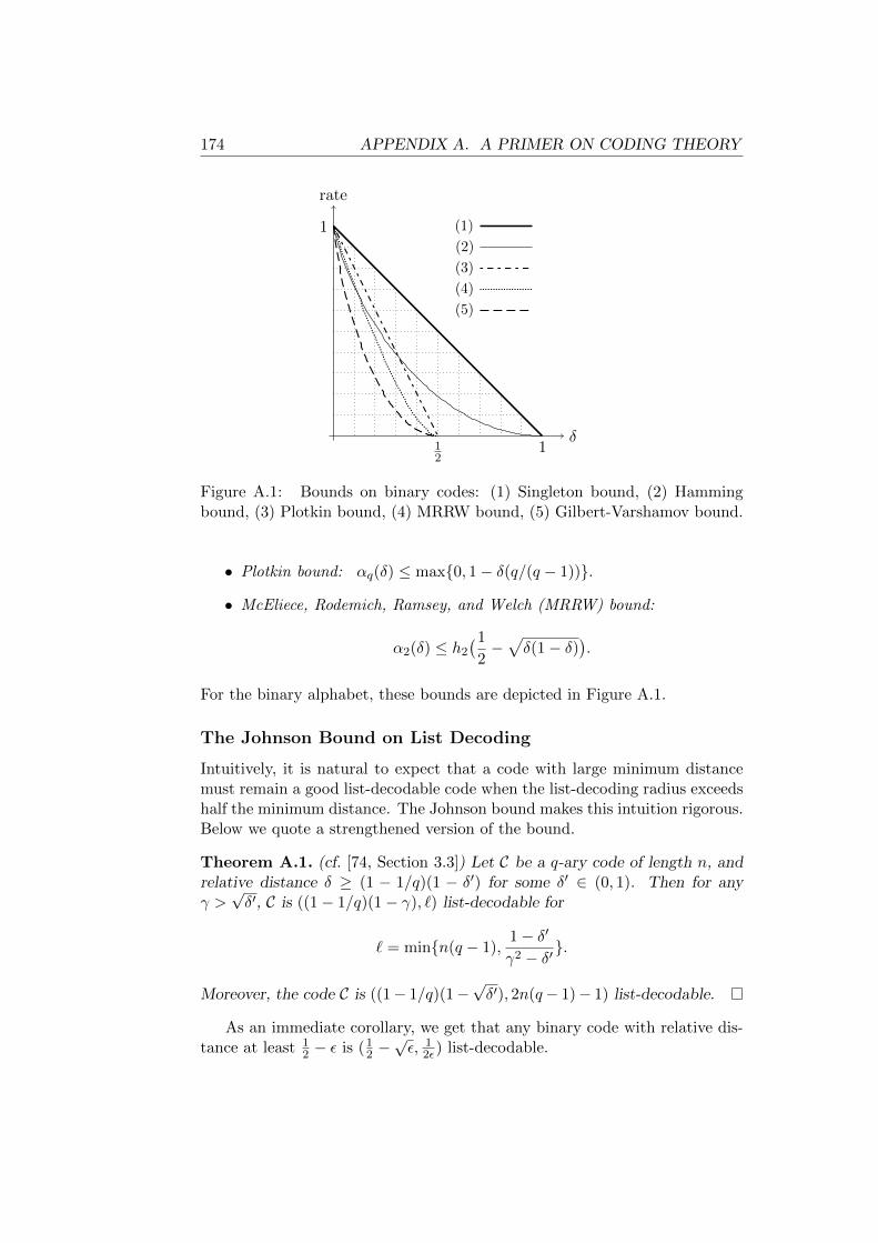
174 APPENDIX A. A PRIMER ON CODING THEORY
δ
rate
1
112
(1)
(2)
(3)
(4)
(5)
Figure A.1: Bounds on binary codes: (1) Singleton bound, (2) Hammingbound, (3) Plotkin bound, (4) MRRW bound, (5) Gilbert-Varshamov bound.
• Plotkin bound: αq(δ) ≤ max0, 1− δ(q/(q − 1)).
• McEliece, Rodemich, Ramsey, and Welch (MRRW) bound:
α2(δ) ≤ h2
(1
2−√δ(1− δ)
).
For the binary alphabet, these bounds are depicted in Figure A.1.
The Johnson Bound on List Decoding
Intuitively, it is natural to expect that a code with large minimum distancemust remain a good list-decodable code when the list-decoding radius exceedshalf the minimum distance. The Johnson bound makes this intuition rigorous.Below we quote a strengthened version of the bound.
Theorem A.1. (cf. [74, Section 3.3]) Let C be a q-ary code of length n, andrelative distance δ ≥ (1 − 1/q)(1 − δ′) for some δ′ ∈ (0, 1). Then for anyγ >√δ′, C is ((1− 1/q)(1− γ), `) list-decodable for
` = minn(q − 1),1− δ′γ2 − δ′ .
Moreover, the code C is ((1− 1/q)(1−√δ′), 2n(q− 1)− 1) list-decodable.
As an immediate corollary, we get that any binary code with relative dis-tance at least 1
2 − ε is (12 −√ε, 1
2ε) list-decodable.
A.3. REED-SOLOMON CODES 175
A.3 Reed-Solomon codes
Let p = (p1, . . . , pn) be a vector consisting of n distinct elements of Fq (assum-ing q ≥ n). The evaluation vector of a polynomial f : Fq → Fq with respectto p is the vector f(p) := (f(p1), . . . , f(pn)) ∈ Fnq .
A Reed-Solomon code of length n and dimension k over Fq is the set ofevaluation vectors of all polynomials of degree at most k − 1 over Fq withrespect to a particular choice of p. The dimension of this code is equal to k. Adirect corollary of Euclidean division algorithm states that, over any field, thenumber of zeros of any nonzero polynomial is less than or equal to its degree.Thus, we get that the minimum distance of a Reed-Solomon code is at leastn − k + 1, and because of the Singleton bound, is in fact equal to n − k + 1.Hence we see that a Reed-Solomon code is MDS. A generator matrix for aReed-Solomon code is given by the Vandermonde matrix
G :=
1 1 . . . 1p1 p2 . . . pnp2
1 p22 . . . p2
n...
.... . .
...
pk−11 pk−1
2 . . . pk−1n
.
A.4 The Hadamard Code
The Hadamard code of dimension n is a linear binary code of length 2n whosegenerator matrix can be obtained by arranging all binary sequences of lengthn as its columns. Each codeword of the Hadamard code can thus be seen asthe truth table of a linear form
`(x1, . . . , xn) =
n∑i=1
αixi
over the binary field. Therefore, each nonzero codeword must have weightexactly 2n−1, implying that the relative distance of the Hadamard code is 1
2 .
A.5 Concatenated Codes
Concatenation is a classical operation on codes that is mainly used for reducingthe alphabet size of a code. Suppose that C1 (called the outer code) is an(n1, k1, d1)Q-code and C2 (called the inner code) is a (n2, k2, d2)q-code, whereQ = qk2 . The concatenation of C1 and C2, that we denote by C1 C2 is an(n, k, d)q-code that can be conveniently defined by its encoder mapping asfollows.
Let x = (x1, . . . , xk1) ∈ [Q]k1 be the message given to the encoder, andC(x) = (c1, . . . , cn1) ∈ C1 be its encoding under C1. Each ci is thus an element
176 APPENDIX A. A PRIMER ON CODING THEORY
of [qk2 ] and can thus be seen as a q-ary string of length k2. Denote by c′i ∈ [q]n2
be the encoding of this string under C2. Then the encoding of x by theconcatenated code C1 C2 is the q-ary string of length n1n2
(c′′1, . . . , c′′n1
)
consisting of the string concatenation of symbol-wise encodings of C(x) usingC2.
Immediately from the above definition, one can see that n = n1n2, and k =k1k2. Moreover, it is straightforward to observe that the minimum distanceof the concatenated code satisfies d ≥ d1d2. When C1 and C2 are linear codes,the so is C1 C2.
As an example, let C1 be a Reed-Solomon code of length n1 := 2k2 anddimension k1 := 2δn1 over FQ, where Q := 2k2 . Thus the relative distance ofC1 equals 1− 2δ. As the inner code C2, take the Hadamard code of dimensionk2 and length Q. The concatenated code C := C1 C2 will thus have lengthn := Qn1 = 22k2 , dimension k := δk22k2+1, and relative distance at least12 − δ. Therefore, we obtain a binary [n, k, d] code where d ≥ (1
2 − δ)n, andn ≤ (k/δ)2. By the Johnson bound (Theorem A.1), this code must be (1
2−δ, `)list-decodable with list size at most 1/(2δ).
We remark that binary codes with relative minimum distance 12−δ and rate
Ω(δ3 log(1/δ)) (which only depends on the parameter δ) can be obtained byconcatenating Geometric Goppa codes on the Tsfasman-Vladut-Zink bound(see Section 4.3.2) with the Hadamard code. The Gilbert-Varshamov boundimplies that binary codes with relative distance 1
2 − δ and rate Ω(δ2) exist,and on the other hand, we know by the MRRW bound that O(δ2 log(1/δ)) isthe best rate one can hope for.
8 8Profondément calme (Dans une brume doucement sonore)
Claude Debussy (1862–1918): Preludes, Book I, No. X
(La cathedrale engloutie).

Bibliography
Number(s) following arrows (↑) indicate the page number(s) where the citation appears.
[1] M. Adler, E.D. Demaine, N.J.A. Harvey, and M. Patrascu, Lower boundsfor asymmetric communication channels and distributed source coding,Proceedings of the 17th symposium on discrete algorithms (SODA),2006, pp. 251–260. ↑24
[2] M. Adler and B. Maggs, Protocols for asymmetric communication chan-nels, Journal of Computer and System Sciences 63 (2001), no. 4, 573––596. ↑24
[3] M. Agrawal, N. Kayal, and N. Saxena, PRIMES is in P, Annals ofMathematics 160 (2004), no. 2, 781–793. ↑2, 10
[4] R. Ahlswede, N. Cai, S-Y. R. Li, and R. W. Yeung, Network informationflow, IEEE Transactions on Information Theory 46 (2000), no. 4, 1204–1216. ↑64
[5] N. Alon and J.H. Spencer, The probabilistic method, John Wiley andSons, 2000. ↑3, 11
[6] E. Ardestanizadeh, M. Cheraghchi, and A. Shokrollahi, Bit precisionanalysis for compressed sensing, Proceedings of IEEE international sym-posium on information theory (ISIT), 2009. ↑v
[7] E. Arıkan, Channel polarization: A method for constructing capacity-achieving codes for symmetric binary-input memoryless channels, IEEETransactions on Information Theory 55 (2009), no. 7, 3051–3073. ↑127
[8] S. Arora and B. Barak, Computational complexity: A modern approach,Cambridge University Press, 2009. ↑11
[9] B. Barak, A. Rao, R. Shaltiel, and A. Wigderson, 2-source dispersersfor sub-polynomial entropy and Ramsey graphs beating the Frankl-Wilsonconstruction, Proceedings of the 38th annual ACM symposium on theoryof computing (STOC), 2006, pp. 671–680. ↑4, 6
178
Bibliography 179
[10] A. Ben-Aroya and A. Ta-Shma, Constructing small-bias sets fromalgebraic-geometric codes, Proceedings of the 50th annual IEEE sym-posium on foundations of computer science (FOCS), 2009. ↑109
[11] C.H. Bennett, G. Brassard, and J-M. Robert, How to reduce your en-emy’s information, Proceedings of the 5th annual international cryptol-ogy conference (CRYPTO), 1985, pp. 468–476. ↑44
[12] E.R. Berlekamp, R. McEliece, and H.C.A van Tilborg, On the inherentintractability of certain coding problems, IEEE Transactions on Informa-tion Theory 24 (1978), 384–386. ↑172
[13] R.E. Blahut, Theory and practice of error control codes, Addison-Wesley,1983. ↑126
[14] A. Blass and Y. Gurevich, Pairwise testing, Bulletin of the EATCS 78(2002), 100–132. ↑77
[15] M. Blum and S. Micali, How to generate cryptographically strong se-quences of pseudorandom bits, SIAM Journal on Computing 13 (1984),no. 4, 850–864. ↑154
[16] J. Bourgain, On the construction of affine extractors, Geometric andFunctional Analysis 17 (2007), no. 1, 33–57. ↑49, 62
[17] , Personal Communication, 2008. ↑62
[18] W.J. Bruno, E. Knill, D.J. Balding, D.C. Bruce, N.A. Doggett, W.W.Sawhill, R.L. Stallings, C.C. Whittaker, and D.C. Torney, Efficient pool-ing designs for library screening, Genomics 26 (1995), no. 1, 21–30. ↑77
[19] H. Buhrman, P.B. Miltersen, J. Radhakrishnan, and S. Venkatesh, Arebitvectors optimal?, SIAM Journal on Computing 31 (2002), no. 6, 1723–1744. ↑102
[20] J. Buresh-Oppenheim, V. Kabanets, and R. Santhanam, Uniform hard-ness amplification in NP via monotone codes, 2006. ECCC TechnicalReport TR06-154. ↑88
[21] N. Cai and R. W. Yeung, Secure network coding, Proceedings of IEEEinternational symposium on information theory (ISIT), 2002. ↑65
[22] R. Canetti, Y. Dodis, S. Halevi, E. Kushilevitz, and A. Sahai, Exposure-resilient functions and all-or-nothing transforms, Proceedings of the 19thannual international cryptology conference (CRYPTO), 1999, pp. 503–518. ↑44, 46, 47, 68
[23] M. Capalbo, O. Reingold, S. Vadhan, and A. Wigderson, Randomnessconductors and constant-degree expansion beyond the degree/2 barrier,Proceedings of the 34th annual ACM symposium on theory of computing(STOC), 2002, pp. 659–668. ↑25, 98, 99, 120
[24] H. Chang, H-B. Chen, H-L. Fu, and C-H. Shi, Reconstruction of hiddengraphs and threshold group testing, Journal of Combinatorial Optimiza-tion (2010). ↑103
180 Bibliography
[25] D. X. Charles, K. E. Lauter, and E. Z. Goren, Cryptographic hash func-tions from expander graphs, Journal of Cryptology (2007). ↑56
[26] H-B. Chen, D-Z. Du, and F-K. Hwang, An unexpected meeting of fourseemingly unrelated problems: graph testing, DNA complex screening,superimposed codes and secure key distribution, Journal of CombinatorialOptimization 14 (2007), no. 2-3, 121–129. ↑77, 104, 106, 123
[27] H-B. Chen and H-L. Fu, Nonadaptive algorithms for threshold grouptesting, Discrete Applied Mathematics 157 (2009), 1581–1585. ↑103, 105,106, 167
[28] H-B. Chen, H-L. Fu, and F-K. Hwang, An upper bound of the number oftests in pooling designs for the error-tolerant complex model, Optimiza-tion Letters 2 (2008), no. 3, 425–431. ↑106, 123
[29] Y. Cheng and D-Z. Du, New constructions of one- and two-stage poolingdesigns, Journal of Computational Biology 15 (2008), no. 2, 195–205.↑115
[30] M. Cheraghchi, Noise-resilient group testing: Limitations and construc-tions, Proceedings of the 17th international symposium on fundamentalsof computation theory (FCT), 2009, pp. 62–73. ↑vi
[31] , Improved constructions for non-adaptive threshold group test-ing, Proceedings of the 37th international colloquium on automata, lan-guages and programming (ICALP), 2010. arXiv: cs.DM/1002.2244. ↑vi
[32] M. Cheraghchi, F. Didier, and A. Shokrollahi, Invertible extractors andwiretap protocols, Proceedings of IEEE international symposium on in-formation theory (ISIT), 2009. ↑iv
[33] M. Cheraghchi, A. Hormati A. Karbasi, and M. Vetterli, Compressedsensing with probabilistic measurements: A group testing solution, Pro-ceedings of the annual Allerton conference on communication, control,and computing, 2009. ↑v
[34] M. Cheraghchi, A. Karbasi, S. Mohajer, and V. Saligrama, Graph-constrained group testing, Proceedings of IEEE international symposiumon information theory (ISIT), 2010. ↑v
[35] B. Chor and O. Goldreich, Unbiased bits from sources of weak random-ness and probabilistic communication complexity, SIAM Journal of Com-puting 17 (1988), no. 2, 230–261. ↑4, 6
[36] B. Chor, O. Goldreich, J. Hastad, J. Friedmann, S. Rudich, and R.Smolensky, The bit extraction problem or t-resilient functions, Proceed-ings of the 26th annual IEEE symposium on foundations of computerscience (FOCS), 1985, pp. 396–407. ↑44, 45
[37] R. Clifford, K. Efremenko, E. Porat, and A. Rothschild, k-mismatch withdon’t cares, Proceedings of the 15th european symposium on algorithm(ESA), 2007, pp. 151–162. ↑77
Bibliography 181
[38] G. Cormode and S. Muthukrishnan, What’s hot and what’s not: track-ing most frequent items dynamically, ACM Transactions on DatabaseSystems 30 (2005), no. 1, 249–278. ↑77
[39] , Combinatorial algorithms for compressed sensing, Proceedingsof information sciences and systems, 2006, pp. 198–201. ↑77
[40] T.M. Cover and J.A. Thomas, Elements of information theory, Second,John Wiley and Sons, 2006. ↑17, 24, 131, 132
[41] I. Csiszar and J. Korner, Broadcast channels with confidential messages,IEEE Transactions on Information Theory 24 (1978), no. 3, 339–348.↑64
[42] P. Damaschke, Threshold group testing, General theory of informationtransfer and combinatorics, 2006, pp. 707–718. ↑103
[43] A. De Bonis, L. Gasieniec, and U. Vaccaro, Optimal two-stage algorithmsfor group testing problems, SIAM Journal on Computing 34 (2005),no. 5, 1253–1270. ↑123
[44] M. DeVos and A. Gabizon, Simple affine extractors using dimensionexpansion, Proceedings of the 25th IEEE conference on computationalcomplexity (CCC), 2010. ↑49
[45] Y. Dodis, Exposure-resilient cryptography, Ph.D. Thesis, 2000. ↑7, 44
[46] , On extractors, error-correction and hiding all partial informa-tion, Proceedings of the IEEE information theory workshop (ITW),2005. ↑53
[47] Y. Dodis, A. Sahai, and A. Smith, On perfect and adaptive secu-rity in exposure-resilient cryptography, Proceedings of Eurocrypt, 2001,pp. 301–324. ↑43, 45, 54
[48] Y. Dodis and A. Smith, Entropic security and the encryption of high-entropy messages, Proceedings of the theory of cryptography conference(TCC), 2005, pp. 556–577. ↑53
[49] R. Dorfman, The detection of defective members of large populations,Annals of Mathematical Statistics 14 (1943), 436–440. ↑76
[50] D-Z. Du and F. Hwang, Combinatorial group testing and its applications,Second, World Scientific, 2000. ↑11, 77, 104, 123
[51] D-Z. Du and F-K. Hwang, Pooling designs and nonadaptive group test-ing, World Scientific, 2006. ↑11, 77, 104
[52] I. Dumer, D. Micciancio, and M. Sudan, Hardness of approximating theminimum distance of a linear code, IEEE Transactions on InformationTheory 49 (2003), no. 1, 22–37. ↑161
[53] A. D’yachkov, P. Vilenkin, A. Macula, and D. Torney, Families of finitesets in which no intersection of ` sets is covered by the union of s others,Journal of Combinatorial Theory, Series A 99 (2002), 195–218. ↑106, 123
182 Bibliography
[54] A.G. D’yachkov and V.V. Rykov, Bounds of the length of disjunct codes,Problems of Control and Information Theory 11 (1982), 7–13. ↑83, 102
[55] S. Y. El Rouayheb and E. Soljanin, On wiretap networks II, Proceedingsof IEEE international symposium on information theory (ISIT), 2007,pp. 24–29. ↑65
[56] D. Eppstein, M.T. Goodrich, and D.S. Hirschberg, Improved combinato-rial group testing algorithms for real-world problem sizes, SIAM Journalon Computing 36 (2007), no. 5, 1360–1375. ↑123
[57] P. Erdos, Some remarks on the theory of graphs, Bulletin of the AmericanMathematical Society 53 (1947), 292–294. ↑4
[58] M. Farach, S. Kannan, E. Knill, and S. Muthukrishnan, Group testingproblems with sequences in experimental molecular biology, Proceedingsof compression and complexity of sequences, 1997, pp. 357–367. ↑77
[59] J. Feldman, T. Malkin, R. Servedio, and C. Stein, On the capacity ofsecure network coding, Proceedings of the annual Allerton conference oncommunication, control, and computing, 2004. ↑65
[60] G.D. Forney, Concatenated codes, MIT Press, 1966. ↑127, 142, 143
[61] K. Friedl and S-C. Tsai, Two results on the bit extraction problem, Dis-crete Applied Mathematics and Combinatorial Operations Research andComputer Science 99 (2000). ↑44
[62] J. Friedmann, On the bit extraction problem, Proceedings of the 33rdannual IEEE symposium on foundations of computer science (FOCS),1992, pp. 314–319. ↑44
[63] Z. Furedi, On r-cover-free families, Journal of Combinatorial Theory,Series A 73 (1996), 172–173. ↑83
[64] E.M. Gabidulin, Theory of codes with maximum rank distance (trans-lation), Problems of Information Transmission 21 (1985), no. 1, 1–12.↑51
[65] A. Gabizon and R. Raz, Deterministic extractors for affine sources overlarge fields, Proceedings of the 46th annual IEEE symposium on foun-dations of computer science (FOCS), 2005, pp. 407–418. ↑49, 59, 60,62
[66] H. Gao, F.K. Hwang, M.T. Thai, W. Wu, and T. Znati, Construction ofd(H)-disjunct matrix for group testing in hypergraphs, Journal of Com-binatorial Optimization 12 (2006), 297–301. ↑104, 106
[67] A. Garcia and H. Stichtenoth, A tower of Artin-Schreier extensions offunction fields attaining the Drinfeld-Vladut bound, Invent. Math. 121(1995), 211–222. ↑108, 151
[68] E.N. Gilbert, A comparison of signaling alphabets, Bell System TechnicalJournal 31 (1952), 504–522. ↑47, 150, 159
Bibliography 183
[69] M.X. Goemans and D.P. Williamson, Improved approximation algo-rithms for maximum cut and satisfiability problems using semidefiniteprogramming, Journal of the ACM 42 (1995), 1115–1145. ↑2
[70] O. Goldreich, Computational complexity: A conceptual perspective, Cam-bridge University Press, 2008. ↑9, 11
[71] O. Goldreich and D. Zuckerman, Another proof that BPP ⊆ PH(and more), 1997. ECCC Technical Report TR97-045 (available onlineat http://eccc.hpi-web.de/eccc-reports/1997/TR97-045/index.
html). ↑7[72] V.D. Goppa, Codes on algebraic curves, Soviet Mathematics Doklady
24 (1981), 170–172. ↑47, 151
[73] R. Gradwohl, S. Vadhan, and D. Zuckerman, Random selection withan adversarial majority, Proceedings of the 26th annual internationalcryptology conference (CRYPTO), 2006. ↑7
[74] V. Guruswami, List decoding of error-correcting codes, Ph.D. Thesis,2001. ↑11, 101, 174
[75] V. Guruswami and P. Gopalan, Hardness amplification within NPagainst deterministic algorithms, Proceedings of the 23rd IEEE confer-ence on computational complexity (CCC), 2008, pp. 19–30. ↑88
[76] V. Guruswami and P. Indyk, Linear-time encodable/decodable codes withnear-optimal rate, IEEE Transactions on Information Theory 51 (2005),no. 10, 3393–3400. ↑142
[77] V. Guruswami and A. Rudra, Concatenated codes can achieve list decod-ing capacity, Proceedings of the 19th symposium on discrete algorithms(SODA), 2008. ↑101
[78] V. Guruswami, C. Umans, and S. Vadhan, Unbalanced expanders andrandomness extractors from Parvaresh-Vardy codes, Journal of the ACM56 (2009), no. 4. ↑35, 37, 38, 39, 91, 93, 101, 167
[79] J. Hastad, Some optimal inapproximability results, Journal of theACM 48 (2001), no. 4, 798–859. Preliminary version in Proceedings ofSTOC’97. ↑2
[80] J. Hastad, R. Impagliazzo, L. Levin, and M. Luby, A pseudorandomgenerator from any one-way function, SIAM Journal on Computing 28(1999), no. 4, 1364–1396. ↑154
[81] E-S. Hong and R.E. Ladner, Group testing for image compression, Datacompression conference, 2000, pp. 3–12. ↑77
[82] S. Hoory, N. Linial, and A. Wigderson, Expander graphs and their ap-plications, Bulletin of the American Mathematical Society 43 (2006),no. 4, 439–561. ↑11, 55
[83] J. Hopcroft, W. Paul, and L. Valiant, On time versus space, Journal ofthe ACM 24 (1977), 332–337. ↑157
184 Bibliography
[84] R. Impagliazzo, L. Levin, and M. Luby, Pseudorandom generation fromone-way functions, Proceedings of the 21st annual ACM symposium ontheory of computing (STOC), 1989, pp. 12–24. ↑26
[85] R. Impagliazzo and A. Wigderson, P = BPP unless E has sub-exponentialcircuits: derandomizing the XOR lemma, Proceedings of the 29th annualACM symposium on theory of computing (STOC), 1997, pp. 220–229.↑157, 161
[86] P. Indyk, Explicit construction of compressed sensing of sparse signals,Proceedings of the 19th symposium on discrete algorithms (SODA),2008. ↑7
[87] J. Justesen, A class of constructive asymptotically good algebraic codes,IEEE Transactions on Information Theory 18 (1972), 652–656. ↑127,142
[88] J. Kamp and D. Zuckerman, Deterministic extractors for bit-fixingsources and exposure-resilient cryptography, SIAM Journal on Comput-ing 36 (2006), 1231–1247. ↑55, 56
[89] W.H. Kautz and R.C. Singleton, Nonrandom binary superimposed codes,IEEE Transactions on Information Theory 10 (1964), 363–377. ↑100,102, 106, 107, 108
[90] S. Khot, G. Kindler, E. Mossel, and R. O’Donnell, Optimal inapproxima-bility results for MAX-CUT and other two-variable CSPs?, Proceedingsof the 45th annual IEEE symposium on foundations of computer science(FOCS), 2004, pp. 146–154. ↑2
[91] H.K. Kim and V. Lebedev, On optimal superimposed codes, Journal ofCombinatorial Designs 12 (2004), 79–91. ↑106, 123
[92] A. Klivans and D. van Melkebeek, Graph nonisomorphism has sub-exponential size proofs unless the polynomial-time hierarchy collapses,SIAM Journal on Computing 31 (2002), no. 5, 1501–1526. ↑161
[93] E. Knill, Lower bounds for identifying subset members with subsetqueries, Proceedings of the 6th symposium on discrete algorithms(SODA), 1995, pp. 369–377. ↑88
[94] R. Kotter and M. Medard, An algebraic approach to network coding,IEEE/ACM Transactions on Networking 11 (2003), no. 5, 782–795. ↑64
[95] F. R. Kschischang and D. Silva, Security for wiretap networks via rank-metric codes, 2007. Unpublished manuscript (arXiv: cs.IT/0801.0061).↑66, 67
[96] K. Kurosawa, T. Johansson, and D. Stinson, Almost k-wise independentsample spaces and their cryptologic applications, Journal of Cryptology14 (2001), no. 4, 231–253. ↑44, 47
[97] S-Y. R. Li, R. W. Yeung, and N. Cai, Linear network coding, IEEETransactions on Information Theory 49 (2003), no. 2, 371–381. ↑64
Bibliography 185
[98] J. H. van Lint, Introduction to coding theory, Third, Graduate Texts inMathematics, vol. 86, Springer Verlag, 1998. ↑11, 170
[99] L. Lovasz, Random walks on graphs: A survey, Combinatorics, PaulErdos is Eighty, Vol. 2 (ed. D. Miklos, V. T. Sos, T. Szonyi), JanosBolyai Mathematical Society, Budapest (1996), 353–398. ↑56
[100] A. Lubotzky, R. Phillips, and P. Sarnak, Ramanujan graphs, Combina-torica 8 (1988), 261–277. ↑59
[101] M. Luby, LT-codes, Proceedings of the 43rd annual IEEE symposiumon foundations of computer science (FOCS), 2002, pp. 271–280. ↑63
[102] A.J. Macula, Probabilistic nonadaptive group testing in the presence oferrors and DNA library screening, Annals of Combinatorics 3 (1999),no. 1, 61–69. ↑77
[103] F.J. MacWilliams and N.J. Sloane, The theory of error-correcting codes,North Holand, 1977. ↑11, 110, 170
[104] S. Mahajan and H. Ramesh, Derandomizing semidefinite programmingbased approximation algorithms, Proceedings of the 36th annual IEEEsymposium on foundations of computer science (FOCS), 1995, pp. 162–169. ↑2
[105] Yu.I. Manin, What is the maximum number of points on a curve overF2?, Journal of the Faculty of Science, University of Tokyo 28 (1981),715–720. ↑150
[106] J.L. Massey, Threshold decoding, MIT Press, Cambridge, Massachusetts,USA, 1963. ↑160
[107] G.L. Miller, Riemann’s hypothesis and tests for primality, Journal ofComputer and System Sciences 13 (1976), no. 3, 300–317. ↑2
[108] P.B. Miltersen, Derandomizing complexity classes, Book chapter inHandbook of Randomized Computing, Kluwer Academic Publishers(2001). ↑158
[109] M. Mitzenmacher and E. Upfal, Probability and computing, CambridgeUniversity Press, 2005. ↑11, 55
[110] M. Morgenstern, Existence and explicit constructions of q + 1 regularramanujan graphs for every prime power q, Journal of CombinatorialTheory, Series B 62 (1994), 44–62. ↑59
[111] E. Mossel and C. Umans, On the complexity of approximating the VCdimension, Proceedings of the 16th IEEE conference on computationalcomplexity (CCC), 2001, pp. 220–225. ↑7
[112] R. Motwani and P. Raghavan, Randomized algorithms, Cambridge Uni-versity Press, 1995. ↑11, 55
186 Bibliography
[113] H-Q. Ngo and D-Z. Du, A survey on combinatorial group testing algo-rithms with applications to DNA library screening, DIMACS Series onDiscrete Math. and Theoretical Computer Science 55 (2000), 171–182.↑77
[114] A. Nilli, On the second eigenvalue of a graph, Discrete Mathematics 91(1991), 207–210. ↑58
[115] N. Nisan and A. Wigderson, Hardness vs. randomness, Journal of Com-puter and Systems Sciences 49 (1994), no. 2, 149–167. ↑10, 151, 154,155, 161
[116] L. H. Ozarow and A. D. Wyner, Wire-tap channel II, AT&T Bell Lab-oratories Technical Journal 63 (1984), 2135–2157. ↑41, 46, 55, 65
[117] C.H. Papadimitriou, Computational complexity, Addison-Wesley, 1994.↑152
[118] F. Parvaresh and A. Vardy, Correcting errors beyond the Guruswami-Sudan radius in polynomial time, Proceedings of the 46th annual IEEEsymposium on foundations of computer science (FOCS), 2005, pp. 285–294. ↑35, 100
[119] A. K. Pizer, Ramanujan graphs and Hecke operators, Bulletin of theAmerican Mathematical Society 23 (1990), no. 1, 127–137. ↑59
[120] E. Porat and A. Rothschild, Explicit non-adaptive combinatorial grouptesting schemes, Proceedings of the 35th international colloquium onautomata, languages and programming (ICALP), 2008, pp. 748–759.↑106, 110, 122
[121] M. Rabin, Probabilistic algorithm for testing primality, Journal of Num-ber Theory 12 (1980), no. 1, 128–138. ↑2
[122] J. Radhakrishan and A. Ta-Shma, Tight bounds for depth-two supercon-centrators, Proceedings of the 38th annual IEEE symposium on founda-tions of computer science (FOCS), 1997, pp. 585–594. ↑25, 120
[123] R. Raz, O. Reingold, and S. Vadhan, Extracting all the randomnessand reducing the error in Trevisan’s extractor, Journal of Computer andSystem Sciences 65 (2002), no. 1, 97–128. ↑34, 60, 99
[124] R. Raz and A. Yehudayoff, Multilinear formulas, maximal-partition dis-crepancy and mixed-sources extractors, Proceedings of the 49th annualIEEE symposium on foundations of computer science (FOCS), 2008. ↑6
[125] T. Richardson and R. Urbanke, Modern coding theory, Cambridge Uni-versity Press, 2008. ↑126
[126] R. Rivest, All-or-nothing encryption and the package transform, Pro-ceedings of the international workshop on fast software encryption, 1997,pp. 210–218. ↑44, 45
[127] R.M. Roth, Introduction to coding theory, Cambridge University Press,2006. ↑11, 127, 170
Bibliography 187
[128] A. Russell and D. Zuckerman, Perfect information leader election inlog∗ n + o(1) rounds, Journal of Computer and Systems Sciences 63(2001), 612–626. ↑7
[129] Ruszinko, On the upper bound of the size of the r-cover-free families,Journal of Combinatorial Theory, Series A 66 (1994), 302–310. ↑83
[130] A. Schliep, D. Torney, and S. Rahmann, Group testing with DNA chips:Generating designs and decoding experiments, Proceedings of computa-tional systems bioinformatics, 2003. ↑77
[131] J. T. Schwartz, Fast probabilistic algorithms for verification of polyno-mial identities, Journal of the ACM 27 (1980), no. 4, 701–717. ↑3
[132] R. Shaltiel, How to get more mileage from randomness extractors, Pro-ceedings of the 21st annual conference on computational complexity,2006, pp. 46–60. ↑59, 60, 165
[133] , Weak derandomization of weak algorithms: explicit versions ofyao’s lemma, Proceedings of the 24th annual conference on computa-tional complexity, 2009. ↑165
[134] R. Shaltiel and C. Umans, Simple extractors for all min-entropies anda new pseudorandom generator, Journal of the ACM 52 (2005), no. 2,172–216. ↑60, 99
[135] A. Shamir, On the generation of cryptographically strong pseudorandomsequences, ACM Transactions on Computer Systems 1 (1983), no. 1,38–44. ↑154
[136] C.E. Shannon, A mathematical theory of communication, The Bell Sys-tem Technical Journal 27 (1948), 379–423 and 623–656. ↑5, 126, 131
[137] A. Shokrollahi, Raptor codes, IEEE Transactions on Information Theory52 (2006), 2551–2567. ↑63, 126
[138] V. Shoup, New algorithms for finding irreducible polynomials over finitefields, Mathematics of Computation 54 (1990), 435–447. ↑38
[139] M. Sipser, Introduction to the theory of computation, Second, CourseTechnology, 2005. ↑152
[140] R.M. Solovay and V. Strassen, A fast Monte-Carlo test for primality,SIAM Journal on Computing 6 (1977), no. 1, 84–85. ↑2
[141] D. Spielman, Linear-time encodable and decodable error-correcting codes,IEEE Transactions on Information Theory 42 (1996), 1723–1731. ↑142
[142] H. Stichtenoth, Algebraic function fields and codes, Springer, 1993. ↑109
[143] D. Stinson, Resilient functions and large set of orthogonal arrays, Con-gressus Numerantium 92 (1993), 105–110. ↑44
[144] D.R. Stinson and R. Wei, Generalized cover-free families, Discrete Math-ematics 279 (2004), 463–477. ↑106, 123
188 Bibliography
[145] D.R. Stinson, R. Wei, and L. Zhu, Some new bounds for cover-free fam-ilies, Journal of Combinatorial Theory, Series A 90 (2000), 224–234.↑106, 123
[146] M. Sudan, L. Trevisan, and S. Vadhan, Pseudorandom generators with-out the XOR lemma, Journal of Computer and Systems Sciences 62(2001), no. 2, 236–266. ↑157
[147] A. Ta-Shma, Storing information with extractors, Information Process-ing Letters 83 (2002), no. 5, 267–274. ↑7, 102
[148] A. Ta-Shma, C. Umans, and D. Zuckerman, Lossless condensers, unbal-anced expanders, and extractors, Proceedings of the 33rd annual ACMsymposium on theory of computing (STOC), 2001, pp. 143–152. ↑100
[149] A. Ta-Shma and D. Zuckerman, Extractor codes, IEEE Transactions onInformation Theory 50 (2004), no. 12, 3015–3025. ↑7, 91, 93, 99, 101
[150] A. Ta-Shma, D. Zuckerman, and S. Safra, Extractors from Reed-Mullercodes, Journal of Computer and System Sciences 72 (2006), 786–812.↑60
[151] J-P. Tillich and G. Zemor, Collisions for the lps expander graph hashfunction, Proceedings of Eurocrypt, 2008, pp. 254–269. ↑56
[152] L. Trevisan, Extractors and pseudorandom generators, Journal of theACM 48 (2001), no. 4, 860–879. ↑28, 32, 34, 60, 99
[153] L. Trevisan and S. Vadhan, Extracting randomness from samplable dis-tributions, Proceedings of the 41st annual IEEE symposium on founda-tions of computer science (FOCS), 2000, pp. 32–42. ↑19, 165
[154] M.A. Tsfasman, S.G. Vladut, and Th. Zink, Modular curves, Shimuracurves, and Goppa codes better than the Varshamov-Gilbert bound,Mathematische Nachrichten 109 (1982), 21–28. ↑47, 108, 151, 168
[155] S. Vadhan, The unified theory of pseudorandomness, Proceedings of theinternational congress of mathematicians, 2010. ↑91
[156] A. Vardy, The intractability of computing the minimum distance of acode, IEEE Transactions on Information Theory 43 (1997), no. 6, 1757–1766. ↑161
[157] R. R. Varshamov, Estimate of the number of signals in error correctingcodes, Doklady Akademii Nauk SSSR 117 (1957), 739–741. ↑47, 150,159, 160
[158] U.V. Vazirani, Towards a strong communication complexity theoryor generating quasi-random sequences from two communicating semi-random sources, Combinatorica 7 (1987), no. 4, 375–392. ↑44
[159] J. von Neumann, Various techniques used in connection with randomdigits, Applied Math Series 12 (1951), 36–38. ↑12
Bibliography 189
[160] J. Watkinson, M. Adler, and F.E. Fich, New protocols for asymmet-ric communication channels, Proceedings of international colloquiumon structural information and communication complexity (SIROCCO),2001. ↑24
[161] A. Wigderson and D. Zuckerman, Expanders that beat the eigenvaluebound: explicit construction and applications, Combinatorica 19 (1999),no. 1, 125–138. ↑6
[162] J. Wolf, Born-again group testing: multiaccess communications, IEEETransactions on Information Theory 31 (1985), 185–191. ↑77
[163] W. Wu, Y. Huang, X. Huang, and Y. Li, On error-tolerant DNA screen-ing, Discrete Applied Mathematics 154 (2006), no. 12, 1753–1758. ↑77
[164] W. Wu, Y. Li, C.H. Huang, and D.Z. Du, Molecular biology and poolingdesign, Data Mining in Biomedicine 7 (2008), 133–139. ↑77
[165] A. D. Wyner, The wire-tap channel, The Bell System Technical Journal54 (1975), 1355–1387. ↑40
[166] A. Yao, Theory and applications of trapdoor functions, Proceedings ofthe 23rd annual IEEE symposium on foundations of computer science(FOCS), 1982, pp. 80–91. ↑154
[167] A. Yehudayoff, Affine extractors over prime fields, 2009. Unpublishedmanuscript. ↑49, 62
[168] R. W. Yeung, S-Y. R. Li, N. Cai, and Z. Zhang, Network coding theory,Foundations and Trends in Communications and Information Theory,2005. ↑64
[169] R. E. Zippel, Probabilistic algorithms for sparse polynomials, SpringerLecture Notes in Computer Science (EUROSCAM’79) 72 (1979), 216–226. ↑3
[170] D. Zuckerman, On unapproximable versions of NP-complete problems,SIAM Journal of Computing 25 (1996), 1293–1304. ↑7
[171] , Randomness-optimal oblivious sampling, Random Structuresand Algorithms 11 (1997), no. 4, 345–367. ↑7
[172] , Linear degree extractors and the inapproximability of MaxClique and Chromatic Number, Theory of Computing 3 (2007), no. 6,103–128. ↑56
Index
agreement list, 94all-or-nothing transform (AONT)
average case, 47all-or-nothing transform (AONT),
47asymmetric communication, 24asymptotically perfect privacy, 43
channel, 132q-ary symmetric, 133binary symmetric (BSC), 133binary erasure (BEC), 133memoryless, 132symmetric, 132
code, 174asymptotically good, 175binary, 174capacity achieving, 136concatenation, 179dual, 175ensemble, 136error exponent, 136explicit, 175family, 136Gabidulin, 54Hadamard, 179length, 174linear, 175
dimension, 175generator matrix, 175parity check matrix, 175
list decodable, 176
MDS, 177minimum distance, 174MRD, 54rank-metric, 53rate, 174Reed-Solomon, 179size, 174
codeword, 174codeword graph, 94condenser, 21
lossless, 22consistent labeling, 58
direct channel, 43disjunct
(d, e)-disjunct, 82(d, e;u)-disjunct, 114d-disjunct, 82lower bound, 85strongly disjunct, 106upper bound, 84
disjunctive query, 79distance decoder, 83distribution
flat, 17
entropy function, 177equivocation, 43exposure-resilient function (ERF),
46extractor, 20
affine, 50
190
INDEX 191
explicit, 20Kamp and Zuckerman’s, 58strong, 20symbol-fixing, 50
false negative, 89false positive, 89
Gilbert-Varshamov bound, 177group testing
classical formulation, 79two-stage schemes, 90
group testinghypergraph learning, 106threshold model, 105threshold model
gap, 105
Hamming distance, 174Hamming weight, 80, 174Hermitian codes, 111hypergraph, 106
induced code, 94invertible extractor, 55
Justesen’s concatenation, 147
Kautz-Singleton construction, 108
Leftover Hash Lemma, 27
measurement matrix, 81mixture, 94
notation[n] := 1, . . . , n, 26UΩ,Un, 14M [x], 81X (T ),PrX [T ], 13X (x),PrX (x), 13Fq := GF(q), 19x>, 51M1 M2, 116(e0, e1)-close, 80‖X − Y‖p, 14
M, S for matrix M80M [i, j] for matrix M , 80supp(x), 80wgt(x), 80x(i) for vector x, 80
Ozarow-Wyner’s protocol, 49
perfect privacy, 43probability distribution
ε-close, 14distance, 14support of, 13
quasipolynomial, 132
rank metric, 53regular matrix, 114resilient function (RF), 46resilient matrix, 88
Singleton bound, 177source
affine, 50Fq-restricted, 53
bit-fixing, 49spectral gap, 58sprase vector, 79statistical distance, 14strong secrecy, 43sublinear time reconstruction, 101support, 80syndrome decoding, 176
TVZ bound, 110
universal hash family, 26
weak secrecy, 43wiretap protocol
error, 45resilience, 45
wiretap channel, 43wiretap protocol, 44
leakage, 45rate, 45
wiretap II problem, 43