1

Information Theoretic Measures for Power Analysis1

Diana Marculescu, Radu Marculescu, Massoud Pedram

Department of Electrical Engineering - Systems

University of Southern California, Los Angeles, CA 90089

Abstract - This paper considers the problem of estimating the power consumption at logic and register

transfer levels of design from an information theoretical point of view. In particular, it is demonstrated that the

average switching activity in the circuit can be calculated using either entropy or informational energy averages.

For control circuits and random logic, the output entropy (informational energy) per bit is calculated as a

function of the input entropy (informational energy) per bit and an implementation dependent information scaling

factor. For data-path circuits, the output entropy (informational energy) is calculated from the input entropy

(informational energy) using a compositional technique which has linear complexity in terms of the circuit size.

Finally, from these input and output values, the entropy (informational energy) per circuit line is calculated and

used as an estimate for the average switching activity. The proposed switching activity estimation technique does

not require simulation and is thus extremely fast, yet produces sufficiently accurate estimates.

I. INTRODUCTION

Modern design tools have changed the entire design process of digital systems. As a result, most of the

systems are conceived and designed today at the behavioral/logic level, with little or no knowledge of the final

gate level implementation and the layout style. In particular, designers are becoming more and more interested

in register-transfer level (RTL) modules (adders, multipliers, registers, multiplexers) and strategies to put them

together in order to build complex digital systems. Power minimization in digital systems is not an exception to

this trend. Having as soon as possible in the design cycle an estimate of power consumption, can save

significant redesign efforts or even completely change the entire design architecture.

A. Basic Issues and Prior Work

Gate-level power estimation techniques can be divided into two general categories: simulative and non-

simulative [1][2]. Simulative techniques have their roots in direct simulation and sampling techniques [3]-[5].

The main advantages of these techniques are that existing simulators can be used for estimation purposes and

1This research was supported in part by Advanced Research Project Agency under Contract F33615-95-C-1627 andby Semiconductor Research Corporation under contract 94-DJ-559.

2

issues such as hazard generation and propagation, reconvergent fanout induced correlations are automatically

taken into consideration. The disadvantage is their strong input pattern dependence and long running times (in

sampling techniques this is needed for achieving high levels of accuracy). Non-simulative techniques are based

on probabilistic or stochastic techniques [6]-[9]. Their main advantages are higher speed and lower dependence

on the input patterns. Generally speaking, however, they tend to be less accurate due to the simplified models

used and the approximations made in order to achieve higher efficiency.

Higher levels of abstraction have also been considered, but here many problems are still pending a

satisfactory solution. At this level, consistency is more important than accuracy, that is, relative (as opposed to

absolute) evaluation of different designs is often sufficient. Most of the high level prediction tools combine

deterministic analysis with profiling and simulation in order to address data dependencies. Important statistics

include the number of instructions of a given type, the number of bus, register and memory accesses, and the

number of I/O operations executed within a given period [10][11]. Analytic modeling efforts have been

described in [12] where a parametric power model was developed for macromodules. However, the trade-off

between flexibility and accuracy is still a challenging task as major difficulties persist due to the lack of precise

information and the conceptual complexity which characterizes this level of design abstraction.

Power dissipation in CMOS circuits comes from three sources: leakage currents which include the reverse-

biased p-n junction and subthreshold currents, short-circuit currents which flow due to the DC path between the

supply rails during output transitions and capacitive switching currents which are responsible for charging and

discharging of capacitive loads during logic transitions. In well-designed circuits with relatively high threshold

voltages, the first two sources are small compared to the last one. Therefore, to estimate the total power

consumption of a module (in a gate level implementation), we may only account for the capacitive switching

currents, yet achieve sufficient levels of accuracy [13]:

(1)

where fclk is the clock frequency, VDD is the supply voltage, Cn and swn are the capacitive load and the average

switching activity of gate n, respectively (the summation is performed over all gates in the circuit). As we can

see, in this formulation the average switching activity per node is a key factor, and therefore its correct

calculation is essential for accurate power estimation. Note that for the same implementation of a module,

different input sequences may give rise to different switching activities at the circuit inputs and at the outputs of

internal gates and consequently completely different power values.

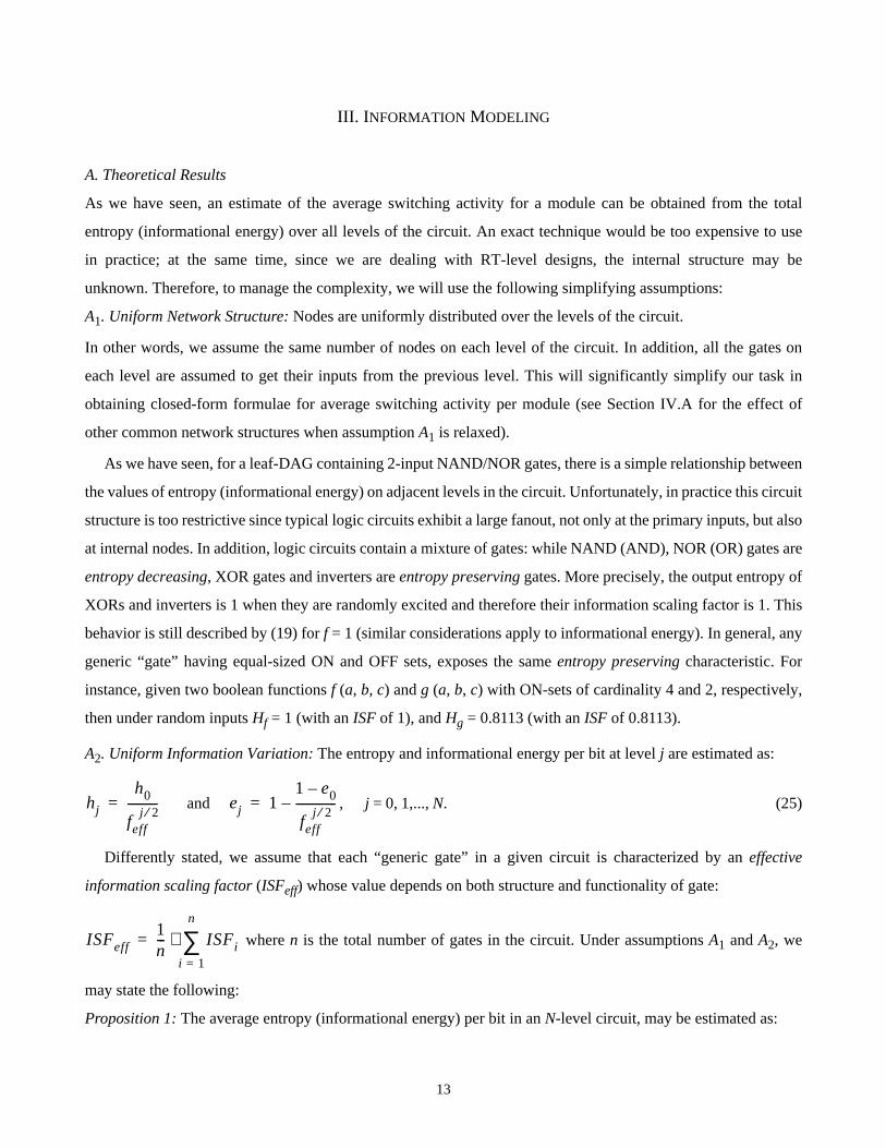
The problem of power estimation at the RT-level is different from that at the logic level: whilst at gate level

it is desirable to determine the switching activity at each node (gate) in the circuit (Fig.1(a)), for RT-level

Pavg

fclk2

--------- VDD2

Cn swn⋅

n∑⋅ ⋅=

3

designs an average estimate per module is satisfactory (Fig.1(b)). In other words, some accuracy may be

sacrificed in order to obtain an acceptable power estimate early in the design cycle at a significantly lower

computational cost.

Fig.1 comes here

In the data-flow graph considered in Fig.1(b), the total power consumption may be estimated as:

. Usually, the interconnect power consumption is either estimated separately or

included in the power consumption of the modules, therefore we can write:

where the summation is performed over the set of modulesM

used in the data-flow graph, and , stand for the capacitance loading and the average switching

activity of modulemj, respectively. Basically, what we propose is to characterize the average switching activity

of a module ( ) through the average switching activity for atypical signal line in that module (swavg).

More formally, for a generic modulemj having n internal lines (each characterized by its capacitance and

switching activity valuesci andswi, respectively), we have:

(2)

We assume that module capacitances are either estimated or taken from a library, therefore we concentrate

on estimating the average switching activity per module. This is a quite different strategy compared to the

previous work. The only other proposed method for power estimation at RT-level is simulative in nature,

requires precharacterization of the modules and may be summarized as follows: first, RT-level simulation is

performed to obtain the average switching activity at the inputs of the modules and then, this switching activity

is used to “modulate” a switched capacitance value (product of the switching activity and the physical

capacitance) which is precomputed and stored for each module in the library to obtain the power dissipation

estimate [14]. Compared to this methodology, the distinctive feature of the present approach, is thatit does not

require simulation; its predictions are based only on the characteristics of the input sequence and some

knowledge about the function and/or structure of the circuit (see Section IV for details).

B. Overview and Organization of the Paper

In this paper, we address the problem of power estimation at the RT-level from an information theoretical

Ptotal Pwires Pmodules+=

Ptotal Pmjmj M∈∑ Cmj

SWmj⋅( )

mj M∈∑∝≈

CmjSWmj

SWmj

Pmjci swi⋅( )

i 1=

n

∑ swavg cii 1=

n

∑⋅≈∝ swavg Cmj⋅=

Cmj

4

point of view [15]. Traditionally, entropy has been considered a useful measure for solving problems of area

estimation, timing analysis [17][18] and testing [19][20]. We propose two new measures for estimating the

power consumption of each module based onentropy and informational energy. Our entropy/informational

energy-based measures simply provide an approximation for the functional activity in the circuit without

having to necessarily simulate the circuit. With some further simplifications, simple closed form expressions

are derived and their value in practical applications is explored.

We should point out that although this paper targets RT-level and behavioral design, it also presents, as a by-

product, a technique applicable to logic level designs. This is a first step in building a unified framework for

power analysis from gate level to behavioral level.

The paper is organized as follows. Sections II and III introduce the main concepts and the motivation behind

our model. In Section IV we present some practical considerations and in Section V, we give the results

obtained by analyzing a common data-path and benchmark circuits. Finally, we conclude by summarizing our

main ideas.

II. THEORETICAL FRAMEWORK

A. An Entropy-Based Approach

Let A1,A2,...,An be a complete set of events which may occur with the probabilitiesp1, p2,..., pn that is:

(3)

Let us consider an experiment where the outcome is unknown in the beginning; such an experiment exposes

a probability finite fieldAn, completely characterized by the discrete probability distributionp1,p2,...,pn. In

order to quantify the content of information revealed by the outcome of such an experiment, Shannon

introduced the concept of entropy [21].

Definition 1: (Entropy)

Entropy of a finite fieldAn (denoted byH (An)) is given by:

(4)

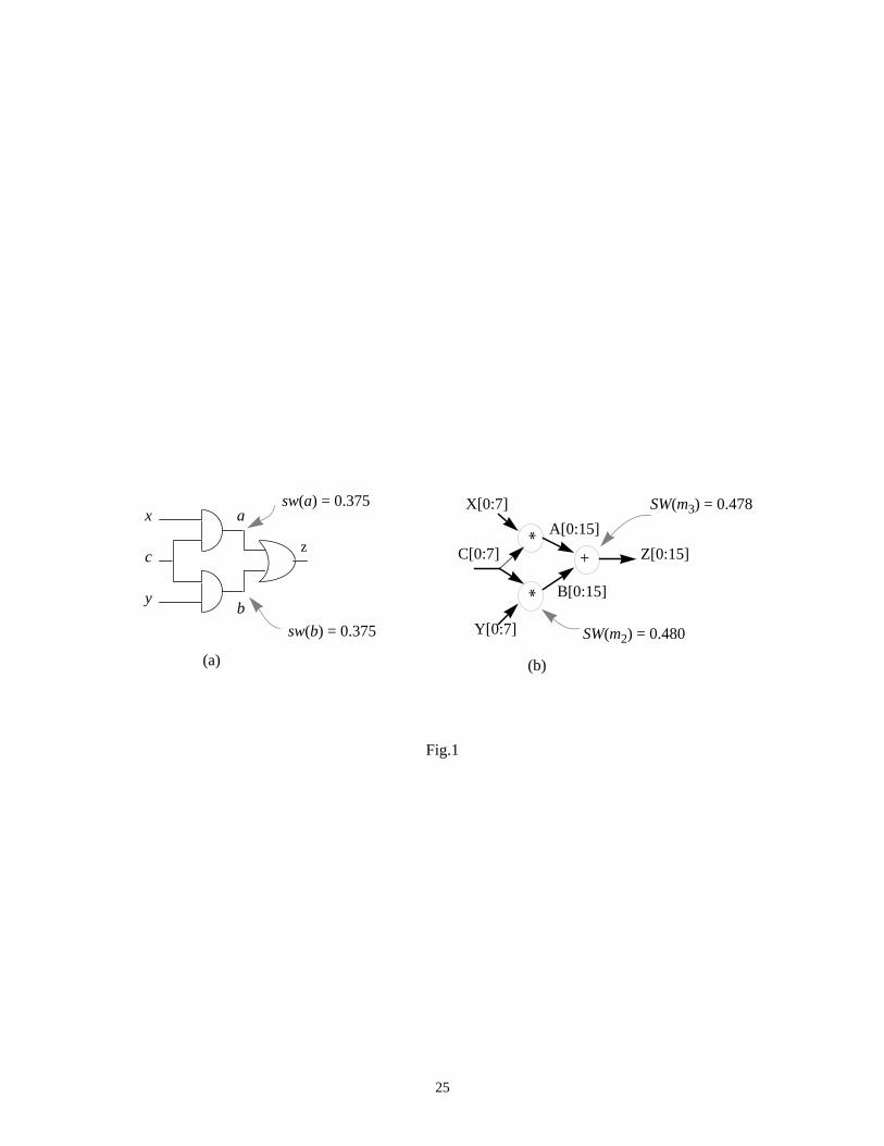
Entropy satisfies some basic properties detailed in [21]. We plot in Fig.2 the entropy of a Boolean variable

as a function of its signal probability, that is .

pk 0≥ k 1 2 … n, , ,= pkk 1=

n

∑ 1=

H An( ) H p1 p2 … pn, , ,( ) pk pklogk 1=

n

∑–= =

H A2( ) p plog⋅– 1 p–( ) 1 p–( )log⋅–=

5

Fig.2 comes here

First, we should note that log (pk) ≤ 0 since 0 < pk ≤ 1 and so H (An) ≥ 0. Thus, the entropy can never be

negative. Second, let p1 = 1, p2 =... = pn = 0. By convention, pk log (pk) = 0 when pk = 0 and hence, in this case,

H (An) = 0. Conversely, H (An) = 0 implies that pk log (pk) = 0 for all k, so that pk is either 0 or 1. But only one

pk can be unity since their sum must be 1. Hence, entropy is zero if and only if there is complete certainty.

Definition 2: (Conditional Entropy)

Conditional entropy of some finite field An with probabilities {pi}1≤i≤n with respect to Bm (with probabilities

{qi}1≤i≤m) is defined as:

(5)

where pkj is the conditional probability of events Aj and Bk (pkj = prob (Aj |Bk)). In other words, conditional

entropy refers to the uncertainty left about An when Bm is known.

Definition 3: (Joint Entropy)

Given two finite fields An and Bm, their joint entropy is defined as:

(6)

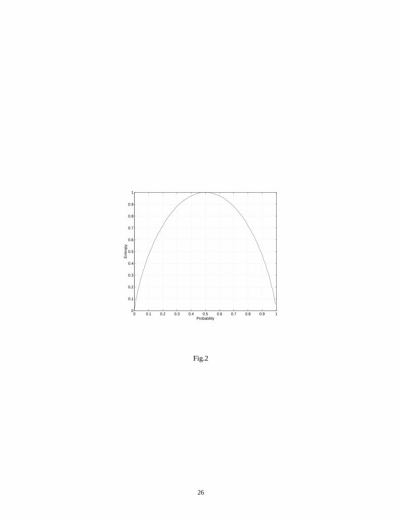
Based on these two concepts, one can find the information shared by two complete sets of events:

which is called mutual information (or transinformation). Moreover, by using the above definitions, one can

show that:

(7)

The Venn diagram for these relations is shown in Fig.3.

Fig.3 comes here

The concept of entropy is equally applicable to partitioned sets of events. More precisely, given a

partitioning ∏ = {A1, A2,..., An} on the set of events, the entropy of this partitioning is:

(8)

H An Bm( ) qk pkj pkj( )log⋅ ⋅k 1=

m

∑j 1=

n

∑–=

H An Bm×( ) qk pkj qk pkj⋅( )log⋅ ⋅k 1=

m

∑j 1=

n

∑–=

I An Bm;( ) H An( ) H Bm( ) H An Bm×( )–+=

I An Bm;( ) H An( ) H An Bm( )–=

H Π( ) p Ai( ) p Ai( )logi 1=

n

∑–=

6

wherep(Ai) is the probability of classAi in partition ∏.

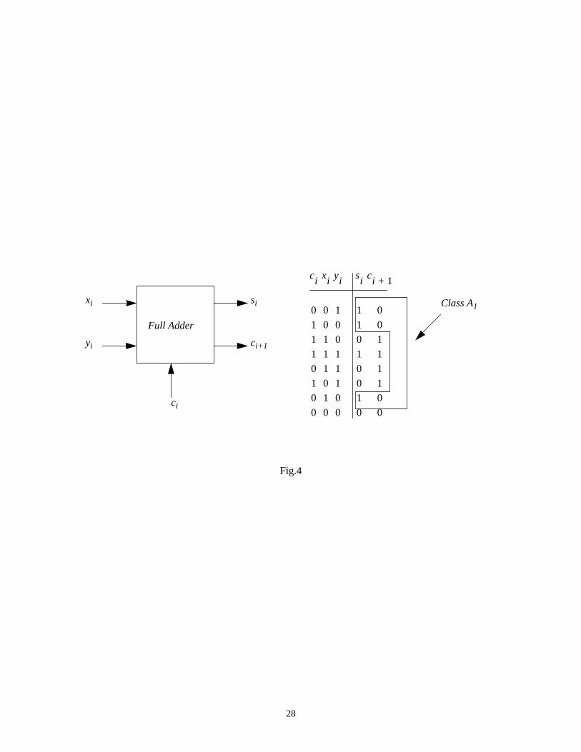
Example 1: The truth table for a randomly excited 1-bit full adder is given below:

Fig.4 comes here

wherexi, yi are the inputs,ci is carry-in,si is the sum bit andci+1 is carry-out. The output space is partitioned in

four classes as∏ = {A1, A2, A3, A4} = {10, 01, 11, 00}, wherep(A1) = p(A2) = 3/8, p(A3) = p(A4) =1/8.

Applying (8) we obtainH(∏) = 1.8113. We observe that within a class there is no activity on the outputs; this

means that output transitions may occur only when one has to cross class boundaries in different time steps. If

the output sequence is purely random, then exactlyH bits are needed to represent the output sequence;

therefore the average number of transitions per word (or average switching activity per word) will beH/2. In

any other nonrandom arrangement, for a minimum length encoding scheme, the average number of transitions

per word will be ≤ H/2, so in practice,H/2 can serve as a conservative upper bound on the number of

transitions per word. In our example, we find an average switching value approximately equal to 0.905 which

matches fairly well the exact value 1 deduced from the above table. Such a measure was suggested initially by

Hellerman to quantify thecomputational work of simple processes [16].

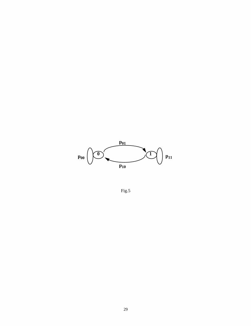
More formally, if a signalx is modelled as a lag-one Markov chain with conditional probabilitiesp00, p01,

p10, p11 and signal probabilitiesp0 andp1 as in Fig.5,

Fig.5 comes here

then we have the following result:

Theorem 1: h (x+|x-) ≥ 2 ·sw (x) · (p00 + p11), whereh (x+|x-) is the conditional entropy between two successive

time steps andsw (x) is the switching activity of linex.

Proof:

According to Definition 2,h (x+|x-) = -p1 (p10 logp10 + p11 logp11) -p0 (p00 logp00 + p01 logp01). The signal

probabilities can be expressed in terms of conditional probabilities as: and ,

respectively [9]. Using the well-known identity for 0 <a < 1, we obtain:

h (x+|x-) = .

p1

p01

p01 p10+---------------------= p0

p10

p01 p10+---------------------=

1 a–( )ln– ak

k-----

k 1=

∞

∑=

12 2( )ln⋅----------------------

2 p01 p10⋅ ⋅p01 p10+

---------------------------p00

k 1–p01

k 1–+

p00⋅ p10

k 1–p11

k 1–+

p11⋅+

k---------------------------------------------------------------------------------------------------------

k 1=

∞

∑⋅ ⋅

7

We note that is exactly the switching activity of line x. The above identity is general, but it is hard

to use in practice in this form; therefore, we try to bound the summation. To begin with, we note that

and that ak-1 + bk-1 (for a + b = 1) is minimized when a = b = 0.5.

Thus, h (x+|x-) ≥ or, using again the above identity, we get:

h (x+|x-) ≥ 2 · sw (x) · (p00 + p11).

■

We have thus obtained an upper bound for the switching activity of signal x when it is modelled as a lag-one

Markov chain. To obtain an upper bound useful in practice, we use the following result:

Corollary 1: Under the temporal independence assumption, we have that sw (x) ≤ h (x) / 2.

Proof:

If we assume temporal independence, that is, p1 = p01 = p11, p0 = p10 = p00 and h (x+|x-) = h (x), then we have:

p00 + p11 = 1 and hence the relationship between sw (x) and h (x) is exactly the one based on intuition: sw (x) ≤

h (x) / 2.

■

To evaluate H, one can use basic results from information theory concerning transmission of information

through a module. More precisely, for a module with input X and output Y, we have

and by symmetry due to the commutativity

property of mutual information. When input X is known, no uncertainty is left about the output Y and thus

H(Y|X) is zero. Therefore, the information transmitted through a module can be expressed as

which represents the amount of information provided about X by Y. For instance,

in Fig.4, I (X; Y) = H (Y) = 3 - 1.1887 = 1.8113; thus, informally at least, the observation of the output of the

module provides 1.8113 bits of information about the input, on average. However, in real examples, this type

of characterization becomes very expensive when the input/output relation is not a one-to-one mapping. This

usually requires a large number of computations; for instance, the exact calculation of the output entropy of an

n-bit adder, would require the knowledge of joint input/output probabilities and a double summation with 22n

terms (as in (5)). As a consequence, in order to analyze large designs, we target a compositional approach

where the basic modules are already characterized in terms of transinformation and what is left to find, is only

a propagation mechanism among them (details are given in Section IV).

2 p01 p10⋅ ⋅p01 p10+

---------------------------

x f x( )⋅ x min f x( )[ ]⋅≥ for x 0≥

12 2( )ln⋅---------------------- sw x( )

p00 p11+( ) 1

2k 2–

-----------⋅

k---------------------------------------------

k 1=

∞

∑⋅ ⋅

I X Y;( ) H X( ) H X Y( )–= I X Y;( ) H Y( ) H Y X( )–=

H Y( ) H X( ) H X Y( )–=

8

As we have seen, an appropriate measure for the average switching activity of each net in the circuit is its

entropy value. Basically, what we need is a mappingξ → ξ’ from the actual setξ of the nets in the target

circuit (each having a possibly distinct switching activity value) to a virtual setξ’ , which contains the same

collection of wires, but this time each net has the same value of switching activity. More formally,ξ → ξ’ is a

mapping such that the following conditions are satisfied:

Bearing in mind this, one can express the total number of transitions per step as:

(10)

wheren stands for the presumed cardinality ofξ’ andh (ξ’) represents the average entropy per bit of any net in

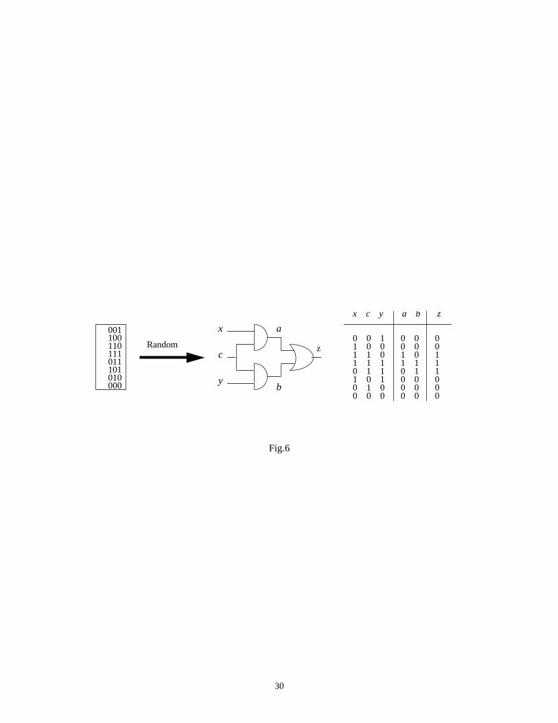
ξ’ . To clarify these ideas, let us consider the simple circuit in Fig.6.

Fig.6 comes here

In this example, we feed the circuit with a 3-bit random sequence and tabulate in the right side, the logic

values obtained in the entire circuit by logic simulation. We have thatξ = {x, c, y, a, b, z} with the switching

profile (in number of transitions) {4, 4, 4, 2, 2, 2}, respectively. Doing a quick calculation, we getSW(ξ) =

2.25 transitions per step. On the other hand,ξ’ = { x, c, y, a, b, z} with the average entropyh (ξ’ ) = (3 * 1 + 2 *

0.811 + 0.954) / 6 = 0.9295 characterizing each signal in the set; using relation (10) we get an expected value

SW(ξ’ ) = 2.73 which is greater thanSW(ξ), but sufficiently close to it.

Unfortunately, in large circuits, it is expensive to computeh (ξ’) as the complete set of events characterizing

a circuit is exponential in the number of nodes. To avoid the brute force approach, that is exhaustive logic

simulation, we make some simplifying assumptions which will be detailed in Section III.A.

B. An Informational Energy-Based Approach

Assuming that we have a complete set of eventsAn (as in (3)), we may regard the probabilitypk as the

information associated with the individual eventAk. Hence, as in the case of entropy, we may define an average

measure for the setAn:

Definition 4: (Informational Energy)

The global information of the finite fieldAn (denoted by E(An)) may be expressed by itsinformational energy

|ξ| = |ξ’|

sw(xi) = sw(xj) for any xi, xj ∈ ξ’ (9)

SW ξ( ) SW ξ'( ) nh ξ'( )

2-------------⋅≤=

9

as (also called theGini Function1):

(11)

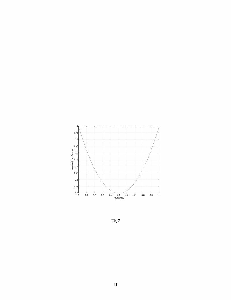
We plot in Fig.7 the informational energy of a Boolean variable as a function of its signal probability, that is

.

Fig.7 comes here

Due to its simplicity, the informational energy was used mainly in statistics (not necessarily in conjunction

with Shannon’s entropy) as a characteristic of a distribution (discrete as is the case here, or continuous in

general). However, without a precise theory, its use was rare until its usefulness was proved in [22].

The value of the informational energy is always upper-bounded by 1. This is because

with equality iff one of the events has probability 1 and the rest of them have the

probability 0. Thus,E (An) = 1 iff the experiment provides the same determinate and unique result. The basic

properties satisfied by the informational energy can be found in [23][24]. We also give the following definition:

Definition 5: (Conditional Informational Energy)

Conditional informational energy of some finite fieldAn with probabilities {pi} 1≤i≤n with respect toBm (with

probabilities {qi} 1≤i≤m) is defined as:

(12)

wherepkj is the conditional probability of eventsAj andBk.

Based on this measure, one can find a relationship between the switching activity and the informational

energy. Lete(x) denote the informational energy of a single bitx. Consideringx modelled as a lag-one Markov

chain with conditional probabilitiesp00, p01, p10, p11 and signal probabilitiesp0 andp1 as in Fig.5, we can give

the following result:

Theorem 2: e (x+|x-) = 1 - sw (x) · (p00 + p11) wheree (x+|x-) is the conditional informational energy between

two successive time steps.

1This was first used by Corrado Gini in a study from “Atti del R. Ist. Veneta di Scienze,”Lettere ed Arti, 1917, 1918, v. LXXVII

E An( ) pj2

j 1=

n

∑=

E A2( ) p2

1 p–( ) 2+=

pj2

j 1=

n

∑ pjj 1=

n

∑ 2

1=≤

E An Bm( ) qk pkj2⋅

k 1=

m

∑j 1=

n

∑=

10

Proof:

From Definition 5, e (x+|x-) = p1 (p102 + p11

2) +p0 (p002 + p01

2). Since the switching activity of line x is

and , one can write the following relationship between

conditional informational energy and switching activity:

■

In the most general case, p00 and p11 can take any values and thus even if we have an exact relation between

energy and switching activity (i.e. sw (x) = (1 - e (x+|x-)) / (p00 + p11)) we cannot bound the sum from the

denominator. However, under the temporal independence assumption, we have an exact relation since p00 + p11

= 1 and thus:

Corollary 2:

. (13)

■

For instance, returning to the 1-bit full-adder example in Fig.4, we find Einput = 0.125 and Eoutput = 0.875.

Thus, on average, the output exposes an informational energy of 0.437 and, based on (13), a switching activity

of 0.563 (compared to the exact value of 0.5). Thus, informational energy (along with entropy) seems to be a

reliable candidate for estimation of energy consumption.

Once again we consider the virtual mapping ξ → ξ’, where each net in ξ’ is characterized by the same

amount of average informational energy e (ξ’). Based on (9), the expected switching activity per step in the

whole circuit SW (ξ’), can be expressed as:

(14)

where the cardinality of ξ’ is assumed to be n.

Considering the simple case in Fig.6, we get e (ξ’) = (3 * 0.5 + 2 * 0.625 + 0.531) / 6 = 0.546 and therefore,

SW (ξ’) = 2.71 which matches well the actual value (2.25). However, in real circuits, direct computation of e

(ξ’) is very costly; to develop a practical approach, we need further simplifications as will be shown

subsequently.

2 p01 p10⋅ ⋅p01 p10+

--------------------------- p1

p01

p01 p10+---------------------= p0

p10

p01 p10+---------------------=

e x+

x–

p01 p10

2p11

2+

⋅ p10 p002

p012

+ ⋅+

p01 p10+----------------------------------------------------------------------------------------= =

p01 1 2 p10 p11⋅ ⋅–( )⋅ p10 1 2 p00 p01⋅ ⋅–( )⋅+

p01 p10+--------------------------------------------------------------------------------------------------------------------- 1 sw x( ) p00 p11+( )⋅–= =

sw x( ) 2p x( ) 1 p x( )–( ) 1 e x( )–= =

SW ξ( ) SW ξ'( )= n 1 e ξ'( )–( )⋅=

11

C. Quantitative Evaluations

In order to derive a consistent model for energy consumption at the RT-level, we first have to abstract

somehow the information which is present at the gate level. Thus, a simplified model is adopted as a starting

point.

Let us consider some combinational block realized on n levels as a leaf-DAG1 of 2-input NAND gates (a

similar analysis can be carried out for 2-input NOR gates and the final result is the same). We assume that

inverters may appear only at primary inputs/outputs of the circuit; we do not include these inverters in the level

assignment step. One can express the signal probability of any net at level j+1 as a function of the signal

probability at level j by:

(15)

Similarly, the signal probability of any net at level j+2 is given by:

(16)

The average entropy per net at level j is given by:

(17)

Using the corresponding average entropy per net at level j+2, the parametrized relationship between hj and hj+2

can be approximated by when j is sufficiently large (values greater than 6). Hence we get

expressions for entropy per bit at even/odd levels of the circuit: and , where h0, h1 are

entropies per bit at the primary inputs and first level, respectively. To get a closed form expression, we may

further assume that h1 may be estimated in terms of h0 as (in fact, the exact entropy decrease for a

NAND gate excited by pseudorandom inputs is 0.8113, but for uniformity, we use ). Thus, for a

2-input NAND gate leaf-DAG, the entropy per bit at level j may be approximated as:

(18)

This may be further generalized for the case of f-input NAND gate leaf-DAGs, observing that increasing the

1In a leaf-DAG, only the leaf nodes have multiple fanouts.

pj 1+ 1 pj2

–= j∀ 0 …, n 1–,=

pj 2+ 1 1 pj2

– 2

–= j∀ 0 …, n 2–,=

hj pj pjlog⋅– 1 pj–( ) 1 pj–( )log⋅–=

hj 2+

hj

2----≈

h2j

h0

2j

-----≈ h2j 1+

h1

2j

-----≈

h1

h0

2-------≈

1

2------- 0.707=

hj

h0

2j 2⁄---------≈

12

fanin from 2 to f, produces a decrease in the number of levels by log (f). Hence, for a fanin of f, (18) becomes:

(19)

Definition 6: We call the information scaling factor (ISF); it characterizes each logic component (gate,

module or circuit).

We will see how relation (19) is affected by the circuit structure and functionality in general. In any case,

this provides a starting point for estimating the total entropy at each level in the circuit. In general, the total

entropy over all levels N in the circuit is given as:

(20)

where Hj is the total entropy at level j and nj is the number of nodes on level j.

All these considerations can be easily extended for the case of informational energy. Considering the same

assumptions as in previous section and using relation (15), the informational energy per net at level j may be

expressed as:

(21)

Applying (15) for level j+2 and substituting in (21), we get the following parameterized dependency

between the informational energies at levels j + 2 and j:

(22)

Using a similar approach as in the case of entropy, we get the following expression for the average

informational energy per bit at level j in a circuit with fanin f:

(23)

From here, an estimate can be drawn for the total energy at level j, and thus for the total energy over all the

levels of the circuit:

(24)

where Ej is the total energy at level j and again nj is the number of nodes on level j.

hj

h0

2j flog⋅( ) 2⁄-------------------------≈

h0

fj 2⁄----------=

1

f-----

Htotal Hjj 0=

N

∑ nj hj⋅j 0=

N

∑= =

ej pj2

1 pj–( ) 2+=

ej 2+ 1 1 pj2

– 2

– 2

1 pj2

– 4

+=

ej pj2

1 pj–( ) 2+=

ej 11 e0–

fj 2⁄--------------–=

Etotal Ejj 0=

N

∑ nj ej⋅j 0=

N

∑= =

13

III. I NFORMATION MODELING

A. Theoretical Results

As we have seen, an estimate of the average switching activity for a module can be obtained from the total

entropy (informational energy) over all levels of the circuit. An exact technique would be too expensive to use

in practice; at the same time, since we are dealing with RT-level designs, the internal structure may be

unknown. Therefore, to manage the complexity, we will use the following simplifying assumptions:

A1. Uniform Network Structure: Nodes are uniformly distributed over the levels of the circuit.

In other words, we assume the same number of nodes on each level of the circuit. In addition, all the gates on

each level are assumed to get their inputs from the previous level. This will significantly simplify our task in

obtaining closed-form formulae for average switching activity per module (see Section IV.A for the effect of

other common network structures when assumptionA1 is relaxed).

As we have seen, for a leaf-DAG containing 2-input NAND/NOR gates, there is a simple relationship between

the values of entropy (informational energy) on adjacent levels in the circuit. Unfortunately, in practice this circuit

structure is too restrictive since typical logic circuits exhibit a large fanout, not only at the primary inputs, but also

at internal nodes. In addition, logic circuits contain a mixture of gates: while NAND (AND), NOR (OR) gates are

entropy decreasing, XOR gates and inverters areentropy preserving gates. More precisely, the output entropy of

XORs and inverters is 1 when they are randomly excited and therefore their information scaling factor is 1. This

behavior is still described by (19) forf = 1 (similar considerations apply to informational energy). In general, any

generic “gate” having equal-sized ON and OFF sets, exposes the sameentropy preserving characteristic. For

instance, given two boolean functions f (a, b, c) andg (a, b, c) with ON-sets of cardinality 4 and 2, respectively,

then under random inputsHf = 1 (with anISF of 1), andHg = 0.8113 (with anISF of 0.8113).

A2. Uniform Information Variation: The entropy and informational energy per bit at levelj are estimated as:

and , j = 0, 1,...,N. (25)

Dif ferently stated, we assume that each “generic gate” in a given circuit is characterized by aneffective

information scaling factor (ISFeff) whose value depends on both structure and functionality of gate:

wheren is the total number of gates in the circuit. Under assumptionsA1 andA2, we

may state the following:

Proposition 1: The average entropy (informational energy) per bit in anN-level circuit, may be estimated as:

hj

h0

feffj 2⁄----------= ej 1

1 e0–

feffj 2⁄--------------–=

ISFeff1n--- ISFi

i 1=

n

∑⋅=

14

(26)

wherehin (ein), hout (eout) are the average input and output entropies (energies) per bit1.

Proposition 1 gives us an estimate of the average entropy/informational energy in a circuit withN levels. The

factorfeff is “hidden” in the relationship betweenN, hin (ein) andhout (eout) since the outputs are assumed to be on

level N:

(27)

The above equations show that the loss of information per bit from one level to the next decreases with the

number of levels. For circuits with a large logical depth, one can obtain from (26) simpler equations by lettingN

approach infinity. This is also useful in cases where information about the logic depth of the circuit is not readily

available. We therefore make the following assumption:

A3. Asymptotic Network Depth: The number of levelsN is large enough to be considered infinity (N → ∞). Using

this assumption, we get the following:

Corollary 3: For sufficiently large N, the average entropy and informational energy per bit in the circuit are given

by:

(28)

1Proofs that are omitted here can be found in [24].

havg hin

1hout

hin---------

N 1+N

-------------

–

N 1+( ) 1hout

hin---------

1N----

–

⋅

------------------------------------------------------------⋅=

eavg 1 1 ein–( )–

11 eout–

1 ein–------------------

N 1+N

-------------

–

N 1+( ) 11 eout–

1 ein–------------------

1N----

–

⋅

---------------------------------------------------------------------⋅=

hout hN

h0

feffN 2⁄----------

hin

feffN 2⁄----------= = =

eout eN 11 e0–

feffN 2⁄--------------– 1

1 ein–

feffN 2⁄---------------–= = =

havg

hin hout–

hin

hout---------ln

----------------------= eavg 1ein eout–

1 eout–

1 ein–------------------ln

------------------------–=

15

Note: In the above derivations, trivial cases such as a value of zero for the input or output entropy and a value of

one for the input or output energy are excluded.

What we have obtained so far are simple formulae for estimating the average entropy (informational energy)

per bit, and from these, the average switching activity over all the nets in the module. The main difficulty in

practice is to estimate the actual output entropy hout (or informational energy eout) since the information usually

available at this level of abstraction is not detailed.

B. The Influence of Structure and Functionality

All logic gates belonging to a given module can be characterized by an effective factor feff which captures

information about the circuit structure and functionality. How can we model a general circuit for entropy/

energy based evaluations? One can consider relations (26) and (27), where the information scaling factor

reflects not only the structure, but also the fraction of information preserving gates.

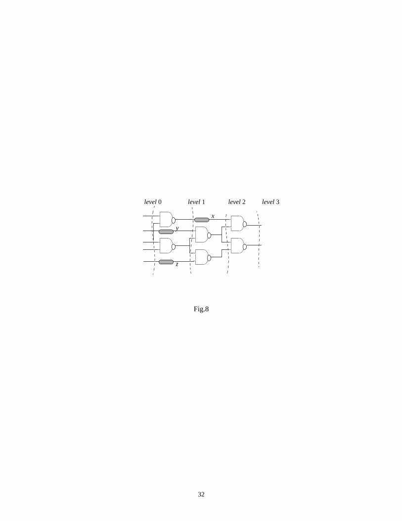
Example 2: Let us consider for instance, circuit C17 given below.

Fig.8 comes here

To levelize it properly (every wire that connects the output of a gate at level i to the input of a gate at level

i+2 must go through some buffer gate at level i+1), we added three “dummy” components x, y, z. Logically, x,

y, z function as buffers but informationally, they are entropy preserving elements. Considering the nodes

uniformly distributed throughout the circuit (according to assumption A1), the average number of nets per level

is 4.25. Applying random vectors at the circuit inputs, the exact value of the entropy per bit at the output is

obtained as hout = 0.44. The effective scaling factor can be calculated as a weighted sum over all the gates in

the circuit; thus the corresponding feff is 1.55 (there are 3 entropy preserving and 6 entropy decreasing gates).

From (27) we get an estimate for the output bit entropy (j = 3) as hout = 0.51 which is reasonably close to the

exact value. Based on the input and output entropy, we may get an estimate for the average entropy per bit and

thus for the switching activity. The average switching activity for a generic net in the circuit is swavg(sim) =

0.437 (from simulation) and based on (26), we get swavg(est) = 0.382 which is very good compared to

simulation. A similar analysis can be performed for the informational energy.

IV. PRACTICAL CONSIDERATIONS

A. Using Structural Information

These considerations are equally applicable to data-path operators with known internal structure as well as to

16

control circuits represented either at gate or RT-level.

If some structural information is available (such as the number of internal nodes, the number of logic

levels), the average entropy (informational energy) may be evaluated using the actual values of feff, N and the

distribution of nodes on each level. In all cases, the output entropy (informational energy) is the same,

computed as in (27). The average entropy (or informational energy) for the whole module depends on the

actual distribution of nodes in the circuit. In practice, some common distributions are:

a) Uniform distribution (this case was treated in detail in Section III).

b) Linear distribution (e.g. circuit C17 in Fig.8):

In this case, using a similar approach as the one in Section III, we found the following result (valid for N →

∞) for a generic n input, m output module:

(29)

c) Exponential distribution (e.g. a balanced tree circuit with 8 inputs):

In this case, we have for N → ∞:

(30)

Note: The main advantage of equations (29), (30)1 is that they allow an estimate of average entropy (and

therefore of average switching activity) of modules or gate-level circuits, without resorting to logic simulation

or probabilistic techniques like those presented in [3]-[9].

Similar derivations apply for informational energy. We can see that when n = m, we get the same results as

in Section III (see equation (28)).

B. Using Functional Information

For common data-path operators, can be efficiently estimated based on the “compositional technique”

introduced in [20]. There, the Information Transmission Coefficient (ITC) is defined as the fraction of

information that is transmitted through a function; it may be computed by taking the ratio of the entropy on the

outputs of a function and the entropy on the inputs of that function. For convenience, we call ITCs “Entropy

1More general expressions for (29), (30) (i.e. when N is not approaching infinity) can be found in [24].

havg

2 n hin⋅ ⋅

n m+( )hin

hout---------

ln⋅----------------------------------------------- 1

mn----

hout

hin---------⋅

1 mn----–

1hout

hin---------–

⋅

hin

hout---------

ln

--------------------------------------------------––

⋅=

havg

hinnm----

ln⋅

1 mn----–

----------------------------

1m hout⋅n hin⋅

------------------–

n hin⋅m hout⋅------------------

ln

-------------------------------⋅=

17

Transmission Coefficients” (HTCs) and we characterize them as follows:

(31)

where Win (Wout) is the number of bits on the input (output) and hin (hout) is the input (output) average bit

entropy.

Therefore, the output entropy hout is estimated based solely on the RT-level description of the circuit

through a postorder traversal of the circuit. The main advantage of such an approach, is that it needs only a

high-level view of the design in order to derive useful information.

A similar technique can be introduced to compute the output informational energy as follows.

Definition 7: (Energy Transmission Coefficient)

The fraction of informational energy transmitted through a function called “Energy Transmission Coefficient”

(ETC) is defined as the ratio of the output and input informational energy.

In Table 1 we give the values of the ETC coefficients for the same data-path operators considered in [20].

Table 1 comes here

Similar to (31), we may evaluate ETCout as a function of ETC for the component of interest and the ETC

values for all inputs:

(32)

where ein (eout) is the input (output) average bit informational energy.

Common data-path circuits (e.g. arithmetic operators) have the scalability property, that is, their HTC/ETC

values do not depend significantly on the data-path width. Unfortunately, there are many other circuits (e.g.

control circuits) which cannot be treated in this manner. In those cases, relations (28), (29) and (30) have to be

used in conjunction with some information about the circuit structure in order to get reliable estimates for

average switching activity.

C. HTC and ETC Variations with the Input Statistics

As presented in [20], Thearling and Abraham’s compositional techniques is only an approximation because it

does not consider any dependency which may arise in practical examples. In reality, every module may be

embedded in a larger design and therefore its inputs may become dependent due to the structural dependencies

(namely, the reconvergent fan-out) in the preceding stages of the logic. As a consequence, the values given in

HTCcomp Wout

Win-----------

hout

hin---------⋅=

ETCcomp Wout

Win-----------

eout

ein---------⋅=

18

[20] or here in Table 1 (which correspond to the case of pseudorandom inputs) result in large errors as we

process a circuit with internal reconvergent fan-out. To be accurate we need a more detailed analysis as will be

described in the following.

Without loss of generality, we restrict ourselves to the case of 8- and 16-bit adders and multipliers (denoted

below by add and mul, respectively) and for each of them, we consider two scenarios:

- Each module is fed by biased input generators, that is input entropy (informational energy) per bit varies

between 0 and 1 (respectively 0.5 and 1); each such module is separately analyzed.

- Modules are included in a large design with reconvergent fanout branches, so that inputs of the modules

cannot be considered independent. Details of this experiment are reported in [24]. As shown there, the

dependence of HTCs and ETCs on the input statistics can be described empirically by the following simple

relations:

(33)

where the 0-subscripted values correspond to the pseudorandom case (reported in [20] and here in Table 1).

These equations can be easily used to adjust the HTC/ETC coefficients in order to analyze large designs more

accurately. Differently stated, using equations (33) we loose less information when traversing the circuit from

one level to next because we account for structural dependencies.

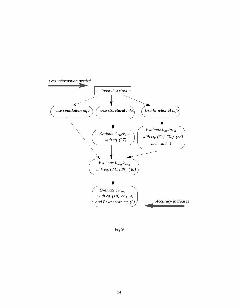
In any case, our proposed framework is also open to simulation (the zero-knowledge scenario); this may

provide accurate values for output entropy (informational energy) values, but with a much higher

computational cost. In practice, we thus have the following options to analyze a logic- or RT-level design:

Fig.9 comes here

In general, using structural information can provide more accurate results either based on entropy or

informational energy measures; supporting evidence for this claim is given in [24]. On the other hand,

evaluations based on functional information require less information about the circuit and therefore may be

more appealing in practice as they provide an estimate of power consumption earlier in the design cycle. The

structural approach is thus more appropriate to be used when a gate-level description is available (and therefore

detailed information can be extracted) whilst the functional approach (using the compositional technique) is

more suitable for RT/behavioral level descriptions.

HTCadd

HTC0add 2 hin–( )⋅≈ HTC

mulHTC0

mul 2hin 1–

⋅≈

ETCadd

ETC0add≈ ETC

mulETC0

mul≈

19

V. EXPERIMENTAL RESULTS

In order to asses the accuracy of the proposed model, two experiments were performed: one involving

individual modules (ISCAS’85 benchmarks and common data-path components) and the other involving a

collection of data-path modules specified by a data flow graph.

A. Validation of the Structural Approach (Gate-Level Descriptions)

The experimental setup consisted of a pseudorandom input generator feeding the modules under

consideration. The values of the entropy and informational energy for the circuit inputs were extracted from the

input sequence, while the corresponding values at the circuit outputs and the average values of entropy or

informational energy were estimated as in Section III (using structural information). These average values were

then used to estimate the average switching activity per node; the latter, when weighted by an average module

capacitance, is a good indicator of power/energy consumption.

We report in Table 2 our results on benchmark circuits and common data-path operators. Powersim and swsim

are the exact values of power and average switching activity obtained through logic simulation under SIS

( and , where k is the number of

primary inputs and gates in the circuit). In the third column, Cmodule stands for the module capacitance

. We also report for comparison under the Powerapprox column the value of power

obtained using the approximation in (2). The error introduced by this approximation (under pseudorandom input

data) is on average 4.56%1. In the next four columns we report our results for average switching activity and

power calculated as in (2) for both entropy- and informational energy-based approaches.

Table 2 comes here

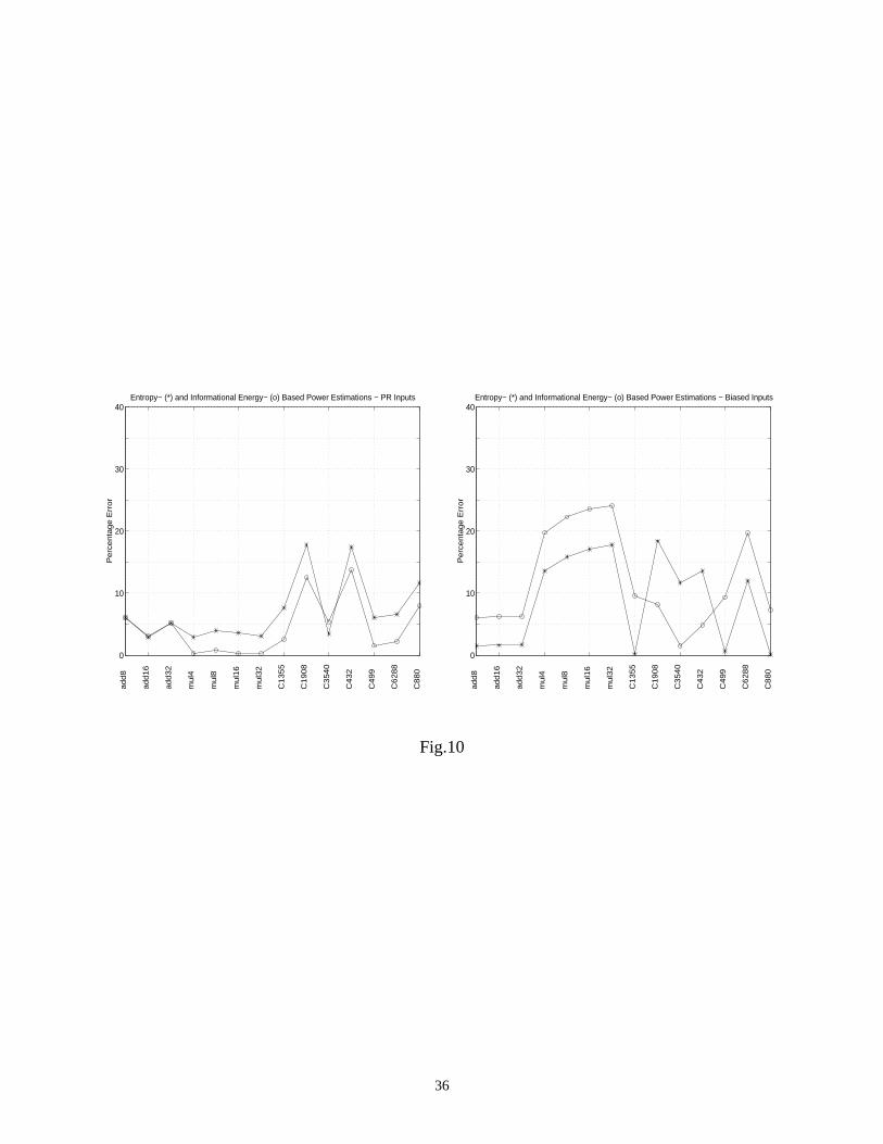
As we can easily see, the average percentage error (over all the circuits) is 11.38% (7.71%) for entropy

(informational energy)-based evaluations of average switching activity, whilst for total power estimation it is

7.03% (4.42%) for entropy (informational energy)-based approaches. These results were found to be consistent

for different input signal probabilities. For comparison, in Fig.10, we present the percentage error variation

obtained for a pseudorandom and a biased input sequence. In the latter case, the average percentage error was

1The percentage error was calculated as .

Powersim12--- VDD

2fclk swsim

iCgate

i⋅i 1=

k

∑⋅ ⋅ ⋅= swsim1k--- swsim

i

i 1=

k

∑⋅=

Cmodule Cgatei

i 1=

k

∑=

valuesim valueest–

valuesim------------------------------------------------ 100⋅

20

11.17% (15.91%) for entropy (informational energy) power estimations. All results were generated in less than

two seconds of CPU time on a SPARC 20 workstation with 64 MBytes of memory.

Fig.10 comes here

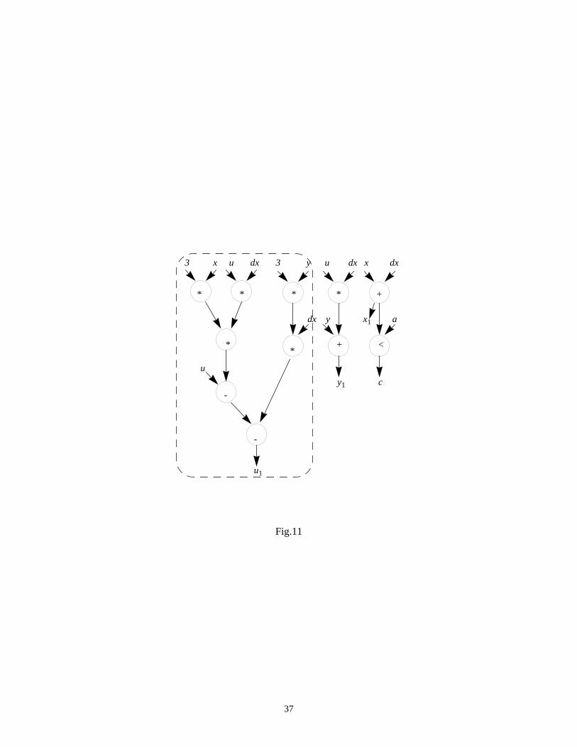
B. Validation of the Functional Approach (Data-Flow Graph Descriptions)

In Fig.11 we consider a complete data-path represented by the data-flow graph of the differential equation

solver given in [25]. All the primary inputs were considered as having 8 bits and the output entropy of the

entire module was estimated with the compositional technique based onHTCs orETCs. TheHTC/ETC values

for the multipliers and adders were calculated according to (33). Using the entropy based approach, the average

switching activity was estimated as 0.1805, whilst when using the informational energy, the average switching

activity was 0.1683. These estimations should be compared with the exact value of 0.1734 obtained by

behavioral simulation.

Fig.11 comes here

Our technique can also be applied to analyze different implementations of the same design in order to trade-

off power for area, speed or testability. Suppose we select from the data-path in Fig.11 only the part which

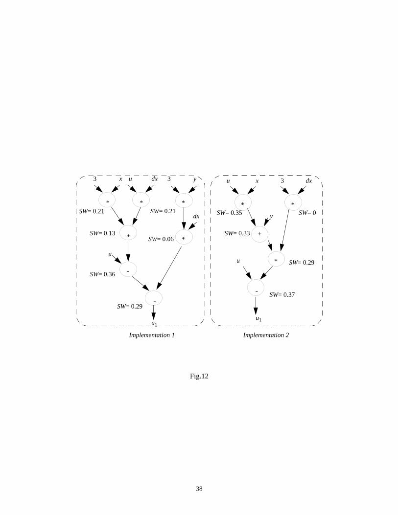
computesu1. In Fig.12 we give two possible implementations of the selected part of the data-path. One is the

same as above and the other is obtained using common algebraic techniques such as factorization and common

subexpression elimination. All the primary inputs were assumed to be random (except inputs ‘3’ and ‘dx’

which are constants). Each adder or multiplier is labelled with its average switching activity valueSW. In the

first case, applying the compositional technique based on entropy, we obtain an average switching activity of

0.186, whilst using informational energy this value is 0.197. For the second implementation, the corresponding

values are 0.242 from entropy and 0.282 from informational energy which show an average increase in

switching activity of 30%. However, considering the module capacitance of adders and multipliers (as given in

Table 2), we actually get a total switched capacitance of 331.15 for the first design and 268.88 for the second

one (using entropy-based estimations). This means a decrease of 19%, and thus, the second design seems to be

a better choice as far as power consumption is concerned.

Fig.12 comes here

C. Limitations of the Present Approach

The simplifying assumptions considered in Sections II and III were aimed at making this approach

predictive in nature. However, they introduce as a side effect some inherent inaccuracies. Generally speaking,

21

simple network structure, uniform information variation and asymptotic network depth are reasonable

hypotheses which perform well on average, but may not be satisfied for some circuits.

On the other side, we do not consider temporal correlations at the modules inputs and in some cases this

could compromise the accuracy of the predictions, mostly for switching activity estimates. Our preliminary

experiments show that the temporal effects are not as important at RT-level as they are at circuit or gate-level

but undoubtfully, the overall quality of the approach would benefit from incorporating them into analysis.

Moreover, using the functional information through HTC/ETCs coefficients as suggested in Section IV, is

applicable only to modules that perform a single well-defined function; multifunctional modules like complex

ALU's would require a more elaborate analysis than the one presented here.

Lastly, our model is intended only for zero-delay model; a general delay model cannot be supported in a

straightforward manner by this information theoretic approach.

VI. CONCLUSION

In this paper, we presented an information theoretic approach for power estimation at the RT and gate

levels of design abstraction. Noting that entropy characterizes the uncertainty of a sequence of applied input

vectors and is thus intuitively related to the input switching activity, we have mathematically shown that (under

temporal independence assumption) the average switching activity of a signal line is upper-bounded by one-

half of its entropy. We then presented two techniques for calculating the entropy at the circuit outputs from the

input entropies.

The first technique, which is more applicable when some information about the circuit implementation is

provided, calculates the output entropy using an effective information scaling factor (derived from the number

and type of logic gates used) and the number of logic levels in the circuit. This technique requires parsing the

circuit netlist to generate the appropriate parameters but otherwise, relies on closed form expressions for power

estimation from that point on.

The second techniques, which is more applicable when only functional/data-flow information about the

circuit is given, calculates the output entropies using a compositional technique. It has linear complexity in the

size of the high-level specification of the circuit and is based on a precharacterization of library modules in

terms of their entropy transmission coefficients.

Having obtained the output entropies, the average entropy per signal line in the circuit is calculated using

closed form expressions derived for three different types of gate distribution per logic level (uniform, linear and

exponential). Finally, the average entropies were used to estimate the average switching activity characterizing

the module under consideration.

22

Similar techniques, were developed and presented for informational energy, which is yet another

information theoretic measure related to the switching activity in the circuit.

Results obtained for common benchmarks show that the proposed power estimation techniques are

extremely fast (few CPU seconds), yet sufficiently accurate (12% relative error on average) to be of use in

practical cases.

REFERENCES

[1] F. N. Najm, ‘A Survey of Power Estimation Techniques in VLSI circuits’, IEEE Transactions on VLSI Systems,vol.2, no.4, pp. 446-455, Dec.1994.

[2] M. Pedram, ‘Power Minimization in IC Design: Principles and Applications’, in ACM Transactions on DesignAutomation of Electronic Systems, vol.1, no.1, pp.1-54, Jan.1996

[3] F.N. Najm, ‘A Monte Carlo Approach for Power Estimation’, IEEE Transactions on VLSI Systems, vol.1, no.1,pp. 63-71, Mar. 1993.

[4] B.J.George, D.Gossain, S.C.Tyler, M.G.Wloka, and G.K.Yeap, ‘Power Analysis and Characterization for Semi-Custom Design’, in Proc. Intl. Workshop on Low Power Design, pp.215-218, April 1994.

[5] C.X.Huang, B.Zhang, A.-C.Deng, and B.Swirski, ‘The Design and Implementation of PowerMill’, in Proc. Intl.Workshop on Low Power Design, pp.105-110, April 1995

[6] A. Ghosh, S. Devadas, K. Keutzer, and J. White, ‘Estimation of Average Switching Activity in Combinationaland Sequential Circuits’, in Proc. ACM/IEEE Design Automation Conference, pp. 253-259, June 1992.

[7] F. N. Najm, ‘Transition Density: A New Measure of Activity in Digital Circuits’, IEEE Transactions on CAD,vol. 12, no. 2, pp. 310-323, Feb. 1993.

[8] C.-Y. Tsui, M. Pedram, and A. M. Despain, ‘Efficient Estimation of Dynamic Power Dissipation with anApplication’, in Proc. IEEE/ACM Intl. Conference on Computer Aided Design, pp. 224-228, Nov. 1993.

[9] R. Marculescu, D. Marculescu, and M. Pedram, ‘Efficient Power Estimation for Highly Correlated InputStreams’, in Proc. ACM/IEEE Design Automation Conference, pp. 628-634, June 1995.

[10] A. Chandrakasan, et. al, ‘HYPER-LP: A System for Power Minimization Using Architectural Transformation’, inProc. IEEE/ACM Intl. Conference on Computer Aided Design, pp. 300-303, Nov.1992.

[11] R. Mehra, J. Rabaey, ‘High Level Estimation and Exploration’, in Proc. Intl. Workshop on Low Power Design,pp.197- 202, April 1994.

[12] P. Landman, J. Rabaey, ‘Power Estimation for High Level Synthesis’, in Proc. European Design AutomationConference, pp. 361-366, Feb.1993.

[13] N. Weste and K Eshraghian, ‘Principles of CMOS VLSI Design: A Systems Perspective’, 2nd Edition, Addison-Wesley Publishing Co., 1994.

[14] P. Landman and J. Rabaey, ‘Black-Box Capacitance Models for Architectural Power Analysis’, in Proc.Intl.Workshop on Low Power Design, pp. 165-170, April 1994.

[15] L. Brillouin, ‘Science and Information Theory’, Academic Press, New York, 1962.

[16] L. Hellerman, ‘A Measure of Computational Work’, in IEEE Trans. on Computers, vol. C-21, No.5, pp. 439-446,1972.

[17] R.W. Cook, M.J. Flynn, ‘Logical Network Cost and Entropy’, in IEEE Trans. on Computers, vol. C-22, No. 9, pp.823-826, Sept. 1973.

[18] K.-T. Cheng, V. Agrawal, ‘An Entropy Measure for the Complexity of Multi-Output Boolean Functions’, in Proc.ACM/IEEE Design Automation Conference, pp. 302-305, June 1990.

[19] V. Agrawal, ‘An Information Theoretic Approach to Digital Fault Testing’, in IEEE Trans. on Computers, vol. C-30, No. 8, pp. 582-587, Aug. 1981.

[20] K. Thearling, J. Abraham, ‘An Easily Computed Functional Level Testability Measure’, in Proc. Intl. TestConference, pp. 381-390, 1989.

23

[21] A. Papoulis, ‘Probability, Random Variables, and Stochastic Processes’, McGraw-Hill Co., 1984.

[22] O. Onicescu, ‘Theorie de l’information. Energie informationelle’, Paris, C.R. Acad.Sci., Tome 263, 1966.

[23] O. Onicescu, V. Stefanescu, ‘Elements of Informational Statistics with Applications’, in Romanian, Bucharest1979.

[24] D. Marculescu, R. Marculescu, and M. Pedram, ‘RT-Level Power Analysis Using Information TheoreticMeasures’, USC Technical Report CENG 95-25, Dec. 1995

[25] P. Paulin, and J. Knight, ‘Force-directed Scheduling for the Behavioral Synthesis of ASICs’, IEEE Transactionson CAD, vol. CAD-8, No. 6, pp. 661-679, July 1989.

24

List of figures and tables captions:

Fig.1: Power estimation issues at the logic and RT-levels

Fig.2: Entropy H(A2) vs. probability

Fig.3: A set-theoretic representation of different entropies

Fig.4: 1-bit full adder

Fig.5: A two-state Markov-chain modelling a signal line x

Fig.6: An example to illustrate the mapping ξ → ξ’

Fig.7: Informational energy E(A2) vs. probability

Fig.8: An example of levelization - circuit C17

Table 1: ETC values for common data-path operators

Fig.9: Flowchart of the power estimation procedure

Table 2: Data-path and ISCAS’85 circuits (All power values are computed using VDD = 5V and fclk = 100MHz)

Fig.10: Percentage error for power estimations under PR and biased inputs

Fig.11: A data-path example

Fig.12: Comparison between two possible implementations

25

Fig.1

+

**

c

x

y

a

b

z

X[0:7]

Y[0:7]

Z[0:15]

A[0:15]

B[0:15]

sw(a) = 0.375

sw(b) = 0.375 SW(m2) = 0.480

(a) (b)

SW(m3) = 0.478

C[0:7]

26

Fig.2

0 0.1 0.2 0.3 0.4 0.5 0.6 0.7 0.8 0.9 10

0.1

0.2

0.3

0.4

0.5

0.6

0.7

0.8

0.9

1

Probability

En

tro

py

27

Fig.3

I(x; y)

H(x| y) H(y|x)

H(x, y)

28

Fig.4

xi

yi

ci

si

ci+1

Full Adder

ci xi yi si ci 1+

0 0 1 1 0

1 0 0 1 0

1 1 0 0 1

1 1 1 1 1

0 1 1 0 1

1 0 1 0 1

0 1 0 1 0

0 0 0 0 0

Class A1

29

Fig.5

0 1

p01

p10

p11p00

30

Fig.6

c

x

y

a

b

001100110111011101010000

zRandom

x c y a b z

0 0 1 0 0 01 0 0 0 0 01 1 0 1 0 11 1 1 1 1 10 1 1 0 1 11 0 1 0 0 00 1 0 0 0 00 0 0 0 0 0

31

Fig.7

0 0.1 0.2 0.3 0.4 0.5 0.6 0.7 0.8 0.9 10.5

0.55

0.6

0.65

0.7

0.75

0.8

0.85

0.9

0.95

1

Probability

Info

rma

tion

al E

ne

rgy

32

Fig.8

x

y

z

level 0 level 1 level 2 level 3

33

Table 1: ETC Values for Common Data-path Operators

Operator ETC Operator ETC

Addition 0.500 Negation 1.000

Subtraction 0.500 And, Or 0.625

Multiplication 0.516 <, > 0.063

Divide by 2 1.125 Multiplexer 0.471

34

Fig.9

Input description

Evaluate hout/eout

Evaluate hout/eout

Use structural info. Use functional info.

Less information needed

Accuracy increases

with eq. (27)with eq. (31), (32), (33)

and Table 1

Evaluate havg/eavg

with eq. (28), (29), (30)

Evaluate swavg

with eq. (10) or (14)

Use simulation info.

and Power with eq. (2)

35

Table 2: Data-Path and ISCAS’85 Circuits (All power values are computed using VDD = 5V and fclk = 100MHz)

Simulated values with SIS Estimated values as in Section III

Circuit Powersim Cmodule swsim Powerapproxswavg

from h

Powerest

from h

swavg

from e

Powerest

from e

add8 1110.17 9.46 0.4563 1079.14 0.4410 1042.63 0.4410 1042.51

add16 2215.58 18.91 0.4550 2151.01 0.4546 2149.40 0.4546 2148.58

add32 4426.40 37.82 0.4543 4295.40 0.4923 4654.89 0.4923 4654.74

mul4 2792.30 25.04 0.4266 2670.51 0.4594 2875.60 0.4471 2799.03

mul8 10947.44 100.16 0.4155 10404.12 0.4545 11381.09 0.4410 11043.80

mul16 43659.52 400.64 0.4127 41336.03 0.4515 45222.57 0.4373 43795.33

mul32 174823.03 1602.56 0.4123 165183.87 0.4498 180219.10 0.4351 174333.74

C1355 5300.02 53.59 0.3863 5175.45 0.4261 5707.99 0.4058 5436.64

C1908 6005.97 66.09 0.3431 5668.86 0.4280 7071.99 0.4090 6756.85

C3540 15164.30 175.03 0.3118 13643.58 0.3586 15691.77 0.3281 14354.56

C432 2780.60 29.22 0.3766 2751.06 0.4468 3263.71 0.4331 3163.47

C499 6254.85 61.69 0.3897 6010.14 0.4301 6633.53 0.4120 6354.57

C6288 43920.13 430.24 0.3812 41001.87 0.4354 46832.16 0.4173 44880.26

C880 5476.02 54.78 0.3782 5179.44 0.4465 6115.32 0.4318 5913.98

36

Fig.10

0

10

20

30

40

Pe

rce

nta

ge

Err

or

Entropy− (*) and Informational Energy− (o) Based Power Estimations − Biased Inputs

ad

d8

ad

d1

6

ad

d3

2

mu

l4

mu

l8

mu

l16

mu

l32

C1

35

5

C1

90

8

C3

54

0

C4

32

C4

99

C6

28

8

C8

80

0

10

20

30

40

Pe

rce

nta

ge

Err

or

Entropy− (*) and Informational Energy− (o) Based Power Estimations − PR Inputs

ad

d8

ad

d1

6

ad

d3

2

mu

l4

mu

l8

mu

l16

mu

l32

C1

35

5

C1

90

8

C3

54

0

C4

32

C4

99

C6

28

8

C8

80

37

Fig.11

3 x u dx 3 y u dx x dx

dx y x1 a

* * * * +

**

+ <

-

-

u1

y1 c

u

38

Fig.12

u

*

-

-

u1

* * *

*

3 x u dx 3 y

dx

**

+

*

-

y

u

u x 3 dx

u1

Implementation 1 Implementation 2

SW= 0.21 SW= 0.35 SW= 0

SW= 0.29

SW= 0.37

SW= 0.21

SW= 0.13

SW= 0.36

SW= 0.06SW= 0.33

SW= 0.29