Embed Size (px)
Citation preview
Information Technology and Control 2021/2/50342
Convolutional-Neural-Network Assisted Segmentation and SVM Classification of Brain Tumor in Clinical MRI Slices
ITC 2/50Information Technology and ControlVol. 50 / No. 2 / 2021pp. 342-356DOI 10.5755/j01.itc.50.2.28087
Convolutional-Neural-Network Assisted Segmentation and SVM Classification of Brain Tumor in Clinical MRI Slices
Received 2020/11/26 Accepted after revision 2021/02/02
http://dx.doi.org/10.5755/j01.itc.50.2.28087
HOW TO CITE: Rajinikanth, V., Kadry, S., Nam, Y. (2021). Convolutional-Neural-Network Assisted Segmentation and SVM Classification of Brain Tumor in Clinical MRI Slices. Information Technology and Control, 50(2), 342-356. https://doi.org/10.5755/j01.itc.50.2.28087
Corresponding author: [email protected]
Venkatesan Rajinikanth Department of Electronics and Instrumentation Engineering, St. Joseph’s College of Engineering, Chennai 600119, India; e-mail: [email protected]
Seifedine Kadry Department of Mathematics and Computer Science, Faculty of Science, Beirut Arab University, Lebanon; e-mail: [email protected]
Yunyoung Nam Department of Computer Science and Engineering, Soonchunhyang University, Asan, South Korea; e-mail: [email protected]
Due to the increased disease occurrence rates in humans, the need for the Automated Disease Diagnosis (ADD) systems is also raised. Most of the ADD systems are proposed to support the doctor during the screening and de-cision making process. This research aims at developing a Computer Aided Disease Diagnosis (CADD) scheme to categorize the brain tumour of 2D MRI slices into Glioblastoma/Glioma class with better accuracy. The main contribution of this research work is to develop a CADD system with Convolutional-Neural-Network (CNN) supported segmentation and classification. The proposed CADD framework consist of the following phases; (i) Image collection and resizing, (ii) Automated tumour segmentation using VGG-UNet, (iv) Deep-feature extraction using VGG16 network, (v) Handcrafted feature extraction, (vi) Finest feature choice by firefly-al-

343Information Technology and Control 2021/2/50
gorithm, and (vii) Serial feature concatenation and binary classification. The merit of the executed CADD is confirmed using an investigation realized using the benchmark as well as clinically collected brain MRI slices. In this work, a binary classification with a 10-fold cross validation is implemented using well known classifiers and the results attained with the SVM-Cubic (accuracy >98%) is superior. This result confirms that the combi-nation of CNN assisted segmentation and classification helps to achieve enhanced disease detection accuracy.KEYWORDS: Brain tumour, MRI, VGG16, VGG-UNet, Firefly-algorithm, SVM-Cubic classifier.
1. IntroductionDue to various uncontrollable reasons, the disease occurrence rates in humans are gradually growing worldwide. The diseases in internal body organs are considered more acute compared to the diseases in external organs. In human physiology, the brain is one of the vital internal organ and also the prime part in Central Nervous System (CNS) and the abnormality/disease in brain is one of the chief medical emergency [1-3]. The brain abnormality is due to various reasons and the brain tumour is one of the leading causes of abnormality in CNS.The various class of Brain Tumour (BT) based on the dimension and the orientation is clearly discussed in [4] and this report also suggests various clinical treat-ment procedures for the BT, such as surgery, radiation therapy, and chemotherapy. In humans, the tumours, such as Low-Grade-Glioma (LGG) and Glioblasto-ma-Multiforme (GBM) causes a severe problem in CNS and the efficient recognition of these tumour cases are very essential to plan and implement appro-priate treat process. The LGG begins in glial-cells of the CNS and rigorously affects the normal activity of CNS based on the orientation and progression rate. The GBM is one of the harsh condition, normally oc-curs in the chief part of the CNS (brain/ spinal cord) and the untreated GBM may lead to various problems, like headaches, nausea, vomiting and seizures [5-7].The screening of the BT can be performed using sig-nal-assisted-methodologies (recording and exam-ining the electroencephalogram) and image-assist-ed-procedures (recording the brain section using radiological imaging). The BT detection with imaging practice helps to reach a healthier diagnosis com-pared to signal supported techniques [8-10]. In the literature, a number of image processing proce-dures are proposed and implemented to evaluate the BT using MRI slices of varied modalities. The MRI slice with axial-view is widely considered by the re-
searchers and doctors to evaluate the abnormality, since the brain section seen in the axial-view is clear compared to sagittal- and coronal-view [11,12].The clinical level detection of the BT using the cho-sen MRI slice is a challenging task during the mass screening operation and classifying the BT into GBM/LGG is necessary during the decision making and treatment planning process. When, the number of MRI slices to be diagnosed increases, then a Com-puter-Aided-Detection (CAD) can be implemented to reduce the burden and the report obtained from the CAD along with the categorized images are submit-ted for doctor’s perusal. The CAD report combined with the findings by the doctor will help in taking the firm decision regarding the BT class and the possible treatment procedure to be implemented to recover the patient.The proposed research aims at developing an appro-priate Computer Aided Disease Diagnosis (CADD) scheme to segment and categorize the BT existing in the T2 modality brain MRI slice. The proposed CADD framework consist of the following stages; (i) Two-di-mensional slice extraction and resizing (224x224x3 pixels), (ii) Deep-Feature (DF) extraction with VGG16, (iii) VGG-UNet assisted tumour mining, (iv) Handcrafted-feature (HF) extraction, (v) Dominant feature selection using Firefly-Algorithm, (vi) Serial features concatenation, and (vii) Binary classification with a 10-fold cross confirmation.The performance of the proposed CADD is tested and authenticated using benchmark as well as clinically collected MRI. The main purpose of the benchmark images (T2 modality MRI slices with LGG/GBM) is to train the VGG16 and VGG-UNet for the proposed task. The result attained with the proposed study con-firms that the developed CADD helps in achieving a better accuracy with the benchmark (96.04%) as well as clinical images (98.89%).
Information Technology and Control 2021/2/50344
The main contribution of this research includes:1 Implementation of CNN supported segmentation
and classification for the brain MRI assessment;2 Extracting the deep as well as all the possible hand-
crafted features; 3 Firefly algorithm supported dominant feature se-
lection and binary classification.This research is prepared as follows; Section 2 pres-ents the context, Section 3 discusses the implement-ed methodology, Section 4 and 5 depicts the exper-imental results and discussions. The conclusion of this research is specified in Section 6.
2. Related WorksDue to its significance, a significant number of BT di-agnosis systems are proposed and applied by the re-searchers using, traditional, Machine-Learning (ML) and Deep-Learning (DL) approaches [1-3]. In most of the CAD schemes, ML/`DL methods are applied to classify the brain MRI slices based on the disease conditions.The ML based BT detection directly implements a scheme with the following phases; MRI processing and resizing, feature extraction, feature selection, classifier implementation and validation [12]. In few existing ML technique, the extraction and evaluation of the BT section is also presented [14]. The ML ap-proaches implemented in earlier research offered a satisfactory classification result on the benchmark as well as the clinical grade MRI slices (94.51%) when a binary classification is employed to categorize the MRI slices into healthy/disease class [10]. The DL supported approaches helped to achieve a better result during the binary as well as the multi-class categorization of the brain MRI slices [7,8]. The ear-lier works on BT detection confirmed that, the DL schemes implemented with the DF and combined DF and HF (DF+HF) will offer a better detection accura-cy. The works presented in [11] evident the need for DF+HF in order to enhance the disease detection.The recent work discussed in [11] implemented a se-rial concatenation of DL and HF to enhance the per-formance of VGG19 architecture and the implement-ed technique helps in achieving a better classification accuracy with benchmark (98.00%) and clinical data-base (98.17%) MRI slices of T2 modality. The existing
works in the literature [15-17] confirmed the need for combining the segmentation, HF extraction and DF extraction methodologies to enhance the overall ac-curacy of the disease detection system.Hence, in this work a CADD framework is developed by combining the automated segmentation and classifica-tion scheme to improve the BT categorization accura-cy and the proposed work is experienced and authen-ticated using the benchmark and clinical grade brain MRI slices of T2 modality. In this work, a pre-trained VGG16 architecture is considered and its segmenta-tion/classification performance is initially trained, tested and validated using the TCIA dataset with GBM/LGG image cases. Later, the BT detection performance of VGG16 is then confirmed using the clinically collect-ed brain MRI slices. The attained result with the pro-posed CADD confirms that, the implemented VGG16 architecture offers a better BT detection accuracy.In the earlier works, brain MRI segmentation and classification [9] is seperately discussed by the re-searchers. Further, the existing brain MRI slices are classified using the machine-learning [10] and/or deep-learning [11] methods. The chied motivation of the proposed research is to implement the CNN based joint segmentation and classifcation to enhance the disease detection accuracy for the benchmark as well as the clinical grade images.Further, to improve the classification accuracy, the optimally selected hand-crafted features are combined with the deep-features and a binary classifier is implemented to categorize the images. This work aimed to implement a novel CADD system to classifiy the brain abnormality into LGG/GBM class using the benchmark as well as the clinically obtained MRI slices of real patients.
3. MethodologyThe disease detection performance of every CAD unit depends on the tactic considered to execute the particular system. In this work, the BT detection is achieved using a novel CADD unit developed and im-plemented using the pre-trained Convolutional-Neu-ral-Network (CNN) scheme.
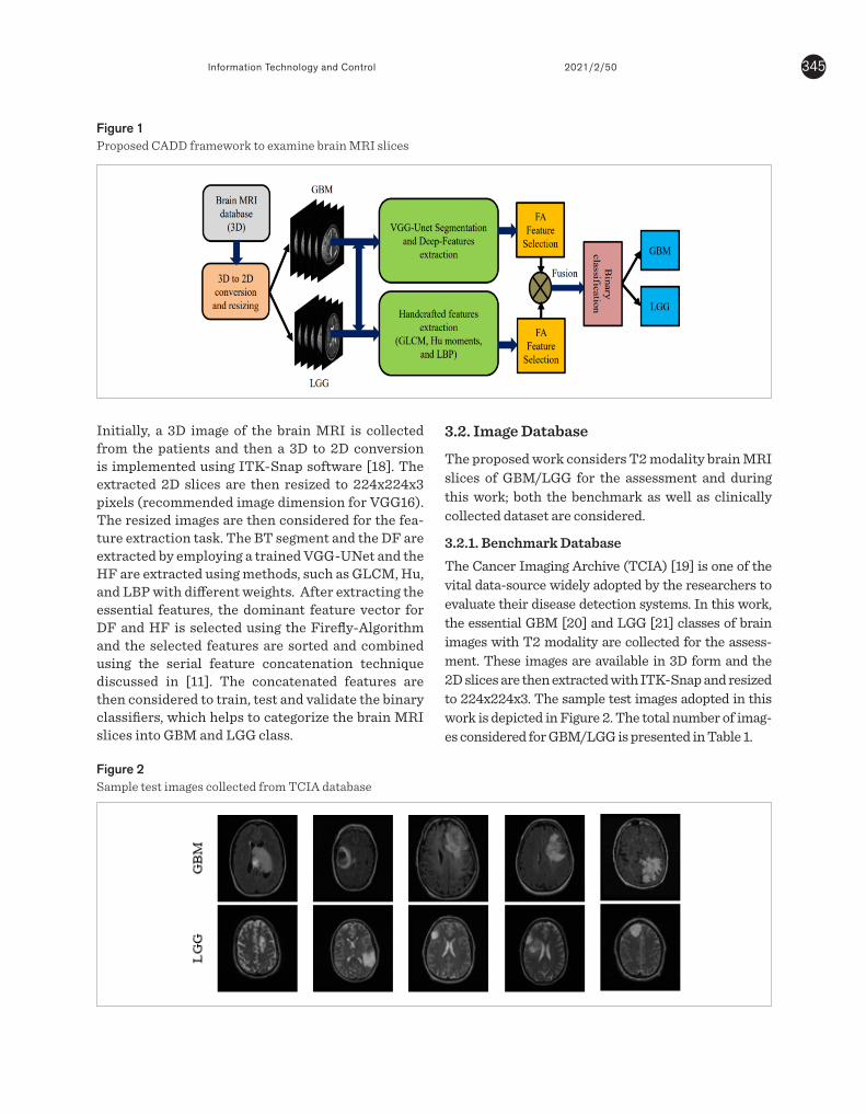
3.1. Disease Detection FrameworkThe CADD unit considered to detect and categorize the BT of brain MRI slices is depicted in Figure 1.
345Information Technology and Control 2021/2/50
Initially, a 3D image of the brain MRI is collected from the patients and then a 3D to 2D conversion is implemented using ITK-Snap software [18]. The extracted 2D slices are then resized to 224x224x3 pixels (recommended image dimension for VGG16). The resized images are then considered for the fea-ture extraction task. The BT segment and the DF are extracted by employing a trained VGG-UNet and the HF are extracted using methods, such as GLCM, Hu, and LBP with different weights. After extracting the essential features, the dominant feature vector for DF and HF is selected using the Firefly-Algorithm and the selected features are sorted and combined using the serial feature concatenation technique discussed in [11]. The concatenated features are then considered to train, test and validate the binary classifiers, which helps to categorize the brain MRI slices into GBM and LGG class.
Figure 1Proposed CADD framework to examine brain MRI slices
Figure 2Sample test images collected from TCIA database
weights. After extracting the essential features, the dominant feature vector for DF and HF is selected using the Firefly-Algorithm and the selected features are sorted and combined using the serial feature concatenation technique discussed in [11]. The concatenated features are then considered to train, test and validate the binary classifiers, which helps to categorize the brain MRI slices into GBM and LGG class.
Figure 1
Proposed CADD framework to examine brain MRI slices
3.2 Image Database
The proposed work considers T2 modality brain MRI slices of GBM/LGG for the assessment and during this work; both the benchmark as well as clinically collected dataset are considered.
3.2.1 Benchmark Database
The Cancer Imaging Archive (TCIA) [19] is one of the vital data-source widely adopted by the researchers to evaluate their disease detection systems. In this work, the essential GBM [20] and LGG [21] classes of brain images with T2 modality are collected for the assessment. These images are available in 3D form and the 2D slices are then extracted with ITK-Snap and resized to 224x224x3. The sample test images adopted in this work is depicted in Figure 2. The total number of images considered for GBM/LGG is presented in Table 1.
Figure 2 Sample test images collected from TCIA database
3.2.2 Clinical Database
The clinical significance of the proposed CADD unit is confirmed by considering the clinically collected real patient’s MRI slices of T2 modality. The earlier works implemented with this dataset can be accessed from [9-11]. All the real patient’s
images are collected based on the approved medical protocol and informed consent is obtained from each patient participated in this study and all this information can be found in [10]. The sample clinical images of GBM/LGG can be found in Figure 3 and number of MRI slices considered in this work is available in Table 1.
Figure 3 Sample T2 modality brain MRI slices of clinical database
Table 1
TCIA and clinical-grade brain MRI slices considered in this study
Image class
Image modality
Dimension Brain MRI Slices
Training Validat
ion TCIA-GBM
T2 224x224x3 560 240
TCIA-LGG
T2 224x224x3 560 240
Clinical-GBM
T2 224x224x3 210 90
Clinical-LGG
T2 224x224x3 210 90
3.3 CNN Segmentation and Feature Extraction
The image segmentation is one of the proven approaches, widely adopted to extract the abnormal section from the test image for further assessment [22, 23]. Automated segmentation is widely adopted compared to semi-automated and traditional procedures and hence, in the proposed work, CNN supported segmentation is implemented to extract the BT segment from the considered brain MRI slices.
3.4 VGG-UNet Implementation
The automated segmentation using UNet is initially proposed in [24]. This scheme included a encoder-decoder section to categorize the image components based on its pixel and for the medical image assessment, a binary classification is employed to extract the abnormal section. In this work, the VGG-
3.2. Image Database
The proposed work considers T2 modality brain MRI slices of GBM/LGG for the assessment and during this work; both the benchmark as well as clinically collected dataset are considered.
3.2.1. Benchmark DatabaseThe Cancer Imaging Archive (TCIA) [19] is one of the vital data-source widely adopted by the researchers to evaluate their disease detection systems. In this work, the essential GBM [20] and LGG [21] classes of brain images with T2 modality are collected for the assess-ment. These images are available in 3D form and the 2D slices are then extracted with ITK-Snap and resized to 224x224x3. The sample test images adopted in this work is depicted in Figure 2. The total number of imag-es considered for GBM/LGG is presented in Table 1.
weights. After extracting the essential features, the dominant feature vector for DF and HF is selected using the Firefly-Algorithm and the selected features are sorted and combined using the serial feature concatenation technique discussed in [11]. The concatenated features are then considered to train, test and validate the binary classifiers, which helps to categorize the brain MRI slices into GBM and LGG class.
Figure 1
Proposed CADD framework to examine brain MRI slices
3.2 Image Database
The proposed work considers T2 modality brain MRI slices of GBM/LGG for the assessment and during this work; both the benchmark as well as clinically collected dataset are considered.
3.2.1 Benchmark Database
The Cancer Imaging Archive (TCIA) [19] is one of the vital data-source widely adopted by the researchers to evaluate their disease detection systems. In this work, the essential GBM [20] and LGG [21] classes of brain images with T2 modality are collected for the assessment. These images are available in 3D form and the 2D slices are then extracted with ITK-Snap and resized to 224x224x3. The sample test images adopted in this work is depicted in Figure 2. The total number of images considered for GBM/LGG is presented in Table 1.
Figure 2 Sample test images collected from TCIA database
3.2.2 Clinical Database
The clinical significance of the proposed CADD unit is confirmed by considering the clinically collected real patient’s MRI slices of T2 modality. The earlier works implemented with this dataset can be accessed from [9-11]. All the real patient’s
images are collected based on the approved medical protocol and informed consent is obtained from each patient participated in this study and all this information can be found in [10]. The sample clinical images of GBM/LGG can be found in Figure 3 and number of MRI slices considered in this work is available in Table 1.
Figure 3 Sample T2 modality brain MRI slices of clinical database
Table 1
TCIA and clinical-grade brain MRI slices considered in this study
Image class
Image modality
Dimension Brain MRI Slices
Training Validat
ion TCIA-GBM
T2 224x224x3 560 240
TCIA-LGG
T2 224x224x3 560 240
Clinical-GBM
T2 224x224x3 210 90
Clinical-LGG
T2 224x224x3 210 90
3.3 CNN Segmentation and Feature Extraction
The image segmentation is one of the proven approaches, widely adopted to extract the abnormal section from the test image for further assessment [22, 23]. Automated segmentation is widely adopted compared to semi-automated and traditional procedures and hence, in the proposed work, CNN supported segmentation is implemented to extract the BT segment from the considered brain MRI slices.
3.4 VGG-UNet Implementation
The automated segmentation using UNet is initially proposed in [24]. This scheme included a encoder-decoder section to categorize the image components based on its pixel and for the medical image assessment, a binary classification is employed to extract the abnormal section. In this work, the VGG-

Information Technology and Control 2021/2/50346
Figure 3Sample T2 modality brain MRI slices of clinical database
Table 1TCIA and clinical-grade brain MRI slices considered in this study
3.2.2. Clinical DatabaseThe clinical significance of the proposed CADD unit is confirmed by considering the clinically collected real patient’s MRI slices of T2 modality. The earlier works implemented with this dataset can be accessed from [9-11]. All the real patient’s images are collected based on the approved medical protocol and informed consent is obtained from each patient participated in this study and all this information can be found in [10]. The sample clinical images of GBM/LGG can be found in Figure 3 and number of MRI slices consid-ered in this work is available in Table 1.
3.3. CNN Segmentation and Feature ExtractionThe image segmentation is one of the proven ap-proaches, widely adopted to extract the abnormal section from the test image for further assessment
Image class Imagemodality Dimension
Brain MRI Slices
Training Validation
TCIA-GBM T2 224x224x3 560 240
TCIA-LGG T2 224x224x3 560 240
Clinical-GBM T2 224x224x3 210 90
Clinical-LGG T2 224x224x3 210 90
weights. After extracting the essential features, the dominant feature vector for DF and HF is selected using the Firefly-Algorithm and the selected features are sorted and combined using the serial feature concatenation technique discussed in [11]. The concatenated features are then considered to train, test and validate the binary classifiers, which helps to categorize the brain MRI slices into GBM and LGG class.
Figure 1
Proposed CADD framework to examine brain MRI slices
3.2 Image Database
The proposed work considers T2 modality brain MRI slices of GBM/LGG for the assessment and during this work; both the benchmark as well as clinically collected dataset are considered.
3.2.1 Benchmark Database
The Cancer Imaging Archive (TCIA) [19] is one of the vital data-source widely adopted by the researchers to evaluate their disease detection systems. In this work, the essential GBM [20] and LGG [21] classes of brain images with T2 modality are collected for the assessment. These images are available in 3D form and the 2D slices are then extracted with ITK-Snap and resized to 224x224x3. The sample test images adopted in this work is depicted in Figure 2. The total number of images considered for GBM/LGG is presented in Table 1.
Figure 2 Sample test images collected from TCIA database
3.2.2 Clinical Database
The clinical significance of the proposed CADD unit is confirmed by considering the clinically collected real patient’s MRI slices of T2 modality. The earlier works implemented with this dataset can be accessed from [9-11]. All the real patient’s
images are collected based on the approved medical protocol and informed consent is obtained from each patient participated in this study and all this information can be found in [10]. The sample clinical images of GBM/LGG can be found in Figure 3 and number of MRI slices considered in this work is available in Table 1.
Figure 3 Sample T2 modality brain MRI slices of clinical database
Table 1
TCIA and clinical-grade brain MRI slices considered in this study
Image class
Image modality
Dimension Brain MRI Slices
Training Validat
ion TCIA-GBM
T2 224x224x3 560 240
TCIA-LGG
T2 224x224x3 560 240
Clinical-GBM
T2 224x224x3 210 90
Clinical-LGG
T2 224x224x3 210 90
3.3 CNN Segmentation and Feature Extraction
The image segmentation is one of the proven approaches, widely adopted to extract the abnormal section from the test image for further assessment [22, 23]. Automated segmentation is widely adopted compared to semi-automated and traditional procedures and hence, in the proposed work, CNN supported segmentation is implemented to extract the BT segment from the considered brain MRI slices.
3.4 VGG-UNet Implementation
The automated segmentation using UNet is initially proposed in [24]. This scheme included a encoder-decoder section to categorize the image components based on its pixel and for the medical image assessment, a binary classification is employed to extract the abnormal section. In this work, the VGG-
[22, 23]. Automated segmentation is widely adopted compared to semi-automated and traditional proce-dures and hence, in the proposed work, CNN support-ed segmentation is implemented to extract the BT segment from the considered brain MRI slices.
3.4. VGG-UNet Implementation The automated segmentation using UNet is initially proposed in [24]. This scheme included a encoder-de-coder section to categorize the image components based on its pixel and for the medical image assess-ment, a binary classification is employed to extract the abnormal section. In this work, the VGG-UNet scheme depicted in Figure 4 is employed to extract the BT with better accuracy. The essential informa-tion on VGG-UNet can be accessed from [25-27]. The initial part (encoder) of VGG-UNet consists of the
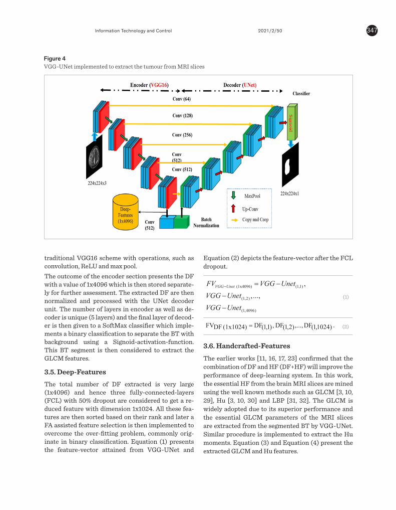
347Information Technology and Control 2021/2/50
traditional VGG16 scheme with operations, such as convolution, ReLU and max pool. The outcome of the encoder section presents the DF with a value of 1x4096 which is then stored separate-ly for further assessment. The extracted DF are then normalized and processed with the UNet decoder unit. The number of layers in encoder as well as de-coder is unique (5 layers) and the final layer of decod-er is then given to a SoftMax classifier which imple-ments a binary classification to separate the BT with background using a Signoid-activation-function. This BT segment is then considered to extract the GLCM features.
3.5. Deep-Features The total number of DF extracted is very large (1x4096) and hence three fully-connected-layers (FCL) with 50% dropout are considered to get a re-duced feature with dimension 1x1024. All these fea-tures are then sorted based on their rank and later a FA assisted feature selection is then implemented to overcome the over-fitting problem, commonly orig-inate in binary classification. Equation (1) presents the feature-vector attained from VGG-UNet and
Figure 4VGG-UNet implemented to extract the tumour from MRI slices
UNet scheme depicted in Figure 4 is employed to extract the BT with better accuracy. The essential information on VGG-UNet can be accessed from [25-27]. The initial part (encoder) of VGG-UNet consists of the traditional VGG16 scheme with operations, such as convolution, ReLU and max pool.
The outcome of the encoder section presents the DF with a value of 1x4096 which is then stored separately for further assessment. The extracted DF are then normalized and processed with the UNet decoder unit. The number of layers in encoder as well as decoder is unique (5 layers) and the final layer of decoder is then given to a SoftMax classifier which implements a binary classification to separate the BT with background using a Signoid-activation-function. This BT segment is then considered to extract the GLCM features.
Figure 4
VGG-UNet implemented to extract the tumour from MRI slices
3.5 Deep-Features
The total number of DF extracted is very large (1x4096) and hence three fully-connected-layers (FCL) with 50% dropout are considered to get a reduced feature with dimension 1x1024. All these features are then sorted based on their rank and later a FA assisted feature selection is then implemented to overcome the over-fitting problem, commonly originate in binary classification. Equation (1) presents the feature-vector attained from VGG-UNet and Equation (2) depicts the feature-vector after the FCL dropout.
(1x4096) (1,1)
(1,2)
(1,4096)
,,...,
VGG UnetFV VGG UnetVGG UnetVGG Unet
− = −
−
−
(1)
)1024,1(DF,...,)2,1(DF ,)1,1(DF(1x1024) FDFV = . (2)
3.6 Handcrafted-Features
The earlier works [11, 16, 17, 23] confirmed that the combination of DF and HF (DF+HF) will improve the performance of deep-learning system. In this work, the essential HF from the brain MRI slices are mined using the well known methods such as GLCM [3, 10, 29], Hu [3, 10, 30] and LBP [31, 32]. The GLCM is widely adopted due to its superior performance and the essential GLCM parameters of the MRI slices are extracted from the segmented BT by VGG-UNet. Similar procedure is implemented to extract the Hu moments. Equation (3) and Equation (4) present the extracted GLCM and Hu features.
LCM (1x25) (1,1) (1,2)
(1,25)
1 , ,...,GHF GLCM GLCMGLCM
=(3)
)7,1(Hu,...,)2,1(Hu,)1,1(Hu(1x7)u H2HF = . (4)
The LBP provides the important information regarding the gray-scale picture under assessment and the LBP with different weight discussed in [32] is adopted to extract the pixel information of MRI slices with GBM/LGG. In this work, the weights, such as W=1, 2, 3, and 4 are considered to enhance the image and from each image, 1x59 number of features are extracted. The LBP features considered in this work are depicted in Equation (5):
(1x236) (1,59) (1,59)
(1,59) (1,59)
3 1 23 4
LBPHF LBP LBPLBP LBP
= +
+ + . (5)
The total number of HF collected with GLCM, Hu and LBP is shown in Equation (6);
(1 268) LCM (1x25) u (1x7)
(1x236)
1 23
x G H
LBP
HF HF HFHF
= +
+ . (6)
3.6 Firefly-Algorithm Based Feature Selection and Serial Fusion
The feature reduction process plays a vital role during in ML and DL based classification and to avoid the over-fitting problem, it is necessary to identify the dominant features using an appropriate approach. The feature reduction can be implemented using traditional statistical approaches (Student’s t-test) [3, 12] and heuristic algorithm assisted techniques [17, 22]. In this work, the feature reduction for DF and HF are implemented using the FA algorithm and the reduced features are then serially combined as
Equation (2) depicts the feature-vector after the FCL dropout.
UNet scheme depicted in Figure 4 is employed to extract the BT with better accuracy. The essential information on VGG-UNet can be accessed from [25-27]. The initial part (encoder) of VGG-UNet consists of the traditional VGG16 scheme with operations, such as convolution, ReLU and max pool.
The outcome of the encoder section presents the DF with a value of 1x4096 which is then stored separately for further assessment. The extracted DF are then normalized and processed with the UNet decoder unit. The number of layers in encoder as well as decoder is unique (5 layers) and the final layer of decoder is then given to a SoftMax classifier which implements a binary classification to separate the BT with background using a Signoid-activation-function. This BT segment is then considered to extract the GLCM features.
Figure 4
VGG-UNet implemented to extract the tumour from MRI slices
3.5 Deep-Features
The total number of DF extracted is very large (1x4096) and hence three fully-connected-layers (FCL) with 50% dropout are considered to get a reduced feature with dimension 1x1024. All these features are then sorted based on their rank and later a FA assisted feature selection is then implemented to overcome the over-fitting problem, commonly originate in binary classification. Equation (1) presents the feature-vector attained from VGG-UNet and Equation (2) depicts the feature-vector after the FCL dropout.
(1x4096) (1,1)
(1,2)
(1,4096)
,,...,
VGG UnetFV VGG UnetVGG UnetVGG Unet
− = −
−
−
(1)
)1024,1(DF,...,)2,1(DF ,)1,1(DF(1x1024) FDFV = . (2)
3.6 Handcrafted-Features
The earlier works [11, 16, 17, 23] confirmed that the combination of DF and HF (DF+HF) will improve the performance of deep-learning system. In this work, the essential HF from the brain MRI slices are mined using the well known methods such as GLCM [3, 10, 29], Hu [3, 10, 30] and LBP [31, 32]. The GLCM is widely adopted due to its superior performance and the essential GLCM parameters of the MRI slices are extracted from the segmented BT by VGG-UNet. Similar procedure is implemented to extract the Hu moments. Equation (3) and Equation (4) present the extracted GLCM and Hu features.
LCM (1x25) (1,1) (1,2)
(1,25)
1 , ,...,GHF GLCM GLCMGLCM
=(3)
)7,1(Hu,...,)2,1(Hu,)1,1(Hu(1x7)u H2HF = . (4)
The LBP provides the important information regarding the gray-scale picture under assessment and the LBP with different weight discussed in [32] is adopted to extract the pixel information of MRI slices with GBM/LGG. In this work, the weights, such as W=1, 2, 3, and 4 are considered to enhance the image and from each image, 1x59 number of features are extracted. The LBP features considered in this work are depicted in Equation (5):
(1x236) (1,59) (1,59)
(1,59) (1,59)
3 1 23 4
LBPHF LBP LBPLBP LBP
= +
+ + . (5)
The total number of HF collected with GLCM, Hu and LBP is shown in Equation (6);
(1 268) LCM (1x25) u (1x7)
(1x236)
1 23
x G H
LBP
HF HF HFHF
= +
+ . (6)
3.6 Firefly-Algorithm Based Feature Selection and Serial Fusion
The feature reduction process plays a vital role during in ML and DL based classification and to avoid the over-fitting problem, it is necessary to identify the dominant features using an appropriate approach. The feature reduction can be implemented using traditional statistical approaches (Student’s t-test) [3, 12] and heuristic algorithm assisted techniques [17, 22]. In this work, the feature reduction for DF and HF are implemented using the FA algorithm and the reduced features are then serially combined as
(1)
UNet scheme depicted in Figure 4 is employed to extract the BT with better accuracy. The essential information on VGG-UNet can be accessed from [25-27]. The initial part (encoder) of VGG-UNet consists of the traditional VGG16 scheme with operations, such as convolution, ReLU and max pool.
The outcome of the encoder section presents the DF with a value of 1x4096 which is then stored separately for further assessment. The extracted DF are then normalized and processed with the UNet decoder unit. The number of layers in encoder as well as decoder is unique (5 layers) and the final layer of decoder is then given to a SoftMax classifier which implements a binary classification to separate the BT with background using a Signoid-activation-function. This BT segment is then considered to extract the GLCM features.
Figure 4
VGG-UNet implemented to extract the tumour from MRI slices
3.5 Deep-Features
The total number of DF extracted is very large (1x4096) and hence three fully-connected-layers (FCL) with 50% dropout are considered to get a reduced feature with dimension 1x1024. All these features are then sorted based on their rank and later a FA assisted feature selection is then implemented to overcome the over-fitting problem, commonly originate in binary classification. Equation (1) presents the feature-vector attained from VGG-UNet and Equation (2) depicts the feature-vector after the FCL dropout.
(1x4096) (1,1)
(1,2)
(1,4096)
,,...,
VGG UnetFV VGG UnetVGG UnetVGG Unet
− = −
−
−
(1)
)1024,1(DF,...,)2,1(DF ,)1,1(DF(1x1024) FDFV = . (2)
3.6 Handcrafted-Features
The earlier works [11, 16, 17, 23] confirmed that the combination of DF and HF (DF+HF) will improve the performance of deep-learning system. In this work, the essential HF from the brain MRI slices are mined using the well known methods such as GLCM [3, 10, 29], Hu [3, 10, 30] and LBP [31, 32]. The GLCM is widely adopted due to its superior performance and the essential GLCM parameters of the MRI slices are extracted from the segmented BT by VGG-UNet. Similar procedure is implemented to extract the Hu moments. Equation (3) and Equation (4) present the extracted GLCM and Hu features.
LCM (1x25) (1,1) (1,2)
(1,25)
1 , ,...,GHF GLCM GLCMGLCM
=(3)
)7,1(Hu,...,)2,1(Hu,)1,1(Hu(1x7)u H2HF = . (4)
The LBP provides the important information regarding the gray-scale picture under assessment and the LBP with different weight discussed in [32] is adopted to extract the pixel information of MRI slices with GBM/LGG. In this work, the weights, such as W=1, 2, 3, and 4 are considered to enhance the image and from each image, 1x59 number of features are extracted. The LBP features considered in this work are depicted in Equation (5):
(1x236) (1,59) (1,59)
(1,59) (1,59)
3 1 23 4
LBPHF LBP LBPLBP LBP
= +
+ + . (5)
The total number of HF collected with GLCM, Hu and LBP is shown in Equation (6);
(1 268) LCM (1x25) u (1x7)
(1x236)
1 23
x G H
LBP
HF HF HFHF
= +
+ . (6)
3.6 Firefly-Algorithm Based Feature Selection and Serial Fusion
The feature reduction process plays a vital role during in ML and DL based classification and to avoid the over-fitting problem, it is necessary to identify the dominant features using an appropriate approach. The feature reduction can be implemented using traditional statistical approaches (Student’s t-test) [3, 12] and heuristic algorithm assisted techniques [17, 22]. In this work, the feature reduction for DF and HF are implemented using the FA algorithm and the reduced features are then serially combined as
(2)
3.6. Handcrafted-Features
The earlier works [11, 16, 17, 23] confirmed that the combination of DF and HF (DF+HF) will improve the performance of deep-learning system. In this work, the essential HF from the brain MRI slices are mined using the well known methods such as GLCM [3, 10, 29], Hu [3, 10, 30] and LBP [31, 32]. The GLCM is widely adopted due to its superior performance and the essential GLCM parameters of the MRI slices are extracted from the segmented BT by VGG-UNet. Similar procedure is implemented to extract the Hu moments. Equation (3) and Equation (4) present the extracted GLCM and Hu features.
Information Technology and Control 2021/2/50348
UNet scheme depicted in Figure 4 is employed to extract the BT with better accuracy. The essential information on VGG-UNet can be accessed from [25-27]. The initial part (encoder) of VGG-UNet consists of the traditional VGG16 scheme with operations, such as convolution, ReLU and max pool.
The outcome of the encoder section presents the DF with a value of 1x4096 which is then stored separately for further assessment. The extracted DF are then normalized and processed with the UNet decoder unit. The number of layers in encoder as well as decoder is unique (5 layers) and the final layer of decoder is then given to a SoftMax classifier which implements a binary classification to separate the BT with background using a Signoid-activation-function. This BT segment is then considered to extract the GLCM features.
Figure 4
VGG-UNet implemented to extract the tumour from MRI slices
3.5 Deep-Features
The total number of DF extracted is very large (1x4096) and hence three fully-connected-layers (FCL) with 50% dropout are considered to get a reduced feature with dimension 1x1024. All these features are then sorted based on their rank and later a FA assisted feature selection is then implemented to overcome the over-fitting problem, commonly originate in binary classification. Equation (1) presents the feature-vector attained from VGG-UNet and Equation (2) depicts the feature-vector after the FCL dropout.
(1x4096) (1,1)
(1,2)
(1,4096)
,,...,
VGG UnetFV VGG UnetVGG UnetVGG Unet
− = −
−
−
(1)
)1024,1(DF,...,)2,1(DF ,)1,1(DF(1x1024) FDFV = . (2)
3.6 Handcrafted-Features
The earlier works [11, 16, 17, 23] confirmed that the combination of DF and HF (DF+HF) will improve the performance of deep-learning system. In this work, the essential HF from the brain MRI slices are mined using the well known methods such as GLCM [3, 10, 29], Hu [3, 10, 30] and LBP [31, 32]. The GLCM is widely adopted due to its superior performance and the essential GLCM parameters of the MRI slices are extracted from the segmented BT by VGG-UNet. Similar procedure is implemented to extract the Hu moments. Equation (3) and Equation (4) present the extracted GLCM and Hu features.
LCM (1x25) (1,1) (1,2)
(1,25)
1 , ,...,GHF GLCM GLCMGLCM
=(3)
)7,1(Hu,...,)2,1(Hu,)1,1(Hu(1x7)u H2HF = . (4)
The LBP provides the important information regarding the gray-scale picture under assessment and the LBP with different weight discussed in [32] is adopted to extract the pixel information of MRI slices with GBM/LGG. In this work, the weights, such as W=1, 2, 3, and 4 are considered to enhance the image and from each image, 1x59 number of features are extracted. The LBP features considered in this work are depicted in Equation (5):
(1x236) (1,59) (1,59)
(1,59) (1,59)
3 1 23 4
LBPHF LBP LBPLBP LBP
= +
+ + . (5)
The total number of HF collected with GLCM, Hu and LBP is shown in Equation (6);
(1 268) LCM (1x25) u (1x7)
(1x236)
1 23
x G H
LBP
HF HF HFHF
= +
+ . (6)
3.6 Firefly-Algorithm Based Feature Selection and Serial Fusion
The feature reduction process plays a vital role during in ML and DL based classification and to avoid the over-fitting problem, it is necessary to identify the dominant features using an appropriate approach. The feature reduction can be implemented using traditional statistical approaches (Student’s t-test) [3, 12] and heuristic algorithm assisted techniques [17, 22]. In this work, the feature reduction for DF and HF are implemented using the FA algorithm and the reduced features are then serially combined as
(3)
UNet scheme depicted in Figure 4 is employed to extract the BT with better accuracy. The essential information on VGG-UNet can be accessed from [25-27]. The initial part (encoder) of VGG-UNet consists of the traditional VGG16 scheme with operations, such as convolution, ReLU and max pool.
The outcome of the encoder section presents the DF with a value of 1x4096 which is then stored separately for further assessment. The extracted DF are then normalized and processed with the UNet decoder unit. The number of layers in encoder as well as decoder is unique (5 layers) and the final layer of decoder is then given to a SoftMax classifier which implements a binary classification to separate the BT with background using a Signoid-activation-function. This BT segment is then considered to extract the GLCM features.
Figure 4
VGG-UNet implemented to extract the tumour from MRI slices
3.5 Deep-Features
The total number of DF extracted is very large (1x4096) and hence three fully-connected-layers (FCL) with 50% dropout are considered to get a reduced feature with dimension 1x1024. All these features are then sorted based on their rank and later a FA assisted feature selection is then implemented to overcome the over-fitting problem, commonly originate in binary classification. Equation (1) presents the feature-vector attained from VGG-UNet and Equation (2) depicts the feature-vector after the FCL dropout.
(1x4096) (1,1)
(1,2)
(1,4096)
,,...,
VGG UnetFV VGG UnetVGG UnetVGG Unet
− = −
−
−
(1)
)1024,1(DF,...,)2,1(DF ,)1,1(DF(1x1024) FDFV = . (2)
3.6 Handcrafted-Features
The earlier works [11, 16, 17, 23] confirmed that the combination of DF and HF (DF+HF) will improve the performance of deep-learning system. In this work, the essential HF from the brain MRI slices are mined using the well known methods such as GLCM [3, 10, 29], Hu [3, 10, 30] and LBP [31, 32]. The GLCM is widely adopted due to its superior performance and the essential GLCM parameters of the MRI slices are extracted from the segmented BT by VGG-UNet. Similar procedure is implemented to extract the Hu moments. Equation (3) and Equation (4) present the extracted GLCM and Hu features.
LCM (1x25) (1,1) (1,2)
(1,25)
1 , ,...,GHF GLCM GLCMGLCM
=(3)
)7,1(Hu,...,)2,1(Hu,)1,1(Hu(1x7)u H2HF = . (4)
The LBP provides the important information regarding the gray-scale picture under assessment and the LBP with different weight discussed in [32] is adopted to extract the pixel information of MRI slices with GBM/LGG. In this work, the weights, such as W=1, 2, 3, and 4 are considered to enhance the image and from each image, 1x59 number of features are extracted. The LBP features considered in this work are depicted in Equation (5):
(1x236) (1,59) (1,59)
(1,59) (1,59)
3 1 23 4
LBPHF LBP LBPLBP LBP
= +
+ + . (5)
The total number of HF collected with GLCM, Hu and LBP is shown in Equation (6);
(1 268) LCM (1x25) u (1x7)
(1x236)
1 23
x G H
LBP
HF HF HFHF
= +
+ . (6)
3.6 Firefly-Algorithm Based Feature Selection and Serial Fusion
The feature reduction process plays a vital role during in ML and DL based classification and to avoid the over-fitting problem, it is necessary to identify the dominant features using an appropriate approach. The feature reduction can be implemented using traditional statistical approaches (Student’s t-test) [3, 12] and heuristic algorithm assisted techniques [17, 22]. In this work, the feature reduction for DF and HF are implemented using the FA algorithm and the reduced features are then serially combined as
(4)
The LBP provides the important information regard-ing the gray-scale picture under assessment and the LBP with different weight discussed in [32] is adopt-ed to extract the pixel information of MRI slices with GBM/LGG. In this work, the weights, such as W=1, 2, 3, and 4 are considered to enhance the image and from each image, 1x59 number of features are extracted. The LBP features considered in this work are depict-ed in Equation (5):
UNet scheme depicted in Figure 4 is employed to extract the BT with better accuracy. The essential information on VGG-UNet can be accessed from [25-27]. The initial part (encoder) of VGG-UNet consists of the traditional VGG16 scheme with operations, such as convolution, ReLU and max pool.
The outcome of the encoder section presents the DF with a value of 1x4096 which is then stored separately for further assessment. The extracted DF are then normalized and processed with the UNet decoder unit. The number of layers in encoder as well as decoder is unique (5 layers) and the final layer of decoder is then given to a SoftMax classifier which implements a binary classification to separate the BT with background using a Signoid-activation-function. This BT segment is then considered to extract the GLCM features.
Figure 4
VGG-UNet implemented to extract the tumour from MRI slices
3.5 Deep-Features
The total number of DF extracted is very large (1x4096) and hence three fully-connected-layers (FCL) with 50% dropout are considered to get a reduced feature with dimension 1x1024. All these features are then sorted based on their rank and later a FA assisted feature selection is then implemented to overcome the over-fitting problem, commonly originate in binary classification. Equation (1) presents the feature-vector attained from VGG-UNet and Equation (2) depicts the feature-vector after the FCL dropout.
(1x4096) (1,1)
(1,2)
(1,4096)
,,...,
VGG UnetFV VGG UnetVGG UnetVGG Unet
− = −
−
−
(1)
)1024,1(DF,...,)2,1(DF ,)1,1(DF(1x1024) FDFV = . (2)
3.6 Handcrafted-Features
The earlier works [11, 16, 17, 23] confirmed that the combination of DF and HF (DF+HF) will improve the performance of deep-learning system. In this work, the essential HF from the brain MRI slices are mined using the well known methods such as GLCM [3, 10, 29], Hu [3, 10, 30] and LBP [31, 32]. The GLCM is widely adopted due to its superior performance and the essential GLCM parameters of the MRI slices are extracted from the segmented BT by VGG-UNet. Similar procedure is implemented to extract the Hu moments. Equation (3) and Equation (4) present the extracted GLCM and Hu features.
LCM (1x25) (1,1) (1,2)
(1,25)
1 , ,...,GHF GLCM GLCMGLCM
=(3)
)7,1(Hu,...,)2,1(Hu,)1,1(Hu(1x7)u H2HF = . (4)
The LBP provides the important information regarding the gray-scale picture under assessment and the LBP with different weight discussed in [32] is adopted to extract the pixel information of MRI slices with GBM/LGG. In this work, the weights, such as W=1, 2, 3, and 4 are considered to enhance the image and from each image, 1x59 number of features are extracted. The LBP features considered in this work are depicted in Equation (5):
(1x236) (1,59) (1,59)
(1,59) (1,59)
3 1 23 4
LBPHF LBP LBPLBP LBP
= +
+ + .
The total number of HF collected with GLCM, Hu and LBP is shown in
Equation (6); (1 268) LCM (1x25) u (1x7)
(1x236)
1 23
x G H
LBP
HF HF HFHF
= +
+ . (6)
3.6 Firefly-Algorithm Based Feature Selection and Serial Fusion
The feature reduction process plays a vital role during in ML and DL based classification and to avoid the over-fitting problem, it is necessary to identify the dominant features using an appropriate approach. The feature reduction can be implemented using traditional statistical approaches (Student’s t-test) [3, 12] and heuristic algorithm assisted techniques [17, 22]. In this work, the feature reduction for DF and HF are implemented using the FA algorithm and the reduced features are then serially combined as
(5)
The total number of HF collected with GLCM, Hu and LBP is shown in Equation (6);
UNet scheme depicted in Figure 4 is employed to extract the BT with better accuracy. The essential information on VGG-UNet can be accessed from [25-27]. The initial part (encoder) of VGG-UNet consists of the traditional VGG16 scheme with operations, such as convolution, ReLU and max pool.
The outcome of the encoder section presents the DF with a value of 1x4096 which is then stored separately for further assessment. The extracted DF are then normalized and processed with the UNet decoder unit. The number of layers in encoder as well as decoder is unique (5 layers) and the final layer of decoder is then given to a SoftMax classifier which implements a binary classification to separate the BT with background using a Signoid-activation-function. This BT segment is then considered to extract the GLCM features.
Figure 4
VGG-UNet implemented to extract the tumour from MRI slices
3.5 Deep-Features
The total number of DF extracted is very large (1x4096) and hence three fully-connected-layers (FCL) with 50% dropout are considered to get a reduced feature with dimension 1x1024. All these features are then sorted based on their rank and later a FA assisted feature selection is then implemented to overcome the over-fitting probleclassification. Equation vector attained from VGG-UNet and Equation depicts the feature-
(1x4096) (1,1)
(1,2)
(1,4096)
,,...,
VGG UnetFV VGG UnetVGG UnetVGG Unet
− = −
−
−
)1024,1(DF,...,)2,1(DF ,)1,1(DF(1x1024) FDFV = . (2)
3.6 Handcrafted-Features
The earlier works [11, 16, 17, 23] confirmed that the combination of DF and HF (DF+HF) will improve the performance of deep-learning system. In this work, the essential HF from the brain MRI slices are mined using the well known methods such as GLCM [3, 10, 29], Hu [3, 10, 30] and LBP [31, 32]. The GLCM is widely adopted due to its superior performance and the essential GLCM parameters of the MRI slices are extracted from the segmented BT by VGG-UNet. Similar procedure is implemented to extract the Hu moments. Equation (3) and Equation (4) present the extracted GLCM and Hu features.
LCM (1x25) (1,1) (1,2)
(1,25)
1 , ,...,GHF GLCM GLCMGLCM
=(3)
)7,1(Hu,...,)2,1(Hu,)1,1(Hu(1x7)u H2HF = . (4)
The LBP provides the important information regarding the gray-scale picture under assessment and the LBP with different weight discussed in [32] is adopted to extract the pixel information of MRI slices with GBM/LGG. In this work, the weights, such as W=1, 2, 3, and 4 are considered to enhance the image and from each image, 1x59 number of features are extracted. The LBP features considered in this work are depicted in Equation (5):
(1x236) (1,59) (1,59)
(1,59) (1,59)
3 1 23 4
LBPHF LBP LBPLBP LBP
= +
+ + . (5)
The total number of HF collected with GLCM, Hu and LBP is shown in Equation (6);
(1 268) LCM (1x25) u (1x7)
(1x236)
1 23
x G H
LBP
HF HF HFHF
= +
+ . (6)
3.6 Firefly-Algorithm Based Feature Selection and Serial Fusion
reduction for DF and HF are implemented using the FA algorithm and the reduced features are then serially combined as
(6)
3.6. Firefly-Algorithm Based Feature Selection and Serial FusionThe feature reduction process plays a vital role during in ML and DL based classification and to avoid the over-fitting problem, it is necessary to identify the dominant features using an appropriate approach. The feature reduction can be implemented using tradition-al statistical approaches (Student’s t-test) [3, 12] and heuristic algorithm assisted techniques [17, 22]. In this work, the feature reduction for DF and HF are imple-mented using the FA algorithm and the reduced fea-tures are then serially combined as discussed in [33]. The FA feature selection is implemented as follows;Let us consider there exist feature vectors
discussed in [33].
The FA feature selection is implemented as follows;
Let us consider there exist feature vectors GBMFV and; let this vector is with a value of { }N1,0LGGFV,GBMFV ∈ . The FA then performs a feature wise assessment and computes the Hamming-Distance (HD) as in Equation (7):.
∑=
−=N
1aLGGaFVGBMaFV)LGGFV,GBMFV( HD , (7)
where N=1024 in DF and N=268 in HF
The difference in values between features is expressed as in Equation (8);
1iff ( , ) ( ).
N
GBM LGG GBMa LGGaa
D FV FV FV FV=
= −∑ (8)
The fitness function then assigned as in Equation (9):
max
1
( , )GBM LGGN
GBMa LGGaa
Fitnessvalue HD FV FV
FV FV=
= =
−∑
(9)
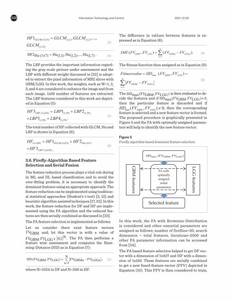
The )LGGFV,GBMFV( maxHD is then evaluated to decide the features and if 0)LGGFV,GBMFV( maxHD ≈ , then the particular feature is discarded and if max ( , ) 0,GBM LGGHD FV FV ≠ then the corresponding feature is selected and a new feature vector is formed. The proposed procedure is graphically presented in Figure 5 and the FA with optimally assigned parameters will help to identify the new feature vector.
Figure 5
Firefly algorithm based dominant feature selection
In this work, the FA with Brownian-Distribution is considered and other essential parameters are assigned as follows; number of fireflies=30, search dimension = total features, iterations=2500 and
other FA parameter information can be accessed from [34].
The FA based feature selection helped to get DF vector with a dimension of 1x427 and HF with a dimension of 1x193. These features are serially combined to get a new fused-feature-vector (FFV) depicted in Equation (10). This FFV is then considered to train, test and validate the binary classifiers considered in the developed CADD unit.
)193x1(HF)427x1(DF)620x1(FFV += . (10)
3.7 Classifier Implementation and Performance Validation
The performance of the medical data assessment using the developed CADD depends on the employed classifiers. Binary classification is implemented in the proposed work to classify the MRI slices into GBM/LGG class for benchmark as well as clinical data. To achieve this task, the classifiers existing in the literature, such as SoftMax, SVM with various kernels (Linear, RBF, and Cubic) [3, 12, 33, 35-37], DA (Linear, and Quadratic) [12,33] and KNN (Fine, and Cubic) [12,33] are employed to accomplish the task. The earlier research also presents the similar medical image assessment tasks which implemented classifiers [38-41].
The performance of the classifier is then assessed by recording the confusion-matrix values, such as true-positive (TP), true-negative (TN), false-positive (FP), false-negative (FN), accuracy (ACC), precision (PRE), sensitivity (SEN), specificity (SPE) and negative predictive value (NPV) [3, 11]. Based on these values, the performance of proposed CADD with a chosen binary classifier is confirmed.
4. Experimental Results This section presents the experimental outcome attained with the proposed work. The experimental investigation is implemented using a workstation with Intel I5 2.5GHz processor with 16GB RAM and 2GB VRAM equipped with MATLAB®.
Initially, the essential number of MRI slices is extracted from benchmark as well as the clinical dataset as discussed in Table 1 and every image is then resized into 3x224x224 pixels to implement the selected CNN
FA with optimally assigned
initial parameters
GBM
features
)FV,FV( HD LGGGBMmax
LGG
features
Selected feature
and; let this vector is with a value of
discussed in [33].
The FA feature selection is implemented as follows;
Let us consider there exist feature vectors GBMFV and; let this vector is with a value of { }N1,0LGGFV,GBMFV ∈ . The FA then performs a feature wise assessment and computes the Hamming-Distance (HD) as in Equation (7):.
∑=
−=N
1aLGGaFVGBMaFV)LGGFV,GBMFV( HD , (7)
where N=1024 in DF and N=268 in HF
The difference in values between features is expressed as in Equation (8);
1iff ( , ) ( ).
N
GBM LGG GBMa LGGaa
D FV FV FV FV=
= −∑ (8)
The fitness function then assigned as in Equation (9):
max
1
( , )GBM LGGN
GBMa LGGaa
Fitnessvalue HD FV FV
FV FV=
= =
−∑
(9)
The )LGGFV,GBMFV( maxHD is then evaluated to decide the features and if 0)LGGFV,GBMFV( maxHD ≈ , then the particular feature is discarded and if max ( , ) 0,GBM LGGHD FV FV ≠ then the corresponding feature is selected and a new feature vector is formed. The proposed procedure is graphically presented in Figure 5 and the FA with optimally assigned parameters will help to identify the new feature vector.
Figure 5
Firefly algorithm based dominant feature selection
In this work, the FA with Brownian-Distribution is considered and other essential parameters are assigned as follows; number of fireflies=30, search dimension = total features, iterations=2500 and
other FA parameter information can be accessed from [34].
The FA based feature selection helped to get DF vector with a dimension of 1x427 and HF with a dimension of 1x193. These features are serially combined to get a new fused-feature-vector (FFV) depicted in Equation (10). This FFV is then considered to train, test and validate the binary classifiers considered in the developed CADD unit.
)193x1(HF)427x1(DF)620x1(FFV += . (10)
3.7 Classifier Implementation and Performance Validation
The performance of the medical data assessment using the developed CADD depends on the employed classifiers. Binary classification is implemented in the proposed work to classify the MRI slices into GBM/LGG class for benchmark as well as clinical data. To achieve this task, the classifiers existing in the literature, such as SoftMax, SVM with various kernels (Linear, RBF, and Cubic) [3, 12, 33, 35-37], DA (Linear, and Quadratic) [12,33] and KNN (Fine, and Cubic) [12,33] are employed to accomplish the task. The earlier research also presents the similar medical image assessment tasks which implemented classifiers [38-41].
The performance of the classifier is then assessed by recording the confusion-matrix values, such as true-positive (TP), true-negative (TN), false-positive (FP), false-negative (FN), accuracy (ACC), precision (PRE), sensitivity (SEN), specificity (SPE) and negative predictive value (NPV) [3, 11]. Based on these values, the performance of proposed CADD with a chosen binary classifier is confirmed.
4. Experimental Results This section presents the experimental outcome attained with the proposed work. The experimental investigation is implemented using a workstation with Intel I5 2.5GHz processor with 16GB RAM and 2GB VRAM equipped with MATLAB®.
Initially, the essential number of MRI slices is extracted from benchmark as well as the clinical dataset as discussed in Table 1 and every image is then resized into 3x224x224 pixels to implement the selected CNN
FA with optimally assigned
initial parameters
GBM
features
)FV,FV( HD LGGGBMmax
LGG
features
Selected feature
. The FA then performs a feature wise assessment and computes the Ham-ming-Distance (HD) as in Equation (7):
discussed in [33].
The FA feature selection is implemented as follows;
Let us consider there exist feature vectors GBMFV and; let this vector is with a value of { }N1,0LGGFV,GBMFV ∈ . The FA then performs a feature wise assessment and computes the Hamming-Distance (HD) as in Equation (7):.
∑=
−=N
1aLGGaFVGBMaFV)LGGFV,GBMFV( HD , (7)
where N=1024 in DF and N=268 in HF
The difference in values between features is expressed as in Equation (8);
1iff ( , ) ( ).
N
GBM LGG GBMa LGGaa
D FV FV FV FV=
= −∑ (8)
The fitness function then assigned as in Equation (9):
max
1
( , )GBM LGGN
GBMa LGGaa
Fitnessvalue HD FV FV
FV FV=
= =
−∑
(9)
The )LGGFV,GBMFV( maxHD is then evaluated to decide the features and if 0)LGGFV,GBMFV( maxHD ≈ , then the particular feature is discarded and if max ( , ) 0,GBM LGGHD FV FV ≠ then the corresponding feature is selected and a new feature vector is formed. The proposed procedure is graphically presented in Figure 5 and the FA with optimally assigned parameters will help to identify the new feature vector.
Figure 5
Firefly algorithm based dominant feature selection
In this work, the FA with Brownian-Distribution is considered and other essential parameters are assigned as follows; number of fireflies=30, search dimension = total features, iterations=2500 and
other FA parameter information can be accessed from [34].
The FA based feature selection helped to get DF vector with a dimension of 1x427 and HF with a dimension of 1x193. These features are serially combined to get a new fused-feature-vector (FFV) depicted in Equation (10). This FFV is then considered to train, test and validate the binary classifiers considered in the developed CADD unit.
)193x1(HF)427x1(DF)620x1(FFV += . (10)
3.7 Classifier Implementation and Performance Validation
The performance of the medical data assessment using the developed CADD depends on the employed classifiers. Binary classification is implemented in the proposed work to classify the MRI slices into GBM/LGG class for benchmark as well as clinical data. To achieve this task, the classifiers existing in the literature, such as SoftMax, SVM with various kernels (Linear, RBF, and Cubic) [3, 12, 33, 35-37], DA (Linear, and Quadratic) [12,33] and KNN (Fine, and Cubic) [12,33] are employed to accomplish the task. The earlier research also presents the similar medical image assessment tasks which implemented classifiers [38-41].
The performance of the classifier is then assessed by recording the confusion-matrix values, such as true-positive (TP), true-negative (TN), false-positive (FP), false-negative (FN), accuracy (ACC), precision (PRE), sensitivity (SEN), specificity (SPE) and negative predictive value (NPV) [3, 11]. Based on these values, the performance of proposed CADD with a chosen binary classifier is confirmed.
4. Experimental Results This section presents the experimental outcome attained with the proposed work. The experimental investigation is implemented using a workstation with Intel I5 2.5GHz processor with 16GB RAM and 2GB VRAM equipped with MATLAB®.
Initially, the essential number of MRI slices is extracted from benchmark as well as the clinical dataset as discussed in Table 1 and every image is then resized into 3x224x224 pixels to implement the selected CNN
FA with optimally assigned
initial parameters
GBM
features
)FV,FV( HD LGGGBMmax
LGG
features
Selected feature
, (7)
where N=1024 in DF and N=268 in HF.
The difference in val1ues between features is ex-pressed as in Equation (8);
discussed in [33].
The FA feature selection is implemented as follows;
Let us consider there exist feature vectors GBMFV and; let this vector is with a value of { }N1,0LGGFV,GBMFV ∈ . The FA then performs a feature wise assessment and computes the Hamming-Distance (HD) as in Equation (7):.
∑=
−=N
1aLGGaFVGBMaFV)LGGFV,GBMFV( HD , (7)
where N=1024 in DF and N=268 in HF
The difference in values between features is expressed as in Equation (8);
1iff ( , ) ( ).
N
GBM LGG GBMa LGGaa
D FV FV FV FV=
= −∑ (8)
The fitness function then assigned as in Equation (9):
max
1
( , )GBM LGGN
GBMa LGGaa
Fitnessvalue HD FV FV
FV FV=
= =
−∑
(9)
The )LGGFV,GBMFV( maxHD is then evaluated to decide the features and if 0)LGGFV,GBMFV( maxHD ≈ , then the particular feature is discarded and if max ( , ) 0,GBM LGGHD FV FV ≠ then the corresponding feature is selected and a new feature vector is formed. The proposed procedure is graphically presented in Figure 5 and the FA with optimally assigned parameters will help to identify the new feature vector.
Figure 5
Firefly algorithm based dominant feature selection
In this work, the FA with Brownian-Distribution is considered and other essential parameters are assigned as follows; number of fireflies=30, search dimension = total features, iterations=2500 and
other FA parameter information can be accessed from [34].
The FA based feature selection helped to get DF vector with a dimension of 1x427 and HF with a dimension of 1x193. These features are serially combined to get a new fused-feature-vector (FFV) depicted in Equation (10). This FFV is then considered to train, test and validate the binary classifiers considered in the developed CADD unit.
)193x1(HF)427x1(DF)620x1(FFV += . (10)
3.7 Classifier Implementation and Performance Validation
The performance of the medical data assessment using the developed CADD depends on the employed classifiers. Binary classification is implemented in the proposed work to classify the MRI slices into GBM/LGG class for benchmark as well as clinical data. To achieve this task, the classifiers existing in the literature, such as SoftMax, SVM with various kernels (Linear, RBF, and Cubic) [3, 12, 33, 35-37], DA (Linear, and Quadratic) [12,33] and KNN (Fine, and Cubic) [12,33] are employed to accomplish the task. The earlier research also presents the similar medical image assessment tasks which implemented classifiers [38-41].
The performance of the classifier is then assessed by recording the confusion-matrix values, such as true-positive (TP), true-negative (TN), false-positive (FP), false-negative (FN), accuracy (ACC), precision (PRE), sensitivity (SEN), specificity (SPE) and negative predictive value (NPV) [3, 11]. Based on these values, the performance of proposed CADD with a chosen binary classifier is confirmed.
4. Experimental Results This section presents the experimental outcome attained with the proposed work. The experimental investigation is implemented using a workstation with Intel I5 2.5GHz processor with 16GB RAM and 2GB VRAM equipped with MATLAB®.
Initially, the essential number of MRI slices is extracted from benchmark as well as the clinical dataset as discussed in Table 1 and every image is then resized into 3x224x224 pixels to implement the selected CNN
FA with optimally assigned
initial parameters
GBM
features
)FV,FV( HD LGGGBMmax
LGG
features
Selected feature
(8)
The fitness function then assigned as in Equation (9):
discussed in [33].
The FA feature selection is implemented as follows;
Let us consider there exist feature vectors GBMFV and; let this vector is with a value of { }N1,0LGGFV,GBMFV ∈ . The FA then performs a feature wise assessment and computes the Hamming-Distance (HD) as in Equation (7):.
∑=
−=N
1aLGGaFVGBMaFV)LGGFV,GBMFV( HD , (7)
where N=1024 in DF and N=268 in HF
The difference in values between features is expressed as in Equation (8);
1iff ( , ) ( ).
N
GBM LGG GBMa LGGaa
D FV FV FV FV=
= −∑ (8)
The fitness function then assigned as in Equation (9):
max
1
( , )GBM LGGN
GBMa LGGaa
Fitnessvalue HD FV FV
FV FV=
= =
−∑
(9)
The )LGGFV,GBMFV( maxHD is then evaluated to decide the features and if 0)LGGFV,GBMFV( maxHD ≈ , then the particular feature is discarded and if max ( , ) 0,GBM LGGHD FV FV ≠ then the corresponding feature is selected and a new feature vector is formed. The proposed procedure is graphically presented in Figure 5 and the FA with optimally assigned parameters will help to identify the new feature vector.
Figure 5
Firefly algorithm based dominant feature selection
In this work, the FA with Brownian-Distribution is considered and other essential parameters are assigned as follows; number of fireflies=30, search dimension = total features, iterations=2500 and
other FA parameter information can be accessed from [34].
The FA based feature selection helped to get DF vector with a dimension of 1x427 and HF with a dimension of 1x193. These features are serially combined to get a new fused-feature-vector (FFV) depicted in Equation (10). This FFV is then considered to train, test and validate the binary classifiers considered in the developed CADD unit.
)193x1(HF)427x1(DF)620x1(FFV += . (10)
3.7 Classifier Implementation and Performance Validation
The performance of the medical data assessment using the developed CADD depends on the employed classifiers. Binary classification is implemented in the proposed work to classify the MRI slices into GBM/LGG class for benchmark as well as clinical data. To achieve this task, the classifiers existing in the literature, such as SoftMax, SVM with various kernels (Linear, RBF, and Cubic) [3, 12, 33, 35-37], DA (Linear, and Quadratic) [12,33] and KNN (Fine, and Cubic) [12,33] are employed to accomplish the task. The earlier research also presents the similar medical image assessment tasks which implemented classifiers [38-41].
The performance of the classifier is then assessed by recording the confusion-matrix values, such as true-positive (TP), true-negative (TN), false-positive (FP), false-negative (FN), accuracy (ACC), precision (PRE), sensitivity (SEN), specificity (SPE) and negative predictive value (NPV) [3, 11]. Based on these values, the performance of proposed CADD with a chosen binary classifier is confirmed.
4. Experimental Results This section presents the experimental outcome attained with the proposed work. The experimental investigation is implemented using a workstation with Intel I5 2.5GHz processor with 16GB RAM and 2GB VRAM equipped with MATLAB®.
Initially, the essential number of MRI slices is extracted from benchmark as well as the clinical dataset as discussed in Table 1 and every image is then resized into 3x224x224 pixels to implement the selected CNN
FA with optimally assigned
initial parameters
GBM
features
)FV,FV( HD LGGGBMmax
LGG
features
Selected feature
(9)
The
discussed in [33].
The FA feature selection is implemented as follows;
Let us consider there exist feature vectors GBMFV and; let this vector is with a value of { }N1,0LGGFV,GBMFV ∈ . The FA then performs a feature wise assessment and computes the Hamming-Distance (HD) as in Equation (7):.
∑=
−=N
1aLGGaFVGBMaFV)LGGFV,GBMFV( HD , (7)
where N=1024 in DF and N=268 in HF
The difference in values between features is expressed as in Equation (8);
1iff ( , ) ( ).
N
GBM LGG GBMa LGGaa
D FV FV FV FV=
= −∑ (8)
The fitness function then assigned as in Equation (9):
max
1
( , )GBM LGGN
GBMa LGGaa
Fitnessvalue HD FV FV
FV FV=
= =
−∑
(9)
The )LGGFV,GBMFV( maxHD is then evaluated to decide the features and if 0)LGGFV,GBMFV( maxHD ≈ , then the particular feature is discarded and if max ( , ) 0,GBM LGGHD FV FV ≠ then the corresponding feature is selected and a new feature vector is formed. The proposed procedure is graphically presented in Figure 5 and the FA with optimally assigned parameters will help to identify the new feature vector.
Figure 5
Firefly algorithm based dominant feature selection
In this work, the FA with Brownian-Distribution is considered and other essential parameters are assigned as follows; number of fireflies=30, search dimension = total features, iterations=2500 and
other FA parameter information can be accessed from [34].
The FA based feature selection helped to get DF vector with a dimension of 1x427 and HF with a dimension of 1x193. These features are serially combined to get a new fused-feature-vector (FFV) depicted in Equation (10). This FFV is then considered to train, test and validate the binary classifiers considered in the developed CADD unit.
)193x1(HF)427x1(DF)620x1(FFV += . (10)
3.7 Classifier Implementation and Performance Validation
The performance of the medical data assessment using the developed CADD depends on the employed classifiers. Binary classification is implemented in the proposed work to classify the MRI slices into GBM/LGG class for benchmark as well as clinical data. To achieve this task, the classifiers existing in the literature, such as SoftMax, SVM with various kernels (Linear, RBF, and Cubic) [3, 12, 33, 35-37], DA (Linear, and Quadratic) [12,33] and KNN (Fine, and Cubic) [12,33] are employed to accomplish the task. The earlier research also presents the similar medical image assessment tasks which implemented classifiers [38-41].
The performance of the classifier is then assessed by recording the confusion-matrix values, such as true-positive (TP), true-negative (TN), false-positive (FP), false-negative (FN), accuracy (ACC), precision (PRE), sensitivity (SEN), specificity (SPE) and negative predictive value (NPV) [3, 11]. Based on these values, the performance of proposed CADD with a chosen binary classifier is confirmed.
4. Experimental Results This section presents the experimental outcome attained with the proposed work. The experimental investigation is implemented using a workstation with Intel I5 2.5GHz processor with 16GB RAM and 2GB VRAM equipped with MATLAB®.
Initially, the essential number of MRI slices is extracted from benchmark as well as the clinical dataset as discussed in Table 1 and every image is then resized into 3x224x224 pixels to implement the selected CNN
FA with optimally assigned
initial parameters
GBM
features
)FV,FV( HD LGGGBMmax
LGG
features
Selected feature
is then evaluated to de-cide the features and if
discussed in [33].
The FA feature selection is implemented as follows;
Let us consider there exist feature vectors GBMFV and; let this vector is with a value of { }N1,0LGGFV,GBMFV ∈ . The FA then performs a feature wise assessment and computes the Hamming-Distance (HD) as in Equation (7):.
∑=
−=N
1aLGGaFVGBMaFV)LGGFV,GBMFV( HD , (7)
where N=1024 in DF and N=268 in HF
The difference in values between features is expressed as in Equation (8);
1iff ( , ) ( ).
N
GBM LGG GBMa LGGaa
D FV FV FV FV=
= −∑ (8)
The fitness function then assigned as in Equation (9):
max
1
( , )GBM LGGN
GBMa LGGaa
Fitnessvalue HD FV FV
FV FV=
= =
−∑
(9)
The )LGGFV,GBMFV( maxHD is then evaluated to decide the features and if 0)LGGFV,GBMFV( maxHD ≈ , then the particular feature is discarded and if max ( , ) 0,GBM LGGHD FV FV ≠ then the corresponding feature is selected and a new feature vector is formed. The proposed procedure is graphically presented in Figure 5 and the FA with optimally assigned parameters will help to identify the new feature vector.
Figure 5
Firefly algorithm based dominant feature selection
In this work, the FA with Brownian-Distribution is considered and other essential parameters are assigned as follows; number of fireflies=30, search dimension = total features, iterations=2500 and
other FA parameter information can be accessed from [34].
The FA based feature selection helped to get DF vector with a dimension of 1x427 and HF with a dimension of 1x193. These features are serially combined to get a new fused-feature-vector (FFV) depicted in Equation (10). This FFV is then considered to train, test and validate the binary classifiers considered in the developed CADD unit.
)193x1(HF)427x1(DF)620x1(FFV += . (10)
3.7 Classifier Implementation and Performance Validation
The performance of the medical data assessment using the developed CADD depends on the employed classifiers. Binary classification is implemented in the proposed work to classify the MRI slices into GBM/LGG class for benchmark as well as clinical data. To achieve this task, the classifiers existing in the literature, such as SoftMax, SVM with various kernels (Linear, RBF, and Cubic) [3, 12, 33, 35-37], DA (Linear, and Quadratic) [12,33] and KNN (Fine, and Cubic) [12,33] are employed to accomplish the task. The earlier research also presents the similar medical image assessment tasks which implemented classifiers [38-41].
The performance of the classifier is then assessed by recording the confusion-matrix values, such as true-positive (TP), true-negative (TN), false-positive (FP), false-negative (FN), accuracy (ACC), precision (PRE), sensitivity (SEN), specificity (SPE) and negative predictive value (NPV) [3, 11]. Based on these values, the performance of proposed CADD with a chosen binary classifier is confirmed.
4. Experimental Results This section presents the experimental outcome attained with the proposed work. The experimental investigation is implemented using a workstation with Intel I5 2.5GHz processor with 16GB RAM and 2GB VRAM equipped with MATLAB®.
Initially, the essential number of MRI slices is extracted from benchmark as well as the clinical dataset as discussed in Table 1 and every image is then resized into 3x224x224 pixels to implement the selected CNN
FA with optimally assigned
initial parameters
GBM
features
)FV,FV( HD LGGGBMmax
LGG
features
Selected feature
, then the particular feature is discarded and if
discussed in [33].
The FA feature selection is implemented as follows;
Let us consider there exist feature vectors GBMFV and; let this vector is with a value of { }N1,0LGGFV,GBMFV ∈ . The FA then performs a feature wise assessment and computes the Hamming-Distance (HD) as in Equation (7):.
∑=
−=N
1aLGGaFVGBMaFV)LGGFV,GBMFV( HD , (7)
where N=1024 in DF and N=268 in HF
The difference in values between features is expressed as in Equation (8);
1iff ( , ) ( ).
N
GBM LGG GBMa LGGaa
D FV FV FV FV=
= −∑ (8)
The fitness function then assigned as in Equation (9):
max
1
( , )GBM LGGN
GBMa LGGaa
Fitnessvalue HD FV FV
FV FV=
= =
−∑
(9)
The )LGGFV,GBMFV( maxHD is then evaluated to decide the features and if 0)LGGFV,GBMFV( maxHD ≈ , then the particular feature is discarded and if max ( , ) 0,GBM LGGHD FV FV ≠ then the
corresponding feature is selected and a new feature vector is formed. The proposed procedure is graphically presented in Figure 5 and the FA with optimally assigned parameters will help to identify the new feature vector.
Figure 5
Firefly algorithm based dominant feature selection
In this work, the FA with Brownian-Distribution is considered and other essential parameters are assigned as follows; number of fireflies=30, search dimension = total features, iterations=2500 and
other FA parameter information can be accessed from [34].
The FA based feature selection helped to get DF vector with a dimension of 1x427 and HF with a dimension of 1x193. These features are serially combined to get a new fused-feature-vector (FFV) depicted in Equation (10). This FFV is then considered to train, test and validate the binary classifiers considered in the developed CADD unit.
)193x1(HF)427x1(DF)620x1(FFV += . (10)
3.7 Classifier Implementation and Performance Validation
The performance of the medical data assessment using the developed CADD depends on the employed classifiers. Binary classification is implemented in the proposed work to classify the MRI slices into GBM/LGG class for benchmark as well as clinical data. To achieve this task, the classifiers existing in the literature, such as SoftMax, SVM with various kernels (Linear, RBF, and Cubic) [3, 12, 33, 35-37], DA (Linear, and Quadratic) [12,33] and KNN (Fine, and Cubic) [12,33] are employed to accomplish the task. The earlier research also presents the similar medical image assessment tasks which implemented classifiers [38-41].
The performance of the classifier is then assessed by recording the confusion-matrix values, such as true-positive (TP), true-negative (TN), false-positive (FP), false-negative (FN), accuracy (ACC), precision (PRE), sensitivity (SEN), specificity (SPE) and negative predictive value (NPV) [3, 11]. Based on these values, the performance of proposed CADD with a chosen binary classifier is confirmed.
4. Experimental Results This section presents the experimental outcome attained with the proposed work. The experimental investigation is implemented using a workstation with Intel I5 2.5GHz processor with 16GB RAM and 2GB VRAM equipped with MATLAB®.
Initially, the essential number of MRI slices is extracted from benchmark as well as the clinical dataset as discussed in Table 1 and every image is then resized into 3x224x224 pixels to implement the selected CNN
FA with optimally assigned
initial parameters
GBM
features
)FV,FV( HD LGGGBMmax
LGG
features
Selected feature
then the corresponding feature is selected and a new feature vector is formed. The proposed procedure is graphically presented in Figure 5 and the FA with optimally assigned parame-ters will help to identify the new feature vector.
Figure 5Firefly algorithm based dominant feature selection
discussed in [33].
The FA feature selection is implemented as follows;
Let us consider there exist feature vectors GBMFV and; let this vector is with a value of { }N1,0LGGFV,GBMFV ∈ . The FA then performs a feature wise assessment and computes the Hamming-Distance (HD) as in Equation (7):.
∑=
−=N
1aLGGaFVGBMaFV)LGGFV,GBMFV( HD , (7)
where N=1024 in DF and N=268 in HF
The difference in values between features is expressed as in Equation (8);
1iff ( , ) ( ).
N
GBM LGG GBMa LGGaa
D FV FV FV FV=
= −∑ (8)
The fitness function then assigned as in Equation (9):
max
1
( , )GBM LGGN
GBMa LGGaa
Fitnessvalue HD FV FV
FV FV=
= =
−∑
(9)
The )LGGFV,GBMFV( maxHD is then evaluated to decide the features and if 0)LGGFV,GBMFV( maxHD ≈ , then the particular feature is discarded and if max ( , ) 0,GBM LGGHD FV FV ≠ then the corresponding feature is selected and a new feature vector is formed. The proposed procedure is graphically presented in Figure 5 and the FA with optimally assigned parameters will help to identify the new feature vector.
Figure 5
Firefly algorithm based dominant feature selection
In this work, the FA with Brownian-Distribution is considered and other essential parameters are assigned as follows; number of fireflies=30, search dimension = total features, iterations=2500 and
other FA parameter information can be accessed from [34].
The FA based feature selection helped to get DF vector with a dimension of 1x427 and HF with a dimension of 1x193. These features are serially combined to get a new fused-feature-vector (FFV) depicted in Equation (10). This FFV is then considered to train, test and validate the binary classifiers considered in the developed CADD unit.
)193x1(HF)427x1(DF)620x1(FFV += . (10)
3.7 Classifier Implementation and Performance Validation
The performance of the medical data assessment using the developed CADD depends on the employed classifiers. Binary classification is implemented in the proposed work to classify the MRI slices into GBM/LGG class for benchmark as well as clinical data. To achieve this task, the classifiers existing in the literature, such as SoftMax, SVM with various kernels (Linear, RBF, and Cubic) [3, 12, 33, 35-37], DA (Linear, and Quadratic) [12,33] and KNN (Fine, and Cubic) [12,33] are employed to accomplish the task. The earlier research also presents the similar medical image assessment tasks which implemented classifiers [38-41].
The performance of the classifier is then assessed by recording the confusion-matrix values, such as true-positive (TP), true-negative (TN), false-positive (FP), false-negative (FN), accuracy (ACC), precision (PRE), sensitivity (SEN), specificity (SPE) and negative predictive value (NPV) [3, 11]. Based on these values, the performance of proposed CADD with a chosen binary classifier is confirmed.
4. Experimental Results This section presents the experimental outcome attained with the proposed work. The experimental investigation is implemented using a workstation with Intel I5 2.5GHz processor with 16GB RAM and 2GB VRAM equipped with MATLAB®.
Initially, the essential number of MRI slices is extracted from benchmark as well as the clinical dataset as discussed in Table 1 and every image is then resized into 3x224x224 pixels to implement the selected CNN
FA with optimally assigned
initial parameters
GBM
features
)FV,FV( HD LGGGBMmax
LGG
features
Selected feature
In this work, the FA with Brownian-Distribution is considered and other essential parameters are assigned as follows; number of fireflies=30, search dimension = total features, iterations=2500 and other FA parameter information can be accessed from [34].The FA based feature selection helped to get DF vec-tor with a dimension of 1x427 and HF with a dimen-sion of 1x193. These features are serially combined to get a new fused-feature-vector (FFV) depicted in Equation (10). This FFV is then considered to train,
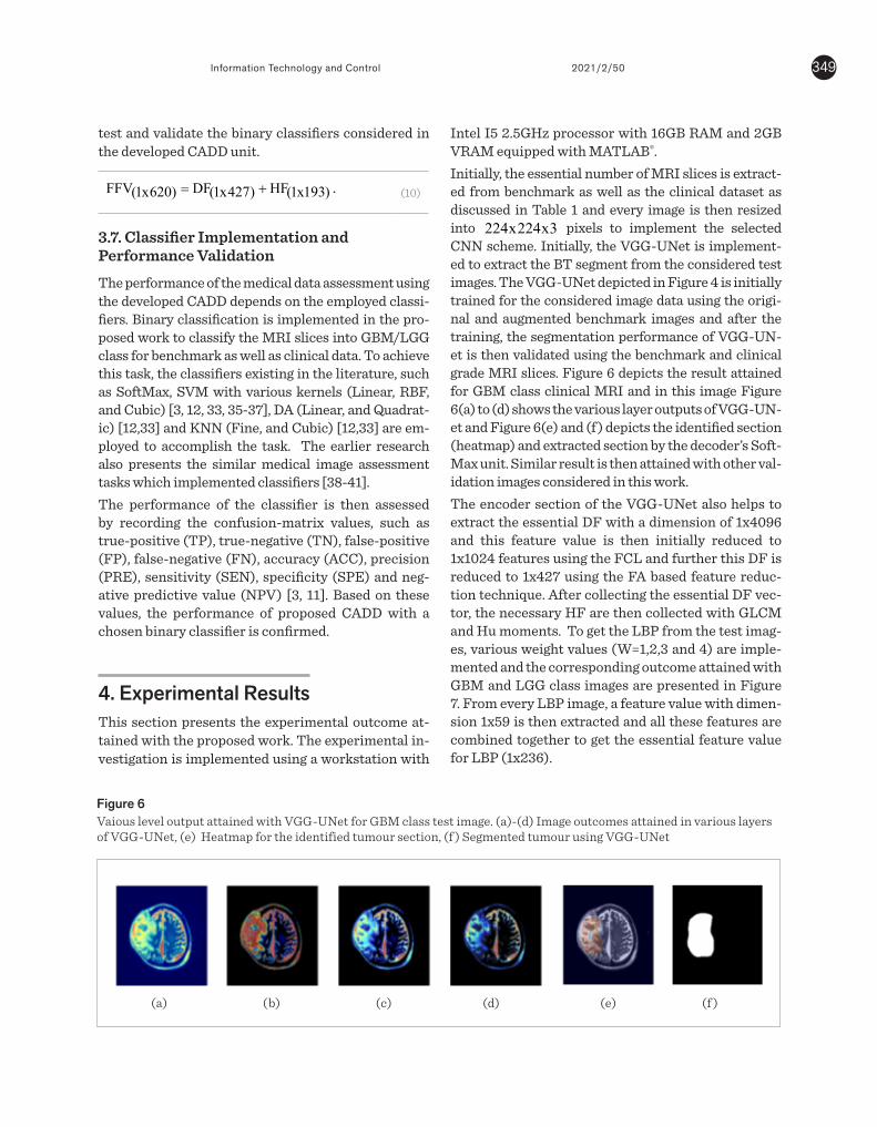
349Information Technology and Control 2021/2/50
test and validate the binary classifiers considered in the developed CADD unit.
discussed in [33].
The FA feature selection is implemented as follows;
Let us consider there exist feature vectors GBMFV and; let this vector is with a value of { }N1,0LGGFV,GBMFV ∈ . The FA then performs a feature wise assessment and computes the Hamming-Distance (HD) as in Equation (7):.
∑=
−=N
1aLGGaFVGBMaFV)LGGFV,GBMFV( HD , (7)
where N=1024 in DF and N=268 in HF
The difference in values between features is expressed as in Equation (8);
1iff ( , ) ( ).
N
GBM LGG GBMa LGGaa
D FV FV FV FV=
= −∑ (8)
The fitness function then assigned as in Equation (9):
max
1
( , )GBM LGGN
GBMa LGGaa
Fitnessvalue HD FV FV
FV FV=
= =
−∑
(9)
The )LGGFV,GBMFV( maxHD is then evaluated to decide the features and if 0)LGGFV,GBMFV( maxHD ≈ , then the particular feature is discarded and if max ( , ) 0,GBM LGGHD FV FV ≠ then the corresponding feature is selected and a new feature vector is formed. The proposed procedure is graphically presented in Figure 5 and the FA with optimally assigned parameters will help to identify the new feature vector.
Figure 5
Firefly algorithm based dominant feature selection
In this work, the FA with Brownian-Distribution is considered and other essential parameters are assigned as follows; number of fireflies=30, search dimension = total features, iterations=2500 and
other FA parameter information can be accessed from [34].
The FA based feature selection helped to get DF vector with a dimension of 1x427 and HF with a dimension of 1x193. These features are serially combined to get a new fused-feature-vector (FFV) depicted in Equation (10). This FFV is then considered to train, test and validate the binary classifiers considered in the developed CADD unit.
)193x1(HF)427x1(DF)620x1(FFV += . (10)
3.7 Classifier Implementation and Performance Validation
The performance of the medical data assessment using the developed CADD depends on the employed classifiers. Binary classification is implemented in the proposed work to classify the MRI slices into GBM/LGG class for benchmark as well as clinical data. To achieve this task, the classifiers existing in the literature, such as SoftMax, SVM with various kernels (Linear, RBF, and Cubic) [3, 12, 33, 35-37], DA (Linear, and Quadratic) [12,33] and KNN (Fine, and Cubic) [12,33] are employed to accomplish the task. The earlier research also presents the similar medical image assessment tasks which implemented classifiers [38-41].
The performance of the classifier is then assessed by recording the confusion-matrix values, such as true-positive (TP), true-negative (TN), false-positive (FP), false-negative (FN), accuracy (ACC), precision (PRE), sensitivity (SEN), specificity (SPE) and negative predictive value (NPV) [3, 11]. Based on these values, the performance of proposed CADD with a chosen binary classifier is confirmed.
4. Experimental Results This section presents the experimental outcome attained with the proposed work. The experimental investigation is implemented using a workstation with Intel I5 2.5GHz processor with 16GB RAM and 2GB VRAM equipped with MATLAB®.
Initially, the essential number of MRI slices is extracted from benchmark as well as the clinical dataset as discussed in Table 1 and every image is then resized into 3x224x224 pixels to implement the selected CNN
FA with optimally assigned
initial parameters
GBM
features
)FV,FV( HD LGGGBMmax
LGG
features
Selected feature
(10)
3.7. Classifier Implementation and Performance Validation
The performance of the medical data assessment using the developed CADD depends on the employed classi-fiers. Binary classification is implemented in the pro-posed work to classify the MRI slices into GBM/LGG class for benchmark as well as clinical data. To achieve this task, the classifiers existing in the literature, such as SoftMax, SVM with various kernels (Linear, RBF, and Cubic) [3, 12, 33, 35-37], DA (Linear, and Quadrat-ic) [12,33] and KNN (Fine, and Cubic) [12,33] are em-ployed to accomplish the task. The earlier research also presents the similar medical image assessment tasks which implemented classifiers [38-41].The performance of the classifier is then assessed by recording the confusion-matrix values, such as true-positive (TP), true-negative (TN), false-positive (FP), false-negative (FN), accuracy (ACC), precision (PRE), sensitivity (SEN), specificity (SPE) and neg-ative predictive value (NPV) [3, 11]. Based on these values, the performance of proposed CADD with a chosen binary classifier is confirmed.
4. Experimental ResultsThis section presents the experimental outcome at-tained with the proposed work. The experimental in-vestigation is implemented using a workstation with
Intel I5 2.5GHz processor with 16GB RAM and 2GB VRAM equipped with MATLAB®.Initially, the essential number of MRI slices is extract-ed from benchmark as well as the clinical dataset as discussed in Table 1 and every image is then resized into 3x224x224 pixels to implement the selected CNN scheme. Initially, the VGG-UNet is implement-ed to extract the BT segment from the considered test images. The VGG-UNet depicted in Figure 4 is initially trained for the considered image data using the origi-nal and augmented benchmark images and after the training, the segmentation performance of VGG-UN-et is then validated using the benchmark and clinical grade MRI slices. Figure 6 depicts the result attained for GBM class clinical MRI and in this image Figure 6(a) to (d) shows the various layer outputs of VGG-UN-et and Figure 6(e) and (f ) depicts the identified section (heatmap) and extracted section by the decoder’s Soft-Max unit. Similar result is then attained with other val-idation images considered in this work. The encoder section of the VGG-UNet also helps to extract the essential DF with a dimension of 1x4096 and this feature value is then initially reduced to 1x1024 features using the FCL and further this DF is reduced to 1x427 using the FA based feature reduc-tion technique. After collecting the essential DF vec-tor, the necessary HF are then collected with GLCM and Hu moments. To get the LBP from the test imag-es, various weight values (W=1,2,3 and 4) are imple-mented and the corresponding outcome attained with GBM and LGG class images are presented in Figure 7. From every LBP image, a feature value with dimen-sion 1x59 is then extracted and all these features are combined together to get the essential feature value for LBP (1x236).
scheme. Initially, the VGG-UNet is implemented to extract the BT segment from the considered test images. The VGG-UNet depicted in Figure 4 is initially trained for the considered image data using the original and augmented benchmark images and after the training, the segmentation performance of VGG-UNet is then validated using the benchmark and clinical grade MRI slices. Figure 6 depicts the result attained for GBM class clinical MRI and in this image Figure 6(a) to (d) shows the various layer outputs of VGG-UNet and Figure 6(e) and (f) depicts the identified section (heatmap) and extracted section by the decoder’s SoftMax unit. Similar result is then attained with other validation images considered in this work.
Figure 6
Vaious level output attained with VGG-UNet for GBM class test image. (a)-(d) Image outcomes attained in various layers of VGG-UNet, (e) Heatmap for the identified tumour section, (f) Segmented tumour using VGG-UNet
The encoder section of the VGG-UNet also helps to extract the essential DF with a dimension of 1x4096 and this feature value is then initially reduced to 1x1024 features using the FCL and further this DF is reduced to 1x427 using the FA based feature reduction technique. After collecting the essential DF vector, the necessary HF are then collected with GLCM and Hu moments. To get the LBP from the test images, various weight values (W=1,2,3 and 4) are implemented and the corresponding outcome attained with GBM and LGG class images are presented in Figure 7. From every LBP image, a feature value with dimension 1x59 is then extracted and all these features are combined together to get the essential feature value for LBP (1x236).
Figure 7
LBP treated brain MRI slices with chosen weights
Finally, the DF+HCF is implemented and the FFV is then considered to authenticate the classifiers and based on the attained confusion-matrix
parameters, the eminence of the proposed CADD is confirmed. During this classification task, a 10-fold cross validation is employed and the best result which is attained during the 10 trial is adopted as the best result by the considered classifier.
5. Discussion This section presents the merit of the proposed scheme on the considered image database. The performance of CADD is separately validated on the considered image datasets, initially CADD’s performance is tested using the TCIA database and the attained result is presented in Table 2 for DF alone and DF+HF.
The result presented in Table 2 depicts the results achieved with the binary classifier and the presented result confirms that the SVM classifier outperforms other classifier units, such as SoftMax, DA and KNN considered in this study. Figure 8 presents the Glyph-plot to demonstrate the classifier performance with DF along and DF+HF and from this figure, it can be noted that, the overall performance offered by the SVM-RBF in the case of DF (Figure 8(a)) and the performance by SVM-Cubic is better for DF+HF. This outcome confirms that, the classification accuracy of the CADD is improved due to the DF+HF compared to the classification accuracy by DF alone.
Table 2
The disease detection performance of CADD with TCIA database
Features Classifier TP FN TN FP ACC PRE SEN SPE NPV
DF
SoftMax 219 21 223 17 92.08 92.80 91.25 92.92 91.39
SVM-Linear 217 23 216 24 90.21 90.04 90.42 90.00 90.38
SVM-RBF 226 14 222 18 93.33 92.62 94.17 92.50 94.07
SVM-Cubic 221 19 225 15 92.92 93.64 92.08 93.75 92.21
DA-Linear 218 22 221 19 91.46 91.98 90.83 92.08 90.95
DA-Quadratic 220 20 218 22 91.25 90.91 91.67 90.83 91.60
KNN-Fine 224 16 222 18 92.92 92.56 93.33 92.50 93.28
KNN-Cubic 217 23 219 21 90.83 91.18 90.42 91.25 90.50
DF+
HF
SoftMax 230 10 227 13 95.21 94.65 95.83 94.58 95.78
SVM-Linear 228 12 223 17 93.96 93.06 95.00 92.92 94.89
SVM-RBF 225 15 231 9 95.00 96.15 93.75 96.25 93.90
SVM-Cubic 230 10 231 9 96.04 96.23 95.83 96.25 95.85
DA-Linear 231 9 223 17 94.58 93.15 96.25 92.92 96.12
DA-Quadratic 224 16 230 10 94.58 95.73 93.33 95.83 93.50
KNN-Fine 233 7 226 14 95.63 94.33 97.08 94.17 97.00
KNN-Cubic 228 12 229 11 95.21 95.40 95.00 95.42 95.02
Figure 8
Glyph-plot generated using the classifier
(a) (b) (c) (d) (e) (f )
Figure 6Vaious level output attained with VGG-UNet for GBM class test image. (a)-(d) Image outcomes attained in various layers of VGG-UNet, (e) Heatmap for the identified tumour section, (f ) Segmented tumour using VGG-UNet

Information Technology and Control 2021/2/50350
Figure 7 LBP treated brain MRI slices with chosen weights
Finally, the DF+HCF is implemented and the FFV is then considered to authenticate the classifiers and based on the attained confusion-matrix parameters, the eminence of the proposed CADD is confirmed. During this classification task, a 10-fold cross valida-tion is employed and the best result which is attained during the 10 trial is adopted as the best result by the considered classifier.
5. DiscussionThis section presents the merit of the proposed scheme on the considered image database. The per-formance of CADD is separately validated on the considered image datasets, initially CADD’s perfor-mance is tested using the TCIA database and the at-tained result is presented in Table 2 for DF alone and DF+HF. The result presented in Table 2 depicts the results achieved with the binary classifier and the presented result confirms that the SVM classifier outperforms other classifier units, such as SoftMax, DA and KNN considered in this study. Figure 8 presents the Glyph-plot to demonstrate the classifier performance with DF along and DF+HF and from this figure, it can be
scheme. Initially, the VGG-UNet is implemented to extract the BT segment from the considered test images. The VGG-UNet depicted in Figure 4 is initially trained for the considered image data using the original and augmented benchmark images and after the training, the segmentation performance of VGG-UNet is then validated using the benchmark and clinical grade MRI slices. Figure 6 depicts the result attained for GBM class clinical MRI and in this image Figure 6(a) to (d) shows the various layer outputs of VGG-UNet and Figure 6(e) and (f) depicts the identified section (heatmap) and extracted section by the decoder’s SoftMax unit. Similar result is then attained with other validation images considered in this work.
Figure 6
Vaious level output attained with VGG-UNet for GBM class test image. (a)-(d) Image outcomes attained in various layers of VGG-UNet, (e) Heatmap for the identified tumour section, (f) Segmented tumour using VGG-UNet
The encoder section of the VGG-UNet also helps to extract the essential DF with a dimension of 1x4096 and this feature value is then initially reduced to 1x1024 features using the FCL and further this DF is reduced to 1x427 using the FA based feature reduction technique. After collecting the essential DF vector, the necessary HF are then collected with GLCM and Hu moments. To get the LBP from the test images, various weight values (W=1,2,3 and 4) are implemented and the corresponding outcome attained with GBM and LGG class images are presented in Figure 7. From every LBP image, a feature value with dimension 1x59 is then extracted and all these features are combined together to get the essential feature value for LBP (1x236).
Figure 7
LBP treated brain MRI slices with chosen weights
Finally, the DF+HCF is implemented and the FFV is then considered to authenticate the classifiers and based on the attained confusion-matrix
parameters, the eminence of the proposed CADD is confirmed. During this classification task, a 10-fold cross validation is employed and the best result which is attained during the 10 trial is adopted as the best result by the considered classifier.
5. Discussion This section presents the merit of the proposed scheme on the considered image database. The performance of CADD is separately validated on the considered image datasets, initially CADD’s performance is tested using the TCIA database and the attained result is presented in Table 2 for DF alone and DF+HF.
The result presented in Table 2 depicts the results achieved with the binary classifier and the presented result confirms that the SVM classifier outperforms other classifier units, such as SoftMax, DA and KNN considered in this study. Figure 8 presents the Glyph-plot to demonstrate the classifier performance with DF along and DF+HF and from this figure, it can be noted that, the overall performance offered by the SVM-RBF in the case of DF (Figure 8(a)) and the performance by SVM-Cubic is better for DF+HF. This outcome confirms that, the classification accuracy of the CADD is improved due to the DF+HF compared to the classification accuracy by DF alone.
Table 2
The disease detection performance of CADD with TCIA database
Features Classifier TP FN TN FP ACC PRE SEN SPE NPV
DF
SoftMax 219 21 223 17 92.08 92.80 91.25 92.92 91.39
SVM-Linear 217 23 216 24 90.21 90.04 90.42 90.00 90.38
SVM-RBF 226 14 222 18 93.33 92.62 94.17 92.50 94.07
SVM-Cubic 221 19 225 15 92.92 93.64 92.08 93.75 92.21
DA-Linear 218 22 221 19 91.46 91.98 90.83 92.08 90.95
DA-Quadratic 220 20 218 22 91.25 90.91 91.67 90.83 91.60
KNN-Fine 224 16 222 18 92.92 92.56 93.33 92.50 93.28
KNN-Cubic 217 23 219 21 90.83 91.18 90.42 91.25 90.50
DF+
HF
SoftMax 230 10 227 13 95.21 94.65 95.83 94.58 95.78
SVM-Linear 228 12 223 17 93.96 93.06 95.00 92.92 94.89
SVM-RBF 225 15 231 9 95.00 96.15 93.75 96.25 93.90
SVM-Cubic 230 10 231 9 96.04 96.23 95.83 96.25 95.85
DA-Linear 231 9 223 17 94.58 93.15 96.25 92.92 96.12
DA-Quadratic 224 16 230 10 94.58 95.73 93.33 95.83 93.50
KNN-Fine 233 7 226 14 95.63 94.33 97.08 94.17 97.00
KNN-Cubic 228 12 229 11 95.21 95.40 95.00 95.42 95.02
Figure 8
Glyph-plot generated using the classifier
W= 1
LGG
GBM
W= 2 W= 3 W= 4
noted that, the overall performance offered by the SVM-RBF in the case of DF (Figure 8(a)) and the per-formance by SVM-Cubic is better for DF+HF. This outcome confirms that, the classification accuracy of the CADD is improved due to the DF+HF compared to the classification accuracy by DF alone. Related practice is then repeated with the clinical MRI dataset and the attained results are present-ed in Table 3. From Table 3, it can be noted that the SVM-Cubic classifier helped to achieve better clas-sification accuracy with DF and DF+HF feature vec-tors. The confusion matrix presented in Figure 9 (a) and (b) also confirms the eminence of the SVM-Cu-bic classifier compared to other methods. Further, the Receiver Operating Characteristic (ROC) curve pre-sented in Figure 9(c) confirms that the SVM-Cubic offers better result with DF+HF compared to other SVM, DA, KNN and SoftMax classifiers considered in this work.The overall performance of the CADD is then present-ed in Figure 10 using the Glyph-plot and this figure also confirms that the performance of the SSM-Cubic is better with the clinical images for DF and DF+HF. These results confirm that, proposed CNN based seg-mentation and SVM classification is clinically note-worthy and the developed CADD can be considered to

351Information Technology and Control 2021/2/50
Table 2The disease detection performance of CADD with TCIA database
Features Classifier TP FN TN FP ACC PRE SEN SPE NPV
DF
SoftMax 219 21 223 17 92.08 92.80 91.25 92.92 91.39
SVM-Linear 217 23 216 24 90.21 90.04 90.42 90.00 90.38
SVM-RBF 226 14 222 18 93.33 92.62 94.17 92.50 94.07
SVM-Cubic 221 19 225 15 92.92 93.64 92.08 93.75 92.21
DA-Linear 218 22 221 19 91.46 91.98 90.83 92.08 90.95
DA-Quadratic 220 20 218 22 91.25 90.91 91.67 90.83 91.60
KNN-Fine 224 16 222 18 92.92 92.56 93.33 92.50 93.28
KNN-Cubic 217 23 219 21 90.83 91.18 90.42 91.25 90.50
DF+
HF
SoftMax 230 10 227 13 95.21 94.65 95.83 94.58 95.78
SVM-Linear 228 12 223 17 93.96 93.06 95.00 92.92 94.89
SVM-RBF 225 15 231 9 95.00 96.15 93.75 96.25 93.90
SVM-Cubic 230 10 231 9 96.04 96.23 95.83 96.25 95.85
DA-Linear 231 9 223 17 94.58 93.15 96.25 92.92 96.12
DA-Quadratic 224 16 230 10 94.58 95.73 93.33 95.83 93.50
KNN-Fine 233 7 226 14 95.63 94.33 97.08 94.17 97.00
KNN-Cubic 228 12 229 11 95.21 95.40 95.00 95.42 95.02
Figure 8Glyph-plot generated using the classifier performance for TCIA image database
performance for TCIA image database
SoftMax SVM-Linear SVM-RBF SVM-Cubic
DA-Linear DA-Quadratic KNN-Fine KNN-Cubic
(a) DF
SoftMax SVM-Linear SVM-RBF SVM-Cubic
DA-Linear DA-Quadratic KNN-Fine KNN-Cubic
(b) DF+HF
Table 3
Brain tumour detection performance of CADD with clinical images Features Classifier TP FN TN FP ACC PRE SEN SPE NPV
DF
SoftMax 82 8 84 6 92.22 93.18 91.11 93.33 91.30
SVM-Linear 85 5 81 9 92.22 90.43 94.44 90.00 94.19
SVM-RBF 83 7 80 10 90.56 89.25 92.22 88.89 91.95
SVM-Cubic 85 5 83 7 93.33 92.39 94.44 92.22 94.32
DA-Linear 81 9 86 4 92.78 95.29 90.00 95.56 90.53
DA-Quadratic 83 7 85 5 93.33 94.32 92.22 94.44 92.39
KNN-Fine 84 6 82 8 92.22 91.30 93.33 91.11 93.18
KNN-Cubic 86 4 81 9 92.78 90.53 95.56 90.00 95.29
DF+
HF
SoftMax 85 5 85 5 94.44 94.44 94.44 94.44 94.44
SVM-Linear 86 4 88 2 96.67 97.73 95.56 97.78 95.65
SVM-RBF 88 2 87 3 97.22 96.70 97.78 96.67 97.75
SVM-Cubic 89 1 89 1 98.89 98.88 98.88 98.88 98.88
DA-Linear 86 4 85 5 95.00 94.51 95.56 94.44 95.51
DA-Quadratic 89 1 88 2 98.33 97.80 98.89 97.78 98.88
KNN-Fine 88 2 89 1 98.33 98.88 97.78 98.89 97.80
KNN-Cubic 88 2 88 2 97.78 97.78 97.78 97.78 97.78
Figure 9
SVM-Cubic performance for clinical MRI database
GBMLG
G
Target Class
GBM
LGG
Out
put C
lass
Confusion Matrix
85
47.2%
5
2.8%
94.4%
5.6%
7
3.9%
83
46.1%
92,2%
7.8%
92.4%
7.6%
94.3%
5.7%
93.3%
6.7%
(a) DF and SVM-
Cubic
GBMLG
G
Target Class
GBM
LGG
Out
put C
lass
Confusion Matrix
89
49.1%
1
0.9%
98.9%
1.1%
1
0.9%
89
49.1%
98.9%
1.1%
98.9%
1.1%
98.9%
1.1%
98.9%
1.1%
(b) DF+HF with SVM-
Cubic
0 20 40 60 80 100
100-Specificity
0
20
40
60
80
100
Sens
itivi
ty
SoftMax
SVM-Linear
SVM-RBF
SVM-Cubic
DA-Linear
DA-Quadratic
KNN-Fine
KNN-Cubic
(c) ROC curve for DF+HF
Related practice is then repeated with the clinical MRI dataset and the attained results are presented in Table 3. From Table 3, it can be noted that the SVM-Cubic classifier helped to achieve better classification accuracy with DF and DF+HF feature vectors. The confusion matrix presented in Figure 9 (a) and (b) also confirms the eminence of the SVM-Cubic classifier compared to other methods. Further, the Receiver Operating Characteristic (ROC) curve presented in Figure 9(c) confirms that the SVM-Cubic offers better result with DF+HF compared to other SVM, DA, KNN and SoftMax classifiers considered in this work.
Figure 10
Glyph-plot generated using the classifier performance for clinical MRI database
SoftMax SVM-Linear SVM-RBF SVM-Cubic
DA-Linear DA-Quadratic KNN-Fine KNN-Cubic
(a) DF
SoftMax SVM-Linear SVM-RBF SVM-Cubic
DA-Linear DA-Quadratic KNN-Fine KNN-Cubic
(b) DF+HF
The overall performance of the CADD is then presented in Figure 10 using the Glyph-plot and this figure also confirms that the
(a) DF (b) DF+HF
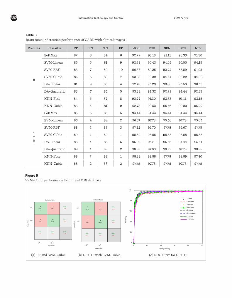
Information Technology and Control 2021/2/50352
Figure 9SVM-Cubic performance for clinical MRI database
Table 3Brain tumour detection performance of CADD with clinical images
Features Classifier TP FN TN FP ACC PRE SEN SPE NPV
DF
SoftMax 82 8 84 6 92.22 93.18 91.11 93.33 91.30
SVM-Linear 85 5 81 9 92.22 90.43 94.44 90.00 94.19
SVM-RBF 83 7 80 10 90.56 89.25 92.22 88.89 91.95
SVM-Cubic 85 5 83 7 93.33 92.39 94.44 92.22 94.32
DA-Linear 81 9 86 4 92.78 95.29 90.00 95.56 90.53
DA-Quadratic 83 7 85 5 93.33 94.32 92.22 94.44 92.39
KNN-Fine 84 6 82 8 92.22 91.30 93.33 91.11 93.18
KNN-Cubic 86 4 81 9 92.78 90.53 95.56 90.00 95.29
DF+
HF
SoftMax 85 5 85 5 94.44 94.44 94.44 94.44 94.44
SVM-Linear 86 4 88 2 96.67 97.73 95.56 97.78 95.65
SVM-RBF 88 2 87 3 97.22 96.70 97.78 96.67 97.75
SVM-Cubic 89 1 89 1 98.89 98.88 98.88 98.88 98.88
DA-Linear 86 4 85 5 95.00 94.51 95.56 94.44 95.51
DA-Quadratic 89 1 88 2 98.33 97.80 98.89 97.78 98.88
KNN-Fine 88 2 89 1 98.33 98.88 97.78 98.89 97.80
KNN-Cubic 88 2 88 2 97.78 97.78 97.78 97.78 97.78
performance for TCIA image database
SoftMax SVM-Linear SVM-RBF SVM-Cubic
DA-Linear DA-Quadratic KNN-Fine KNN-Cubic
(a) DF
SoftMax SVM-Linear SVM-RBF SVM-Cubic
DA-Linear DA-Quadratic KNN-Fine KNN-Cubic
(b) DF+HF
Table 3
Brain tumour detection performance of CADD with clinical images Features Classifier TP FN TN FP ACC PRE SEN SPE NPV
DF
SoftMax 82 8 84 6 92.22 93.18 91.11 93.33 91.30
SVM-Linear 85 5 81 9 92.22 90.43 94.44 90.00 94.19
SVM-RBF 83 7 80 10 90.56 89.25 92.22 88.89 91.95
SVM-Cubic 85 5 83 7 93.33 92.39 94.44 92.22 94.32
DA-Linear 81 9 86 4 92.78 95.29 90.00 95.56 90.53
DA-Quadratic 83 7 85 5 93.33 94.32 92.22 94.44 92.39
KNN-Fine 84 6 82 8 92.22 91.30 93.33 91.11 93.18
KNN-Cubic 86 4 81 9 92.78 90.53 95.56 90.00 95.29
DF+
HF
SoftMax 85 5 85 5 94.44 94.44 94.44 94.44 94.44
SVM-Linear 86 4 88 2 96.67 97.73 95.56 97.78 95.65
SVM-RBF 88 2 87 3 97.22 96.70 97.78 96.67 97.75
SVM-Cubic 89 1 89 1 98.89 98.88 98.88 98.88 98.88
DA-Linear 86 4 85 5 95.00 94.51 95.56 94.44 95.51
DA-Quadratic 89 1 88 2 98.33 97.80 98.89 97.78 98.88
KNN-Fine 88 2 89 1 98.33 98.88 97.78 98.89 97.80
KNN-Cubic 88 2 88 2 97.78 97.78 97.78 97.78 97.78
Figure 9
SVM-Cubic performance for clinical MRI database
GBMLG
G
Target Class
GBM
LGG
Out
put C
lass
Confusion Matrix
85
47.2%
5
2.8%
94.4%
5.6%
7
3.9%
83
46.1%
92,2%
7.8%
92.4%
7.6%
94.3%
5.7%
93.3%
6.7%
(a) DF and SVM-
Cubic
GBMLG
G
Target Class
GBM
LGG
Out
put C
lass
Confusion Matrix
89
49.1%
1
0.9%
98.9%
1.1%
1
0.9%
89
49.1%
98.9%
1.1%
98.9%
1.1%
98.9%
1.1%
98.9%
1.1%
(b) DF+HF with SVM-
Cubic
0 20 40 60 80 100
100-Specificity
0
20
40
60
80
100
Sens
itivi
ty
SoftMax
SVM-Linear
SVM-RBF
SVM-Cubic
DA-Linear
DA-Quadratic
KNN-Fine
KNN-Cubic
(c) ROC curve for DF+HF
Related practice is then repeated with the clinical MRI dataset and the attained results are presented in Table 3. From Table 3, it can be noted that the SVM-Cubic classifier helped to achieve better classification accuracy with DF and DF+HF feature vectors. The confusion matrix presented in Figure 9 (a) and (b) also confirms the eminence of the SVM-Cubic classifier compared to other methods. Further, the Receiver Operating Characteristic (ROC) curve presented in Figure 9(c) confirms that the SVM-Cubic offers better result with DF+HF compared to other SVM, DA, KNN and SoftMax classifiers considered in this work.
Figure 10
Glyph-plot generated using the classifier performance for clinical MRI database
SoftMax SVM-Linear SVM-RBF SVM-Cubic
DA-Linear DA-Quadratic KNN-Fine KNN-Cubic
(a) DF
SoftMax SVM-Linear SVM-RBF SVM-Cubic
DA-Linear DA-Quadratic KNN-Fine KNN-Cubic
(b) DF+HF
The overall performance of the CADD is then presented in Figure 10 using the Glyph-plot and this figure also confirms that the
(a) DF and SVM-Cubic (b) DF+HF with SVM-Cubic (c) ROC curve for DF+HF
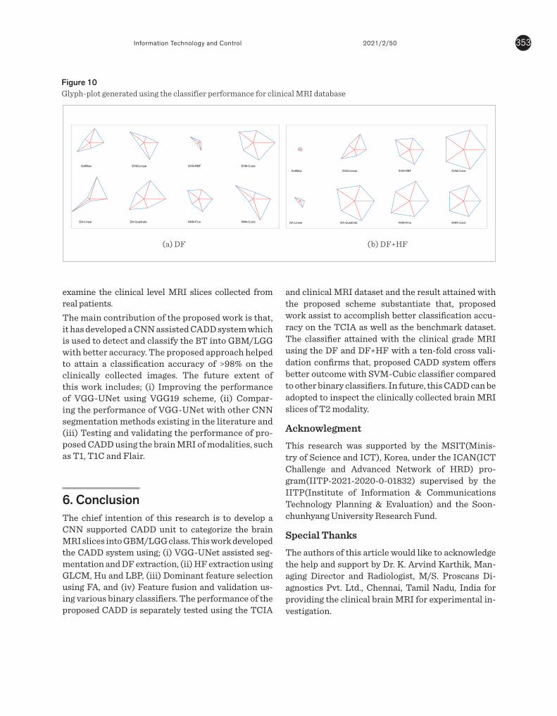
353Information Technology and Control 2021/2/50
Figure 10Glyph-plot generated using the classifier performance for clinical MRI database
examine the clinical level MRI slices collected from real patients.The main contribution of the proposed work is that, it has developed a CNN assisted CADD system which is used to detect and classify the BT into GBM/LGG with better accuracy. The proposed approach helped to attain a classification accuracy of >98% on the clinically collected images. The future extent of this work includes; (i) Improving the performance of VGG-UNet using VGG19 scheme, (ii) Compar-ing the performance of VGG-UNet with other CNN segmentation methods existing in the literature and (iii) Testing and validating the performance of pro-posed CADD using the brain MRI of modalities, such as T1, T1C and Flair.
6. ConclusionThe chief intention of this research is to develop a CNN supported CADD unit to categorize the brain MRI slices into GBM/LGG class. This work developed the CADD system using; (i) VGG-UNet assisted seg-mentation and DF extraction, (ii) HF extraction using GLCM, Hu and LBP, (iii) Dominant feature selection using FA, and (iv) Feature fusion and validation us-ing various binary classifiers. The performance of the proposed CADD is separately tested using the TCIA
performance for TCIA image database
SoftMax SVM-Linear SVM-RBF SVM-Cubic
DA-Linear DA-Quadratic KNN-Fine KNN-Cubic
(a) DF
SoftMax SVM-Linear SVM-RBF SVM-Cubic
DA-Linear DA-Quadratic KNN-Fine KNN-Cubic
(b) DF+HF
Table 3
Brain tumour detection performance of CADD with clinical images Features Classifier TP FN TN FP ACC PRE SEN SPE NPV
DF
SoftMax 82 8 84 6 92.22 93.18 91.11 93.33 91.30
SVM-Linear 85 5 81 9 92.22 90.43 94.44 90.00 94.19
SVM-RBF 83 7 80 10 90.56 89.25 92.22 88.89 91.95
SVM-Cubic 85 5 83 7 93.33 92.39 94.44 92.22 94.32
DA-Linear 81 9 86 4 92.78 95.29 90.00 95.56 90.53
DA-Quadratic 83 7 85 5 93.33 94.32 92.22 94.44 92.39
KNN-Fine 84 6 82 8 92.22 91.30 93.33 91.11 93.18
KNN-Cubic 86 4 81 9 92.78 90.53 95.56 90.00 95.29
DF+
HF
SoftMax 85 5 85 5 94.44 94.44 94.44 94.44 94.44
SVM-Linear 86 4 88 2 96.67 97.73 95.56 97.78 95.65
SVM-RBF 88 2 87 3 97.22 96.70 97.78 96.67 97.75
SVM-Cubic 89 1 89 1 98.89 98.88 98.88 98.88 98.88
DA-Linear 86 4 85 5 95.00 94.51 95.56 94.44 95.51
DA-Quadratic 89 1 88 2 98.33 97.80 98.89 97.78 98.88
KNN-Fine 88 2 89 1 98.33 98.88 97.78 98.89 97.80
KNN-Cubic 88 2 88 2 97.78 97.78 97.78 97.78 97.78
Figure 9
SVM-Cubic performance for clinical MRI database
GBMLG
G
Target Class
GBM
LGG
Out
put C
lass
Confusion Matrix
85
47.2%
5
2.8%
94.4%
5.6%
7
3.9%
83
46.1%
92,2%
7.8%
92.4%
7.6%
94.3%
5.7%
93.3%
6.7%
(a) DF and SVM-
Cubic
GBMLG
G
Target Class
GBM
LGG
Out
put C
lass
Confusion Matrix
89
49.1%
1
0.9%
98.9%
1.1%
1
0.9%
89
49.1%
98.9%
1.1%
98.9%
1.1%
98.9%
1.1%
98.9%
1.1%
(b) DF+HF with SVM-
Cubic
0 20 40 60 80 100
100-Specificity
0
20
40
60
80
100
Sens
itivi
ty
SoftMax
SVM-Linear
SVM-RBF
SVM-Cubic
DA-Linear
DA-Quadratic
KNN-Fine
KNN-Cubic
(c) ROC curve for DF+HF
Related practice is then repeated with the clinical MRI dataset and the attained results are presented in Table 3. From Table 3, it can be noted that the SVM-Cubic classifier helped to achieve better classification accuracy with DF and DF+HF feature vectors. The confusion matrix presented in Figure 9 (a) and (b) also confirms the eminence of the SVM-Cubic classifier compared to other methods. Further, the Receiver Operating Characteristic (ROC) curve presented in Figure 9(c) confirms that the SVM-Cubic offers better result with DF+HF compared to other SVM, DA, KNN and SoftMax classifiers considered in this work.
Figure 10
Glyph-plot generated using the classifier performance for clinical MRI database
SoftMax SVM-Linear SVM-RBF SVM-Cubic
DA-Linear DA-Quadratic KNN-Fine KNN-Cubic
(a) DF
SoftMax SVM-Linear SVM-RBF SVM-Cubic
DA-Linear DA-Quadratic KNN-Fine KNN-Cubic
(b) DF+HF
The overall performance of the CADD is then presented in Figure 10 using the Glyph-plot and this figure also confirms that the
(a) DF (b) DF+HF
and clinical MRI dataset and the result attained with the proposed scheme substantiate that, proposed work assist to accomplish better classification accu-racy on the TCIA as well as the benchmark dataset. The classifier attained with the clinical grade MRI using the DF and DF+HF with a ten-fold cross vali-dation confirms that, proposed CADD system offers better outcome with SVM-Cubic classifier compared to other binary classifiers. In future, this CADD can be adopted to inspect the clinically collected brain MRI slices of T2 modality.
Acknowlegment
This research was supported by the MSIT(Minis-try of Science and ICT), Korea, under the ICAN(ICT Challenge and Advanced Network of HRD) pro-gram(IITP-2021-2020-0-01832) supervised by the IITP(Institute of Information & Communications Technology Planning & Evaluation) and the Soon-chunhyang University Research Fund.
Special Thanks
The authors of this article would like to acknowledge the help and support by Dr. K. Arvind Karthik, Man-aging Director and Radiologist, M/S. Proscans Di-agnostics Pvt. Ltd., Chennai, Tamil Nadu, India for providing the clinical brain MRI for experimental in-vestigation.
Information Technology and Control 2021/2/50354
References 1. Acharya, U. R., Fernandes, S. L., Weikoh, J. E., Ciaccio, E.
J., Fabell, M. K. M., Tanik, U. J., Rajinikanth, V., Yeong, C. H. Automated Detection of Alzheimer's Disease Using Brain MRI Images-A Study with Various Feature Ex-traction Techniques. Journal of Medical Systems, 2019, 43(9), 302. https://doi.org/10.1007/s10916-019-1428-9
2. Bakiya, A., Kamalanand, K., Rajinikanth, V., Nayak, R., Kadry, S. Deep Neural Network Assisted Diagnosis of Time-Frequency Transformed Electromyograms. Mul-timedia Tools and Applications, 2020, 79(15), 11051-67. https://doi.org/10.1007/s11042-018-6561-9
3. Balakrishna, C., Dadashzadeh, S., Soltaninejad, S. Au-tomatic Detection of Lumen and Media in the Ivus Im-ages Using U-net with Vgg16 Encoder. Arxiv Preprint Arxiv:1806.07554. 2018.
4. Bhandary, A., Prabhu, G., Rajinikanth, V., Thanaraj, K., Satapathy, S., Robbins, D. E., Shasky, C., Zhang, Y.-D., Ta-vares, J., M, R. S., Raja, N. S. M. Deep-Learning Frame-work to Detect Lung Abnormality-A Study With Chest X-ray and Lung CT Scan Images. Pattern Recognition Letters, 2020, 129, 271-8.https://doi.org/10.1016/j.pa-trec.2019.11.013
5. Clark, K., Vendt, B., Smith, K., Freymann, J., Kirby, J., Koppel, P., Moore, S., Phillips, S., Maffitt, D., Pringle, M., Tarbox, L., Prior, F. The Cancer Imaging Archive (TCIA): Maintaining and Operating a Public Informa-tion Repository. Journal of Digital Imaging, 2013, 26(6), 1045-57. https://doi.org/10.1007/s10278-013-9622-7
6. Dey, N., Rajinikanth, V., Shi, F., Tavares, J., Moraru, L., Karthik, K. A., Kamalanand, K., Emmanuel, C. So-cial-Group-Optimization Based Tumor Evaluation Tool for Clinical Brain MRI of Flair/Diffusion-Weighted Mo-dality. Biocybernetics and Biomedical Engineering, 2019, 39(3), 843-56. https://doi.org/10.1016/j.bbe.2019.07.005
7. Fernandes, S., Tanik, U., Rajinikanth, V., Karthik, K. A Reliable Framework for Accurate Brain Image Ex-amination and Treatment Planning Based on Early Diagnosis Support for Clinicians. Neural Computing and Applications, 2020, 32(20), 15897-908. https://doi.org/10.1007/s00521-019-04369-5
8. Godse, R., Bhat, S. Combined Morphology and SVM-Based Fault Feature Extraction Technique for Detection and Classification of Transmission Line Faults. Turkish Journal of Electrical Engineering & Computer Sciences, 2020, 28(5), 2768-88. https://doi.org/10.3906/elk-1912-7
9. Gudigar, A., Raghavendra, U., Devasia, T., Nayak, K., Dan-ish, S., Kamath, G., Samanth, J., Pai, U. M., Naya, V., Tan,
R. S., Ciaccio, E. J., Acharya, U. R. Global Weighted LBP Based Entropy Features for the Assessment of Pulmo-nary Hypertension. Pattern Recognition Letters, 2019, 125, 35-41. https://doi.org/10.1016/j.patrec.2019.03.027
10. Gülgün, O., Hamza, E. Classification Performance Com-parisons of Deep Learning Models in Pneumonia Diag-nosis Using Chest X-ray Images. Turkish Journal of En-gineering, 2020, 4(3), 129-141.https://doi.org/10.31127/tuje.652358
11. Hussain, U., Khan, M., Lali, I., Javed, K., Ashraf, I., Tariq, J., Ali, H., Din, A. A Unified Design of Aco and Skewness Based Brain Tumor Segmentation and Classification from MRI Scans. Journal of Control Engineering and Applied Informatics, 2020, 22(2), 43-55.
12. Jafarpour, S., Sedghi, Z., Amirani, M. A Robust Brain MRI Classification with GLCM Features. Internation-al Journal of Computer Applications, 2012, 37(12), 1-5. https://doi.org/10.5120/4735-6872.
13. Jiao, L., Huo, L., Hu, C., Tang, P. Refined Unet V2: End-to-End Patch-Wise Network for Noise-Free Cloud and Shadow Segmentation. Remote Sensing, 2020, 12(21), 3530. https://doi.org/10.3390/rs12213530
14. Kallenberg, K., Bock, H., Helms, G., Jung, K., Wrede, A., Buhk, J.-H., Giese, A., Frahm, J., Strik, H., Dechent, P., Knauth, M. Untreated Glioblastoma Multiforme: In-creased Myo-inositol and Glutamine Levels in the Con-tralateral Cerebral Hemisphere at Proton MRI Spec-troscopy. Radiology, 2009, 253(3), 805-812. https://doi.org/10.1148/radiol.2533071654
15. Karimi, D., Dou, H., Warfield, S. K., Gholipour, A. Deep Learning with Noisy Labels: Exploring Techniques and Remedies in Medical Image Analysis. Medical Image Analysis, 2020, 65, 101759. https://doi.org/10.1016/j.media.2020.101759
16. Ke, Q., Zhang, J., Wei, W., Damaševičius, R., Woźniak, M. Adaptive Independent Subspace Analysis of Brain Mag-netic Resonance Imaging Data. Ieee Access, 2019, 7, 12252-12261. https://doi.org/10.1109/ACCESS.2019.2893496
17. Khan, M., Ashraf, I., Alhaisoni, M., Damaševičius, R., Scherer, R. Et Al. Multimodal Brain Tumor Classifica-tion Using Deep Learning and Robust Feature Selec-tion: A Machine Learning Application for Radiologists. Diagnostics, 2020, 10(8), 565. https://doi.org/10.3390/diagnostics10080565
18. Khan, M., Kadry, S., Alhaisoni, M., Nam, Y., Zhang, Y., Rajinikanth, V., Sarfraz, M. S. Computer-Aided Gas-trointestinal Diseases Analysis from Wireless Capsule

355Information Technology and Control 2021/2/50
Endoscopy: A Framework of Best Features Selection. IEEE Access, 2020, 8, 132850-132859. https://doi.org/10.1109/ACCESS.2020.3010448
19. Khan, M., Rubab, S., Kashif, A., Sharif, M., Muhammad, N., Shah, J. H., Zhang, Y.-D., Satapathy, S. C. Lungs Can-cer Classification from CT Images: An Integrated De-sign of Contrast Based Classical Features Fusion and Selection. Pattern Recognition Letters, 2020, 129, 77-85. https://doi.org/10.1016/j.patrec.2019.11.014
20. Khan, M. A., Sarfraz, M. S., Alhaisoni, M., Albesher, A. A., Wang, S., Ashraf, I.. Stomachnet: Optimal Deep Learn-ing Features Fusion for Stomach Abnormalities Clas-sification. IEEE Access, 2020. https://doi.org/10.1109/ACCESS.2020.3034217
21. Khan, S., Nazir, M., Khan, M., Saba, T., Javed, K., Rehman, A., Akram, T., Awais, M. Lungs Nodule Detection Frame-work from Computed Tomography Images Using Sup-port Vector Machine. Microscopy Research and Tech-nique, 2019, 82(8), 1256-1266.https://doi.org/10.1002/jemt.23275
22. Louis, D., Perry, A., Reifenberger, G., Deimling, V., Figarel-la-Branger, D., Cavenee, W. K., Ohgaki, H., Wiestler, O. D., Kleihues, P., Ellison, D. W. The 2016 World Health Orga-nization Classification of Tumors of the Central Nervous System: A Summary. Acta Neuropathologica, 2016, 131(6), 803-820. https://doi.org/10.1007/s00401-016-1545-1
23. Nazar, U., Khan, M., Lali, I., Lin, H., Ali, H., Ashraf, I., T., J. Review of Automated Computerized Methods for Brain Tumor Segmentation and Classification. Current Medical Imaging, 2020, 16(7), 823-34. https://doi.org/10.2174/1573405615666191120110855
24. Öztürk, Ş. Stacked Auto-Encoder Based Tagging with Deep Features for Content-Based Medical Image Re-trieval. Expert Systems with Applications, 2020, 161, 113693. https://doi.org/10.1016/j.eswa.2020.113693
25. Pedano, N., Flanders, A., Scarpace, L., Mikkelsen, T., Es-chbacher, J. M., Hermes, B., Ostrom, Q. Radiology Data from the Cancer Genome Atlas Low Grade Glioma [tc-ga-lgg] Collection. The Cancer Imaging Archive, 2016. http://doi.org/10.7937/k9/tcia.2016.l4ltd3tk.
26. Połap, D. An Adaptive Genetic Algorithm as a Support-ing Mechanism for Microscopy Image Analysis in a Cascade of Convolution Neural Networks. Applied Soft Computing, 2020, 97, 106824. https://doi.org/10.1016/j.asoc.2020.106824
27. Połap, D. Analysis of Skin Marks Through the use of In-telligent Things. IEEE Access, 2019; 7, 149355-149363. https://doi.org/10.1109/ACCESS.2019.2947354
28. Pugalenthi, R., Rajakumar, M., Ramya, J., Rajinikanth, V. Evaluation and Classification of the Brain Tumor MRI Using Machine Learning Technique. Journal of Control Engineering and Applied Informatics, 2019, 21(4), 12-21.
29. Qureshi, S., Karilla, S., Vanichayobon, S. Gacnn Sleep-tunenet: A Genetic Algorithm Designing the Convo-lutional Neural Network Architecture for Optimal Classification of Sleep Stages from a Single EEG Channel. Turkish Journal of Electrical Engineering & Computer Sciences, 2019, 27(6), 4203-419. https://doi.org/10.3906/elk-1903-186
30. Raja, S., Rajinikanth, V., Latha, K. Otsu Based Optimal Multilevel Image Thresholding Using Firefly Algo-rithm. Modelling and Simulation in Engineering, 2014. https://doi.org/10.1155/2014/794574
31. Rajinikanth, V., Raj, J., Thanaraj, K., Naik, G. A Cus-tomized Vgg19 Network with Concatenation of Deep and Handcrafted Features for Brain Tumor Detec-tion. Applied Sciences, 2020, 10(10), 3429. https://doi.org/10.3390/app10103429
32. Rajinikanth, V., Satapathy, S. Segmentation of Ischemic Stroke Lesion in Brain MRI Based on Social Group Op-timization and Fuzzy-tsallis Entropy. Arabian Journal for Science and Engineering, 2018, 43(8), 4365-478. https://doi.org/10.1007/s13369-017-3053-6
33. Rehman, A., Khan, M., Saba, T., Mehmood, Z., Tariq, U., Ayesha, N. Microscopic Brain Tumor Detection and Classification Using 3D CNN and Feature Selection Ar-chitecture. Microscopy Research and Technique, 2020. https://doi.org/10.1002/jemt.23597
34. Ronneberger, O., Fischer, P., Brox, T. U-net: Convolu-tional Networks for Biomedical Image Segmentation. In: Navab, N., Hornegger, J., Wells, W., Frangi, A. (Eds.) Medical Image Computing and Computer-Assist-ed Intervention - Miccai 2015. Miccai 2015. Lecture Notes in Computer Science, 2015, 9351. https://doi.org/10.1007/978-3-319-24574-4_28
35. Saba, T., Mohamed, A., El-affendi, M., Amin, J., Sharif, M. Brain Tumor Detection Using Fusion of Hand Craft-ed and Deep Learning Features. Cognitive Systems Research, 2020, 59, 221-230. https://doi.org/10.1016/j.cogsys.2019.09.007
36. Sabhara, R., Lee, C., Lim, K. Comparative Study of Hu Moments and Zernike Moments in Object Recognition. SMARTCR, 2013, 3(3), 166-173. https://doi.org/10.6029/smartcr.2013.03.003
37. Scarpace, L., Mikkelsen, T., Cha, S., Rao, S., Tekchan-dani, S., et al. Radiology Data from the Cancer Genome

Information Technology and Control 2021/2/50356
Atlas Glioblastoma Multiforme [tcga-gbm] Collec-tion. The Cancer Imaging Archive, 2016. http://doi.org/10.7937/k9/tcia.2016.rnyfuye9
38. Sharif, M., L, J., Khan, M., Salee, M. Active Deep Neural Network Features Selection for Segmentation and Rec-ognition of Brain Tumors Using MRI Images. Pattern Recognition Letters, 2020, 129, 181-189. https://doi.org/10.1016/j.patrec.2019.11.019
39. Vlis, V., Hoeben, A., Beckervordersandforth, J., Acker-mans, L., Eekers, D., Wennekes, R. M. J., Schijns, O. E. M. G. Impact of the Revised Who Classification of Dif-
fuse Low-Grade Glioma on Clinical Decision Making: A Case Report. Surgical Neurology International, 2017, 8. https://doi.org/10.4103/sni.sni_166_17
40. Yasrab, R. ECRU: An Encoder-Decoder Based Convo-lution Neural Network (CNN) for Road-Scene Under-standing. Journal of Imaging, 2018, 10, 116. https://doi.org/10.3390/jimaging4100116
41. Yushkevich, P., Piven, J., Hazlett, H., Smith, R., Ho, S. User-Guided 3D Active Contour Segmentation of An-atomical Structures: Significantly Improved Efficien-cy and Reliability. Neuroimage, 2006, 31(3), 1116-128. https://doi.org/10.1016/j.neuroimage.2006.01.015
This article is an Open Access article distributed under the terms and conditions of the Creative Commons Attribution 4.0 (CC BY 4.0) License (http://creativecommons.org/licenses/by/4.0/).


![Constrained Convolutional Neural Networks for …vgg/rg/slides/ccnn1.pdf · Constrained Convolutional Neural Networks for Weakly Supervised Segmentation ... [CCNN] Convolutional Neural](https://img.dokumen.tips/doc/110x75/5baa6a3809d3f2c9618bd4b3/constrained-convolutional-neural-networks-for-vggrgslidesccnn1pdf-constrained.jpg)