1

Neural Predictive Coding using ConvolutionalNeural Networks towards Unsupervised Learning of

Speaker CharacteristicsArindam Jati, and Panayiotis Georgiou, Senior Member, IEEE

Abstract—Learning speaker-specific features is vital in manyapplications like speaker recognition, diarization and speechrecognition. This paper provides a novel approach, we termNeural Predictive Coding (NPC), to learn speaker-specific char-acteristics in a completely unsupervised manner from largeamounts of unlabeled training data that even contain manynon-speech events and multi-speaker audio streams. The NPCframework exploits the proposed short-term active-speaker sta-tionarity hypothesis which assumes two temporally-close shortspeech segments belong to the same speaker, and thus a com-mon representation that can encode the commonalities of boththe segments, should capture the vocal characteristics of thatspeaker. We train a convolutional deep siamese network toproduce “speaker embeddings” by learning to separate ‘same’ vs‘different’ speaker pairs which are generated from an unlabeleddata of audio streams. Two sets of experiments are done indifferent scenarios to evaluate the strength of NPC embeddingsand compare with state-of-the-art in-domain supervised meth-ods. First, two speaker identification experiments with differentcontext lengths are performed in a scenario with comparativelylimited within-speaker channel variability. NPC embeddings arefound to perform the best at short duration experiment, andthey provide complementary information to i-vectors for fullutterance experiments. Second, a large scale speaker verificationtask having a wide range of within-speaker channel variability isadopted as an upper-bound experiment where comparisons aredrawn with in-domain supervised methods.

Index Terms—Speaker-specific characteristics, unsupervisedlearning, Convolutional Neural Networks (CNN), siamese net-work, speaker recognition.

I. INTRODUCTION

ACOUSTIC modeling of speaker characteristics is animportant task for many speech-related applications. It

is also a very challenging problem due to the highly complexinformation that the speech signal modulates, from lexicalcontent to emotional and behavioral attributes [1], [2] andmulti-rate encoding of this information. A major step to-wards speaker modeling is to identify features that focusonly on the speaker-specific characteristics of the speechsignal. Learning these characteristics has various applicationsin speaker segmentation [3], diarization [4], verification [5],and recognition [6]. State-of-the-art methods for most ofthese applications use short-term acoustic features [7] likeMFCC [8] or PLP [9] for signal parameterization. In spite ofthe effectiveness of the algorithms used for building speakermodels [6] or clustering speech segments [4], sometimes thesefeatures fail to produce high between-speaker variability andlow within-speaker variability [7]. This is because MFCCscontain a lot of supplementary information like phoneme

characteristics, and they are frequently deployed in speechrecognition [10].

A. Prior workSignificant research effort has gone into solving the above

mentioned discrepancies of short-term features by incorporat-ing long-term or prosodic features [11] into existing systems.These features can specifically be used in speaker recog-nition or verification systems since they are calculated atutterance-level [7]. Another way to tackle the problem is tocalculate mathematical functionals or transformations on topof MFCC features to expand the context and project themon a “speaker space” which is supposed to capture speaker-specific characteristics. One popular method [12] is to builda GMM-UBM [7] on training data and utilize MAP adaptedGMM supervectors [12] as fixed dimensional representationsof variable length utterances. Along this line of research, therehas been ample effort in exploring different factor analysistechniques on the high dimensional supervectors to estimatecontributions of different latent factors like speaker- andchannel-dependent variabilities [13]. Eigenvoice and eigen-channel methods were proposed by Kenny et al. [14] toseparately determine the contributions of speaker and chan-nel variabilities respectively. In 2007, Joint Factor Analysis(JFA) [15] was proposed to model speaker variabilities andcompensate for channel variabilities, and it outperformed theformer technique in capturing speaker characteristics.

Introduction of i-vectors: In 2011, Dehak et al. proposedi-vectors [16] for speaker verification. The i-vectors wereinspired by JFA, but unlike JFA, the i-vector approach trainsa unified model for speaker and channel variability. Oneinspiration for proposing the Total Variability Space [16] wasfrom the observation that the channel effects obtained by JFAalso had speaker factors. The i-vectors have been used bymany researchers for numerous applications including speakerrecognition [16], [17], diarization [18], [19] and speaker adap-tation during speech recognition [20] due to their state-of-the-art performance. But, performance of i-vector systems tendsto deteriorate as the utterance length decreases [21], especiallywhen there is a mismatch between the lengths of trainingand test utterances. Also, the i-vector modeling, similar tomost factor analysis methods, is constrained by the GMMassumption which might degrade the performance in somecases [7].

DNN-based methods in speaker characteristics learning:Recently, Deep Neural Network- (DNN) [22] derived “speaker

arX

iv:1

802.

0786

0v2

[cs

.SD

] 2

5 A

pr 2

019

2

embeddings” [23] or bottleneck features [24] have been foundto be very powerful for capturing speaker characteristics. Forexample, in [25], [26] and [27], frame-level bottleneck fea-tures have been extracted using DNNs trained in a supervisedfashion over a finite set of speakers; and some aggregationtechniques like GMM-UBM [12] or i-vectors have been usedon top of the frame-level features for utterance-level speakerverification. Chen et al. [28], [29] developed a deep neuralarchitecture and trained it for frame-level speaker comparisontask in a supervised way. They achieved promising results inspeaker verification and segmentation tasks even when theyevaluated their system on out-of-domain data [28]. In [30],the authors proposed an end-to-end text-independent speakerverification method using DNN embeddings. It uses the sim-ilar approach to generate the embeddings, but the utterance-level statistics are computed internally by a pooling layer inthe DNN architecture. In more recent work [31], differentcombinations of Convolutional Neural Networks (CNN) andRecurrent Neural Networks (RNN) [22] have been exploitedto find speaker embeddings using the triplet loss functionwhich minimizes intra-speaker distance and maximizes inter-speaker distance [31]. The model also incorporates a poolingand normalization layer to produce utterance-level speakerembeddings.

Need for unsupervised methods and existing works: Inspite of the wide range of DNN variants, all these needone or more annotated dataset(s) for supervised training.This limits the learning power of the methods, especiallygiven the data-hungry needs of advanced neural network-based models. Supervised training can also limit robustnessdue to over-tuning to the specific training environment. Thiscan cause degradation in performance if the testing conditionis very different from that of the training. Moreover, transferlearning [32] of the supervised models to a new domain alsoneeds labeled data. This points to a desire and opportunityin employing unlabeled data and unsupervised methods forlearning speaker embeddings.

There have been a few efforts [33]–[35] in the past toemploy neural networks for acoustic space division, but theseworks focused on speaker clustering and they did not exploitshort-term stationarity towards embedding learning. In [36], anunsupervised training scheme using convolutional deep beliefnetworks has been proposed for audio feature learning. Theyapplied those features for phoneme, speaker, gender and musicclassification tasks. Although, the training employed there wasunsupervised, the proposed system for speaker classificationwas trained on TIMIT dataset [37] where every utterance isguaranteed to come from a single speaker, and PCA whiteningwas applied on the spectrogram per utterance basis. Moreover,performance of the system on out-of-domain data was notevaluated.

B. Proposed work

In this paper, we propose a completely unsupervised methodfor learning features having speaker-specific characteristicsfrom unlabeled audio streams that contain many non-speechevents (music, noise, and anything else available on YouTube).

We term the general learning of signal characteristics via theshort-term stationarity assumption Neural Predictive Coding(NPC) since it was inspired by the idea of predicting presentvalue of signal from a past context as done in Linear PredictiveCoding (LPC) [38]. The short-term stationarity assumptioncan take place, according to the frame size, along differentcharacteristics. For example we can assume that the behaviorsexpressed in the signal will be mostly stationary within awindow of a few seconds as we did in [39]. In this workwe assume that any potentially active speaker will be mostlystationary within a short window: the active speaker is unlikelyto change multiple times within a couple of seconds. LPCpredicts future values from past data via a filter described by itscoefficients. NPC can predict future values from past data vianeural network. The embedding inside the NPC neural networkcan serve as a feature. Moreover, while predicting future valuesfrom past, the NPC model can incorporate knowledge learnedfrom big, unlabeled datasets.

The short-term speaker stationarity assumption was ex-ploited in our previous work [40] via an encoder-decodermodel to predict future values from past through a bottlenecklayer. The training involved in that work was able to see pastand future values of the signal only from the ‘same speaker’,assuming speaker stationarity. In contrast, the currently em-ployed siamese architecture [41], [42] helps the model toencounter and compare whether a pair of speech segmentscome from the same speaker or, two different speakers, basedon unlabeled data via the short-term stationarity assumption.

We perform experiments under different scenarios and fordifferent applications to explore the ability of the proposedmethod to learn speaker characteristics. Moreover, the NPCtraining is done on out-of-domain data, and its performance iscompared with i-vectors and recently introduced x-vectors [43]trained on in-domain data.

Note that the NPC training needs no labels at all, noteven speaker homogeneous regions. For that reason, we donot expect NPC-derived features to beat in-domain supervisedalgorithms, but rather present this as an upper-bound aim.

The comparison reveals interesting directions that can arisethrough further introduction of context. For example, if thealgorithm employs longer same-speaker context (than 2s as-sumed by this work) similar to i-vector systems then itcan allow for variable length features and increased channelnormalization.

Below are the major aims of the proposed work towardsestablishing a robust speaker embedding: 1) Training shouldrequire no labels of any kind (no speaker id labels, or speakerhomogeneous utterances for training); 2) System should behighly scalable relying on plentiful availability of unlabeleddata; 3) Embedding should represent short-term characteristicsand be suitable as an alternative to MFCCs in an aggregationsystem like [25] or [27]; and, 4) The training scheme shouldbe readily applicable for unsupervised transfer learning.

The rest of the paper is organized as follows. The NPCmethodology is described in Section II. Section III providesdetails about evaluation methodology and required experimen-tal setup. Results are tabulated and discussed in Section IV.A qualitative analysis and future scopes are provided in

3

Section V. Finally conclusions are drawn in Section VI.

II. NEURAL PREDICTIVE CODING (NPC) OF SPEAKERCHARACTERISTICS

Our ultimate goal is to learn a non-linear mapping (theemployed DNN or part of it) that can project a small windowof speech from any speaker to a lower dimensional embeddingspace where it will retain the maximum possible speaker-specific characteristics and reject other information as muchas possible.

We expect that based on the unsupervised training paradigmwe employ the embedding may also capture additional in-formation, mainly channel characteristics and we intend toaddress that in future work, as further discussed in Section V.

A. Contrastive sample creation

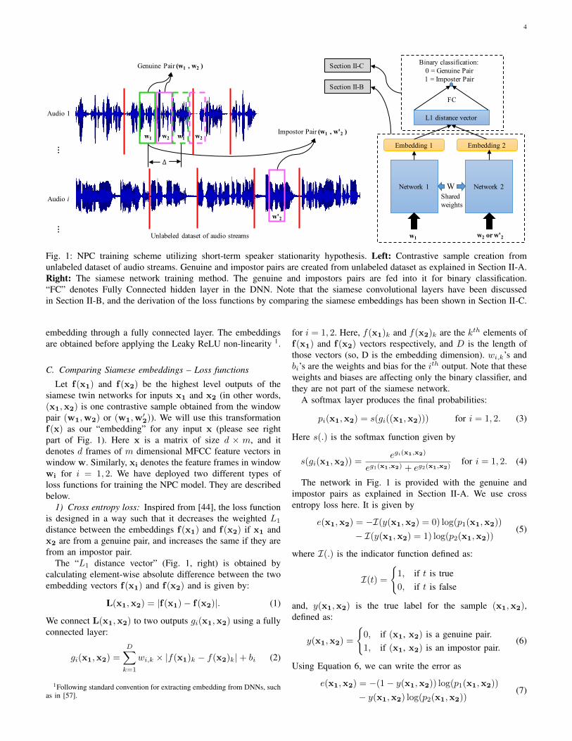
NPC learns to extract speaker characteristics in a contrastiveway i.e. by distinguishing between different speakers. Duringtraining phase, it possesses no information about the actualspeaker identities, but only learns whether two input audiochunks are generated from the same speaker or not. Weprovide the NPC model two kinds of samples [41]. Thefirst kind consists of pairs of speech segments that comefrom the same speaker, called genuine pairs. The secondtype consists of speech segments from two different speakers,called impostor pairs. This approach has been used in the pastfor numerous applications [41], [42], [44], but all of themneeded labeled datasets. The challenge is how we can createsuch samples if we do not have labeled acoustic data. Weexploit the characteristics of speaker-turntaking that result inshort-term speaker stationarity [40]. The hypothesis of short-term speaker stationarity is based on the notion that givena long observation of human interaction, the probability offast speaker changes will be at the tails of the distribution.In short: it is very unlikely to have extremely fast speakerchanges (for example every 1 second). So, if we take pairsof consecutive short segments from such a long audio stream,most of the pairs will contain two audio segments from thesame speaker (genuine pairs). There will be definitely somepairs containing segments from two different speakers, butnumber of such pairs will probably be small compared to thetotal number of genuine pairs. To find the impostor pairs, wechoose two random segments from two different audio streamsin our unsupervised dataset. Again, intuitively the probabilityof finding the same speaker in an impostor pair is relativelylower than the probability of getting two different speakersin it, provided a sufficiently large unsupervised dataset. Forexample, sampling two random YouTube videos, the likelihoodof getting the same speaker in both is very low.

The left part of Fig. 1 shows this contrastive sample creationprocess. Audio stream 1 and audio stream i (for any i between2 to N , where N is the number of audio streams in thedataset) are shown here. Assume the vertical red lines denote(unknown) speaker change points. (w1,w2) is a window pairwhere each of the two windows has d feature frames. Thiswindow pair is moved over the audio streams with a shift of∆ to get the genuine pairs. For every w1, we randomly pick

a window w′2 of same length from a different audio stream toget an impostor pair. All these samples are then fed into thesiamese DNN network for binary classification of whether aninput pair is genuine or impostor.

A siamese neural network (please see right part of Fig. 1),first introduced for signature verification [45], consists of twoidentical twin networks with shared weights that are joined atthe top by some energy function [41], [42], [44]. Generally,the siamese networks are provided with two inputs and trainedby minimizing the energy function which is a predefinedmetric between the highest level feature transformations ofboth the inputs. The weight sharing ensures similar inputsare transformed into embeddings in close proximity with eachother. The inherent structure of a siamese network enables usto learn similar or dissimilar input pairs with discriminativeenergy functions [41], [42]. Similar to [44], we use L1 distanceloss between the highest level outputs of the siamese twinnetworks for the two inputs.

We will first describe in Section II-B about the CNNthat processes the speech spectrogram to automatically learnfeatures to generate the embeddings. Next, in Section II-C wewill discuss about the top part of the neural network of Fig. 1that involves comparing the two embeddings and deriving thefinal output and error for back-propagation.

B. Siamese Convolutional layers

The amazing effectiveness of CNNs have been well estab-lished in computer vision field [46], [47]. Recently, speech sci-entists are also applying CNNs for different challenging taskslike speech recognition [48], [49], speaker recognition [31],[50], [51], large scale audio classification [52] etc. The generalbenefits of using CNNs can be found in [22] and in theabove papers. In our work, the inspiration to use CNNs comesfrom the need of exploring spectral and temporal contextstogether through 2D convolution over the mel-spectrogramfeatures (please see Section III-D for more information). Thebenefits of such a 2D convolution have also been shown withmore traditional signal processing feature sets such as Gaborfeatures [53].

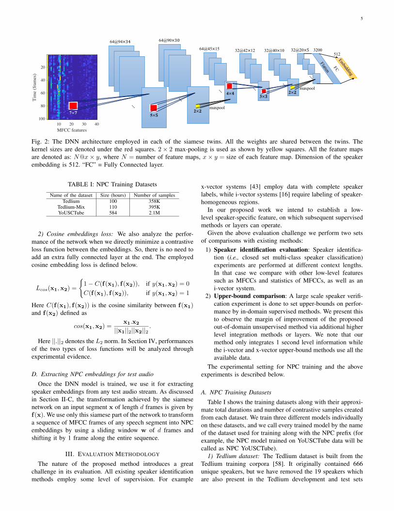
Our siamese network (one of the identical twins), built usingmultiple CNN layers and one dense layer at the highest level, isshown in Fig. 2. We gradually reduce the kernel size from 7×7to 5×5, 4×4, and 3×3. We have used 2×2 max-pooling layersafter every two convolutional layers. The size of stride for allconvolution and max-pooling operations has been chosen tobe 1. We have used Leaky ReLU nonlinearity [54] after everyconvolutional or fully connected layer (omitted from Fig. 2for clearer visualization).

We have applied batch normalization [55] after every layerto reduce the “internal covariance shift” [55] of the network.It helped the network to avoid overfitting and converge fasterwithout the need of using dropout layers [56]. After the lastconvolutional layer, we get 32 feature maps, each of size20 × 5. We flatten these maps to get a 3200 dimensionalvector which is connected to the final 512 dimensional NPC

4

Network 1 Network 2

Embedding 1 Embedding 2

L1 distance vector

W

w1 w2 or w'2

FC

Binary classification:0 = Genuine Pair1 = Imposter Pair

Audio 1

Audio i

……

Genuine Pair (w1 , w2 )

Impostor Pair (w1 , w'2 )w1 w2

w'2

w1 w2

∆

Unlabeled dataset of audio streams

Shared weights

Section II-C

Section II-B

Fig. 1: NPC training scheme utilizing short-term speaker stationarity hypothesis. Left: Contrastive sample creation fromunlabeled dataset of audio streams. Genuine and impostor pairs are created from unlabeled dataset as explained in Section II-A.Right: The siamese network training method. The genuine and impostors pairs are fed into it for binary classification.“FC” denotes Fully Connected hidden layer in the DNN. Note that the siamese convolutional layers have been discussedin Section II-B, and the derivation of the loss functions by comparing the siamese embeddings has been shown in Section II-C.

embedding through a fully connected layer. The embeddingsare obtained before applying the Leaky ReLU non-linearity 1.

C. Comparing Siamese embeddings – Loss functions

Let f(x1) and f(x2) be the highest level outputs of thesiamese twin networks for inputs x1 and x2 (in other words,(x1,x2) is one contrastive sample obtained from the windowpair (w1,w2) or (w1,w

′2)). We will use this transformation

f(x) as our “embedding” for any input x (please see rightpart of Fig. 1). Here x is a matrix of size d × m, and itdenotes d frames of m dimensional MFCC feature vectors inwindow w. Similarly, xi denotes the feature frames in windowwi for i = 1, 2. We have deployed two different types ofloss functions for training the NPC model. They are describedbelow.

1) Cross entropy loss: Inspired from [44], the loss functionis designed in a way such that it decreases the weighted L1

distance between the embeddings f(x1) and f(x2) if x1 andx2 are from a genuine pair, and increases the same if they arefrom an impostor pair.

The “L1 distance vector” (Fig. 1, right) is obtained bycalculating element-wise absolute difference between the twoembedding vectors f(x1) and f(x2) and is given by:

L(x1,x2) = |f(x1)− f(x2)|. (1)

We connect L(x1,x2) to two outputs gi(x1,x2) using a fullyconnected layer:

gi(x1,x2) =

D∑k=1

wi,k × |f(x1)k − f(x2)k|+ bi (2)

1Following standard convention for extracting embedding from DNNs, suchas in [57].

for i = 1, 2. Here, f(x1)k and f(x2)k are the kth elements off(x1) and f(x2) vectors respectively, and D is the length ofthose vectors (so, D is the embedding dimension). wi,k’s andbi’s are the weights and bias for the ith output. Note that theseweights and biases are affecting only the binary classifier, andthey are not part of the siamese network.

A softmax layer produces the final probabilities:

pi(x1,x2) = s(gi((x1,x2))) for i = 1, 2. (3)

Here s(.) is the softmax function given by

s(gi(x1,x2)) =egi(x1,x2)

eg1(x1,x2) + eg2(x1,x2)for i = 1, 2. (4)

The network in Fig. 1 is provided with the genuine andimpostor pairs as explained in Section II-A. We use crossentropy loss here. It is given by

e(x1,x2) = −I(y(x1,x2) = 0) log(p1(x1,x2))

− I(y(x1,x2) = 1) log(p2(x1,x2))(5)

where I(.) is the indicator function defined as:

I(t) =

{1, if t is true0, if t is false

and, y(x1,x2) is the true label for the sample (x1,x2),defined as:

y(x1,x2) =

{0, if (x1, x2) is a genuine pair.1, if (x1, x2) is an impostor pair.

(6)

Using Equation 6, we can write the error as

e(x1,x2) = −(1− y(x1,x2)) log(p1(x1,x2))

− y(x1,x2) log(p2(x1,x2))(7)

5

64@94×3464@45×15

64@90×30

32@42×12 32@40×10 32@20×5

5×𝟓

maxpool2×𝟐

4×𝟒3×𝟑

2×𝟐maxpool

3200512

10 20 30 40MFCC features

20

40

60

80

100

Tim

e (fr

ames

)

7×𝟕

Fig. 2: The DNN architecture employed in each of the siamese twins. All the weights are shared between the twins. Thekernel sizes are denoted under the red squares. 2× 2 max-pooling is used as shown by yellow squares. All the feature mapsare denoted as: N@x× y, where N = number of feature maps, x× y = size of each feature map. Dimension of the speakerembedding is 512. “FC” = Fully Connected layer.

TABLE I: NPC Training Datasets

Name of the dataset Size (hours) Number of samplesTedlium 100 358K

Tedlium-Mix 110 395KYoUSCTube 584 2.1M

2) Cosine embeddings loss: We also analyze the perfor-mance of the network when we directly minimize a contrastiveloss function between the embeddings. So, there is no need toadd an extra fully connected layer at the end. The employedcosine embedding loss is defined below.

Lcos(x1,x2) =

{1− C(f(x1), f(x2)), if y(x1,x2) = 0

C(f(x1), f(x2)), if y(x1,x2) = 1

Here C(f(x1), f(x2)) is the cosine similarity between f(x1)and f(x2) defined as

cos(x1,x2) =x1.x2

||x1||2||x2||2.

Here ||.||2 denotes the L2 norm. In Section IV, performancesof the two types of loss functions will be analyzed throughexperimental evidence.

D. Extracting NPC embeddings for test audio

Once the DNN model is trained, we use it for extractingspeaker embeddings from any test audio stream. As discussedin Section II-C, the transformation achieved by the siamesenetwork on an input segment x of length d frames is given byf(x). We use only this siamese part of the network to transforma sequence of MFCC frames of any speech segment into NPCembeddings by using a sliding window w of d frames andshifting it by 1 frame along the entire sequence.

III. EVALUATION METHODOLOGY

The nature of the proposed method introduces a greatchallenge in its evaluation. All existing speaker identificationmethods employ some level of supervision. For example

x-vector systems [43] employ data with complete speakerlabels, while i-vector systems [16] require labeling of speaker-homogeneous regions.

In our proposed work we intend to establish a low-level speaker-specific feature, on which subsequent supervisedmethods or layers can operate.

Given the above evaluation challenge we perform two setsof comparisons with existing methods:

1) Speaker identification evaluation: Speaker identifica-tion (i.e., closed set multi-class speaker classification)experiments are performed at different context lengths.In that case we compare with other low-level featuressuch as MFCCs and statistics of MFCCs, as well as ani-vector system.

2) Upper-bound comparison: A large scale speaker verifi-cation experiment is done to set upper-bounds on perfor-mance by in-domain supervised methods. We present thisto observe the margin of improvement of the proposedout-of-domain unsupervised method via additional higherlevel integration methods or layers. We note that ourmethod only integrates 1 second level information whilethe i-vector and x-vector upper-bound methods use all theavailable data.

The experimental setting for NPC training and the aboveexperiments is described below.

A. NPC Training Datasets

Table I shows the training datasets along with their approxi-mate total durations and number of contrastive samples createdfrom each dataset. We train three different models individuallyon these datasets, and we call every trained model by the nameof the dataset used for training along with the NPC prefix (forexample, the NPC model trained on YoUSCTube data will becalled as NPC YoUSCTube).

1) Tedlium dataset: The Tedlium dataset is built from theTedlium training corpora [58]. It originally contained 666unique speakers, but we have removed the 19 speakers whichare also present in the Tedlium development and test sets

6

(since the Tedlium dataset was originally developed for speechrecognition purposes, it has speaker overlap between trainand dev/test sets). The contrastive samples created from theTedlium dataset are less noisy (compared to the case forYoUSCTube data as will be discussed next), because most ofthe audio streams in the Tedlium data are from a single speakertalking in the same environment for long (although there issome noise, for example, speech of the audience, clappingetc.).

The reason for employing this dataset is two-fold: First, themodel trained on the Tedlium data will provide a comparisonwith the models trained on the Tedlium-Mix and YoUSCTubedatasets for a validation of the short-term speaker stationarityhypothesis. Second, since the test set of the speaker identifi-cation experiment will be from the Tedlium test data, this willhelp demonstrate the difference in performance for in-domainand out-of-domain evaluation.

2) Tedlium-Mix dataset: The Tedlium-Mix dataset is cre-ated mainly to validate the short-term speaker stationarityhypothesis (please see Section IV-B). We create the Tedlium-Mix dataset by creating artificial dialogs through randomlyconcatenating utterances. Tedlium is annotated, so we knowthe utterance boundaries. We thus simulate a dialog that hasa random speaker every other utterance of the main speaker.For every audio stream, we reject half of the total utterances,and between every two utterances we concatenate a randomlychosen utterance from a randomly chosen speaker (i.e. S, R1,S, R2, S, R3, . . . where S’s are the utterances of the mainspeaker and Ri (for i = 1, 2, 3, . . . ) is a random utterancefrom a randomly chosen speaker i.e. a random utterance fromanother Ted recording). In this way we create the Tedlium-Mix dataset having a speaker change after every utterance forevery audio stream. It also has almost the same size as theTedlium dataset.

3) YoUSCTube dataset: A large amount of various typesof audio data has been collected from YouTube to createthe YoUSCTube dataset. We have chosen YouTube for thispurpose because of virtually unlimited supply of data fromdiverse environments. The dataset has multilingual data includ-ing English, Spanish, Hindi and Telugu from heterogeneousacoustic conditions like monologues, multi-speaker conversa-tions, movie clips with background music and noise, outdoordiscussions etc.

4) Validation data: The Tedlium development set (8 uniquespeakers) has been used as validation data for all trainingcases. We used the utterance start and end time stamps and thespeaker IDs provided in the transcripts of the Tedlium datasetto create the validation set so that it does not have any noisylabels.

B. Data for speaker identification experiment

The Tedlium test set (11 unique speakers from 11 differentTed recordings) has been employed for the speaker identifi-cation experiment. Similar to the development dataset, it hasstart and end time of every utterance for every speaker aswell as the speaker IDs. We have extracted the utterancesfrom every speaker, and all utterances of a particular speaker

0 5 10 15 20 25 30 35 40

Number of epochs

75

80

85

90

95

100

Bin

ary

clas

sifi

catio

n ac

cura

cy (

%)

90.1990.4892.16

Train accuracy for NPC Tedlium Validation accuracy for NPC Tedlium Train accuracy for NPC Tedlium-Mix Validation accuracy for NPC Tedlium-Mix Train accuracy for NPC YoUSCTube Validation accuracy for NPC YoUSCTube

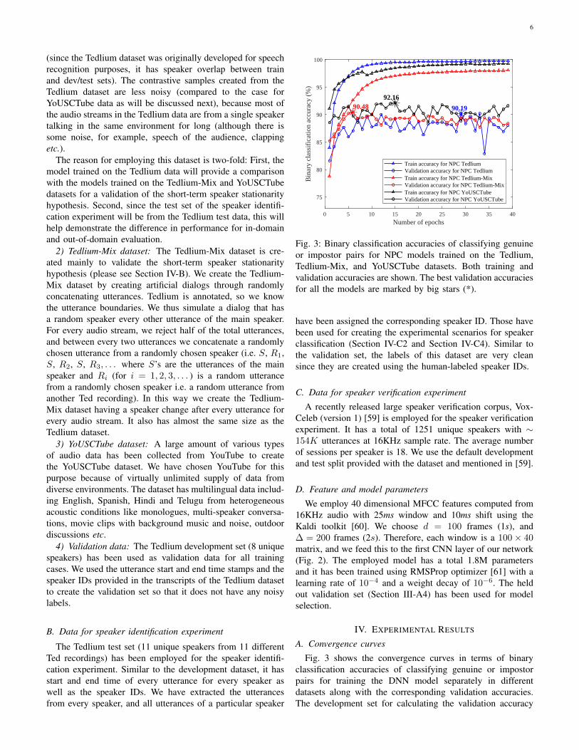
Fig. 3: Binary classification accuracies of classifying genuineor impostor pairs for NPC models trained on the Tedlium,Tedlium-Mix, and YoUSCTube datasets. Both training andvalidation accuracies are shown. The best validation accuraciesfor all the models are marked by big stars (*).

have been assigned the corresponding speaker ID. Those havebeen used for creating the experimental scenarios for speakerclassification (Section IV-C2 and Section IV-C4). Similar tothe validation set, the labels of this dataset are very cleansince they are created using the human-labeled speaker IDs.

C. Data for speaker verification experiment

A recently released large speaker verification corpus, Vox-Celeb (version 1) [59] is employed for the speaker verificationexperiment. It has a total of 1251 unique speakers with ∼154K utterances at 16KHz sample rate. The average numberof sessions per speaker is 18. We use the default developmentand test split provided with the dataset and mentioned in [59].

D. Feature and model parameters

We employ 40 dimensional MFCC features computed from16KHz audio with 25ms window and 10ms shift using theKaldi toolkit [60]. We choose d = 100 frames (1s), and∆ = 200 frames (2s). Therefore, each window is a 100× 40matrix, and we feed this to the first CNN layer of our network(Fig. 2). The employed model has a total 1.8M parametersand it has been trained using RMSProp optimizer [61] with alearning rate of 10−4 and a weight decay of 10−6. The heldout validation set (Section III-A4) has been used for modelselection.

IV. EXPERIMENTAL RESULTS

A. Convergence curves

Fig. 3 shows the convergence curves in terms of binaryclassification accuracies of classifying genuine or impostorpairs for training the DNN model separately in differentdatasets along with the corresponding validation accuracies.The development set for calculating the validation accuracy

7

is same for all the training sets and it doesn’t contain anynoisy samples. In contrast, our training set is noisy sinceit’s unsupervised and based on the short-term stationarity inassigning same/different class speaker pairs.

We can see from Fig. 3 that NPC Tedlium reaches almost100% training accuracy, but NPC Tedlium-Mix converges ata lower training accuracy as expected. This is due to thelarger portion of noisy samples present in the Tedlium-Mixdataset that arise from the artificially introduced fast speakerchanges and the simultaneous hypothesis of short-term speakerstationarity2. However this doesn’t hurt the validation accuracyon the development set, which is both distinct from training setand correctly labeled: we obtain 90.19% and 90.48% for NPCTedlium and NPC Tedlium-Mix trained-models respectively.We believe this is because the model is correctly learning tonot label some of the assumed same-speaker pairs as same-speaker when there is a speaker change that we introducedvia our mixing, due to the large amounts of correct data thatcompensate for the smaller-amount of mislabeled pairs.

The NPC YoUSCTube model reaches much better trainingaccuracy than the NPC Tedlium-Mix model even with fewerepochs. This points to both increased robustness due to theincreased data variability and also that speaker-changes inreal dialogs are not as fast as we simulated in the Tedlium-Mix dataset. It is interesting to see that the NPC YoUSCTubemodel achieves a little better validation accuracy (92.16%)than the other two models even when the training dataset hadno explicit domain overlap with the validation data. We think,this is because of the huge size (approximately 6 times largerin size than the Tedlium dataset) and widely varying types ofacoustic environments of the YoUSCTube dataset.

B. Validation of the short-term speaker stationarity hypothesis

Here we analyze the validation accuracies obtained by theNPC models trained separately on the Tedlium and Tedlium-Mix datasets. From Fig. 3 it is quite clear that both mod-els could achieve similar validation accuracies, although theTedlium-Mix dataset has audio streams containing speakerchanges at every utterance and the Tedlium dataset containsmostly single-speaker audio streams. The reason is that eventhough there are frequent speaker turns in the Tedlium-Mixdataset, the short length of context (d = 100 frames =1s) chosen to learn the speaker characteristics ensures thatthe total number of correct same-speaker pairs dominatethe falsely-labeled same-speaker pairs. Therefore the suddenspeaker changes are of little impact and do not deteriorate theperformance of neural network on the development set. Thisresult validates the short-term speaker stationarity hypothesis.

C. Experiments: Speaker identification evaluation1) Frame-level Embedding visualization: Visualization of

high dimensional data is vital in many scenarios because it

2The corpus is created by mixing turns. This means that there are 54, 778speaker change points in the 115 hours of audio. However in this case weassumed that there are no speaker changes in consecutive frames. If the changepoints were uniformly distributed then that would result in an upper-boundof 87%.

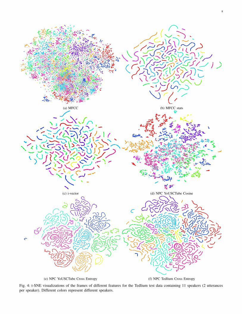
can reveal the inherent structure of the data points. For speakercharacteristics learning, visualizing the employed features canmanifest the clusters formed around different speakers andthus demonstrate the efficacy of the features. We use t-SNEvisualization [62] for this purpose. We compare the followingfeatures (the terms in boldface show the names we will useto call the features).

1) MFCC: Raw MFCC features.2) MFCC stats: This is generated by moving a sliding

window of 1s along the raw MFCC features with a shiftof 1 frame (10ms) and taking the statistics (mean andstandard deviation in the window) to produce a newfeature stream. This is done for a fair comparison ofMFCC and the embeddings (since the embeddings aregenerated using 1s context).

3) NPC YoUSCTube Cross Entropy: Embeddings ex-tracted with NPC YoUSCTube model using cross entropyloss.

4) NPC Tedlium Cross Entropy: Embeddings extractedwith NPC Tedlium model using cross entropy loss.

5) NPC YoUSCTube Cosine: Embeddings extracted withNPC YoUSCTube model using cosine embedding loss.

6) i-vector: 400 dimensional i-vectors extracted indepen-dently every 1s using a sliding window with 10ms shift.The i-vector system (Kaldi VoxCeleb v1 recipe) wastrained on the VoxCeleb dataset [59] (16 KHz audio). Itis not possible to train an i-vector system on YoUSCTubesince it contains no labels on speaker-homogeneous re-gions.

Fig. 4 shows the 2 dimensional t-SNE visualizations of theframes (at 10ms resolution) of the above features extractedfrom the Tedlium test dataset containing 11 unique speakers.For better visualization of the data, we chose only 2 utterancesfrom every speaker, and the feature frames from a total of 22utterances become our input dataset for the t-SNE algorithm.From Fig. 4 we can see that the raw MFCC features arevery noisy, but the inherent smoothing applied to computeMFCC stats features help the features of the same speaker tocome closer. However we notice that although some same-speaker features cluster in lines, these lines are far apart inthe space, which denotes that the MFCC features captureadditional information. For example we see that the speakerdenoted with Green occupies both the very left and very rightparts of the t-SNE space.

The i-vector plot looks similar to the MFCC stats anddoes not cluster the speakers very well. This is consistentwith existing literature [21] that showed that i-vectors do notperform well for short utterances especially when the trainingutterances are comparatively longer. In Section IV-C4, we willsee that the utterance-level i-vectors perform much better forspeaker classification.

The NPC YoUSCTube Cosine embeddings underperformthe cross entropy-based methods possibly because of poorerconvergence as we observed during training. They are alsonoisier than MFCC stats and i-vectors, indicating that even alittle change in the input (just 10ms of extra audio) perturbsthe embedding space, which might not be desirable.

8

(a) MFCC (b) MFCC stats

(c) i-vector (d) NPC YoUSCTube Cosine

(e) NPC YoUSCTube Cross Entropy (f) NPC Tedlium Cross Entropy

Fig. 4: t-SNE visualizations of the frames of different features for the Tedlium test data containing 11 speakers (2 utterancesper speaker). Different colors represent different speakers.

9

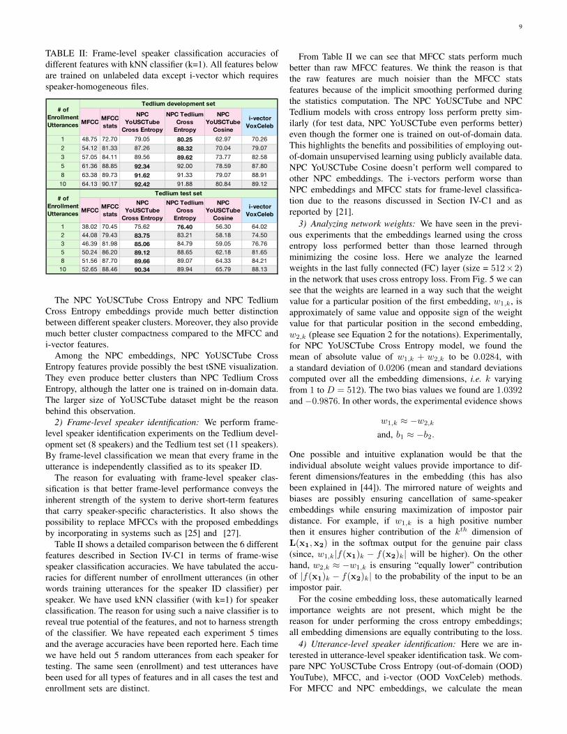
TABLE II: Frame-level speaker classification accuracies ofdifferent features with kNN classifier (k=1). All features beloware trained on unlabeled data except i-vector which requiresspeaker-homogeneous files.

MFCC MFCC stats

NPC YoUSCTube

Cross Entropy

NPC Tedlium Cross

Entropy

NPC YoUSCTube

Cosine

i-vector VoxCeleb

1 48.75 72.70 79.05 80.25 62.97 70.262 54.12 81.33 87.26 88.32 70.04 79.073 57.05 84.11 89.56 89.62 73.77 82.585 61.36 88.85 92.34 92.00 78.59 87.808 63.38 89.73 91.62 91.33 79.07 88.9110 64.13 90.17 92.42 91.88 80.84 89.12

MFCC MFCC stats

NPC YoUSCTube

Cross Entropy

NPC Tedlium Cross

Entropy

NPC YoUSCTube

Cosine

i-vector VoxCeleb

1 38.02 70.45 75.62 76.40 56.30 64.022 44.08 79.43 83.75 83.21 58.18 74.503 46.39 81.98 85.06 84.79 59.05 76.765 50.24 86.20 89.12 88.65 62.18 81.658 51.56 87.70 89.66 89.07 64.33 84.2110 52.65 88.46 90.34 89.94 65.79 88.13

# of Enrollment Utterances

Tedlium test set

Tedlium development set

# of Enrollment Utterances

The NPC YoUSCTube Cross Entropy and NPC TedliumCross Entropy embeddings provide much better distinctionbetween different speaker clusters. Moreover, they also providemuch better cluster compactness compared to the MFCC andi-vector features.

Among the NPC embeddings, NPC YoUSCTube CrossEntropy features provide possibly the best tSNE visualization.They even produce better clusters than NPC Tedlium CrossEntropy, although the latter one is trained on in-domain data.The larger size of YoUSCTube dataset might be the reasonbehind this observation.

2) Frame-level speaker identification: We perform frame-level speaker identification experiments on the Tedlium devel-opment set (8 speakers) and the Tedlium test set (11 speakers).By frame-level classification we mean that every frame in theutterance is independently classified as to its speaker ID.

The reason for evaluating with frame-level speaker clas-sification is that better frame-level performance conveys theinherent strength of the system to derive short-term featuresthat carry speaker-specific characteristics. It also shows thepossibility to replace MFCCs with the proposed embeddingsby incorporating in systems such as [25] and [27].

Table II shows a detailed comparison between the 6 differentfeatures described in Section IV-C1 in terms of frame-wisespeaker classification accuracies. We have tabulated the accu-racies for different number of enrollment utterances (in otherwords training utterances for the speaker ID classifier) perspeaker. We have used kNN classifier (with k=1) for speakerclassification. The reason for using such a naive classifier is toreveal true potential of the features, and not to harness strengthof the classifier. We have repeated each experiment 5 timesand the average accuracies have been reported here. Each timewe have held out 5 random utterances from each speaker fortesting. The same seen (enrollment) and test utterances havebeen used for all types of features and in all cases the test andenrollment sets are distinct.

From Table II we can see that MFCC stats perform muchbetter than raw MFCC features. We think the reason is thatthe raw features are much noisier than the MFCC statsfeatures because of the implicit smoothing performed duringthe statistics computation. The NPC YoUSCTube and NPCTedlium models with cross entropy loss perform pretty sim-ilarly (for test data, NPC YoUSCTube even performs better)even though the former one is trained on out-of-domain data.This highlights the benefits and possibilities of employing out-of-domain unsupervised learning using publicly available data.NPC YoUSCTube Cosine doesn’t perform well compared toother NPC embeddings. The i-vectors perform worse thanNPC embeddings and MFCC stats for frame-level classifica-tion due to the reasons discussed in Section IV-C1 and asreported by [21].

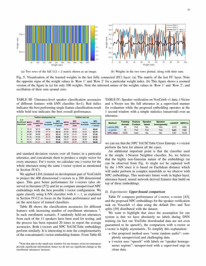
3) Analyzing network weights: We have seen in the previ-ous experiments that the embeddings learned using the crossentropy loss performed better than those learned throughminimizing the cosine loss. Here we analyze the learnedweights in the last fully connected (FC) layer (size = 512×2)in the network that uses cross entropy loss. From Fig. 5 we cansee that the weights are learned in a way such that the weightvalue for a particular position of the first embedding, w1,k, isapproximately of same value and opposite sign of the weightvalue for that particular position in the second embedding,w2,k (please see Equation 2 for the notations). Experimentally,for NPC YoUSCTube Cross Entropy model, we found themean of absolute value of w1,k + w2,k to be 0.0284, witha standard deviation of 0.0206 (mean and standard deviationscomputed over all the embedding dimensions, i.e. k varyingfrom 1 to D = 512). The two bias values we found are 1.0392and −0.9876. In other words, the experimental evidence shows

w1,k ≈ −w2,k

and, b1 ≈ −b2.

One possible and intuitive explanation would be that theindividual absolute weight values provide importance to dif-ferent dimensions/features in the embedding (this has alsobeen explained in [44]). The mirrored nature of weights andbiases are possibly ensuring cancellation of same-speakerembeddings while ensuring maximization of impostor pairdistance. For example, if w1,k is a high positive numberthen it ensures higher contribution of the kth dimension ofL(x1,x2) in the softmax output for the genuine pair class(since, w1,k|f(x1)k − f(x2)k| will be higher). On the otherhand, w2,k ≈ −w1,k is ensuring “equally lower” contributionof |f(x1)k − f(x2)k| to the probability of the input to be animpostor pair.

For the cosine embedding loss, these automatically learnedimportance weights are not present, which might be thereason for under performing the cross entropy embeddings;all embedding dimensions are equally contributing to the loss.

4) Utterance-level speaker identification: Here we are in-terested in utterance-level speaker identification task. We com-pare NPC YoUSCTube Cross Entropy (out-of-domain (OOD)YouTube), MFCC, and i-vector (OOD VoxCeleb) methods.For MFCC and NPC embeddings, we calculate the mean

10

50 100 150 200 250 300 350 400 450 500Weight index

Row 1

Row 2

Wei

ght v

alue

-0.4

-0.3

-0.2

-0.1

0

0.1

0.2

0.3

0.4

(a) Two rows of the full 512× 2 matrix shown as an image.

0 10 20 30 40 50 60 70 80 90 100Weight index

-0.3

-0.2

-0.1

0

0.1

0.2

0.3

0.4

Wei

ght v

alue

Row 1Row 2Row 1 + Row 2

(b) Weights in the two rows plotted, along with their sum.

Fig. 5: Visualization of the learned weights in the last fully connected (FC) layer: (a) The matrix of the last FC layer. Notethe opposite signs of the weight values in ‘Row 1’ and ‘Row 2’ for a particular weight index. (b) This figure shows a zoomedversion of the figure in (a) for only 100 weights. Note the mirrored nature of the weights values in ‘Row 1’ and ‘Row 2’, andoscillation of their sum around zero.

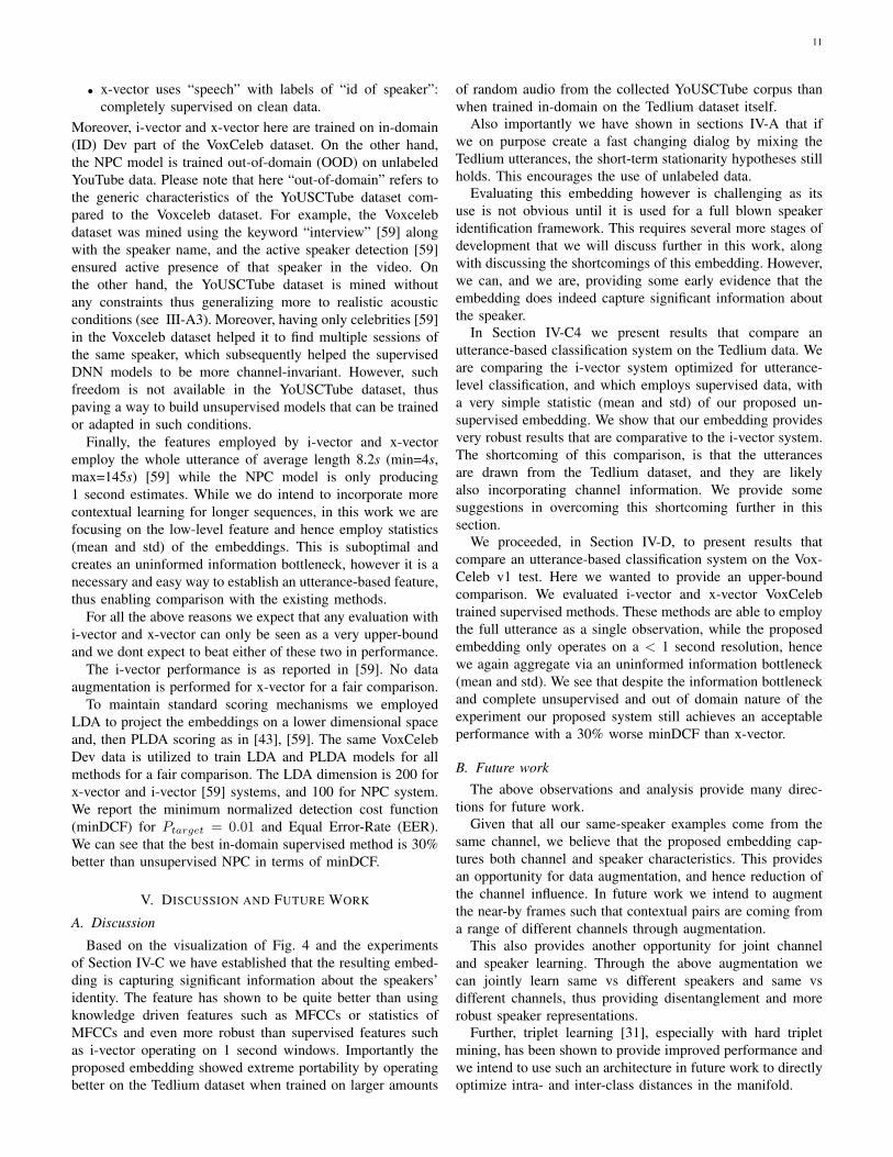
TABLE III: Utterance-level speaker classification accuraciesof different features with kNN classifier (k=1). Red italicsindicates the best performing single feature classification resultwhile bold text indicates the best overall performance.

MFCC stats

NPC YoUSCTube

stats

i-vector VoxCeleb

NPC YoUSCTube

+ i-vector

MFCC stats

NPC YoUSCTube

stats

i-vector VoxCeleb

NPC YoUSCTube

+ i-vector

1 75.12 82.12 86.38 85.62 80.00 83.27 85.00 86.822 83.00 87.88 91.75 92.12 87.64 92.36 92.82 95.733 84.88 89.88 93.12 93.12 92.18 95.45 94.82 97.095 91.25 94.50 95.25 95.88 92.09 95.36 93.91 95.458 92.12 95.00 96.62 97.25 95.27 97.36 95.82 97.3610 92.50 95.25 95.12 96.50 96.54 98.00 96.73 98.09

# of Enrollment Utterances

Tedlium test setTedlium development set

and standard deviation vectors over all frames in a particularutterance, and concatenate them to produce a single vector forevery utterance. For i-vector, we calculate one i-vector for thewhole utterance using the same i-vector system as mentionedin Section IV-C1.

We applied LDA (trained on development part of VoxCeleb)to project the 400 dimensional i-vectors to a 200 dimensionalspace. This gave better performance for i-vectors (also ob-served in literature [57]) and let us compare unsupervised NPCembeddings with the best possible i-vector configuration. Weagain classify using k-NN classifier with k = 1, as explainedin Section IV-C2 to focus on the feature performance and noton the next-layer of trained classifiers.

Table III shows the classification accuracies for differentfeatures with increasing number of enrollment utterances 3.In each enrollment scenario, 5 randomly held-out utterancesfrom each of the 11 speakers have been used for testing, andthe process has been repeated 20 times to report the averageaccuracies. Both i-vectors and NPC YoUSCTube embeddingsperform similarly. It is interesting to note the complementarityof the concatenated i-vector-embedding feature. From Table III

3Note that due to the small-size window for our feature, even two utterancesprovide significant information; hence we do not see significant change as theenrollment utterances increase.

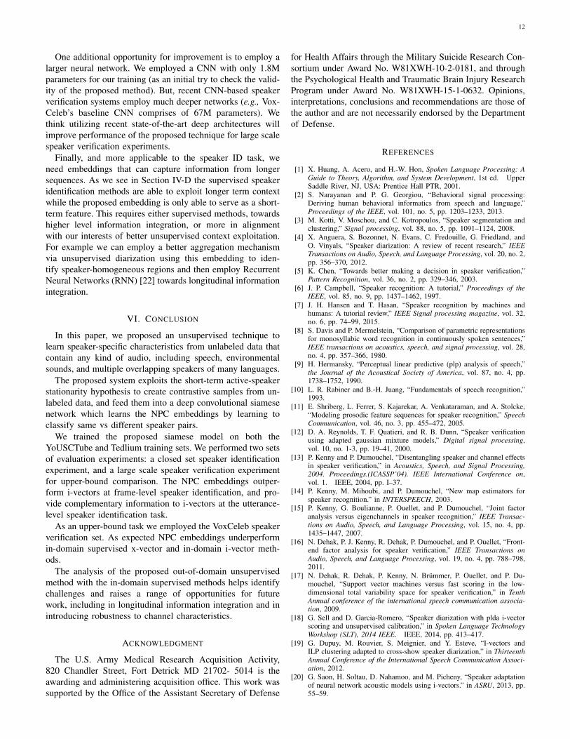
TABLE IV: Speaker verification on VoxCeleb v1 data. i-Vectorand x-Vector use the full utterance in a supervised mannerfor evaluation while the proposed embedding operates at the1 second window with a simple statistics (mean+std) over anutterance.

Method Training domain

Feature Context

Speaker labels

Speaker homogeneity minDCF EER(%)

i-vector [59] ID Full No Yes 0.73 8.80x-vector ID Full Full Yes 0.61 7.21

NPC stats OOD 1sec No No 0.87 15.54

we can see that the NPC YoUSCTube Cross Entropy + i-vectorperform the best for almost all the cases.

An additional important point is that the classifier usedis the simple 1-Nearest Neighbor classifier. So, we believethat the highly non-Gaussian nature of the embeddings (ascan be observed from Fig. 4) might not be captured wellby the 1-NN since it is based on Euclidean distance whichwill under perform in complex manifolds as we observe withNPC embeddings. This motivates future work in higher-layer,utterance-based, neural network-derived features that build ontop of these embeddings.

D. Experiments: Upper-bound comparisonTable IV compares performance of i-vector, x-vector [43],

and the proposed NPC embeddings for the speaker verificationtask on Voxceleb v1 data using the default Dev and Testsplits [59] distributed with the dataset.

We want to highlight that since the assumption for oursystem is that we have absolutely no labels during DNNtraining (in fact our YouTube downloaded data are not evenguaranteed to be speech!), the comparison with x-vector ori-vector is highly asymmetric. To simplify this explanation:• Our proposed method uses “some random audio”: com-

pletely unsupervised and challenging data.• i-vector uses “speech” with labels on “speaker homoge-

neous regions”: unsupervised with a supervised step onclean data.

11

• x-vector uses “speech” with labels of “id of speaker”:completely supervised on clean data.

Moreover, i-vector and x-vector here are trained on in-domain(ID) Dev part of the VoxCeleb dataset. On the other hand,the NPC model is trained out-of-domain (OOD) on unlabeledYouTube data. Please note that here “out-of-domain” refers tothe generic characteristics of the YoUSCTube dataset com-pared to the Voxceleb dataset. For example, the Voxcelebdataset was mined using the keyword “interview” [59] alongwith the speaker name, and the active speaker detection [59]ensured active presence of that speaker in the video. Onthe other hand, the YoUSCTube dataset is mined withoutany constraints thus generalizing more to realistic acousticconditions (see III-A3). Moreover, having only celebrities [59]in the Voxceleb dataset helped it to find multiple sessions ofthe same speaker, which subsequently helped the supervisedDNN models to be more channel-invariant. However, suchfreedom is not available in the YoUSCTube dataset, thuspaving a way to build unsupervised models that can be trainedor adapted in such conditions.

Finally, the features employed by i-vector and x-vectoremploy the whole utterance of average length 8.2s (min=4s,max=145s) [59] while the NPC model is only producing1 second estimates. While we do intend to incorporate morecontextual learning for longer sequences, in this work we arefocusing on the low-level feature and hence employ statistics(mean and std) of the embeddings. This is suboptimal andcreates an uninformed information bottleneck, however it is anecessary and easy way to establish an utterance-based feature,thus enabling comparison with the existing methods.

For all the above reasons we expect that any evaluation withi-vector and x-vector can only be seen as a very upper-boundand we dont expect to beat either of these two in performance.

The i-vector performance is as reported in [59]. No dataaugmentation is performed for x-vector for a fair comparison.

To maintain standard scoring mechanisms we employedLDA to project the embeddings on a lower dimensional spaceand, then PLDA scoring as in [43], [59]. The same VoxCelebDev data is utilized to train LDA and PLDA models for allmethods for a fair comparison. The LDA dimension is 200 forx-vector and i-vector [59] systems, and 100 for NPC system.We report the minimum normalized detection cost function(minDCF) for Ptarget = 0.01 and Equal Error-Rate (EER).We can see that the best in-domain supervised method is 30%better than unsupervised NPC in terms of minDCF.

V. DISCUSSION AND FUTURE WORK

A. Discussion

Based on the visualization of Fig. 4 and the experimentsof Section IV-C we have established that the resulting embed-ding is capturing significant information about the speakers’identity. The feature has shown to be quite better than usingknowledge driven features such as MFCCs or statistics ofMFCCs and even more robust than supervised features suchas i-vector operating on 1 second windows. Importantly theproposed embedding showed extreme portability by operatingbetter on the Tedlium dataset when trained on larger amounts

of random audio from the collected YoUSCTube corpus thanwhen trained in-domain on the Tedlium dataset itself.

Also importantly we have shown in sections IV-A that ifwe on purpose create a fast changing dialog by mixing theTedlium utterances, the short-term stationarity hypotheses stillholds. This encourages the use of unlabeled data.

Evaluating this embedding however is challenging as itsuse is not obvious until it is used for a full blown speakeridentification framework. This requires several more stages ofdevelopment that we will discuss further in this work, alongwith discussing the shortcomings of this embedding. However,we can, and we are, providing some early evidence that theembedding does indeed capture significant information aboutthe speaker.

In Section IV-C4 we present results that compare anutterance-based classification system on the Tedlium data. Weare comparing the i-vector system optimized for utterance-level classification, and which employs supervised data, witha very simple statistic (mean and std) of our proposed un-supervised embedding. We show that our embedding providesvery robust results that are comparative to the i-vector system.The shortcoming of this comparison, is that the utterancesare drawn from the Tedlium dataset, and they are likelyalso incorporating channel information. We provide somesuggestions in overcoming this shortcoming further in thissection.

We proceeded, in Section IV-D, to present results thatcompare an utterance-based classification system on the Vox-Celeb v1 test. Here we wanted to provide an upper-boundcomparison. We evaluated i-vector and x-vector VoxCelebtrained supervised methods. These methods are able to employthe full utterance as a single observation, while the proposedembedding only operates on a < 1 second resolution, hencewe again aggregate via an uninformed information bottleneck(mean and std). We see that despite the information bottleneckand complete unsupervised and out of domain nature of theexperiment our proposed system still achieves an acceptableperformance with a 30% worse minDCF than x-vector.

B. Future workThe above observations and analysis provide many direc-

tions for future work.Given that all our same-speaker examples come from the

same channel, we believe that the proposed embedding cap-tures both channel and speaker characteristics. This providesan opportunity for data augmentation, and hence reduction ofthe channel influence. In future work we intend to augmentthe near-by frames such that contextual pairs are coming froma range of different channels through augmentation.

This also provides another opportunity for joint channeland speaker learning. Through the above augmentation wecan jointly learn same vs different speakers and same vsdifferent channels, thus providing disentanglement and morerobust speaker representations.

Further, triplet learning [31], especially with hard tripletmining, has been shown to provide improved performance andwe intend to use such an architecture in future work to directlyoptimize intra- and inter-class distances in the manifold.

12

One additional opportunity for improvement is to employ alarger neural network. We employed a CNN with only 1.8Mparameters for our training (as an initial try to check the valid-ity of the proposed method). But, recent CNN-based speakerverification systems employ much deeper networks (e.g., Vox-Celeb’s baseline CNN comprises of 67M parameters). Wethink utilizing recent state-of-the-art deep architectures willimprove performance of the proposed technique for large scalespeaker verification experiments.

Finally, and more applicable to the speaker ID task, weneed embeddings that can capture information from longersequences. As we see in Section IV-D the supervised speakeridentification methods are able to exploit longer term contextwhile the proposed embedding is only able to serve as a short-term feature. This requires either supervised methods, towardshigher level information integration, or more in alignmentwith our interests of better unsupervised context exploitation.For example we can employ a better aggregation mechanismvia unsupervised diarization using this embedding to iden-tify speaker-homogeneous regions and then employ RecurrentNeural Networks (RNN) [22] towards longitudinal informationintegration.

VI. CONCLUSION

In this paper, we proposed an unsupervised technique tolearn speaker-specific characteristics from unlabeled data thatcontain any kind of audio, including speech, environmentalsounds, and multiple overlapping speakers of many languages.

The proposed system exploits the short-term active-speakerstationarity hypothesis to create contrastive samples from un-labeled data, and feed them into a deep convolutional siamesenetwork which learns the NPC embeddings by learning toclassify same vs different speaker pairs.

We trained the proposed siamese model on both theYoUSCTube and Tedlium training sets. We performed two setsof evaluation experiments: a closed set speaker identificationexperiment, and a large scale speaker verification experimentfor upper-bound comparison. The NPC embeddings outper-form i-vectors at frame-level speaker identification, and pro-vide complementary information to i-vectors at the utterance-level speaker identification task.

As an upper-bound task we employed the VoxCeleb speakerverification set. As expected NPC embeddings underperformin-domain supervised x-vector and in-domain i-vector meth-ods.

The analysis of the proposed out-of-domain unsupervisedmethod with the in-domain supervised methods helps identifychallenges and raises a range of opportunities for futurework, including in longitudinal information integration and inintroducing robustness to channel characteristics.

ACKNOWLEDGMENT

The U.S. Army Medical Research Acquisition Activity,820 Chandler Street, Fort Detrick MD 21702- 5014 is theawarding and administering acquisition office. This work wassupported by the Office of the Assistant Secretary of Defense

for Health Affairs through the Military Suicide Research Con-sortium under Award No. W81XWH-10-2-0181, and throughthe Psychological Health and Traumatic Brain Injury ResearchProgram under Award No. W81XWH-15-1-0632. Opinions,interpretations, conclusions and recommendations are those ofthe author and are not necessarily endorsed by the Departmentof Defense.

REFERENCES

[1] X. Huang, A. Acero, and H.-W. Hon, Spoken Language Processing: AGuide to Theory, Algorithm, and System Development, 1st ed. UpperSaddle River, NJ, USA: Prentice Hall PTR, 2001.

[2] S. Narayanan and P. G. Georgiou, “Behavioral signal processing:Deriving human behavioral informatics from speech and language,”Proceedings of the IEEE, vol. 101, no. 5, pp. 1203–1233, 2013.

[3] M. Kotti, V. Moschou, and C. Kotropoulos, “Speaker segmentation andclustering,” Signal processing, vol. 88, no. 5, pp. 1091–1124, 2008.

[4] X. Anguera, S. Bozonnet, N. Evans, C. Fredouille, G. Friedland, andO. Vinyals, “Speaker diarization: A review of recent research,” IEEETransactions on Audio, Speech, and Language Processing, vol. 20, no. 2,pp. 356–370, 2012.

[5] K. Chen, “Towards better making a decision in speaker verification,”Pattern Recognition, vol. 36, no. 2, pp. 329–346, 2003.

[6] J. P. Campbell, “Speaker recognition: A tutorial,” Proceedings of theIEEE, vol. 85, no. 9, pp. 1437–1462, 1997.

[7] J. H. Hansen and T. Hasan, “Speaker recognition by machines andhumans: A tutorial review,” IEEE Signal processing magazine, vol. 32,no. 6, pp. 74–99, 2015.

[8] S. Davis and P. Mermelstein, “Comparison of parametric representationsfor monosyllabic word recognition in continuously spoken sentences,”IEEE transactions on acoustics, speech, and signal processing, vol. 28,no. 4, pp. 357–366, 1980.

[9] H. Hermansky, “Perceptual linear predictive (plp) analysis of speech,”the Journal of the Acoustical Society of America, vol. 87, no. 4, pp.1738–1752, 1990.

[10] L. R. Rabiner and B.-H. Juang, “Fundamentals of speech recognition,”1993.

[11] E. Shriberg, L. Ferrer, S. Kajarekar, A. Venkataraman, and A. Stolcke,“Modeling prosodic feature sequences for speaker recognition,” SpeechCommunication, vol. 46, no. 3, pp. 455–472, 2005.

[12] D. A. Reynolds, T. F. Quatieri, and R. B. Dunn, “Speaker verificationusing adapted gaussian mixture models,” Digital signal processing,vol. 10, no. 1-3, pp. 19–41, 2000.

[13] P. Kenny and P. Dumouchel, “Disentangling speaker and channel effectsin speaker verification,” in Acoustics, Speech, and Signal Processing,2004. Proceedings.(ICASSP’04). IEEE International Conference on,vol. 1. IEEE, 2004, pp. I–37.

[14] P. Kenny, M. Mihoubi, and P. Dumouchel, “New map estimators forspeaker recognition.” in INTERSPEECH, 2003.

[15] P. Kenny, G. Boulianne, P. Ouellet, and P. Dumouchel, “Joint factoranalysis versus eigenchannels in speaker recognition,” IEEE Transac-tions on Audio, Speech, and Language Processing, vol. 15, no. 4, pp.1435–1447, 2007.

[16] N. Dehak, P. J. Kenny, R. Dehak, P. Dumouchel, and P. Ouellet, “Front-end factor analysis for speaker verification,” IEEE Transactions onAudio, Speech, and Language Processing, vol. 19, no. 4, pp. 788–798,2011.

[17] N. Dehak, R. Dehak, P. Kenny, N. Brummer, P. Ouellet, and P. Du-mouchel, “Support vector machines versus fast scoring in the low-dimensional total variability space for speaker verification,” in TenthAnnual conference of the international speech communication associa-tion, 2009.

[18] G. Sell and D. Garcia-Romero, “Speaker diarization with plda i-vectorscoring and unsupervised calibration,” in Spoken Language TechnologyWorkshop (SLT), 2014 IEEE. IEEE, 2014, pp. 413–417.

[19] G. Dupuy, M. Rouvier, S. Meignier, and Y. Esteve, “I-vectors andILP clustering adapted to cross-show speaker diarization,” in ThirteenthAnnual Conference of the International Speech Communication Associ-ation, 2012.

[20] G. Saon, H. Soltau, D. Nahamoo, and M. Picheny, “Speaker adaptationof neural network acoustic models using i-vectors.” in ASRU, 2013, pp.55–59.

13

[21] A. Kanagasundaram, R. Vogt, D. B. Dean, S. Sridharan, and M. W.Mason, “I-vector based speaker recognition on short utterances,” inProceedings of the 12th Annual Conference of the International SpeechCommunication Association. International Speech CommunicationAssociation (ISCA), 2011, pp. 2341–2344.

[22] I. Goodfellow, Y. Bengio, and A. Courville, Deep Learning. MIT Press,2016, http://www.deeplearningbook.org.

[23] M. Rouvier, P.-M. Bousquet, and B. Favre, “Speaker diarization throughspeaker embeddings,” in Signal Processing Conference (EUSIPCO),2015 23rd European. IEEE, 2015, pp. 2082–2086.

[24] G. E. Hinton and R. R. Salakhutdinov, “Reducing the dimensionality ofdata with neural networks,” science, vol. 313, no. 5786, pp. 504–507,2006.

[25] T. Yamada, L. Wang, and A. Kai, “Improvement of distant-talkingspeaker identification using bottleneck features of dnn.” in Interspeech,2013, pp. 3661–3664.

[26] E. Variani, X. Lei, E. McDermott, I. L. Moreno, and J. Gonzalez-Dominguez, “Deep neural networks for small footprint text-dependentspeaker verification,” in Acoustics, Speech and Signal Processing(ICASSP), 2014 IEEE International Conference on. IEEE, 2014, pp.4052–4056.

[27] S. H. Ghalehjegh and R. C. Rose, “Deep bottleneck features for i-vector based text-independent speaker verification,” in Automatic SpeechRecognition and Understanding (ASRU), 2015 IEEE Workshop on.IEEE, 2015, pp. 555–560.

[28] K. Chen and A. Salman, “Learning speaker-specific characteristics witha deep neural architecture,” IEEE Transactions on Neural Networks,vol. 22, no. 11, pp. 1744–1756, 2011.

[29] ——, “Extracting speaker-specific information with a regularizedsiamese deep network,” in Advances in Neural Information ProcessingSystems, 2011, pp. 298–306.

[30] D. Snyder, P. Ghahremani, D. Povey, D. Garcia-Romero, Y. Carmiel, andS. Khudanpur, “Deep neural network-based speaker embeddings for end-to-end speaker verification,” in Spoken Language Technology Workshop(SLT), 2016 IEEE. IEEE, 2016, pp. 165–170.

[31] C. Li, X. Ma, B. Jiang, X. Li, X. Zhang, X. Liu, Y. Cao, A. Kannan,and Z. Zhu, “Deep speaker: an end-to-end neural speaker embeddingsystem,” arXiv preprint arXiv:1705.02304, 2017.

[32] S. J. Pan, Q. Yang et al., “A survey on transfer learning,” IEEETransactions on knowledge and data engineering, vol. 22, no. 10, pp.1345–1359, 2010.

[33] M. M. Saleem and J. H. Hansen, “A discriminative unsupervised methodfor speaker recognition using deep learning,” in Machine Learning forSignal Processing (MLSP), 2016 IEEE 26th International Workshop on.IEEE, 2016, pp. 1–5.

[34] X.-L. Zhang, “Multilayer bootstrap network for unsupervised speakerrecognition,” arXiv preprint arXiv:1509.06095, 2015.

[35] I. Lapidot, H. Guterman, and A. Cohen, “Unsupervised speaker recogni-tion based on competition between self-organizing maps,” IEEE Trans-actions on Neural Networks, vol. 13, no. 4, pp. 877–887, 2002.

[36] H. Lee, P. Pham, Y. Largman, and A. Y. Ng, “Unsupervised featurelearning for audio classification using convolutional deep belief net-works,” in Advances in neural information processing systems, 2009,pp. 1096–1104.

[37] J. S. Garofolo, L. F. Lamel, W. M. Fisher, J. G. Fiscus,D. S. Pallett, N. L. Dahlgren, and V. Zue, “Timit acoustic-phonetic continuous speech corpus ldc93s1,” 1993. [Online]. Available:https://catalog.ldc.upenn.edu/LDC93S1

[38] D. O’Shaughnessy, “Linear predictive coding,” IEEE potentials, vol. 7,no. 1, pp. 29–32, 1988.

[39] H. Li, B. Baucom, and P. Georgiou, “Unsupervised latent behavior mani-fold learning from acoustic features: Audio2behavior,” in Proceedings ofIEEE International Conference on Audio, Speech and Signal Processing(ICASSP), New Orleans, Louisiana, March 2017.

[40] A. Jati and P. Georgiou, “Speaker2vec: Unsupervised learning andadaptation of a speaker manifold using deep neural networks with anevaluation on speaker segmentation,” in Proceedings of Interspeech,August 2017.

[41] S. Chopra, R. Hadsell, and Y. LeCun, “Learning a similarity metricdiscriminatively, with application to face verification,” in ComputerVision and Pattern Recognition, 2005. CVPR 2005. IEEE ComputerSociety Conference on, vol. 1. IEEE, 2005, pp. 539–546.

[42] R. Hadsell, S. Chopra, and Y. LeCun, “Dimensionality reduction bylearning an invariant mapping,” in Computer vision and pattern recog-nition, 2006 IEEE computer society conference on, vol. 2. IEEE, 2006,pp. 1735–1742.

[43] D. Snyder, D. Garcia-Romero, G. Sell, D. Povey, and S. Khudanpur, “X-vectors: Robust dnn embeddings for speaker recognition,” Submitted toICASSP, 2018.

[44] G. Koch, R. Zemel, and R. Salakhutdinov, “Siamese neural networks forone-shot image recognition,” in ICML Deep Learning Workshop, vol. 2,2015.

[45] J. Bromley, I. Guyon, Y. LeCun, E. Sackinger, and R. Shah, “Signatureverification using a” siamese” time delay neural network,” in Advancesin Neural Information Processing Systems, 1994, pp. 737–744.

[46] A. Krizhevsky, I. Sutskever, and G. E. Hinton, “Imagenet classificationwith deep convolutional neural networks,” in Advances in neural infor-mation processing systems, 2012, pp. 1097–1105.

[47] K. Simonyan and A. Zisserman, “Very deep convolutional networks forlarge-scale image recognition,” arXiv preprint arXiv:1409.1556, 2014.

[48] O. Abdel-Hamid, A. R. Mohamed, H. Jiang, L. Deng, G. Penn,and D. Yu, “Convolutional neural networks for speech recognition,”IEEE/ACM Transactions on audio, speech, and language processing,vol. 22, no. 10, pp. 1533–1545, 2014.

[49] G. Hinton, L. Deng, D. Yu, G. E. Dahl, A.-r. Mohamed, N. Jaitly,A. Senior, V. Vanhoucke, P. Nguyen, T. N. Sainath et al., “Deep neuralnetworks for acoustic modeling in speech recognition: The shared viewsof four research groups,” IEEE Signal Processing Magazine, vol. 29,no. 6, pp. 82–97, 2012.

[50] M. McLaren, Y. Lei, N. Scheffer, and L. Ferrer, “Application of convo-lutional neural networks to speaker recognition in noisy conditions,” inFifteenth Annual Conference of the International Speech CommunicationAssociation, 2014.

[51] Y. Lukic, C. Vogt, O. Durr, and T. Stadelmann, “Speaker identifica-tion and clustering using convolutional neural networks,” in MachineLearning for Signal Processing (MLSP), 2016 IEEE 26th InternationalWorkshop on. IEEE, 2016, pp. 1–6.

[52] S. Hershey, S. Chaudhuri, D. P. W. Ellis, J. F. Gemmeke, A. Jansen,R. C. Moore, M. Plakal, D. Platt, R. A. Saurous, B. Seybold,M. Slaney, R. J. Weiss, and K. W. Wilson, “CNN architectures forlarge-scale audio classification,” CoRR, vol. abs/1609.09430, 2016.[Online]. Available: http://arxiv.org/abs/1609.09430

[53] S.-Y. Chang and N. Morgan, “Robust cnn-based speech recognition withgabor filter kernels,” in Fifteenth Annual Conference of the InternationalSpeech Communication Association, 2014.

[54] A. L. Maas, A. Y. Hannun, and A. Y. Ng, “Rectifier nonlinearitiesimprove neural network acoustic models,” in Proc. ICML, vol. 30, no. 1,2013.

[55] S. Ioffe and C. Szegedy, “Batch normalization: Accelerating deepnetwork training by reducing internal covariate shift,” in Proceedingsof the 32nd International Conference on Machine Learning, ser.Proceedings of Machine Learning Research, F. Bach and D. Blei, Eds.,vol. 37. Lille, France: PMLR, 07–09 Jul 2015, pp. 448–456. [Online].Available: http://proceedings.mlr.press/v37/ioffe15.html

[56] N. Srivastava, G. E. Hinton, A. Krizhevsky, I. Sutskever, andR. Salakhutdinov, “Dropout: a simple way to prevent neural networksfrom overfitting.” Journal of Machine Learning Research, vol. 15, no. 1,pp. 1929–1958, 2014.

[57] D. Snyder, D. Garcia-Romero, D. Povey, and S. Khudanpur, “Deepneural network embeddings for text-independent speaker verification,”Proc. Interspeech 2017, pp. 999–1003, 2017.

[58] A. Rousseau, P. Deleglise, and Y. Esteve, “Ted-lium: an automaticspeech recognition dedicated corpus.” in LREC, 2012, pp. 125–129.

[59] A. Nagrani, J. S. Chung, and A. Zisserman, “VoxCeleb: a large-scalespeaker identification dataset,” arXiv preprint arXiv:1706.08612, 2017.

[60] D. Povey, A. Ghoshal, G. Boulianne, L. Burget, O. Glembek, N. Goel,M. Hannemann, P. Motlicek, Y. Qian, P. Schwarz, J. Silovsky, G. Stem-mer, and K. Vesely, “The kaldi speech recognition toolkit,” in IEEE 2011Workshop on Automatic Speech Recognition and Understanding. IEEESignal Processing Society, Dec. 2011, iEEE Catalog No.: CFP11SRW-USB.

[61] T. Tieleman and G. Hinton, “Lecture 6.5-RMSProp: Divide the gradientby a running average of its recent magnitude,” COURSERA: Neuralnetworks for machine learning, vol. 4, no. 2, pp. 26–31, 2012.

[62] L. Van Der Maaten and G. Hinton, “Visualizing data using t-SNE,”Journal of Machine Learning Research, vol. 9, no. Nov, pp. 2579–2605,2008.