Information Paper Australian National Accounts ... · interpretation of input-output multipliers. Second, it provides details of the way in which the input-output multiplier tables

Information PaperAustralian National

AccountsIntroduction to

Input-OutputMultipliers

Catalogue No. 5246.0

INFORMATION PAPER:AUSTRALIAN NATIONAL ACCOUNTS: INTRODUCTION TO

INPUT-OUTPUT MULTIPLIERS

W. McLennanAustralian Statistician

AUSTRALIAN BUREAU OF STATISTICS CATALOGUE NO.5246.0

CONTENTS

Paragraph Section Page

Foreword v

1-12 INPUT-OUTPUT TABLES 1

1 Introduction 1

2-9 Structure 1

10-12 Interpreting input-output tables 1

Exercises 6

13-36 MULTIPLIERS 6

13-15 Introduction 6

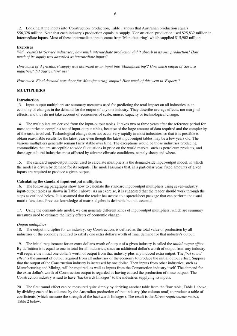
16-34 Calculating the standard input-output multipliers 6

18-30 Output multipliers 6

31-32 Income multipliers 9

33 Employment multipliers 10

34-36 Summary 10

Exercises 10

37 RELATED PUBLICATIONS 10

GLOSSARY OF TERMS 13

Appendix A Technical note 15

Appendix B Illustrative examples 18

Appendix C Underlying assumptions and interpretation of input-output multipliers 24

Answers to exercise questions 25

Order Form for Multipliers tables

INQUIRIES for further information about ABS input-output multipliers, contact Mr Alan Tryde on Canberra(06) 252 6808.for further information about ABS input-output tables, contact Mr Peter Claydon on Canberra(06) 252 6910.for further information about ABS statistics and services, please refer to the back page of thispublication.

iii

FOREWORD

Input-Output tables are part of the Australian national accounts, complementing the quarterly and annual series ofnational income, expenditure and product aggregates. They provide detailed information about the supply anddisposition of commodities in the Australian economy and about the structure of, and inter-relationships between,Australian industries.

Detailed data on supply and use of commodities, inter-industry flows and a range of derived data, such as input-outputmultipliers, are provided for economic planning and analysis, and construction of models for forecasting purposes.The data can also be useful for non-economists seeking a thorough knowledge of relationships in the Australianeconomy.

This publication is intended to serve three main purposes. First, it provides a guide to the construction andinterpretation of input-output multipliers. Second, it provides details of the way in which the input-output multipliertables can be used. Third, it provides a means of answering some of the questions often asked by input-outputpractitioners. These queries tend to arise because of the types of "what if?" analysis for which input-output tablescan be used (for example, what would be the impact on employment of an x% change in output by the chemicalindustry). This type of analysis is really dependent on a knowledge of input-output multipliers and theirshortcomings. Using input-output tables, multipliers can be calculated to provide a simple means of working out theflow on effects of a change in output in an industry on one or more of imports, income, employment or output inindividual industries or in total. The multipliers can show just the 'first-round' effects, or the aggregated effects onceall secondary effects have flowed through the system.

Australian Bureau of StatisticsBelconnen, ACT 2616

W. McLennan Australian Statistician

v

1

INTRODUCTION TO INPUT-OUTPUT MULTIPLIERS

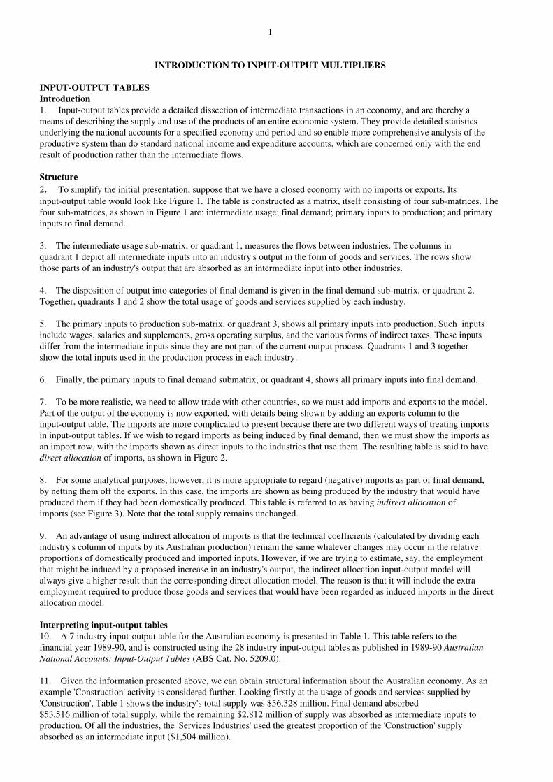
INPUT-OUTPUT TABLESIntroduction1. Input-output tables provide a detailed dissection of intermediate transactions in an economy, and are thereby ameans of describing the supply and use of the products of an entire economic system. They provide detailed statisticsunderlying the national accounts for a specified economy and period and so enable more comprehensive analysis of theproductive system than do standard national income and expenditure accounts, which are concerned only with the endresult of production rather than the intermediate flows.

Structure2. To simplify the initial presentation, suppose that we have a closed economy with no imports or exports. Itsinput-output table would look like Figure 1. The table is constructed as a matrix, itself consisting of four sub-matrices. Thefour sub-matrices, as shown in Figure 1 are: intermediate usage; final demand; primary inputs to production; and primaryinputs to final demand.

3. The intermediate usage sub-matrix, or quadrant 1, measures the flows between industries. The columns inquadrant 1 depict all intermediate inputs into an industry's output in the form of goods and services. The rows showthose parts of an industry's output that are absorbed as an intermediate input into other industries.

4. The disposition of output into categories of final demand is given in the final demand sub-matrix, or quadrant 2.Together, quadrants 1 and 2 show the total usage of goods and services supplied by each industry.

5. The primary inputs to production sub-matrix, or quadrant 3, shows all primary inputs into production. Such inputsinclude wages, salaries and supplements, gross operating surplus, and the various forms of indirect taxes. These inputsdiffer from the intermediate inputs since they are not part of the current output process. Quadrants 1 and 3 togethershow the total inputs used in the production process in each industry.

6. Finally, the primary inputs to final demand submatrix, or quadrant 4, shows all primary inputs into final demand.

7. To be more realistic, we need to allow trade with other countries, so we must add imports and exports to the model.Part of the output of the economy is now exported, with details being shown by adding an exports column to theinput-output table. The imports are more complicated to present because there are two different ways of treating importsin input-output tables. If we wish to regard imports as being induced by final demand, then we must show the imports asan import row, with the imports shown as direct inputs to the industries that use them. The resulting table is said to havedirect allocation of imports, as shown in Figure 2.

8. For some analytical purposes, however, it is more appropriate to regard (negative) imports as part of final demand,by netting them off the exports. In this case, the imports are shown as being produced by the industry that would haveproduced them if they had been domestically produced. This table is referred to as having indirect allocation ofimports (see Figure 3). Note that the total supply remains unchanged.

9. An advantage of using indirect allocation of imports is that the technical coefficients (calculated by dividing eachindustry's column of inputs by its Australian production) remain the same whatever changes may occur in the relativeproportions of domestically produced and imported inputs. However, if we are trying to estimate, say, the employmentthat might be induced by a proposed increase in an industry's output, the indirect allocation input-output model willalways give a higher result than the corresponding direct allocation model. The reason is that it will include the extraemployment required to produce those goods and services that would have been regarded as induced imports in the directallocation model.

Interpreting input-output tables10. A 7 industry input-output table for the Australian economy is presented in Table 1. This table refers to thefinancial year 1989-90, and is constructed using the 28 industry input-output tables as published in 1989-90 AustralianNational Accounts: Input-Output Tables (ABS Cat. No. 5209.0).

11. Given the information presented above, we can obtain structural information about the Australian economy. As anexample 'Construction' activity is considered further. Looking firstly at the usage of goods and services supplied by'Construction', Table 1 shows the industry's total supply was $56,328 million. Final demand absorbed $53,516 million of total supply, while the remaining $2,812 million of supply was absorbed as intermediate inputs toproduction. Of all the industries, the 'Services Industries' used the greatest proportion of the 'Construction' supplyabsorbed as an intermediate input ($1,504 million).

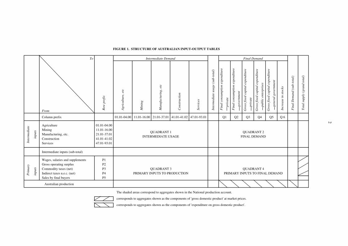
FIGURE 1. STRUCTURE OF AUSTRALIAN INPUT-OUTPUT TABLES

To Intermediate Demand Final Demand

From R

ow p

refi

x

A

gric

ultu

re, e

tc

M

inin

g

M

anuf

actu

ring

, etc

C

onst

ruct

ion

Se

rvic

es

In

term

edia

te u

sage

(su

b-to

tal)

F

inal

con

sum

ptio

n ex

pend

itur

e

pri

vate

F

inal

con

sum

ptio

n ex

pend

itur

e

gov

ernm

ent

Gro

ss fi

xed

capi

tal e

xpen

ditu

re

pri

vate

Gro

ss fi

xed

capi

tal e

xpen

ditu

re

pub

lic

ente

rpri

ses

Gro

ss fi

xed

capi

tal e

xpen

ditu

re

gen

eral

gov

ernm

ent

In

crea

se in

sto

cks

F

inal

Dem

and

(sub

-tot

al)

T

otal

sup

ply

(gra

nd to

tal)

Column prefix 01.01-04.00 11.01-16.00 21.01-37.01 41.01-41.02 47.01-93.01 Q1 Q2 Q3 Q4 Q5 Q 6

Inte

rmed

iate

inpu

ts

Agriculture Mining Manufacturing, etc. Construction Services

01.01-04.00 11.01-16.00 21.01-37.01 41.01-41.02 47.01-93.01

QUADRANT 1 INTERMEDIATE USAGE

QUADRANT 2 FINAL DEMAND

2

Intermediate inputs (sub-total)

Pri

mar

y

inpu

ts

Wages, salaries and supplements Gross operating surplus Commodity taxes (net) Indirect taxes n.e.c. (net)

P1 P2 P3 P4

QUADRANT 3 PRIMARY INPUTS TO PRODUCTION

QUADRANT 4 PRIMARY INPUTS TO FINAL DEMAND

Sales by final buyers P5

Australian production

The shaded areas correspond to aggregates shown in the National production account.

corresponds to aggregates shown as the components of 'gross domestic product' at market prices.

corresponds to aggregates shown as the components of 'expenditure on gross domestic product'.

FIGURE 2. STRUCTURE OF AUSTRALIAN INPUT-OUTPUT TABLESDirect allocation of imports, Basic values, Recording of intra-industry flows


From R

ow p

refi

x

A

gric

ultu

re, e

tc

M

inin

g

M

anuf

actu

ring

, etc

C

onst

ruct

ion

Se

rvic

es

In

term

edia

te u

sage

(su

b-to

tal)

F

inal

con

sum

ptio

n ex

pend

itur

e

pri

vate

F

inal

con

sum

ptio

n ex

pend

itur

e

gov

ernm

ent

Gro

ss fi

xed

capi

tal e

xpen

ditu

re

pri

vate

Gro

ss fi

xed

capi

tal e

xpen

ditu

re

pub

lic

ente

rpri

ses

Gro

ss fi

xed

capi

tal e

xpen

ditu

re

gen

eral

gov

ernm

ent

In

crea

se in

sto

cks

E

xpor

ts o

f goo

ds a

nd s

ervi

ces

F

inal

Dem

and

(sub

-tot

al)

T

otal

sup

ply

(gra

nd to

tal)

Column prefix 01.01-04.00 11.01-16.00 21.01-37.01 41.01-41.02 47.01-93.01 Q1 Q2 Q3 Q4 Q5 Q 6 Q 7

Inte

rmed

iate

inpu

ts


01.01-04.00 11.01-16.00 21.01-37.01 41.01-41.02 47.01-93.01



3


Pri

mar

y

inpu

ts


P1 P2 P3 P4




Imports P6





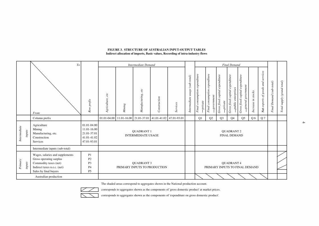
FIGURE 3. STRUCTURE OF AUSTRALIAN INPUT-OUTPUT TABLESIndirect allocation of imports, Basic values, Recording of intra-industry flows


From R

ow p

refi

x

A

gric

ultu

re, e

tc

M

inin

g

M

anuf

actu

ring

, etc

C

onst

ruct

ion

Se

rvic

es

In

term

edia

te u

sage

(su

b-to

tal)

F

inal

con

sum

ptio

n ex

pend

itur

e

pri

vate

F

inal

con

sum

ptio

n ex

pend

itur

e

gov

ernm

ent

Gro

ss fi

xed

capi

tal e

xpen

ditu

re

pri

vate

Gro

ss fi

xed

capi

tal e

xpen

ditu

re

pub

lic

ente

rpri

ses

Gro

ss fi

xed

capi

tal e

xpen

ditu

re

gen

eral

gov

ernm

ent

In

crea

se in

sto

cks

Net

exp

orts

of g

oods

and

ser

vice

s

F

inal

Dem

and

(sub

-tot

al)

T

otal

sup

ply

(gra

nd to

tal)

Column prefix 01.01-04.00 11.01-16.00 21.01-37.01 41.01-41.02 47.01-93.01 Q1 Q2 Q3 Q4 Q5 Q 6 Q 7

Inte

rmed

iate

inpu

ts


01.01-04.00 11.01-16.00 21.01-37.01 41.01-41.02 47.01-93.01



4


Pri

mar

y

inpu

ts


P1 P2 P3 P4








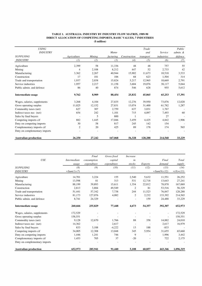
TABLE 1. AUSTRALIA: INDUSTRY BY INDUSTRY FLOW MATRIX, 1989-90DIRECT ALLOCATION OF COMPETING IMPORTS, BASIC VALUES, 7 INDUSTRIES

($ million)

USING Trade Public INDUSTRY Manu- and Service admin. &

SUPPLYING Agriculture Mining facturing Construction transport industries defence INDUSTRY (1) (2) (3) (4) (5) (6) (7)

Agriculture 2,399 58 11,336 48 48 757 55Mining 4 2,108 8,212 447 52 2,733 42Manufacturing 3,362 2,267 40,944 15,902 11,673 10,518 3,533Construction 17 181 106 68 623 1,504 314Trade and transportation 1,937 2,038 15,824 5,217 12,965 10,669 2,791Service industries 1,957 2,217 11,158 3,604 19,076 38,117 5,044Public admin. and defence 86 40 874 546 628 955 5,612

Intermediate usage 9,762 8,909 88,454 25,832 45,065 65,253 17,391

Wages, salaries, supplements 3,268 4,104 27,835 12,276 39,950 73,076 12,020Gross operating surplus 11,025 12,152 27,831 13,074 31,400 61,782 1,287Commodity taxes (net) 627 307 2,759 637 3,031 1,767 -Indirect taxes nec (net) 654 242 1,101 715 4,097 7,493 60Sales by final buyers - 5 800 1 - 27 -Competing imports cif 882 1,445 17,046 3,459 4,425 4,842 1,906Duty on competing imports 30 58 817 245 142 154 -Complementary imports cif 2 20 425 89 178 174 565Duty on complementary imports - - - - - - -

Australian production 26,250 27,242 167,068 56,328 128,288 214,568 33,229

Final Gross fixed Increase

USE Intermediate consumption capital in Final Total

usage expenditure expenditure stocks Exports demand supply

SUPPLYING (8) (9) (10) (11) (12) (13) (14)

INDUSTRY =Sum(1)-(7) =Sum(9)-(12) =(8)+(13)

Agriculture 14,701 3,224 155 2,540 5,632 11,551 26,252Mining 13,598 81 313 531 12,718 13,643 27,241Manufacturing 88,199 39,893 15,611 1,354 22,012 78,870 167,069Construction 2,813 3,884 49,549 2 81 53,516 56,329Trade and transportation 51,441 57,342 7,738 244 11,523 76,847 128,288Service industries 81,173 127,076 4,082 2 2,232 133,392 214,565Public admin. and defence 8,741 24,329 - - 159 24,488 33,229

Intermediate usage 260,666 255,829 77,448 4,673 54,357 392,307 652,973

Wages, salaries, supplements 172,529 - - - - - 172,529Gross operating surplus 158,551 - - - - - 158,551Commodity taxes (net) 9,128 12,670 1,766 88 358 14,882 24,010Indirect taxes nec (net) 14,362 - 2,617 - - 2,617 16,979Sales by final buyers 833 3,188 -4,222 13 188 -833 -Competing imports cif 34,005 12,308 13,048 345 5,954 31,655 65,660Duty on competing imports 1,446 1,241 746 9 - 1,996 3,442Complementary imports cif 1,453 705 37 -20 - 722 2,175Duty on complementary imports - - - - - - -

Australian production 652,973 285,941 91,440 5,108 60,857 443,346 1,096,319

6

12. Looking at the inputs into 'Construction' production, Table 1 shows that Australian production equals $56,328 million. Note that each industry's production equals its supply. 'Construction' production used $25,832 million inintermediate inputs. Most of these intermediate inputs came from 'Manufacturing', which supplied $15,902 million.

ExercisesWith regards to 'Service industries', how much intermediate production did it absorb in its own production? Howmuch of its supply was absorbed as intermediate inputs?

How much of 'Agriculture' supply was absorbed as an input into 'Manufacturing'? How much output of 'Serviceindustries' did 'Agriculture' use?

How much 'Final demand' was there for 'Manufacturing' output? How much of this went to 'Exports'?

MULTIPLIERS

Introduction13. Input-output multipliers are summary measures used for predicting the total impact on all industries in aneconomy of changes in the demand for the output of any one industry. They describe average effects, not marginaleffects, and thus do not take account of economies of scale, unused capacity or technological change.

14. The multipliers are derived from the input-output tables. It takes two or three years after the reference period formost countries to compile a set of input-output tables, because of the large amount of data required and the complexityof the tasks involved. Technological change does not occur very rapidly in most industries, so that it is possible toobtain reasonable results for the latest year even though the latest input-output tables may be a few years old. Thevarious multipliers generally remain fairly stable over time. The exceptions would be those industries producingcommodities that are susceptible to wide fluctuations in price on the world market, such as petroleum products, andthose agricultural industries most affected by adverse climatic conditions, namely sheep and wheat.

15. The standard input-output model used to calculate multipliers is the demand-side input-output model, in whichthe model is driven by demand for its outputs. The model assumes that, in a particular year, fixed amounts of giveninputs are required to produce a given output.

Calculating the standard input-output multipliers16. The following paragraphs show how to calculate the standard input-output multipliers using seven-industryinput-output tables as shown in Table 1 above. As an exercise, it is suggested that the reader should work through thesteps as outlined below. It is assumed that the reader has access to a spreadsheet package that can perform the usualmatrix functions. Previous knowledge of matrix algebra is desirable but not essential.

17. Using the demand-side model, we can generate different kinds of input-output multipliers, which are summarymeasures used to estimate the likely effects of economic change.

Output multipliers18. The output multiplier for an industry, say Construction, is defined as the total value of production by allindustries of the economy required to satisfy one extra dollar's worth of final demand for that industry's output.

19. The initial requirement for an extra dollar's worth of output of a given industry is called the initial output effect.By definition it is equal to one in total for all industries, since an additional dollar's worth of output from any industrywill require the initial one dollar's worth of output from that industry plus any induced extra output. The first roundeffect is the amount of output required from all industries of the economy to produce the initial output effect. Supposethat the output of the Construction industry is increased by one dollar. Then inputs from other industries, such asManufacturing and Mining, will be required, as well as inputs from the Construction industry itself. The demand forthe extra dollar's worth of Construction output is regarded as having caused the production of these outputs. TheConstruction industry is said to have "backwards linkages" to the industries supplying its inputs.

20. The first round effect can be measured quite simply by deriving another table from the flow table, Table 1 above,by dividing each of its columns by the Australian production of that industry (the column total) to produce a table ofcoefficients (which measure the strength of the backwards linkages). The result is the Direct requirements matrix,Table 2 below.

7

TABLE 2. AUSTRALIA: DIRECT REQUIREMENTS COEFFICIENTS, 1989-90 DIRECT ALLOCATION OF COMPETING IMPORTS, BASIC VALUES, 7 INDUSTRIES

USING Trade Public

INDUSTRY Manu- and Service admin. &SUPPLYING Agriculture Mining facturing Construction transport industries defence

INDUSTRY (1) (2) (3) (4) (5) (6) (7)

Agriculture 9.14 0.21 6.79 0.09 0.04 0.35 0.17Mining 0.02 7.74 4.92 0.79 0.04 1.27 0.13Manufacturing 12.81 8.32 24.51 28.23 9.10 4.90 10.63Construction 0.06 0.66 0.06 0.12 0.49 0.70 0.94Trade and transportation 7.38 7.48 9.47 9.26 10.11 4.97 8.40Service industries 7.46 8.14 6.68 6.40 14.87 17.76 15.18Public admin. and defence 0.33 0.15 0.52 0.97 0.49 0.44 16.89

Intermediate usage 37.19 32.70 52.94 45.86 35.13 30.41 52.34

Wages, salaries, supplements 12.45 15.06 16.66 21.79 31.14 34.06 36.17Gross operating surplus 42.00 44.61 16.66 23.21 24.48 28.79 3.87Commodity taxes (net) 2.39 1.13 1.65 1.13 2.36 0.82 —Indirect taxes nec (net) 2.49 0.89 0.66 1.27 3.19 3.49 0.18Sales by final buyers — — 0.48 — — — —Complementary imports cif — 0.07 0.25 0.16 0.14 0.08 1.70Duty on complementary imports — — — — — — —Competing imports cif 3.36 5.30 10.20 6.14 3.45 2.26 5.73Duty on competing imports 0.11 0.21 0.49 0.43 0.11 0.07 —

Australian production 100.00 100.00 100.00 100.00 100.00 100.00 100.00

Final Gross fixed Increase USE Intermediate consumption capital in Final Total

usage expenditure expenditure stocks Exports demand supply

SUPPLYING (8) (9) (10) (11) (12) (13) (14)INDUSTRY =Sum(1)-(7) =Sum(9)-(12) =(8)+(13)

Agriculture 2.25 1.13 0.17 49.72 9.25 2.61 2.39Mining 2.08 0.03 0.34 10.40 20.90 3.08 2.48Manufacturing 13.51 13.95 17.07 26.51 36.17 17.79 15.24Construction 0.43 1.36 54.19 0.04 0.13 12.07 5.14Trade and transportation 7.88 20.05 8.46 4.79 18.93 17.33 11.70Service industries 12.43 44.44 4.46 0.04 3.67 30.09 19.57Public admin. and defence 1.34 8.51 — — 0.26 5.52 3.03

Intermediate usage 39.92 89.47 84.70 91.49 89.32 88.49 59.56

Wages, salaries, supplements 26.42 — — — — — 15.74Gross operating surplus 24.28 — — — — — 14.46Commodity taxes nec (net) 1.40 4.43 1.93 1.73 0.59 3.36 2.19Indirect taxes nec (net) 2.20 — 2.86 — — 0.59 1.55Sales by final buyers 0.13 1.12 -4.62 0.26 0.31 -0.19 —Complementary imports cif 0.22 0.25 — -0.39 — 0.16 0.20Duty on complementary imports — — — — — — —Competing imports cif 5.21 4.30 14.27 6.75 9.78 7.14 5.99Duty on competing imports 0.22 0.43 0.82 0.18 — 0.45 0.31

Australian production 100.00 100.00 100.00 100.00 100.00 100.00 100.00

8

21. The coefficients in a given industry's column of this table show the amount of extra output required from eachindustry to produce an extra dollar's worth of output from that industry. For example, to produce an extra dollar's worthof output from the Construction industry, the Manufacturing industry must have produced an extra $0.28 worth ofoutput, the Trade and transportation industry must have produced an extra $0.09 worth, and so on.

22. Similarly, the extra output from the Manufacturing industry will induce extra output from all industries of theeconomy and, in turn, these will induce extra output, and so on. The combined effects of the initial effects plus all ofthe production induced rounds of extra output are called the simple multipliers.

23. To calculate the simple multipliers, we take the first seven rows and columns of the Direct Requirements Tableand form the A matrix (also referred to as the intermediate usage matrix or the first quadrant of the DirectRequirements matrix). We set up a 7x7 matrix I with all its diagonal elements equal to 1 and all its other elementsequal to zero and calculate a new matrix (I - A). Then we call the matrix inversion function (available on spreadsheetsprograms) to calculate the Leontief inverse (I - A) -1. We then form the column totals. These are the required simplemultipliers. Appendix A provides more detail about this process.

24. Example: All output multipliers are presented in Table 5 in this paper. The simple multiplier for Mining showsthat $1.53 of extra output from the Australian economy is induced by an additional output of $1.00 in the Miningindustry. In other words, to produce an additional unit of output in 'Mining', aside from Mining's additional unit ofoutput, the economy's output must increase by an additional $0.33 in order to provide inputs to 'Mining', and in turn toincrease by $0.21 to provide inputs to the suppliers to 'Mining'. The effects encompassed by the simple multiplier arethe initial effects ($1.00), the first round effects ($0.33) and the industrial support effects ($0.21).

25. It can be shown that this procedure is mathematically equivalent to calculating the effects of all of the rounds ofinduced production and adding them to the initial effects. Since we already know the initial effects and the first roundeffects, we can now calculate the industrial-support effects, the effects of the second and subsequent rounds of inducedproduction, as follows:

industrial support effects = simple multiplier - initial effects

- first round effects.

We can also calculate the production induced effects:

production induced effects = first round effects + industrial support effects.

26. The household sector receives wages for work done in the production process and spends some or all of thiswage income on goods and services. The wages are shown in the Wages, salaries and supplements row andconsumption by households is shown in the Private final consumption expenditure column of the flow matrix. ThePrivate final consumption expenditure can be regarded as generating the production of goods and services by theindustries of the economy. This induced production of extra goods and services is referred to as the consumption-induced effects. A new set of multipliers can be calculated taking into account the initial effects, the productioninduced effects and the consumption induced effects. These are called the total multipliers.

27. The total multipliers are calculated by defining an 8x8 matrix (the B matrix), which is formed by adding to thepreviously defined A matrix the Wages, salaries and supplements row and the Private final consumption expenditurecolumn of the Direct Requirements Coefficients matrix (Table 2). In effect, we are adding a "household" industry tothe economy.

28. In calculating the simple multipliers, we effectively assume that the spending of households takes place outsidethe model and there is no feedback between the household sector and the other sectors. We are said to be using an openmodel. However, in calculating the total multipliers, we do allow feedback to occur, and the model is said to be closedwith respect to households. The open and closed models are shown in Figure 4.

29. The total multipliers are calculated by taking the Leontief inverse of the B matrix, (I - B) -1 (note that this timewe require an 8x8 I matrix). Then we form a new matrix, B*, from the first seven rows and columns of theLeontief inverse of the B matrix and add up the column totals. These are the total multipliers. The consumptioninduced effects can then be calculated:

9

9

consumption induced effects = total multiplier - simple multiplier.

30. Example: The total output multiplier for 'Construction' was calculated to be $2.73. This implies that $2.73 inadditional output is required from all industries to satisfy an increased demand of $1.00 in the construction sector, aswell as to satisfy the additional demand generated by the increased wages, salaries and supplements resulting from allincreased output. This multiplier incorporates all the effects of the simple multiplier, plus the consumption effects.

FIGURE 4. OPEN AND CLOSED MODELS

MATRIX USED TO CONSTRUCT THE OPEN MODEL DIRECTALLOCATION MATRIX

(7 x 7)

QUADRANT 1

INTERMDIATE USAGE

MATRIX USED TO CONSTRUCT THE CLOSED MODELDIRECT ALLOCATION MATRIX

(8 x 8)

QUADRANT 1

INTERMEDIATE USAGE

WAGES, SALARIES AND SU PPLEMENTS

Income multipliers31. The income multiplier for a given industry is defined as the total value of income from wages, salaries andsupplements required to satisfy a dollar's worth of final demand for the output of that industry. We have alreadycalculated the household coefficients in the Wages, salaries and supplements row of the Direct Requirements matrix(Table 2), and these are the initial household income effects. For simplicity, we can refer to them as the vector h.

32. The remaining income multipliers can be calculated using the matrix multiplication function of a spreadsheet package as follows:

first round income effects = h * Asimple income multipliers = h * (I - A) -1

total income multipliers = h * B*.

Note that * denotes matrix multiplication (which is not the same as ordinary multiplication).

The remaining income multipliers can then be calculated in the same way as the corresponding output multipliers.

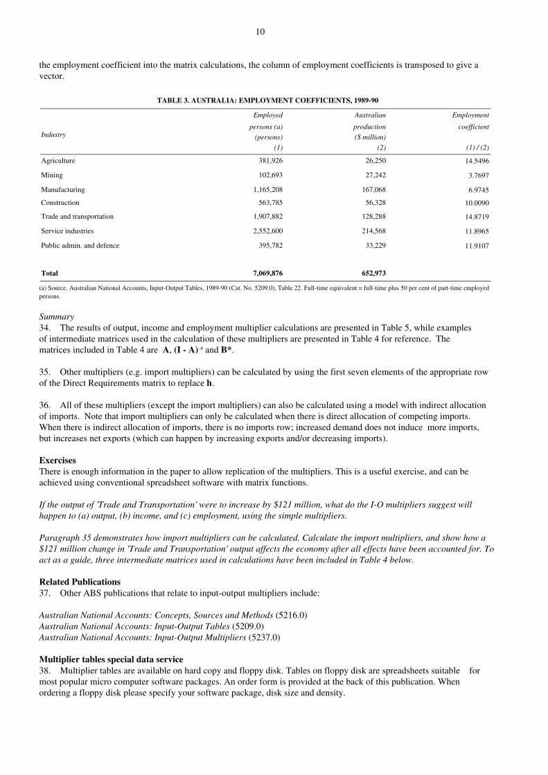
Employment multipliers33. Employment multipliers can be obtained by using the row vector of employment coefficients, e, instead of h. Theemployment coefficients are calculated by dividing the number of employed persons in a given industry by the level ofproduction generated by that industry. This calculation, as well as the raw data involved in this step, is included inTable 3. In this table, the employment multipliers relate to an extra $1 million of output. To incorporate

FINA

L

CO

NSU

MPT

ION

E

XPE

ND

ITU

RE

10

the employment coefficient into the matrix calculations, the column of employment coefficients is transposed to give avector.

TABLE 3. AUSTRALIA: EMPLOYMENT COEFFICIENTS, 1989-90

Industry

Employed

persons (a)

(persons)

(1)

Australian

production

($ million)

(2)

Employment

coefficient

(1) / (2)

Agriculture 381,926 26,250 14.5496

Mining 102,693 27,242 3.7697

Manufacturing 1,165,208 167,068 6.9745

Construction 563,785 56,328 10.0090

Trade and transportation 1,907,882 128,288 14.8719

Service industries 2,552,600 214,568 11.8965

Public admin. and defence 395,782 33,229 11.9107

Total 7,069,876 652,973

(a) Source. Australian National Accounts, Input-Output Tables, 1989-90 (Cat. No. 5209.0), Table 22. Full-time equivalent = full-time plus 50 per cent of part-time employedpersons.

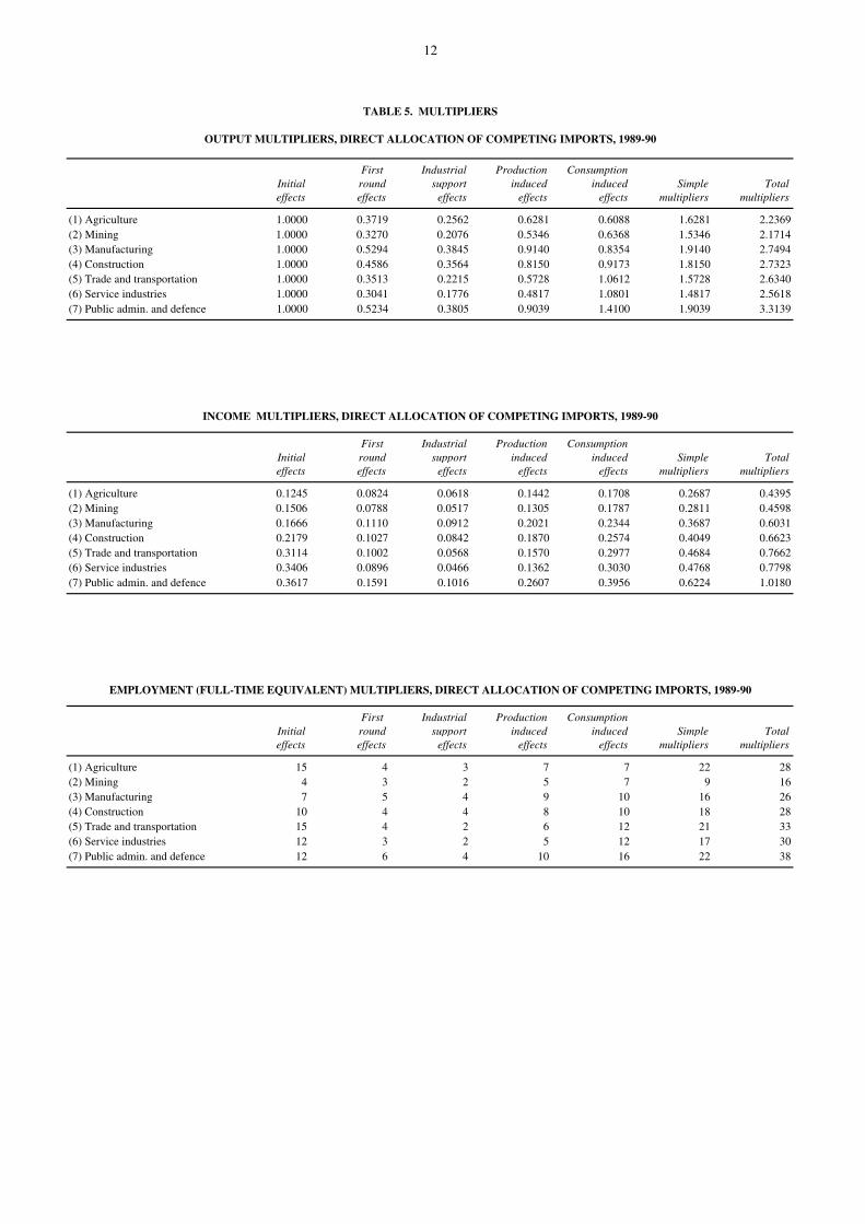
Summary34. The results of output, income and employment multiplier calculations are presented in Table 5, while examplesof intermediate matrices used in the calculation of these multipliers are presented in Table 4 for reference. The matrices included in Table 4 are A, (I - A) -1 and B*. 35. Other multipliers (e.g. import multipliers) can be calculated by using the first seven elements of the appropriate rowof the Direct Requirements matrix to replace h.

36. All of these multipliers (except the import multipliers) can also be calculated using a model with indirect allocationof imports. Note that import multipliers can only be calculated when there is direct allocation of competing imports.When there is indirect allocation of imports, there is no imports row; increased demand does not induce more imports,but increases net exports (which can happen by increasing exports and/or decreasing imports).

ExercisesThere is enough information in the paper to allow replication of the multipliers. This is a useful exercise, and can beachieved using conventional spreadsheet software with matrix functions.

If the output of 'Trade and Transportation' were to increase by $121 million, what do the I-O multipliers suggest willhappen to (a) output, (b) income, and (c) employment, using the simple multipliers.

Paragraph 35 demonstrates how import multipliers can be calculated. Calculate the import multipliers, and show how a$121 million change in 'Trade and Transportation' output affects the economy after all effects have been accounted for. Toact as a guide, three intermediate matrices used in calculations have been included in Table 4 below.

Related Publications37. Other ABS publications that relate to input-output multipliers include:

Australian National Accounts: Concepts, Sources and Methods (5216.0)Australian National Accounts: Input-Output Tables (5209.0)Australian National Accounts: Input-Output Multipliers (5237.0)

Multiplier tables special data service38. Multiplier tables are available on hard copy and floppy disk. Tables on floppy disk are spreadsheets suitable formost popular micro computer software packages. An order form is provided at the back of this publication. Whenordering a floppy disk please specify your software package, disk size and density.

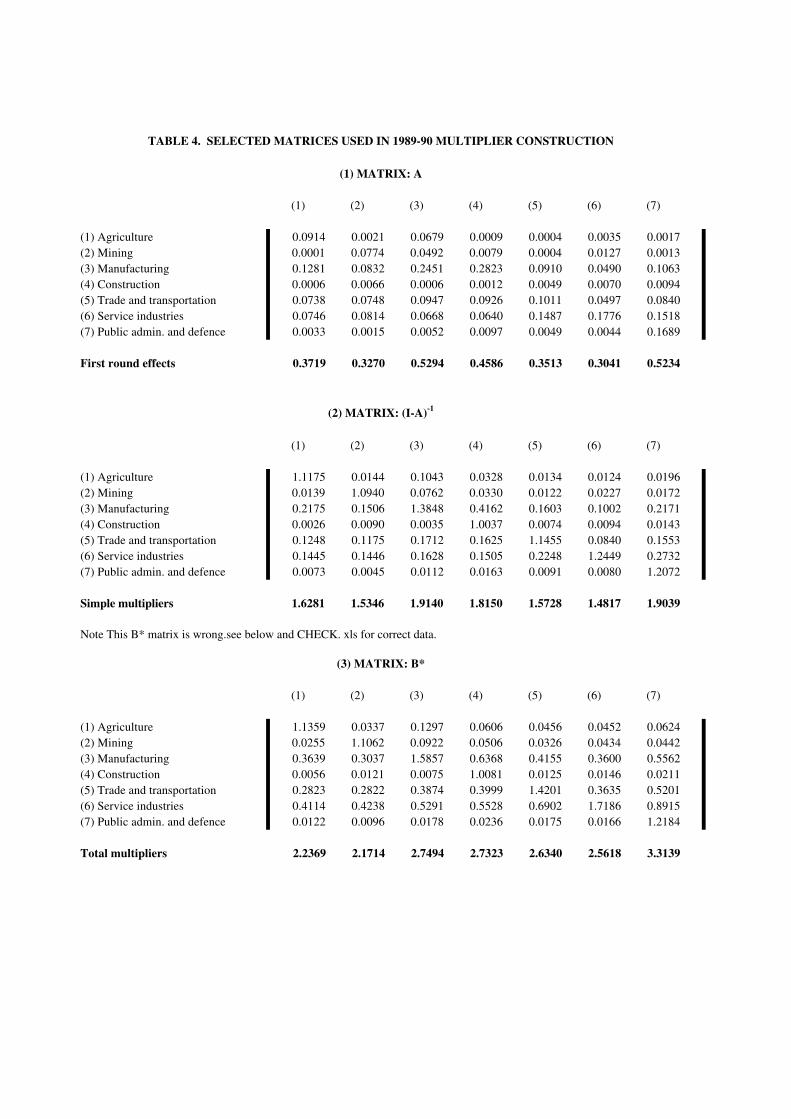
TABLE 4. SELECTED MATRICES USED IN 1989-90 MULTIPLIER CONSTRUCTION

(1) MATRIX: A

(1) (2) (3) (4) (5) (6) (7)

(1) Agriculture 0.0914 0.0021 0.0679 0.0009 0.0004 0.0035 0.0017(2) Mining 0.0001 0.0774 0.0492 0.0079 0.0004 0.0127 0.0013(3) Manufacturing 0.1281 0.0832 0.2451 0.2823 0.0910 0.0490 0.1063(4) Construction 0.0006 0.0066 0.0006 0.0012 0.0049 0.0070 0.0094(5) Trade and transportation 0.0738 0.0748 0.0947 0.0926 0.1011 0.0497 0.0840(6) Service industries 0.0746 0.0814 0.0668 0.0640 0.1487 0.1776 0.1518(7) Public admin. and defence 0.0033 0.0015 0.0052 0.0097 0.0049 0.0044 0.1689

First round effects 0.3719 0.3270 0.5294 0.4586 0.3513 0.3041 0.5234

(2) MATRIX: (I-A)-1

(1) (2) (3) (4) (5) (6) (7)


Simple multipliers 1.6281 1.5346 1.9140 1.8150 1.5728 1.4817 1.9039

Note This B* matrix is wrong.see below and CHECK. xls for correct data.

(3) MATRIX: B*

(1) (2) (3) (4) (5) (6) (7)


Total multipliers 2.2369 2.1714 2.7494 2.7323 2.6340 2.5618 3.3139

12

TABLE 5. MULTIPLIERS

OUTPUT MULTIPLIERS, DIRECT ALLOCATION OF COMPETING IMPORTS, 1989-90

First Industrial Production ConsumptionInitial round support induced induced Simple Totaleffects effects effects effects effects multipliers multipliers


INCOME MULTIPLIERS, DIRECT ALLOCATION OF COMPETING IMPORTS, 1989-90



EMPLOYMENT (FULL-TIME EQUIVALENT) MULTIPLIERS, DIRECT ALLOCATION OF COMPETING IMPORTS, 1989-90


(1) Agriculture 15 4 3 7 7 22 28(2) Mining 4 3 2 5 7 9 16(3) Manufacturing 7 5 4 9 10 16 26(4) Construction 10 4 4 8 10 18 28(5) Trade and transportation 15 4 2 6 12 21 33(6) Service industries 12 3 2 5 12 17 30(7) Public admin. and defence 12 6 4 10 16 22 38

13

GLOSSARY OF TERMS

Terms Simple definition Practical definition

Intermediate inputs (or usage) Commodities that are used in the process ofproduction.

Consists of non-durable goods and services used up in the process of production. Non-durable goods are those having an expected life time use of less than one year.

Primary inputs The inputs into production other than goodsand services.

Inputs into the production process that are notgoods and services. Primary inputs include items such as wages, salaries and supplements (or return to labour) and gross operating surplus(or return to capital) and the various forms ofindirect taxes.

Wages, salaries and supplements Payments by producers to their employees. Payments made by producers to their employeesfor services rendered. They cover income received in cash and kind as well assupplementary benefits.

Gross operating surplus The excess of gross output over the costsincurred in production.

The excess of gross output of enterprises operatingin Australia over costs incurred in producing thatoutput, but before deducting consumption of fixedcapital, dividends, interest, royalties and land rentpayments and direct taxes payable.

Commodity taxes (net) Indirect taxes on certain commodities lesssubsidies.

Indirect commodity specific taxes that are levied on some commodities. Commodity specific subsidies are treated as negativecommodity taxes. Commodity taxes are shown as being paid by the users of the commodity onwhich the tax is levied.

Indirect taxes nec (net) Other indirect taxes less subsidies. Taxes assessed on producers, on the production,sale, purchase or use of goods and services, lesssubsidies. Commodity specific indirect taxes areshown separately as commodity taxes (net).

Sales by final buyers Records the sales of 'second-hand' capitalassets and consumer goods.

In input-output tables this item is necessary torecord the sales of capital assets for scrap and the use of scrap as a raw material in production. It also is used to record net sales ofused motor vehicles.

Competing imports (cif) Commodities purchased from non-residentswhich can be substituted for a locallyproduced commodity.

Competing imports are those importedcommodities which can be substituted fordomestically produced commodities.

Complementary imports (cif) Imported commodities for which there are nolocally produced substitutes.

Complementary imports are those importedcommodities for which there is no domesticallyproduced substitute (e.g. natural rubber).

Australian production The total of intermediate usage and primaryinputs.

The value of goods and services produced by the Australian economy.

Final demand Demand for goods and services not used up in the production process.

Final demand is the sum of Final consumptionexpenditure-private & government; Gross fixedcapital expenditure-private & government;Increase in stocks and Exports of goods andservices.

14

GLOSSARY OF TERMS

Terms Simple definition Practical definition

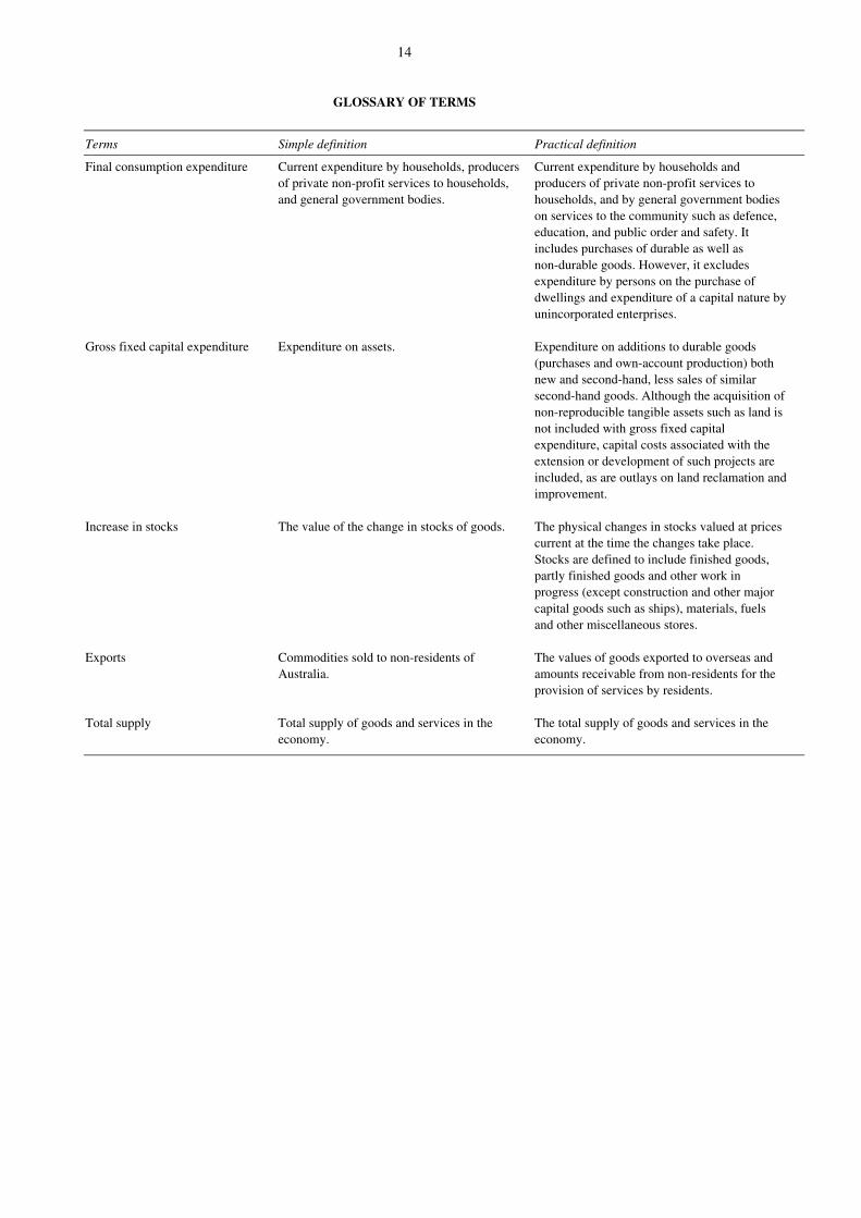
Final consumption expenditure Current expenditure by households, producersof private non-profit services to households,and general government bodies.

Current expenditure by households and producers of private non-profit services tohouseholds, and by general government bodies on services to the community such as defence,education, and public order and safety. It includes purchases of durable as well asnon-durable goods. However, it excludesexpenditure by persons on the purchase ofdwellings and expenditure of a capital nature byunincorporated enterprises.

Gross fixed capital expenditure Expenditure on assets. Expenditure on additions to durable goods(purchases and own-account production) both new and second-hand, less sales of similarsecond-hand goods. Although the acquisition ofnon-reproducible tangible assets such as land isnot included with gross fixed capital expenditure, capital costs associated with theextension or development of such projects areincluded, as are outlays on land reclamation andimprovement.

Increase in stocks The value of the change in stocks of goods. The physical changes in stocks valued at pricescurrent at the time the changes take place. Stocks are defined to include finished goods,partly finished goods and other work in progress (except construction and other majorcapital goods such as ships), materials, fuels and other miscellaneous stores.

Exports Commodities sold to non-residents ofAustralia.

The values of goods exported to overseas andamounts receivable from non-residents for theprovision of services by residents.

Total supply Total supply of goods and services in theeconomy.

The total supply of goods and services in theeconomy.

15

APPENDIX ATECHNICAL NOTE

Assume an economy is divided into n sectors. If we denote by Xi the total output of sector i, Yi the total finaldemand for sector i's product, and Zij the inter-industry sales from sector i to sector j, we may write:

X1 = Z11 + Z12 + ... + Z1j + ... + Z1n + Y1

X2 = Z21 + Z22 + ... + Z2j + ... + Z2n + Y2

.

.

Xi = Zi1 + Zi2 + ... + Zij + ... + Zin + Yi (A.1).

.

Xn = Zn1 + Zn2 + ... + Znj + ... + Znn + Yn

Consider the information in the second row and second column on the right-hand side. The row represents the sales bysector 2, to all the sectors and to final demand; and the column is the sales to sector 2. Thus, the column represents thesources and magnitudes of sector 2's input and the row represents the distribution of sector 2's output. The Z terms onthe right-hand side therefore represent the inter-industry flows of input and output, which can be recorded in a tablecalled an input-output table. These figures (the Z terms) are the core of input-output analysis.

The ratio of input to output, denoted by aij (which equals Zij, the flow of input from i to j, divided by Xj, the totaloutput of j), is termed a technical coefficient. In input-output analysis, a fundamental assumption is that the technicalcoefficients are assumed to be fixed. That is, inputs are employed in fixed proportions. Hence, (A.1) can be rewrittenas:

X1 = a11X1 + a12X2 + ... + a1jXj + ... + a1nXn + Y1

X2 = a21X1 + a22X2 + ... + a2jXj + ... + a2nXn + Y2

.

.

Xi = ai1X1 + ai2X2 + ... + aijXj + ... + ainXn + Yi (A.2).

.

Xn = an1X1 + an2X2 + ... + anjXj + ... + annXn + Yn

In matrix notation, (A.2) is expressed as

X = AX + Y (A.3)

From (A.3) we obtain

X = (I A)-1 * Y (A.4)

If the inverse (I A)-1 exists then (A.4) has a unique solution. The matrix A is known as the direct requirementscoefficients matrix and (I A)-1 is the open Leontief inverse which is frequently referred to as the total requirements

coefficients matrix. In an 'open' input-output model where only the productive sectors of the economy are assumed tobe endogenous (determined by factors inside the productive system), all final demands (private final consumptionexpenditure, government final consumption expenditure, public gross fixed capital expenditure, increase in stocks,

exports) are assumed to be determined by factors outside the productive system. The model, however, can be closed

where: a11 a12 . . a1n X1 Y1 1 0 . . 0

a21 a22 . . a2n X2 Y2 0 1 . . 0

A = . . . , X = . , Y = . and I = . . .

. . . . . . . .

an1 an2 . . ann Xn Yn 0 0 . . 1

16

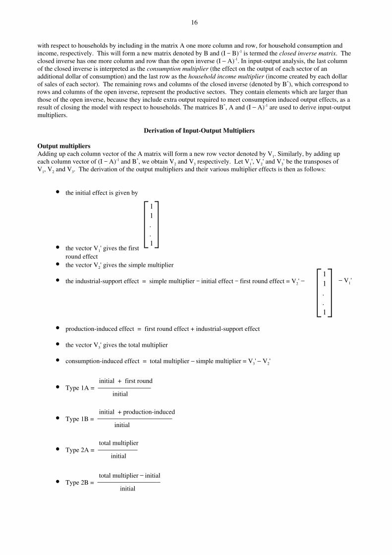
with respect to households by including in the matrix A one more column and row, for household consumption andincome, respectively. This will form a new matrix denoted by B and (I B)-1 is termed the closed inverse matrix. Theclosed inverse has one more column and row than the open inverse (I A)-1. In input-output analysis, the last columnof the closed inverse is interpreted as the consumption multiplier (the effect on the output of each sector of anadditional dollar of consumption) and the last row as the household income multiplier (income created by each dollarof sales of each sector). The remaining rows and columns of the closed inverse (denoted by B*), which correspond torows and columns of the open inverse, represent the productive sectors. They contain elements which are larger thanthose of the open inverse, because they include extra output required to meet consumption induced output effects, as aresult of closing the model with respect to households. The matrices B*, A and (I A)-1 are used to derive input-outputmultipliers.

Derivation of Input-Output Multipliers

Output multipliers Adding up each column vector of the A matrix will form a new row vector denoted by V1. Similarly, by adding upeach column vector of (I A)-1 and B*, we obtain V2 and V3 respectively. Let V1', V2' and V3' be the transposes ofV1, V2 and V3. The derivation of the output multipliers and their various multiplier effects is then as follows:

the initial effect is given by

the vector V1' gives the firstround effect the vector V2' gives the simple multiplier

the industrial-support effect = simple multiplier initial effect first round effect = V2'

V1'

production-induced effect = first round effect + industrial-support effect

the vector V3' gives the total multiplier

consumption-induced effect = total multiplier simple multiplier = V3' V2'

initial + first round Type 1A =

initial

initial + production-induced Type 1B =

initial

total multiplier Type 2A =

initial

total multiplier initial Type 2B =

initial

11..1

11..1

17

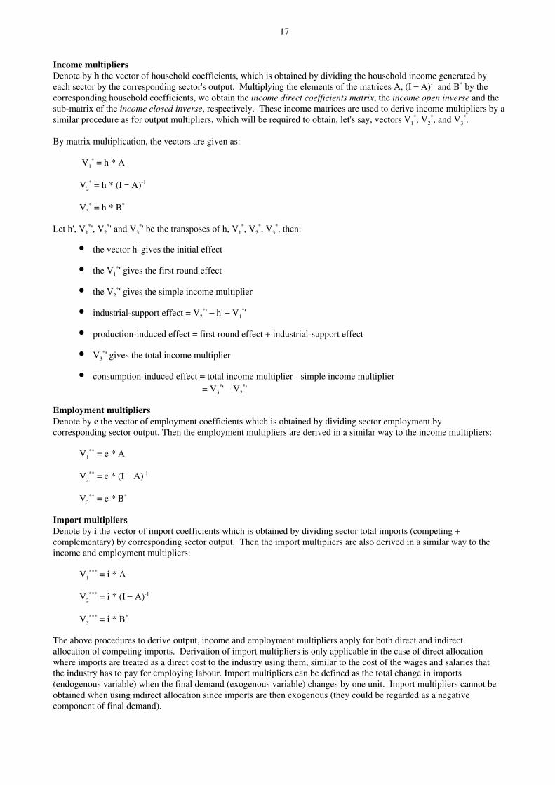
Income multipliers Denote by h the vector of household coefficients, which is obtained by dividing the household income generated byeach sector by the corresponding sector's output. Multiplying the elements of the matrices A, (I A)-1 and B* by thecorresponding household coefficients, we obtain the income direct coefficients matrix, the income open inverse and thesub-matrix of the income closed inverse, respectively. These income matrices are used to derive income multipliers by asimilar procedure as for output multipliers, which will be required to obtain, let's say, vectors V1

*, V2*, and V3

*.

By matrix multiplication, the vectors are given as:

V1* = h * A

V2* = h * (I A)-1

V3* = h * B*

Let h', V1*', V2

*' and V3*' be the transposes of h, V1

*, V2*, V3

*, then:

the vector h' gives the initial effect

the V1*' gives the first round effect

the V2*' gives the simple income multiplier

industrial-support effect = V2*' h' V1

*'

production-induced effect = first round effect + industrial-support effect

V3*' gives the total income multiplier

consumption-induced effect = total income multiplier - simple income multiplier= V3

*' V2*'

Employment multipliers Denote by e the vector of employment coefficients which is obtained by dividing sector employment by corresponding sector output. Then the employment multipliers are derived in a similar way to the income multipliers:

V1** = e * A

V2** = e * (I A)-1

V3** = e * B*

Import multipliers Denote by i the vector of import coefficients which is obtained by dividing sector total imports (competing +complementary) by corresponding sector output. Then the import multipliers are also derived in a similar way to theincome and employment multipliers:

V1*** = i * A

V2*** = i * (I A)-1

V3*** = i * B*

The above procedures to derive output, income and employment multipliers apply for both direct and indirectallocation of competing imports. Derivation of import multipliers is only applicable in the case of direct allocationwhere imports are treated as a direct cost to the industry using them, similar to the cost of the wages and salaries thatthe industry has to pay for employing labour. Import multipliers can be defined as the total change in imports(endogenous variable) when the final demand (exogenous variable) changes by one unit. Import multipliers cannot beobtained when using indirect allocation since imports are then exogenous (they could be regarded as a negativecomponent of final demand).

18

APPENDIX B

ILLUSTRATIVE EXAMPLES

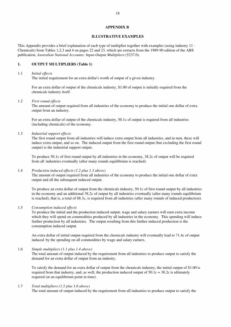
This Appendix provides a brief explanation of each type of multiplier together with examples (using industry 11 -Chemicals) from Tables 1,2,3 and 4 on pages 22 and 23, which are extracts from the 1989-90 edition of the ABSpublication, Australian National Accounts: Input-Output Multipliers (5237.0).

1. OUTPUT MULTIPLIERS (Table 1)

1.1 Initial effectsThe initial requirement for an extra dollar's worth of output of a given industry.

For an extra dollar of output of the chemicals industry, $1.00 of output is initially required from the chemicals industry itself.

1.2 First round effectsThe amount of output required from all industries of the economy to produce the initial one dollar of extraoutput from an industry.

For an extra dollar of output of the chemicals industry, 50.1c of output is required from all industries (including chemicals) of the economy.

1.3 Industrial support effectsThe first round output from all industries will induce extra output from all industries, and in turn, these will induce extra output, and so on. The induced output from the first round output (but excluding the first round output) is the industrial support output.

To produce 50.1c of first round output by all industries in the economy, 38.2c of output will be required from all industries eventually (after many rounds equilibrium is reached).

1.4 Production induced effects (1.2 plus 1.3 above)The amount of output required from all industries of the economy to produce the initial one dollar of extra output and all the subsequent induced output.

To produce an extra dollar of output from the chemicals industry, 50.1c of first round output by all industries in the economy and an additional 38.2c of output by all industries eventually (after many rounds equilibrium is reached), that is, a total of 88.3c, is required from all industries (after many rounds of induced production).

1.5 Consumption induced effectsTo produce the initial and the production induced output, wage and salary earners will earn extra income which they will spend on commodities produced by all industries in the economy. This spending will induce further production by all industries. The output resulting from this further induced production is the consumption induced output.

An extra dollar of initial output required from the chemicals industry will eventually lead to 71.4c of output induced by the spending on all commodities by wage and salary earners.

1.6 Simple multipliers (1.1 plus 1.4 above)The total amount of output induced by the requirement from all industries to produce output to satisfy the demand for an extra dollar of output from an industry.

To satisfy the demand for an extra dollar of output from the chemicals industry, the initial output of $1.00 is required from that industry, and, as well, the production induced output of 50.1c + 38.2c is ultimately required (at an equilibrium point in time).

1.7 Total multipliers (1.5 plus 1.6 above)The total amount of output induced by the requirement from all industries to produce output to satisfy the

19

demand for an extra dollar of output from an industry, and by the spending of the extra wages and salaries earned (from producing the additional output) by householders (consumers).

To satisfy the demand for an extra dollar of chemicals output, the production induced output of $1.883 is required from all industries in the economy, and 71.4c consumption induced output is required from all industries, that is a total of $2.597 output is induced ultimately (at an equilibrium point in time).

1.8 Type 1A (1.1 plus 1.2 above)Type 1B (1.1 plus 1.4 above)Type 2A (1.7 above)Type 2B (1.4 plus 1.5 above)

For output multipliers, these four types are self-explanatory but do not provide information additional to that from the first seven types. For income, employment etc. multipliers, these four types do provide extra information (see below).

2. INCOME MULTIPLIERS (Table 2)

2.1 Each of the seven types of income multipliers (initial, first round, industrial support, production induced, consumption induced, simple and total) corresponds to the additional wages, salaries and supplements earned from working on producing the extra output induced by each of the first seven output effects in 1 above.

Wage and salary earners in the chemicals industry earned an extra 13.4c from working to produce the extra $1.00 of initial output. Wage and salary earners in all industries in the economy earned an extra 11.0c from working to produce the 50.1c of first round output. And so on.

2.2 Type 1AFor a one dollar increase in the wages and salaries earned by income earners in the industry being studied, the amount of additional wages, salaries and supplements earned by income earners in all industries in the economy, after the initial and first round of induced output.

Income earners in the chemicals industry earned an extra one dollar for every $7.463 (i.e. 1/0.134) of additional output. For each one dollar increase in these workers' income, an extra $1.823 is earned byworkers in all industries in the economy, after the initial and first round of induced output.

2.3 Type 1BFor a one dollar increase in the wages and salaries earned by income earners in the industry being studied, the amount of additional wages, salaries and supplements earned by income earners in all industries in the economy, after the initial, first round and industrial support of induced output.

Income earners in the chemicals industry earned an extra one dollar for every $7.463 (i.e. 1/0.134) of additional output. For each one dollar increase in these workers' income, an extra $2.498 is earned by workers in all industries in the economy, after the initial, first round and industrial support induced output.

2.4 Type 2AThe amount of total additional wages and salaries earned by income earners in all industries in the economy due to a one dollar increase in the wages and salaries earned by income earners in the industry being studied. The amount includes the original one dollar increase in wages, salaries and supplements.

Income earners in the chemicals industry earn an extra one dollar for every $7.463 (i.e. 1/0.134) of additional output. For each one dollar increase in these workers' income, an extra $3.836 is earned by workers in all industries in the economy. The amount includes the original one dollar increase in wages and salaries.

2.5 Type 2BType 2B equals Type 2A less the original one dollar increase in wages and salaries.

20

3. GROSS OPERATING SURPLUS (GOS) MULTIPLIERS

These can be interpreted in the same way as the income multipliers except that 'income' refers to wages, salaries and supplements earned by householders; here GOS is earned by businesses.

4. VALUE ADDED AT FACTOR COST MULTIPLIERS

These can be interpreted in the same way as the income multipliers - value added at factor cost being wages, salaries and supplements plus GOS.

5. EMPLOYMENT MULTIPLIERS (Table 3)

5.1 Each of the seven types of employment multipliers (initial, first round, industrial support, production induced, consumption induced, simple and total) corresponds to the additional employment (number of persons employed) generated by producing the extra output induced by each of the first seven output effects in 1 above.

In the tables, the employment multipliers relate to an extra $1 million of output. So for example, for an extra $1 million of output from the chemicals industry, initially an extra 5 persons are employed by that industry. Or one extra worker is employed by the chemicals industry for an extra $200,000 (i.e. 1,000,000/5) of output from that industry.

5.2 Type 1AFor one extra person employed in the industry being studied, the extra number of persons employed in all industries in the economy, after the initial and first round of induced output.

An additional person is employed in the chemicals industry for every $200,000 (i.e. 1,000,000/5) of chemicals output. For each extra person employed in the chemicals industry, an extra 1.968 persons are employed, after the initial and first round induced output.

5.3 Type 1BFor one extra person employed in the industry being studied, the extra number of persons employed in all industries in the economy, after the initial, first round and industrial support induced output.

An additional person is employed in the chemicals industry for every $200,000 (i.e. 1,000,000/5) of chemicals output. For each extra person employed in the chemicals industry an extra 2.761 persons are employed, after the initial, first round and industrial support induced output.

5.4 Type 2AFor one extra person employed in the industry being studied, the total number of extra persons employed in all industries in the economy. The number includes the original increase of one person employed in the industry being studied.

An additional person is employed in the chemicals industry for every $200,000 (i.e. 1,000,000/5) of chemicals output. For each extra person employed in the chemicals industry, an extra 4.441 persons are employed by all industries in the economy. The number includes the original increase of one person employed by the chemicals industry.

5.5 Type 2BType 2B equals Type 2A less the original increase of one person employed by the chemicals industry.

6. COMPETING IMPORTS MULTIPLIERS (Table 4)

6.1 Each of the seven types of competing imports multipliers (initial, first round, industrial support, production induced, consumption induced, simple and total) corresponds to the additional imports required to produce the extra output induced by each of the first seven output effects in 1 above.

21

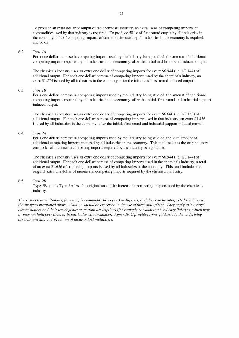
To produce an extra dollar of output of the chemicals industry, an extra 14.4c of competing imports of commodities used by that industry is required. To produce 50.1c of first round output by all industries in the economy, 4.0c of competing imports of commodities used by all industries in the economy is required,and so on.

6.2 Type 1AFor a one dollar increase in competing imports used by the industry being studied, the amount of additional competing imports required by all industries in the economy, after the initial and first round induced output.

The chemicals industry uses an extra one dollar of competing imports for every $6.944 (i.e. 1/0.144) of additional output. For each one dollar increase of competing imports used by the chemicals industry, an extra $1.274 is used by all industries in the economy, after the initial and first round induced output.

6.3 Type 1BFor a one dollar increase in competing imports used by the industry being studied, the amount of additional competing imports required by all industries in the economy, after the initial, first round and industrial support induced output.

The chemicals industry uses an extra one dollar of competing imports for every $6.666 (i.e. 1/0.150) of additional output. For each one dollar increase of competing imports used in that industry, an extra $1.436 is used by all industries in the economy, after the initial, first round and industrial support induced output.

6.4 Type 2AFor a one dollar increase in competing imports used by the industry being studied, the total amount of additional competing imports required by all industries in the economy. This total includes the original extra one dollar of increase in competing imports required by the industry being studied.

The chemicals industry uses an extra one dollar of competing imports for every $6.944 (i.e. 1/0.144) of additional output. For each one dollar increase of competing imports used in the chemicals industry, a total of an extra $1.656 of competing imports is used by all industries in the economy. This total includes the original extra one dollar of increase in competing imports required by the chemicals industry.

6.5 Type 2BType 2B equals Type 2A less the original one dollar increase in competing imports used by the chemicals industry.

There are other multipliers, for example commodity taxes (net) multipliers, and they can be interpreted similarly to the six types mentioned above. Caution should be exercised in the use of these multipliers. They apply to 'average'circumstances and their use depends on certain assumptions (for example constant inter-industry linkages) which mayor may not hold over time, or in particular circumstances. Appendix C provides some guidance in the underlyingassumptions and interpretation of input-output multipliers.

22

TABLE 1. OUTPUT MULTIPLIERS, DIRECT ALLOCATION OF COMPETING IMPORTS, 1989-90

Indust- Prod- Con- First rial uction sumption Simple Total Type 1A Type 1B Type 2A Type 2B

Initial Round Support Induced Induced Multi- Multi- Multi- Multi- Multi- Multi-Indusrty Effects Effects Effects Effects Effects pliers pliers pliers pliers pliers pliers

1 Agriculture 1.000 0.376 0.273 0.649 0.529 1.649 2.178 1.376 1.649 2.178 1.1782 Forestry, fishing, hunting 1.000 0.329 0.255 0.584 0.901 1.584 2.485 1.329 1.584 2.485 1.4853 Mining 1.000 0.327 0.213 0.540 0.596 1.540 2.136 1.327 1.540 2.136 1.1364 Meat and milk products 1.000 0.752 0.544 1.296 0.712 2.296 3.008 1.752 2.296 3.008 2.0085 Food products nec 1.000 0.616 0.491 1.107 0.819 2.107 2.926 1.616 2.107 2.926 1.9266 Beverages, tobacco products 1.000 0.530 0.409 0.939 0.690 1.939 2.629 1.530 1.939 2.629 1.6297 Textiles 1.000 0.553 0.414 0.967 0.811 1.967 2.778 1.553 1.967 2.778 1.7788 Clothing and footwear 1.000 0.446 0.338 0.784 0.965 1.784 2.749 1.446 1.784 2.749 1.7499 Wood, wood products etc 1.000 0.507 0.388 0.895 0.982 1.895 2.877 1.507 1.895 2.877 1.877

10 Paper, printing etc 1.000 0.417 0.277 0.694 0.901 1.694 2.595 1.417 1.694 2.595 1.59511 Chemicals 1.000 0.501 0.382 0.883 0.714 1.883 2.597 1.501 1.883 2.597 1.59712 Petroleum and coal products 1.000 0.604 0.361 0.965 0.473 1.965 2.438 1.604 1.965 2.438 1.43813 Non-metallic min. products 1.000 0.500 0.344 0.844 0.786 1.844 2.630 1.500 1.844 2.630 1.63014 Basic metals and products 1.000 0.570 0.426 0.996 0.646 1.996 2.642 1.570 1.996 2.642 1.64215 Fabricated metal products 1.000 0.548 0.472 1.020 0.891 2.020 2.911 1.548 2.020 2.911 1.91116 Transport equipment 1.000 0.440 0.345 0.785 0.769 1.785 2.554 1.440 1.785 2.554 1.55417 Machinery etc nec 1.000 0.432 0.336 0.768 0.881 1.768 2.649 1.432 1.768 2.649 1.64918 Miscell. manufacturing 1.000 0.458 0.344 0.802 0.839 1.802 2.641 1.458 1.802 2.641 1.64119 Electricity, gas, water 1.000 0.448 0.298 0.746 0.640 1.746 2.386 1.448 1.746 2.386 1.38620 Construction 1.000 0.459 0.354 0.813 0.881 1.813 2.694 1.459 1.813 2.694 1.69421 Wholesale, retail trade 1.000 0.363 0.217 0.580 1.076 1.580 2.656 1.363 1.580 2.656 1.65622 Repairs 1.000 0.290 0.202 0.492 1.057 1.492 2.549 1.290 1.492 2.549 1.54923 Transport, communication 1.000 0.343 0.230 0.573 0.890 1.573 2.463 1.343 1.573 2.463 1.46324 Finance, property etc 1.000 0.323 0.192 0.515 1.096 1.515 2.611 1.323 1.515 2.611 1.61125 Ownership of dwellings 1.000 0.217 0.146 0.363 0.195 1.363 1.558 1.217 1.363 1.558 0.55826 Public admin., defence 1.000 0.523 0.385 0.908 1.325 1.908 3.233 1.523 1.908 3.233 2.23327 Community Services 1.000 0.223 0.144 0.367 1.616 1.367 2.983 1.223 1.367 2.983 1.98328 Recreational etc services 1.000 0.424 0.297 0.721 1.041 1.721 2.762 1.424 1.721 2.762 1.762

TABLE 2. INCOME MULTIPLIERS, DIRECT ALLOCATION OF COMPETING IMPORTS, 1989-90

Indust- Prod- Con- First rial uction sumption Simple Total Type 1A Type 1B Type 2A Type 2B

Initial Round Support Induced Induced Multi- Multi- Multi- Multi- Multi- Multi-Industry Effects Effects Effects Effects Effects pliers pliers pliers pliers pliers pliers


10 Paper, printing etc 0.234 0.115 0.072 0.187 0.225 0.421 0.646 1.490 1.797 2.760 1.76011 Chemicals 0.134 0.110 0.090 0.200 0.178 0.334 0.512 1.823 2.498 3.836 2.83612 Petroleum and coal products 0.026 0.108 0.087 0.195 0.118 0.221 0.339 5.158 8.497 13.049 12.04913 Non-metallic min. products 0.175 0.110 0.082 0.192 0.197 0.367 0.564 1.628 2.097 3.220 2.22014 Basic metals and products 0.115 0.095 0.092 0.187 0.161 0.302 0.463 1.832 2.632 4.042 3.04215 Fabricated metal products 0.204 0.111 0.101 0.212 0.223 0.416 0.639 1.545 2.038 3.130 2.13016 Transport equipment 0.179 0.101 0.079 0.180 0.193 0.359 0.552 1.564 2.009 3.085 2.08517 Machinery etc nec 0.235 0.100 0.076 0.176 0.220 0.411 0.631 1.424 1.750 2.688 1.68818 Miscell. manufacturing 0.205 0.105 0.081 0.186 0.210 0.391 0.601 1.511 1.912 2.936 1.93619 Electricity, gas, water 0.149 0.083 0.067 0.150 0.160 0.299 0.459 1.561 2.010 3.087 2.08720 Construction 0.218 0.110 0.083 0.193 0.221 0.411 0.632 1.502 1.888 2.899 1.89921 Wholesale, retail trade 0.332 0.112 0.058 0.170 0.270 0.502 0.772 1.337 1.513 2.323 1.32322 Repairs 0.372 0.071 0.051 0.122 0.265 0.494 0.759 1.192 1.326 2.037 1.03723 Transport, communication 0.269 0.089 0.058 0.147 0.222 0.416 0.638 1.331 1.542 2.369 1.36924 Finance, property etc 0.360 0.101 0.051 0.152 0.274 0.512 0.786 1.280 1.423 2.186 1.18625 Ownership of dwellings - 0.055 0.036 0.091 0.049 0.091 0.140 - - - -26 Public admin., defence 0.362 0.156 0.101 0.257 0.332 0.619 0.951 1.431 1.712 2.629 1.62927 Community Services 0.652 0.066 0.037 0.103 0.404 0.755 1.159 1.101 1.157 1.778 0.77828 Recreational etc services 0.300 0.114 0.073 0.187 0.260 0.487 0.747 1.382 1.624 2.495 1.495

23

TABLE 3. EMPLOYMENT (FULL-TIME EQUIVALENT) MULTIPLIERS, DIRECT ALLOCATION OF COMPETING IMPORTS,1989-90

Indust- Prod- Con-First rial uction sumption Simple Total Type 1A Type 1B Type 2A Type 2B


1 Agriculture 15 4 3 7 6 22 27 1.266 1.446 1.828 0.8282 Forestry, fishing, hunting 11 3 2 6 10 16 26 1.289 1.516 2.424 1.4243 Mining 4 3 2 5 6 9 15 1.753 2.276 3.977 2.9774 Meat and milk products 5 10 6 16 8 20 28 3.082 4.301 5.922 4.9225 Food products nec 6 7 5 12 9 18 26 2.105 2.955 4.427 3.4276 Beverages, tobacco products 5 6 4 10 7 14 22 2.250 3.124 4.760 3.7607 Textiles 7 6 4 10 9 17 26 1.907 2.550 3.858 2.8588 Clothing and footwear 15 5 4 9 10 24 34 1.353 1.597 2.301 1.3019 Wood, wood products etc 13 6 4 10 11 23 34 1.446 1.738 2.528 1.528

10 Paper, printing etc 9 5 3 7 10 16 26 1.505 1.820 2.903 1.90311 Chemicals 5 4 4 8 8 13 20 1.968 2.761 4.441 3.44112 Petroleum and coal products 1 3 3 7 5 8 13 5.249 9.304 15.595 14.59513 Non-metallic min. products 7 4 3 7 8 14 23 1.609 2.065 3.307 2.30714 Basic metals and products 3 3 3 7 7 10 17 1.922 2.885 4.887 3.88715 Fabricated metal products 9 4 4 8 10 17 27 1.472 1.878 2.922 1.92216 Transport equipment 7 4 3 7 8 14 23 1.570 1.991 3.128 2.12817 Machinery etc nec 10 4 3 7 9 17 26 1.429 1.731 2.720 1.72018 Miscell. manufacturing 10 4 3 8 9 18 27 1.423 1.744 2.614 1.61419 Electricity, gas, water 5 3 2 5 7 10 17 1.567 2.065 3.476 2.47620 Construction 10 5 3 8 9 18 27 1.457 1.781 2.727 1.72721 Wholesale, retail trade 17 4 2 6 12 24 35 1.238 1.367 2.036 1.03622 Repairs 17 3 2 5 11 22 34 1.180 1.293 1.954 0.95423 Transport, communication 11 4 2 6 10 17 26 1.337 1.541 2.429 1.42924 Finance, property etc 12 4 2 6 12 17 29 1.312 1.480 2.491 1.49125 Ownership of dwellings - 2 1 3 2 3 5 - - - -26 Public admin., defence 12 6 4 10 14 21 36 1.475 1.798 2.995 1.99527 Community Services 21 3 1 4 17 25 42 1.122 1.191 2.020 1.02028 Recreational etc services 17 5 3 8 11 24 36 1.290 1.476 2.153 1.153

TABLE 4. COMPETING IMPORT MULTIPLIERS, 1989-90

Indust- Prod- Con-First rial uction sumption Simple Total Type 1A Type 1B Type 2A Type 2B



10 Paper, printing etc 0.131 0.033 0.017 0.050 0.040 0.181 0.221 1.249 1.381 1.686 0.68611 Chemicals 0.144 0.040 0.023 0.063 0.032 0.207 0.239 1.274 1.436 1.656 0.65612 Petroleum and coal products 0.155 0.036 0.022 0.058 0.021 0.213 0.234 1.234 1.374 1.509 0.50913 Non-metallic min. products 0.059 0.027 0.019 0.046 0.035 0.105 0.140 1.454 1.787 2.377 1.37714 Basic metals and products 0.065 0.032 0.024 0.056 0.028 0.121 0.149 1.484 1.852 2.290 1.29015 Fabricated metal products 0.082 0.035 0.028 0.063 0.039 0.145 0.184 1.427 1.758 2.237 1.23716 Transport equipment 0.168 0.037 0.021 0.058 0.034 0.226 0.260 1.220 1.346 1.549 0.54917 Machinery etc nec 0.154 0.033 0.021 0.054 0.039 0.208 0.247 1.216 1.347 1.601 0.60118 Miscell. manufacturing 0.130 0.040 0.021 0.061 0.038 0.191 0.229 1.305 1.475 1.761 0.76119 Electricity, gas, water 0.015 0.016 0.016 0.032 0.028 0.047 0.075 2.066 3.033 4.882 3.88220 Construction 0.061 0.032 0.022 0.054 0.039 0.115 0.154 1.523 1.866 2.502 1.50221 Wholesale, retail trade 0.022 0.018 0.012 0.030 0.048 0.052 0.100 1.830 2.384 4.578 3.57822 Repairs 0.075 0.027 0.013 0.040 0.046 0.115 0.161 1.361 1.531 2.157 1.15723 Transport, communication 0.047 0.024 0.014 0.038 0.040 0.085 0.125 1.502 1.795 2.626 1.62624 Finance, property etc 0.019 0.012 0.010 0.022 0.049 0.041 0.090 1.669 2.200 4.813 3.81325 Ownership of dwellings 0.008 0.008 0.007 0.015 0.009 0.023 0.032 1.930 2.825 3.876 2.87626 Public admin., defence 0.057 0.032 0.023 0.055 0.058 0.112 0.170 1.552 1.945 2.970 1.97027 Community Services 0.028 0.012 0.008 0.020 0.071 0.048 0.119 1.413 1.703 4.257 3.25728 Recreational etc services 0.047 0.019 0.015 0.034 0.046 0.081 0.127 1.399 1.727 2.709 1.709

24

APPENDIX C

UNDERLYING ASSUMPTIONS AND INTERPRETATION OF INPUT-OUTPUT MULTIPLIERS

The basic assumptions in input-output analysis include the following:

there is a fixed input structure in each industry, described by fixed technological coefficients (evidence fromcomparisons between input-output tables for the same country over time have indicated that material inputrequirements tend to be stable and change but slowly; however, requirements for primary factors of production,that is labour and capital, are probably less constant);

all products of an industry are identical or are made in fixed proportions to each other;

each industry exhibits constant returns to scale in production;

unlimited labour and capital are available at fixed prices; that is, any change in the demand for productivefactors will not induce any change in their cost (in reality, constraints such as limited skilled labour orinvestment funds lead to competition for resources among industries, which in turn raises the prices of thesescarce factors of production and of industry output generally in the face of strong demand); and

there are no other constraints, such as the balance of payments or the actions of government, on the response ofeach industry to a stimulus.

2. The multipliers therefore describe average effects, not marginal effects, and thus do not take account ofeconomies of scale, unused capacity or technological change. Generally, average effects are expected to be higherthan the marginal effects.

3. The input-output tables underlying multiplier analysis only take account of one form of interdependence, namelythe sales and purchase links between industries. Other interdependence such as collective competition for factors ofproduction, changes in commodity prices which induce producers and consumers to alter the mix of their purchasesand other constraints which operate on the economy as a whole are not generally taken into account.

4. The combination of the assumptions used and the excluded interdependence means that input-output multipliers arehigher than would realistically be the case. In other words, they tend to overstate the potential impact of final demandstimulus. The overstatement is potentially more serious when large changes in demand and production are considered.

5. The multipliers also do not account for some important pre-existing conditions. This is especially true of Type 2multipliers, in which employment generated and income earned induce further increases in demand. The implicitassumption is that those taken into employment were previously unemployed and were previously consuming nothing.In reality, however, not all 'new' employment would be drawn from the ranks of the unemployed; and to the extent that itwas, those previously unemployed would presumably have consumed out of income support measures and personalsavings. Employment, output and income responses are therefore overstated by the multipliers for these additionalreasons.

6. The most appropriate interpretation of multipliers is that they provide a relative measure (to be compared withother industries) of the interdependence between one industry and the rest of the economy which arises solely frompurchases and sales of industry output based on estimates of transactions occurring over a (recent) historical period.Progressive departure from these conditions would progressively reduce the precision of multipliers as predictivedevices.

25

ANSWERS TO EXERCISE QUESTIONS

INPUT-OUTPUT TABLES

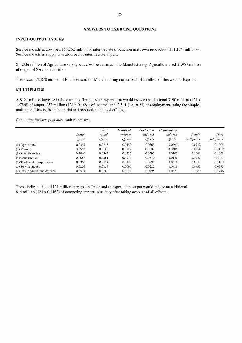
Service industries absorbed $65,252 million of intermediate production in its own production. $81,174 million ofService industries supply was absorbed as intermediate inputs.

$11,336 million of Agriculture supply was absorbed as input into Manufacturing. Agriculture used $1,957 millionof output of Service industries.

There was $78,870 million of Final demand for Manufacturing output. $22,012 million of this went to Exports.

MULTIPLIERS

A $121 million increase in the output of Trade and transportation would induce an additional $190 million (121 x 1.5728) of output, $57 million (121 x 0.4684) of income, and 2,541 (121 x 21) of employment, using the simplemultipliers (that is, from the initial and production induced effects).

Competing imports plus duty multipliers are:

First Industrial Production Consumption Initial round support induced induced Simple Total effects effects effects effects effects multipliers multipliers

(1) Agriculture 0.0347 0.0215 0.0150 0.0365 0.0293 0.0712 0.1005(2) Mining 0.0552 0.0183 0.0119 0.0302 0.0305 0.0854 0.1159(3) Manufacturing 0.1069 0.0365 0.0232 0.0597 0.0402 0.1666 0.2068(4) Construction 0.0658 0.0361 0.0218 0.0579 0.0440 0.1237 0.1677(5) Trade and transportation 0.0356 0.0174 0.0123 0.0297 0.0510 0.0653 0.1163(6) Service indust. 0.0233 0.0127 0.0095 0.0222 0.0518 0.0455 0.0973(7) Public admin. and defence 0.0574 0.0283 0.0212 0.0495 0.0677 0.1069 0.1746

These indicate that a $121 million increase in Trade and transportation output would induce an additional $14 million (121 x 0.1163) of competing imports plus duty after taking account of all effects.

Documents

Information Paper Australian National Accounts ... · interpretation of input-output multipliers. Second, it provides details of the way in which the input-output multiplier tables