inforcement Learning for ssification and Control* · inforcement Learning for ssification and Control* Ming Tan School of Computer Science Carnegie Mellon University Pittsburgh, PA

inforcement Learning for ssification and Control*

Ming Tan School of Computer Science Carnegie Mellon University

Pittsburgh, PA 15213 [email protected]

Abstract Standard reinforcement learning methods assume they can identify each state distinctly before making an action decision. In reality, a robot agent only has a limited sensing capability and identifying each state by extensive sensing can be time consuming. This paper describes an approach that learns active perception strategies in reinforcement learning and considers sensing costs explicitly. The approach integrates cost-sensitive learning with reinforcement learning to learn an efficient internal state representation and a decision policy simultaneously in a finite, deterministic environment. It not only maximizes the long-term discounted reward per action but also reduces the average sensing cost per state. The initial experimental results in a simulated robot navigation domain are encouraging.

Introduction Much like a rat learns to find food in a maze, standard reinforcement learning methods [Watkins 19891 improve a decision policy by receiving rewards from an environment, Unlike traditional planning systems searching throu h a space of action sequences [Fikes & Nilsson 1971 , f they maintain a decision policy to select an action at a state directly. Their reactiv- ity and adaptivity make them suitable in a variety of robot learning tasks such as pole balancing, game play- ing, object manipulation, and robot navigation [Barto, Sutton, & A d n erson 1983, Lin 1991, Sutton 1990, Whitehead & Ballard 199Oa].

However, in order to retrieve relevant decisions, reinforcement learning methods usually assume they have either unlimited sensing capability or a world model (e-g., a map) to identify each individual state distinctly. This assumption is often unrealistic for au- tonomous robots. Even if robots do have unlimited sensing capability, sensing the whole world can be too expensive in practice and impossible in certain environments. Alternatively, a world model could

*This research is supported by DARPA under research contract N00014-85-K-0116 and by NASA under research contract NAGW-1175.

774 ROBOT LEARNING

be first acquired through robot exploration [Rivest & Schapire 19871, but such totally separated model acquisition can be slow and can produce an unnec- essarily detailed model for subsequent reinforcement learning. Recent work [Whitehead & Ballard 1990a, Chapman & Kaelbling 19901 has begun to focus on the importance of learning active perception strategies in reinforcement learning, but they all put certain limits on robot sensory capability (e.g., restricting the number of sensors or the types of sensing features) and ignore the costs of applying sensors (e.g., the speed of a sensor and the time of processing sensory data). As a result, the perception strategies in these systems are neither completely adaptive nor cost-sensitive.

Cost-sensitive learning methods [Tan & Schlimmer 1990b] learn classification knowledge from examples and also construct examples from scratch given class labels. Like reinforcement learning methods, they in- teract with an environment and learn by trial-and- error. Unlike reinforcement learning methods, their learning considers the costs of applying sensors explicitly and is not related to states. They have been ap- plied in classification domains such as object grasping and medical diagnosis [Tan 1990a, Tan 19911.

This paper describes a novel approach that integrates cost-sensitive learning with reinforcement learning in a finite, deterministic environment. In this approach, a cost-sensitive learning method actively senses an environment and learns a task-dependent internal representation that can classify states at low sensing cost. A reinforcement learning method uses the representation to learn a decision policy. In return, it indicates the inadequacy of the internal representation. The two methods bootstrap each other and learn simultaneously and incrementally. The integrated approach has been tested in a simulated robot navigation domain. The experimental results are encouraging.

einforcement Learning

Reinforcement learning is a technique to approximate the conventional optimal control technique known as dynamic programming [Bellman 19571. The external world is modeled as a discrete time, finite state,

From: AAAI-91 Proceedings. Copyright ©1991, AAAI (www.aaai.org). All rights reserved.

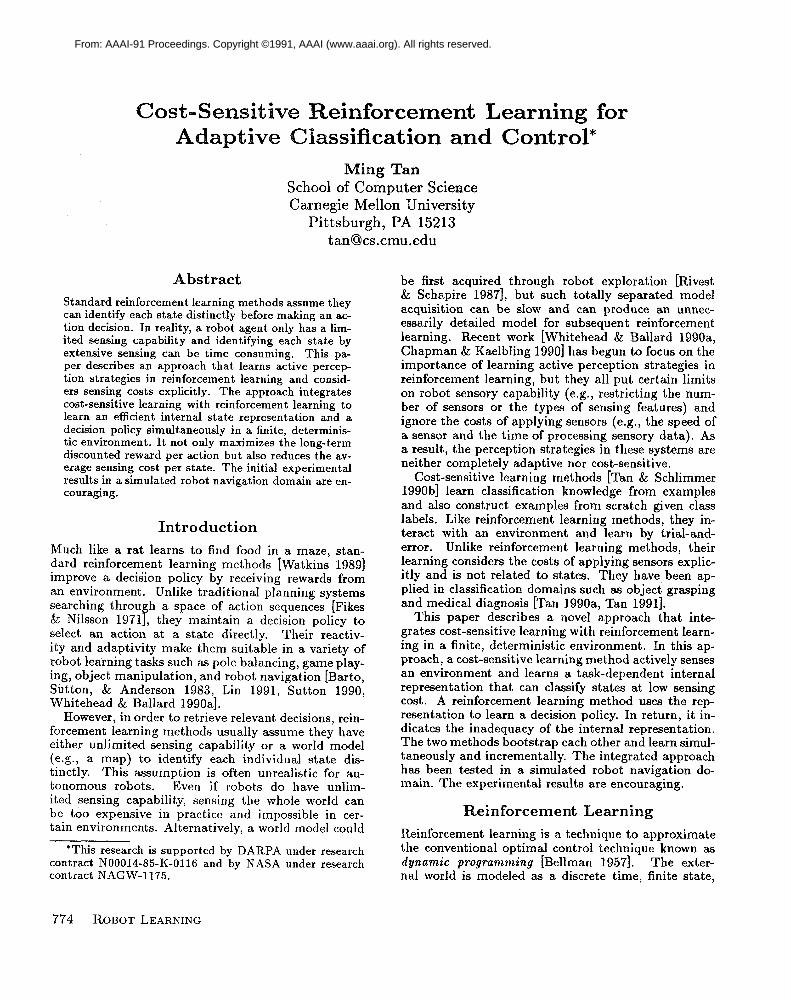
1. z +- the current state. 2. Select an action a according to the Boltzmann distri-

bution: p(ai]z) = eQ(“*ai)/T where 2’ is the

temperature parameter that adjusts the randomness of a decision.

3. Execute action a, and the reward received.

let y be the next state and T be

4. Update the state/action function: Q(E, a) - Q(q a) + P(r + YV(Y) - Qh a)).

5. Update the utility function: V(z) + maxbEactiona Q(z, b).

6. Go to 1.

Figure 1: The Q-learning algorithm.

Markov decision process. Each action is associated with a reward. The task of reinforcement learning is to maximize the long-term discounted reward per action.

One-step Q-learning [Watkins 19891 is a representa- tive reinforcement method. Its learned decision policy, the state/action function Q, tracks expected long-term discounted rewards for each state/action pair. At any state x, the maximum & among possible actions gives the state’s utility,

V(x) - aEEz:n, (ax, 4 0) Moving from state x to state y, a Q-learning agent

updates Q(x, a) by recursively discounting future utilities and weighting them by a postive learning rate ,f?:

&(x:, a) - &(x, 4 + P(r + V(Y) - Qk 4) (2) Here the discount parameter is y (0 < 7 < 1) and T is the reward for executing action a.

As the agent explores the state space, its estimates of Q improve gradually, and, eventually, each V(x) ap- proaches: C,“=r yn-lrt+n. Here ~n~+~ is the reward from the action chosen at time t + n - 1.

Figure 1 outlines the Q-learning algorithm in greater detail. Given a current state x and available actions, select an action a (Step 2) according to the Boltzmann distribution. In Step 3, execute the action, receive a reward, and move to the next state. Then use Equation 2 to update &(x, a) (Step 4). Since updating only occurs when taking action a from state x, using the Boltz- mann distribution ensures that each action will be eval- uated periodically. Watkins [1989] has shown that, for a finite Markov decision process, the state/action function Q learned by the Q-learning algorithm converges to an optimal decision policy. Thus, when the learned decision policy stabilizes and the agent always selects the action having the highest Q value, it will maximize the long-term discounted reward per action.

Most Q-learning methods assume they have unlimited sensing capability to identify each individual state.

This assumption makes them impractical in robot domains where sensing is expensive. One solution is to use active perception that only records the relevant state descriptions in the agent’s internal representation about the external world. However, if the recorded descriptions are insufficient, a Q-learning method may oscillate and fail to converge. Whitehead and Ballard call this phenomenon as “perceptual aliasing” [White- head & Ballard 199Oa]. This occurs when a state description corresponds to multiple nonequivalent states or a state is represented by multiple state descriptions. Whitehead and Ballard only address this problem partially by learning the utilities of a limited number of sensors for memoryless tasks. Chapman and Kaelbling [1990] suggest a different approach: a Q-learning agent first tests all sensing features (which could be expensive) and then selects individually relevant sensing features (which could be insufficient) by statistical tests. A sufficient and efficient internal representation should collapse the state space into a (small) set of equivalence classes and represent each class by a consistent state description, A state description is defined as consistent if and only if its utility and best actions are the same as those of the states that it represents.

Cost-Sensitive Learning Cost-sensitive learning ( CS-learning) is an inductive technique that incrementally acquires efficient classification knowledge from examples, predicts the classes of new objects, and constructs new examples given only correct class labels. A CS-learning method relies on a large number of objects to recognize and exploit their regularities. In practice, objects can be encountered in an arbitrary order. The classes of objects can be either provided by an outside a a robot’s own experimentation Tan 19911. In this pa- B

ent or determined by

per, an example is represented as a set of feature-value pairs plus a class label.

The CS-learning problem can be defined as follows: given (1) a set of unknown objects labeled only by their classes and (2) a set of features whose values for each object can be sensed at known costs, incrementally learn a concept description that classifies the objects by mapping features to classes and minimize the expected sensing cost per object.

Figure 2 outlines a framework for CS-learning that has five generic functions: example attending, feature selection, class prediction, example discrimination, and library updating. By instantiating the five functions proper1 ,

9 a variet of CS-learning methods can be de-

signed Tan 1991 . r For instance, CS-ID3 and CS-IBL [Tan & Schlimmer 1990b] are the cost-sensitive ver- sions of ID3 [Q uin an 1 19861 and IBL [Aha & Kibler 19891 respectively.

As an illustration, consider CS-ID3. For each new object, CS-ID3 first ignores the examples (initially none) that have not matched all its measured values, and from those remaining attended examples selects

TAN 775

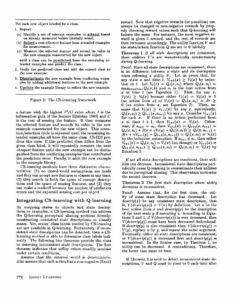
For each new object labeled by a class:

1. Repeat

(4

w (4

Identify a set of relevant examples to attend on already measured values (initially none). Select a cost-effective for measurement.

feature from attended examples

Measure the selected feature and record its value the new example constructed for the new object.

based

in

until a class can be predicted from the remaining attended examples and predict the class.

2. Verify the predicted class and add the correct class to the new example.

3. Discriminate the new example from conflicting examples by adding additional features to the new example.

4. Update the example library to reflect the new example.

Figure 2: The CS-learning framework

a feature with the highest 12/C value where I is the information gain of the feature [Quinlan 19861 and C is the cost of sensing the feature. It then measures the selected feature and records its value in the new example constructed for the new object. This atten- tion/selection cycle is repeated until the remaining attended examples all have the same class. CS-ID3 predicts this class. If this predicted class differs from the given class label, it will repeatedly measure the next cheapest feature until the new example can be distin- guished from the conflicting examples that contributed the prediction error. Finally, it adds the new example to the example library.

CS-learning methods have three distinctive charac- teristics: (1) no closed-world assumptions are made and they can accept new features or classes at any time, (2) they search in both the space of concept descriptions and the space of sensing features, and (3) they can make a tradeoff between the number of prediction errors and the expected sensing cost per object.

Integrating CS-learning with Q-learning

By mapping states to objects and state descriptions to examples, a CS-learning method can address the Q-learning perceptual aliasing problem directly: constructing consistent state descriptions to classify states. Vet, states’ class labels needed by CS-learning are not available in Q-learning. Fortunately, if inconsistent state descriptions can be detected, then a CS- learning method is able to determine class labels indirectly. The following two theorems provide the clues to detecting inconsistent state descriptions. The first theorem indicates that utility values steadily increase under certain conditions.

Assume that the external world is deterministic. Also assume that each action has a non-negative (fixed)

reward. Note that negative rewards (or penalties) can always be changed to non-negative rewards by prop- erly choosing reward values such that Q-learning will behave the same. For instance, the most negative reward is given 0 reward, and the rest of rewards are then increased accordingly. The utility function V and the state/action function & are set to 0 initially. Theorem 1 If all state descriptions are consistent, their utilities V ‘s during Q-learning.

are monotonically nondecreasing

Proof: Since all state descriptions are consistent, there is no difference between a state and its description when referring a utility V. Let us prove that, for any state 2 and time t, Vt+l(x) > Vt(x) by induction on t. Let V,(x) = &t(x, at) where &t(x,at) = maXbEactions Qt(x, b) and al is the best action from 2 at time t (see Equation 1). First, for any 2, Vi(x) > K(x) b ecause either VI(~) = Vo(x) = 0 (no actTon from 2) or VI(~) = Ql(x,ul) = pr 2 0 (an action from t, see Equation 2). Then, assume that Vt (z) 2 Vt - 1 (x) for any x, equivalently, Qt(x, at) 1 &t-1(x, at-i) for any x. Consider Vt+l(x) for each x. If there is no action performed from x at time t + 1, then Vt+l(x) = V,(x). Other- wise, if at+1 = at, then Vt+l(x) = Qt+l(x,ut+l) = Qt(x, at) + P(r + Y%(Y) - Q&w)) >, Qt(x, at-l) + P(r + Y&-I(Y) - Qt-&,a-1)) = Qt(vt) = K(x) by the induction assumption. If at+1 # at, then either &+1(x) = Qt(x,at) = K(z) (no change) or %+1(x) =

Qt+l(wt+l) L Qt+&vt) = Qt(x, at) = K(x) by Equation 1.

If not all state descriptions are consistent, their utilities can decrease. Inconsistent state descriptions periodically cause Q-learning to overestimate their utilities due to perceptual alias&g. the second theorem.

This observation motivates

Theorem 2 The first state description whose utility decreases is inconsistent.

Proof: Assume that, for the first time, the utility of some state description has decreased. Let descrip(x) be any consistent state description, that is, V(descrip(x)) = V(x) by definition. Let a be the best action from x and descrip(y) be the description of the next state y if executing a. According to Equa- tions 2 and 1, if V(descrip(x)) is ever decreased, then V(descrip(y)) must have been decreased beforehand. If descrip(y) is also consistent then V(descrip(y)) = V(y), replace x by y, and repeat the same argument. Eventually, either all state descriptions are consistent, or V(descrip(y)) is decreased first and descrip(y) is inconsistent. In the former case, by Theorem 1, no utility can be decreased. A the latter case must be true.

contradiction. Therefore,

If Theorem 2 is used to detect inconsistent state descriptions, V and Q must be reset to 0 each time after

776 ROBOT LEARNING

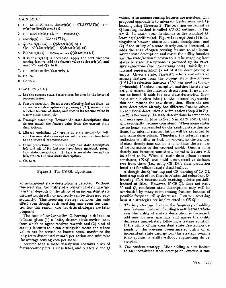
MAIN LOOP:

1. z + an initial state, descrip(z) t CLASSIFY(z), a c- select-action(descrip(z)).

2. y t next-state(x,u), r - reward(y).

3. descrip(y) t CLASSIFY(y). 4. Q(descrip(z), a) t Q(descrip(c), a) +

P(r + yV(descrip(y)) - Q(descrip(z), a)). 5. V(descrip(z)) - =XbEectiona Q(descrip(s), b).

6. If V(descrip(z)) is decreased, apply the next cheapest sensing feature, add the feature value to descrip(z), and reset V’s and Q’s to 0.

7. a t select-action(descrip(y)). 8. 2 - y. 9. Go to 2.

CLASSIFY(state):

1. Let the current representation.

state descriptions be ones in the internal

2. Feature selection: Select a cost-effective feature from the current state descriptions (e.g., using I”/C), measure the selected feature of state, and record its feature value in a new state description.

3. Example attending: Remove the state descriptions that do not match the feature value from the current state descriptions.

4. Library updating: If there is no state description left, add the new state description with a unique class label to the internal representation.

5. Class prediction: If there is only one state description left and ah of its features have been matched, return this state description. If there is no state description left, return the new state description.

6. Go to 2.

Figure 3: The CS-QL algorithm.

an inconsistent state description is detected. Without this resetting, the utility of a consistent state description that depends on the utility of an inconsistent state description directly or indirectly can be decreased sub- sequently. ‘This resetting strategy removes this side effect even though such resetting may seem too dras- tic. For this reason, two heuristic strategies are later proposed.

The task of cost-sensitive Q-learning is defined as follows: given (1) a finite, deterministic environment from which an agent receives rewards and (2) a set of sensing features that can distinguish states and whose values can be sensed at known costs, maximize the long-term discounted reward per action and minimize the average sensing cost per state.

Assume that a state description contains a set of feature-value pairs, a class label, and related V and Q

values. Also assume sensing features are noiseless. The proposed approach is to integrate CS-learning with Q- learning using Theorem 2. The resulting cost-sensitive Q-learning method is called CS-QL outlined in Fig- ure 3. Its MAIN LOOP is similar to the standard Q- learning algorithm (ref. Figure 1) except that (1) it dis- tinguishes between states and state descriptions, and (2) if the utility of a state description is decreased, it adds the next cheapest sensing feature to the inconsistent state description and resets the utility function and the state/action function to 0. The mapping from states to state descriptions is provided by its CLAS- SIFY subroutine (the CS-learning part). Initially, the internal representation (a set of state descriptions) is empty. Given a state, CLASSIFY selects cost-effective sensing features from the current state descriptions (CS-ID3’s selection function 12/C was used in the experiments). If a state description matches the state ex- actly, it returns the matched description. If no match can be found, it adds the new state description (having a unique class label) to the internal representation and returns the new description. Since the new state description already has different feature values, no additional description discrimination (Step 3 in Fig- ure 2) is necessary. As state descriptions become more and more specific (due to Step 6 in MAIN LOOP), they will eventually become consistent. When some states are no longer represented by the existing state descriptions, the internal representation will be expanded by new state descriptions. Therefore, the internal representation is utility or task dependent, so the number of state descriptions can be smaller than the number of actual states in the external world. Once a state description becomes consistent, no extra feature will be added to it. When all state descriptions become consistent, CS-QL can build a cost-sensitive decision tree from them (i.e., using CS-ID3’s class prediction function) for efficient state classification.

Although the Q-learning and CS-learning of CS-QL bootstrap each other, there is substantial redundant Q- learning effort because each resetting deletes partially learned utilities. However, if CS-QL does not reset V and Q, consistent state descriptions may well be overloaded by many extra sensing features because of possible frequent utility decreases. Two non-resetting heuristic strategies are implemented in CS-QL: 1. The lazy strategy: Reduce the frequency of adding

new features. Instead of adding a new feature when- ever the utility of a state description is decreased, add new features sparingly and ignore the utility decreases immediately following a feature addition. If the utility of any consistent state description depends on the previous overestimated utility of an inconsistent state description, this strategy permits it to update its utility without augmenting its description.

2. The random strategy: After adding a new feature to an inconsistent state description, execute a ran-

TAN 777

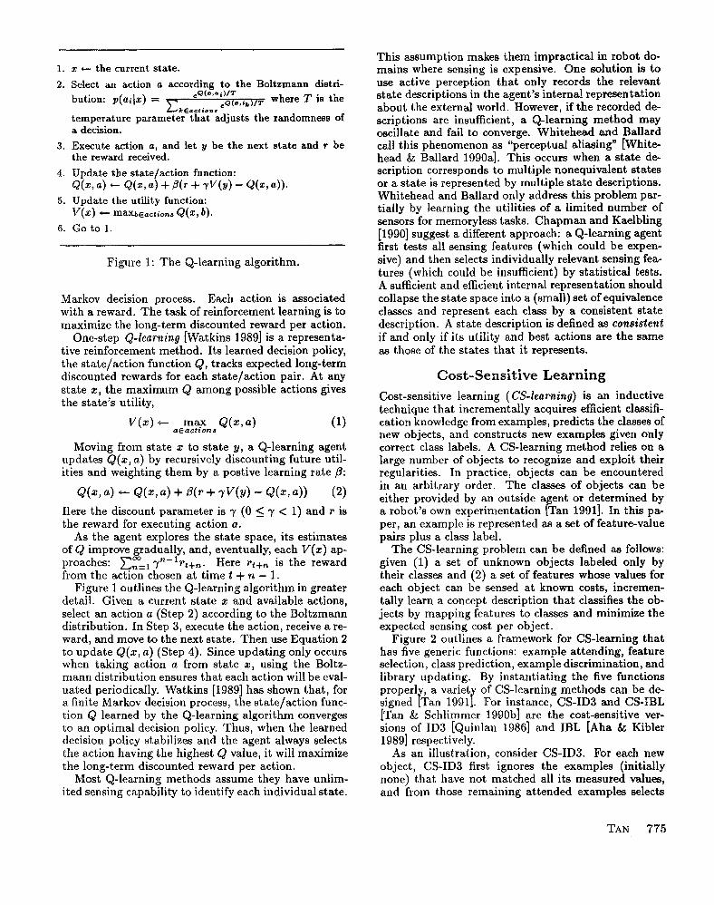
TImdmriptionofthertatewbichir in~qperle&amBsof IimwaM

The dmipticm of the aate which ir nculbalowexlsfLc-oflhswodd,

(a) 04

Figure 4: (a) An 8 by 8 grid world and (b) the examples of state descriptions.

dom sequence of actions that updates the utilities of nearby states, without adding new features to their descriptions. The random strategy differs from the lazy strategy in its active and local utility updating. Random actions also improve state-space exploration. Preliminary experiments indicate that the sensitivity of CS-QL to the number of random actions decreases dramatically as the number of random actions increases.

Both heuristic strategies keep learned utilities intact at the price of possibly adding extra features to consistent state descriptions. This represents a tradeoff between the total sensing cost of learning an internal representation (and policy) and the average sensing cost of classifying a state after learning. The next section will compare the resetting strategy, the lazy strategy, and the random strategy experimentally in these two dimensions.

Experiments in a Navigation

Consider the task of navigating a robot from an arbitrary state to pick up a cup in the 8 by 8 grid world shown in Figure 4[a]. The grid world has 64 states (i.e., cells). The state occupied by a cup is the goal state, the state occupied by the robot is the current state, and the shaded states and the boundary of the grid world are occupied by obstacles and cannot be entered by the robot. On each move, the robot has four possible actions to choose from: walking up, down, left, or right to an adjacent empty state. The reward function is +l for the moves reaching the goal state and 0 otherwise. ’ The robot is able to sense the condition of any neighbor state (i.e., whether it has an obstacle, a cup, or nothing). The conditions of all the neighbor

‘A similar task as h also been studied by Sutton [Sutton 19901 for his Dyna-PI and Dyna-Q reinforcement learning architectures. In contrast to CS-QL, his learning architectures assume that all states can be identified correctly in the beginning.

778 ROBOT LEARNING

lb)

W

Figure 5: A 3 by 3 grid world and the results of learning.

states (including the boundary) constitute the available features of the current state. A neighbor state is referenced by its Cartesian coordinates relative to the robot. The cost of sensing (the condition of) a neighbor state is defined as the sum of the absolute values of its two Cartesian coordinates. Therefore, sensing a distant state is more costly than sensing a nearby one. Initially, the robot agent only has the knowledge of its sensing features and their sensing costs.

As a simple example, given the 3 by 3 grid world shown in Figure S[a], CS-QL learns an internal representation which consists of 7 distinct state descriptions representing 8 states (see Figure 5[b]). CS-QL also learns an optimal decision policy described by the arrows in Figure 5[c]. From the state descriptions, CS- QL can build a cost-sensitive decision tree depicted in Figure 5[d].

In the experiments for the 8 by 8 grid world, each run consisted of a sequence of trials. Each trial started with the robot given a random empty state and ended when the goal state was achieved or a time limit (100 moves) expired. Each run ended when CS-QL con- verged, i.e., every state description was consistent and every state utility was optimal. In other words, the minimal-distance path from any state to the goal state had been found. The Q-learning parameters were set at /3 = 1, 7 = 0.9, and T = 0.4. CS-QL has been tested in other similar tasks by changing the location of a goal state, the size of a grid world, and the layout of a grid world. Similar performance results have been observed.

Table 1 summarizes the experiment results of CS- QL in eight categories (the last four categories were the measurements after convergence): (1) the total sensing cost prior to finding a sufficient internal representation, (2) the total number of trials prior to finding the representation, (3) the total sensing cost prior to convergence, it includes (l), (4) the total number of trials prior to convergence, it includes (2), (5) the number of state descriptions, (6) the average number of features per state description, (7) the maximal number of features in a state description, and (8) the average sensing cost per state, i.e., to classify a state. All

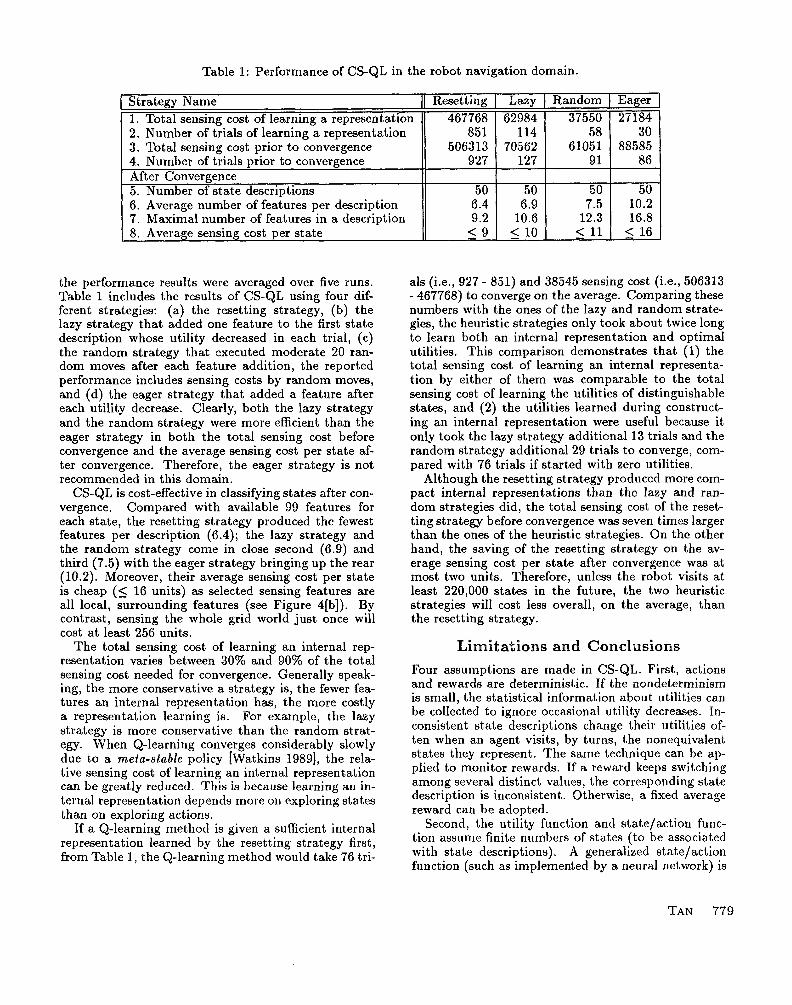
Table 1: Performance of CS-QL in the robot navigation domain.

Strategy Name Resetting Lazy Random Eager 1. Total sensing cost of learning a representation 467768 62984 37550 27184 2. Number of trials of learning a representation 851 114 58 30 3. Total sensing cost prior to convergence 5063 13 70562 61051 88585 4. Number of trials prior to convergence 927 127 91 86 After Convergence 5. Number of state descriptions 50 50 50 50 6. Average number of features per description 6.4 6.9 7.5 10.2 7. Maximal number of features in a description 9.2 10.6 12.3 16.8 8. Average sensing cost per state 19 5 10 5 11 < 16

the performance results were averaged over five runs. Table 1 includes the results of CS-QL using four different strategies: (a) the resetting strategy, (b) the lazy strategy that added one feature to the first state description whose utility decreased in each trial, (c) the random strategy that executed moderate 20 random moves after each feature addition, the reported performance includes sensing costs by random moves, and (d) the eager strategy that added a feature after each utility decrease. Clearly, both the lazy strategy and the random strategy were more efficient than the eager strategy in both the total sensing cost before convergence and the average sensing cost per state after convergence. Therefore, the eager strategy is not recommended in this domain.

CS-QL is cost-effective in classifying states after convergence . Compared with available 99 features for each state, the resetting strategy produced the fewest features per description (6.4); the lazy strategy and the random strategy come in close second (6.9) and third (7.5) with the eager strategy bringing up the rear (10.2). Moreover, their average sensing cost per state is cheap (5 16 units) as selected sensing features are all local, surrounding features (see Figure 4[b]). By contrast, sensing the whole grid world just once will cost at least 256 units.

The total sensing cost of learning an internal representation varies between 30% and 90% of the total sensing cost needed for convergence. Generally speak- ing, the more conservative a strategy is, the fewer features an internal representation has, the more costly a representation learning is. For example, the lazy strategy is more conservative than the random strategy. When Q-learning converges considerably slowly due to a meta-stable policy [Watkins 19891, the relative sensing cost of learning an internal representation can be greatly reduced. This is because learning an internal representation depends more on exploring states than on exploring actions.

If a Q-learning method is given a sufficient internal representation learned by the resetting strategy first, from Table 1, the Q-learning method would take 76 tri-

als (i.e., 927 - 851) and 38545 sensing cost (i.e., 506313 - 467768) to converge on the average. Comparing these numbers with the ones of the lazy and random strategies, the heuristic strategies only took about twice long to learn both an internal representation and optimal utilities. This comparison demonstrates that (1) the total sensing cost of learning an internal representation by either of them was comparable to the total sensing cost of learning the utilities of distinguishable states, and (2) the utilities learned during constructing an internal representation were useful because it only took the lazy strategy additional 13 trials and the random strategy additional 29 trials to converge, compared with 76 trials if started with zero utilities.

Although the resetting strategy produced more com- pact internal representations than the lazy and random strategies did, the total sensing cost of the resetting strategy before convergence was seven times larger than the ones of the heuristic strategies. On the other hand, the saving of the resetting strategy on the average sensing cost per state after convergence was at most two units. Therefore, unless the robot visits at least 220,000 states in the future, the two heuristic strategies will cost less overall, on the average, than the resetting strategy.

imitations and Conclusions

Four assumptions are made in CS-QL. First, actions and rewards are deterministic. If the nondeterminism is small, the statistical information about utilities can be collected to ignore occasional utility decreases. In- consistent state descriptions change their utilities often when an agent visits, by turns, the nonequivalent states they represent. The same technique can be ap- plied to monitor rewards. If a reward keeps switching among several distinct values, the corresponding state description is inconsistent. Otherwise, a fixed average reward can be adopted.

Second, the utility function and state/action function assume finite numbers of states (to be associated with state descriptions). A generalized state/action function (such as implemented by a neural network) is

TAN 779

often needed to classify unknown states, but this will fluctuate state utilities. If an actual utility function is relatively smooth over the state space, thresholds can be used to reduce the sensitivity of CS-QL to the slight changes of utilities, in other words, a state description is considered inconsistent only if its utility is decreased by more than a fixed amount.

Third, sensing is noiseless. Incorrect feature values can cause misclassification. If CS-QL generates each state description such that it is sufficiently different from others, it can use the nearest neighbor match in classifying states to handle bounded sensing noise. Building a cost-sensitive decision tree (as CS-ID3 does) after convergence can also prune some noisy features originally close to leaves.

Fourth, nonequivalent states are distinguishable. If a state cannot be differentiated from others by the features obtainable at the state, CS-QL can use the features obtainable at its neighbor states. This may re- quire additional actions to visit neighbor states. In the extreme case where each state has only one available feature, CS-QL may have to inspect quite a few neighbor states before identifying the current state [Rivest & Schapire 19891.

In summary, this paper describes a novel learning method CS-QL that integrates CS-learning with Q- learning in a finite, deterministic environment. Its Q-learning relies on its CS-learning to classify a state while its CS-learning relies on its Q-learning to indicate whether a state description is inconsistent or not. This paper proves that CS-QL using the resetting strategy learns not only state utilities but also state descriptions. The experiments show that CS-QL using either of the heuristic strategies learns an internal representation and a decision policy efficiently and reduces the average sensing cost per state. From such an internal representation, a task-dependent world model (e.g., a reduced map) can be built through exploring actions at each state. Future work will focus on removing some of its limitations and exploring the possibility of relating sensing costs to rewards.

Acknowledgements

I like to thank Jeff Schlimmer for suggesting the resetting strategy and thank Steven Whitehead, Long-Ji Lin, Rich Sutton, Roy Taylor, and reviewers for pro- viding useful comments on previous drafts.

eferences Aha, D. W., and Kibler, D. 1989. Noise-Tolerant Instance-Based Learning Algorithms. In Proceedings of the Eleventh IJCAI, 794-799. Morgan Kaufmann. Barto: A. G.; Sutton, R. S.; and Anderson, C. W. 1983. Neuron-like Elements That Can Solve Difficult Learning Control Problem. IEEE Trans. on Systems, Man, and Cybernetics, SMC-13(5):834-846.

Bellman, R. E. 1957. Dynamic Programming. Prince- ton University Press, Princeton, NJ. Chapman, D. and Kaelbling, L. P. 1990. Learning from Delayed Reinforcement In a Complex Domain, Technical Report, TR-90-11, Teleos Research, De- cember . Fikes, R. E., and Nilsson, N. J. 1971. Strips: A New Approach to the Application of Theorem Proving to Problem Solving. Artificial Intelligence, 2, 189-208. Lin, L. J. 1991. Programming Robots Using Rein- forcement Learning and Teaching. In Proceedings of the Ninth National Conference on Artificial Intelli- gence, AAAI Press/The MIT Press. Quinlan, J. R. 1986. Induction of Decision Trees. Ma- chine Learning, 1, 81-106. Rivest, R. L., and Schapire, R. E. 1987. A New Ap- proach to Unsupervised Learning in Deterministic Environments. In Proceedings of the fourth Interna- tional Workshop on Machine Learning, 364-375: Mor- gan Kaufmann. Rivest, R. L., and Schapire, R. E. 1989. Inference of Finite Automata Using Homing Sequences. In Pro- ceedings of the Twenty First Annual ACM Sympo- sium on Theory of Computing, 411-420. ACM Press. Sutton, R. S. 1990. Integrated Architecture for Learn- ing, Planning, and Reacting Based on Approximating Dynamic Programming. In Proceedings of the Sev- enth International Conference on Machine Learning, 216-225. Austin, Texas. Tan, M. 1990a. CSL: A Cost-Sensitive Learning Sys- tem for Sensing and Grasping Objects. In Proceed- ings of the 1990 IEEE International Conference on Robotics and Automation, 858-863. IEEE Computer Society Press. Tan, M., and Schlimmer, J. C. 1990b. Two Case Stud- ies in Cost-Sensitive Concept Acquisition. In Proceed- ings of the Eighth National Conference on Artificial Intelligence, 854-860. AAAI Press/The MIT Press. Tan, M. 1991. Cost-Sensitive Robot Learning. Ph.D. thesis, School of Computer Science, Carnegie Mellon University. Watkins, C. J. C. H. 1989. Learning With Delayed Re- wards. Ph.D. thesis, Cambridge University Psychol- ogy Department. Whitehead, S. D., & Ballard, D. H. 1990a. Active perception and reinforcement learning. In Proceedings of the Seventh International Conference on Machine Learning, 179-189. Austin, Texas. Whitehead, S. D., & Ballard, D. H. 1990b. Learning to perceive and act. Manuscript submitted for publi- cation.

780 ROBOT LEARNING

Documents

inforcement Learning for ssification and Control* · inforcement Learning for ssification and Control* Ming Tan School of Computer Science Carnegie Mellon University Pittsburgh, PA