Influence of Upper Tropospheric Disturbances on the

Instructions for use

Title Influence of Upper Tropospheric Disturbances on the Synoptic Variability of Precipitation and Moisture Transport overSummertime East Asia and the Northwestern Pacific

Author(s) Horinouchi, Takeshi

Citation Journal of the Meteorological Society of Japan. Ser. II, 92(6), 519-541https://doi.org/10.2151/jmsj.2014-602

Issue Date 2014-12-25

Doc URL http://hdl.handle.net/2115/59070

Type article

File Information 92_2014-602.pdf

Hokkaido University Collection of Scholarly and Academic Papers : HUSCAP

https://eprints.lib.hokudai.ac.jp/dspace/about.en.jsp

T. HORINOUCHIDecember 2014 519

1. Introduction

The synoptic variability of extratropical weather systems has been studied for many years. Although research has concentrated on the cool (fall to spring)

seasons, some studies cover the summertime. Storm tracks exist over East Asia and the North Pacific (e.g., Blackmon 1976). In the summertime, a track extends from the eastern part of China and the Yellow Sea to the North Pacific over the region of the Japanese islands, and another track extends eastward from the north of the Tibetan Plateau (Whittaker and Horn 1984; Chen et al. 1991; Mesquita et al. 2008). However, their activity is lower than in the cool seasons (Whittaker and Horn 1984; Chen et al. 1991),

Journal of the Meteorological Society of Japan, Vol. 92, No. 6, pp. 519−541, 2014DOI:10.2151/jmsj.2014-602

Influence of Upper Tropospheric Disturbances on the Synoptic Variability ofPrecipitation and Moisture Transport over Summertime East Asia

and the Northwestern Pacific

Takeshi HORINOUCHI

Faculty of Environmental Earth Science, Hokkaido University, Sapporo, Japan

(Manuscript received 25 March 2014, in final form 2 September 2014)

Abstract

This study provides an overall understanding of the summertime synoptic variability of precipitation and moisture transport at mid-latitude from the eastern coastal region of China to the northwestern Pacific. Using satellite precipitation and reanalysis data, a clear relationship is found between upper tropospheric disturbances (Rossby waves), surface precipitation, and lower tropospheric humidity through July and August. The upper tropospheric disturbances are characterized by the undulation of the 1.5 PVU contours of potential vorticity (PV) on the 350 K isentropic surfaces. Case studies suggest that a precipitation band of several hundred kilometers wide and a thousand to several thousand kilometers long is formed very frequently on the equatorward and low-PV side of the northernmost 1.5 PVU contours, which meander together around 40°N. Lower tropospheric specific humidity is also enhanced there, and it falls sharply to the north of these contours. The synoptic situations associated with it include, but are not limited to, a common situation in which moist convection is enhanced ahead of upper-level troughs. These results are confirmed by a composite analysis over the 12 summers from 2001.

A novel method of analyzing the forcing of the quasi-geostrophic potential enstrophy, in which boundary contri-butions are incorporated, reveals that upper tropospheric disturbances in the area are propagated predominantly from the west along the Asian jet, and that they exert a significant forcing onto near-surface levels, while the upward forcing from near-surface levels to upper tropospheric disturbances is weak. A Q-vector analysis shows that the upwelling associated with the precipitation bands is forced predominantly by confluence. This process is frontoge-netic, and surface fronts are often formed therein. The upwelling is enhanced by latent heating. The latitudinal extent of humid air masses is affected not only by this circulation but by low-level flows induced by upper-level distur-bances in a cooperative manner.

Keywords synoptic meteorology; precipitation band; piecewise potential vorticity inversion; water vapor transport; potential enstrophy; summer monsoon

Corresponding author: Takeshi Horinouchi, Faculty of Environmental Earth Science, Hokkaido University, N10W5 Sapporo, Hokkaido 060-0810, JapanE-mail: [email protected]©2014, Meteorological Society of Japan

Journal of the Meteorological Society of Japan Vol. 92, No. 6520

and the baroclinicity and poleward heat transport associated with them are significantly weaker (Nakamura 1992; Ren et al. 2010; Yanase et al. 2014). Therefore, the effect of baroclinic synoptic eddies on summertime weather systems, and in particular on precipitation, is not obvious and is poorly characterized.

Summertime precipitation over East Asia and the extratropical northwestern Pacific has been studied extensively in terms of the East Asian summer monsoon. Moisture is provided from the tropics along the western and northern rim of the North Pacific high, and in early summer the Meiyu–Baiu rain-band is formed. Extensive studies of the meso-scale disturbances along the Meiyu–Baiu frontal zone have covered many aspects, from their climatology to their dynamics (Ninomiya and Akiyama 1992; Ninomiya and Shibagaki 2007, and the references therein), which includes their forcing by means of the piece-wise potential vorticity inversion (e.g., Chen et al. 2003; Tochimoto and Kawano 2012). However, much fewer studies have examined the dynamics of the synoptic Meiyu–Baiu variability (e.g., Akiyama 1990; Chang et al. 1998), and there are even fewer synoptic studies of mid-summer precipitation (e.g., Chen et al. 2004).

In the summertime, upper tropospheric Rossby waves propagate along the Asian jet and break at its exit over the Pacific (see Fig. 1b for the summertime climatology of zonal wind and geopotential height at 200 hPa). Postel and Hitchman (1999) showed that tropopause-level extratropical Rossby wave breaking, defined as the meridional overturning of isentropic potential vorticity contours, is most frequent in summer. One of the regions that experience frequent breaking is the western Pacific where the climatolog-ical potential vorticity contours on the 350 K isen-tropic surface are deflected southward (Fig. 1). This is closer to Eurasia than the corresponding region in winter. Therefore, it may be worthwhile to investigate the effect of propagating or breaking upper tropo-spheric Rossby waves on the synoptic variability of moisture transport and precipitation. As shown below, the effect is indeed significant and explains the overall synoptic variability from the eastern coastal region of China to the northwestern Pacific around 40°N.

This study focuses on July and August. These two months are different from each other in the monsoon context, since the Meiyu–Baiu period typically ends in July, while the mid-summer regime typically holds in August. However, the features found in this study are common to both months, so the statistics

are calculated for the two months together. Sepa-rate results for July and August are mentioned in the text where relevant. The results for June are also mentioned briefly. Note that the impact of the upper tropospheric PV disturbances have been studied rather extensively for the tropics and subtropics (e.g., Kiladis and Weickmann 1992; Yoneyama and Parsons 1999; Waugh and Funatsu 2003; Knippertz 2007).

The rest of this paper is organized as follows. Section 2 introduces the data used. Section 3 presents the relationship found between upper tropospheric disturbances, lower tropospheric moisture, and precip-itation as well as vertical wind. It is hypothesized that the relationship is dominated by the upper tropo-spheric disturbances. In Section 4, the hypothesis is tested using a novel method and further analyzed to elucidate its mechanism. In Section 5, results are discussed from a wider perspective. For instance, surface fronts and seasonality are discussed. Finally, the conclusions are presented in Section 6.

Fig. 1. Twelve-year climatology for July–August, 2001–2012; (a) SST (°C), (b) zonal wind (color shading; m s–1) and geopotential height (contours; interval 50 m) at 200 hPa, and (c) potential vorticity (color shading; PVU) at θ = 350 K.


2. Data

Data over the 12 northern summers of 2001–2012 are used in this study. Statistical analyses cover July and August. The length of the period is sufficient for this study. The results of the composite and statis-tical analyses made in Sections 3 and 4 are almost unchanged by halving the period to 2001–2006 or 2007–2012.

The precipitation dataset used is the Version 7, Tropical Rainfall Measuring Mission (TRMM) Multi-satellite Precipitation Analysis (TMPA) 3B42 product (Huffman et al. 2007) that covers 50°S–50°N. The original spatial and temporal resolutions are 0.25° × 0.25° and 3 hours, respectively, but they are coars-ened to 0.5° × 0.5° and 1 day by spatially binning the daily mean product. The 3B42 dataset is produced by merging microwave and infrared precipitation esti-mates from multiple satellites. The satellite precipita-tion estimates may have large errors. However, they are of sufficient quality for use in this study, in which the overall synoptic variability is studied. Note that the microwave estimates generally have larger errors over land than over ocean.

The other meteorological data used in this study are the National Centers for Environmental Predic-tion (NCEP) and the National Center for Atmospheric Research (NCAR) reanalysis data. The product used has a horizontal resolution of 2.5° × 2.5° and is defined at the 17 standard pressure levels (1000, 925, 850, 700, 600, 500, 400, 300, 250, 200, 150, 100, 70, 50, 30, 20, and 10 hPa). Six-hourly and daily average datasets are available. The daily dataset is mostly used in this study; however, the trajectory calculation in Section 4.4 uses the six-hourly data. The choice of dataset (daily or six-hourly) is justified where required in the text. The daily mean data is used unless other-wise stated. The physical quantities used are zonal and meridional winds, temperature, geopotential height, pressure vertical velocity ω, specific humidity, mean sea-level pressure, and surface pressure. Other quantities such as potential vorticity are derived in this study (see Appendix A).

The NCEP–NCAR reanalysis has been used exten-sively for atmospheric studies, but it is based on a relatively old analysis system. The dataset is neverthe-less used in this study because consistent results are obtained even with it, which suggests some robust-ness.

Monthly mean National Oceanic and Atmospheric Administration (NOAA) Optimum Interpolation (OI) Sea Surface Temperature (SST) data are also used to

show the climatological distribution of SST in Fig. 1.

3. Upper tropospheric influence on moisture transport and precipitation

3.1 Case studyTo investigate the upper tropospheric influence on

the synoptic variability associated with precipitation, various meteorological variables are compared with upper tropospheric fluctuations in Ertel’s potential vorticity (EPV). Figure 2 shows daily mean specific humidity at 850 hPa and the EPV contours of 1.5 and 3 PVU (10–6 K kg–1 m2 s–1) on the 350 K isen-tropic surfaces (potential temperature θ = 350 K) for every other day in July and August, 2010. The 850 hPa specific humidity is generally high over East Asia and the adjacent ocean and has significant day-to-day variation. The humidity at mid-latitude tends to be enhanced in narrow regions on the equatorward and low-EPV side of the 1.5 PVU (or sometimes 3 PVU) contours when the meridional EPV gradient is posi-tive. This feature is especially evident where the 1.5 and 3 PVU contours are relatively close to each other; that is, where there is a well-defined boundary between the tropospheric and stratospheric air masses on the 350 K isentropic surface. The humidity is generally decreased to the north of the EPV contours, and the gradient is often steep over the ocean. Figures for other years exhibit the same features (not shown). The jet stream on the 350 K surface (not shown) tends to follow these EPV contours.

The 850 hPa level is expected to lie near or slightly above the top of the boundary layer of the ocean. At 925 hPa (not shown), which is likely to be within the boundary layer, the specific humidity has the same qualitative features as those at 850 hPa. The 925 hPa humidity also peaks on the equatorward side of the 350 K 1.5 PVU contours, and decreases sharply to the north. However, the humidity at 925 hPa is slightly more homogeneous in the subtropics where the upper-level EPV is relatively low. The results at 700 hPa (not shown) are qualitatively similar to those at 850 hPa, but the equatorward-side peaks located to the south of the upper tropospheric EPV contours are more pronounced.

Figure 3 shows daily precipitation together with the 350 K EPV contours. Narrow bands of precipita-tion, with widths of several hundreds of kilometers, frequently form to the east of the coastal region of China along the upper tropospheric 1.5 PVU contours. The peaks tend to be on the equatorward side of the contours, as with the 850 hPa humidity. Precipita-tion is particularly enhanced where the contours are


Fig. 2. Daily mean 850 hPa specific humidity (color shading) and 350 K potential vorticity (red contours for 1.5 PVU and pink contours for 3 PVU) in July (left) and August (right), 2010. The area covered is 90°E–120°E and 15°N–50°N.


Fig. 3. As in Fig. 2 but for precipitation (color shading; mm day–1). Note that the color scaling is logarithmic.


deflected northward from west to east (e.g., running southwest to northeast). This is a synoptically familiar situation where precipitation is enhanced to the east and west of upper-level lows and highs, respectively. However, precipitation is also frequently enhanced where the EPV contours run zonally or are tilted oppositely (northwest to southeast); that is, precipita-tion can be enhanced ahead of upper-level highs.

The vertical wind ω was also examined at 700 hPa. As expected, the vertical wind is upward where mid-latitude precipitation in Fig. 3 is intense (not shown).

3.2 Composite analysisComposite analysis is conducted to statistically

examine the results shown in the previous section. Figure 4 shows a composite of daily specific humidity (925 and 850 hPa), precipitation, and ω (700 hPa) for the analysis period (Julys and Augusts of the 12 years). Here, the data are first shifted (with interpo-lation) meridionally with respect to the northernmost 1.5 PVU contours on the 350 K isentropic surface and then averaged over time as functions of longi-tude and the relative latitude with respect to the 1.5 PVU contours. Prior to the averaging, screening is applied to restrict data to days when the northern-most EPV contours are continuous over 120°E–180°. Specifically, data are used only when | |φ φi i− ≤+1 10° everywhere between 120°E and 180°, where ϕi is the latitude of the northernmost 1.5 PVU contour at the i-th longitudinal grid point (here, the interval of the grid points is 2.5°). This screening reduced the number of days used in the averaging to approxi-mately one third of the entire period for each of July and August. Figure 4 shows the result only between 120°E and 180° for consistency with the screening. Note that the east coast of China is at around 120°E. On average, the EPV contours are situated at around 40°N as shown in Fig. 4f.

Figures 4a and 4b show the composite specific humidity at 925 and 850 hPa, respectively. Features found in Section 3.1 are reproduced with sharp gradi-ents along the 1.5 PVU contour both at 925 and 850 hPa, and a narrow band of enhanced humidity to the south of the contour. The poleward humidity drop is large to the east of 140°E, over the Pacific Ocean.

Composite precipitation is shown in Fig. 4c. Composite mean values are plotted where the number of data used for averaging is greater than 10. Data missing occurs in the north-west corner, because the TMPA precipitation data are only available up to 50°N. This panel shows that, west of 160°E, precip-

itation is enhanced within a narrow region with a width of 500 km, south of the 1.5 PVU contours. The region shows a gradual northward shift in the relative latitude from west to east. The enhancement is illus-trated more clearly in Fig. 4d, in which the composite precipitation is normalized for each longitude by simply dividing by its latitudinal mean within ±20° in terms of the relative latitude.

Figure 4e shows the composite mean ω at 700 hPa. Its distribution is similar to that of precipitation. The composite vertical wind is revisited in Section 4.3 to investigate adiabatic and diabatic contributions. It is shown there that dynamically forced secondary circulations induce the upwelling where precipita-tion is enhanced. The reason why the relative latitude of composite precipitation and upwelling shows a gradual northward shift from west to east is not clear.

Composites for July and August separately show similar results to Fig. 4 (not shown). The composite result for June is also similar (not shown). Therefore, the features mentioned above are common throughout the northern summer season. However, the concen-tration of precipitation is slightly weaker in August. The composite analysis over July and August has also been conducted without the screening so that all days in July and August for the 12 summers are used (not shown). The result is again similar to Fig. 4, although the concentration of precipitation is reduced, with the peak values of normalized precipitation over the ocean reduced from around 3 to 2.4.

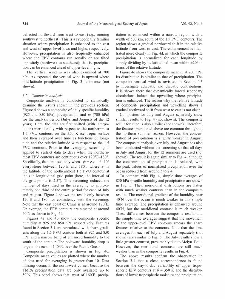
To compare with Fig. 4, simple time averages of 850 hPa specific humidity and precipitation are shown in Fig. 5. Their meridional distributions are flatter with much weaker contrasts than in the composite results. The meridional gradient of the humidity near 40°N over the ocean is much weaker in this simple time average. The precipitation is enhanced around 40°N, but the meridional contrast is much weaker. These differences between the composite results and the simple time averages suggest that the movement of the upper-level EPV contours smears the sharp features relative to the contours. Note that the time averages for each of July and August separately (not shown) are similar to Fig. 5. The July results show a little greater contrast, presumably due to Meiyu–Baiu. However, the meridional contrasts are still much weaker than in the composite results in Fig. 4.

The above results confirm the observation in Section 3.1 that a close correspondence is found between the day-to-day variability of upper tropo-spheric EPV contours at θ = 350 K and the distribu-tions of lower tropospheric moisture and precipitation.


The enhancement of lower tropospheric humidity and upwelling to the south of the 1.5 PVU contours is qualitatively consistent with the enhancement of precipitation.

The EPV contour undulation is supposed to be due to transient Rossby waves (or Rossby wave-like disturbances) that propagate in the upper troposphere eastward along the Asian jet and break over the Pacific. Therefore, the results suggest that the upper tropospheric Rossby waves have a strong influence

on the synoptic variability of the lower tropospheric moisture transport and synoptic precipitation. This hypothesis is tested in the next section.

4. Quasi-geostrophic diagnosis

In the previous section, it was suggested that upper tropospheric potential vorticity disturbances strongly influence the synoptic variability of the moisture transport and precipitation at mid-latitude from the eastern coastal region of China to the northwestern

Fig. 4. Composite means of (a) specific humidity at 925 hPa, (b) specific humidity at 850 hPa, (c) precipitation (mm day–1), (d) precipitation normalized for each longitude, and (e) ω at 700 hPa (contour interval 0.01 Pa s–1). In these panels, the abscissa is longitude and the ordinate is the relative latitude with respect to daily 1.5 PVU contours at 350 K. (f) The mean latitude (°N) of the 1.5 PVU contours used to produce the composites. See text for the composite conditions.


Pacific. However, it may be argued that the vertical association could merely be a consequence of a strong baroclinic vertical coupling, and thus that it might be inappropriate to regard the upper tropospheric distur-bances as the cause. Even though overall baroclinicity is weak in summertime, this possibility should be examined. Vertical forcing (or interaction) processes are investigated in this section, together with the actual mechanism of the synoptic variability of lower tropospheric humidity and precipitation.

The investigation is conducted in the quasi-geos-trophic (QG) framework, under which calculations such as piecewise potential vorticity inversion (PPVI) are conducted. The QG calculations in this study are made under the β-plane approximation with the reference latitude 35°N. The quasigeostrophic poten-tial vorticity (QGPV) is a linear function of the QG stream function. Thus, a merit to use QGPV over EPV to conduct PPVI is its uniqueness due to the linearity. The QG framework also makes theoretical argument easier than with the primitive equations.

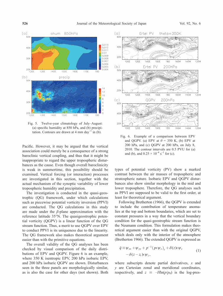
The overall validity of the QG analyses has been checked by visual comparison of the daily distri-butions of EPV and QGPV. Figure 6 is an example, where 350 K isentropic EPV, 200 hPa isobaric EPV, and 200 hPa isobaric QGPV are shown. Disturbances seen in the three panels are morphologically similar, as is also the case for other days (not shown). Both

types of potential vorticity (PV) show a marked contrast between the air masses of tropospheric and stratospheric nature. Isobaric EPV and QGPV distur-bances also show similar morphology in the mid and lower troposphere. Therefore, the QG analyses such as PPVI are supposed to be valid to the first order, at least for theoretical argument.

Following Bretherton (1966), the QGPV is extended to include the contribution of temperature anoma-lies at the top and bottom boundaries, which are set to constant pressures in a way that the vertical boundary condition for the quasi-geostrophic stream function is the Neumann condition. This formulation makes theo-retical argument easier than with the original QGPV, which deals only with the interior of the atmosphere (Bretherton 1966). The extended QGPV is expressed as

�q p p z

z zxx yy z z z

t z

≡ + + ( ) +

− −

−ψ ψ ψ δ ψ

δ ψ

1 ε ε

ε

( )

( ) ,(1)

where subscripts denote partial derivatives, x and y are Cartesian zonal and meridional coordinates, respectively, and z ≡ –Hln(p/p0) is the log-pres-

Fig. 5. Twelve-year climatology of July–August: (a) specific humidity at 850 hPa, and (b) precipi-tation. Contours are drawn at 4 mm day–1 in (b).

Fig. 6. Example of a comparison between EPV and QGPV. (a) EPV at θ = 350 K, (b) EPV at 200 hPa, and (c) QGPV at 200 hPa, on July 8, 2010. The contour intervals are 0.5 PVU for (a) and (b), and 0.25 × 10–4 s–1 for (c).


sure height (H is the constant scale height, set to 7 km in this study, p is pressure, and p0 = 1000 hPa); the bottom and top boundaries are assumed to be at z = 0 and zt, respectively; ψ ≡ (Φ – Φref)/f0 is the quasi-geostrophic stream function (Φ is geopoten-tial, Φref is its reference profile, which is a function only of z, and f0 is the Coriolis parameter at the refer-ence latitude 35°N), while ε≡ f N0

2 2/ is the squared aspect ratio (N is the log-pressure buoyancy frequency derived from the northern mid-latitude summer clima-tology as a function of z), and δ is the Dirac delta function.

If we add infinitesimally thin layers to both vertical boundaries and set ψz = 0 there (i.e., at z = 0 – 0 and z = zt + 0), allowing discontinuities in ψz, Eq. (1) reduces to the same form as the ordinary definition of QGPV:

�q p pxx yy z z= + + ( )−ψ ψ ψ1 ε . (2)

A discretized version of this equation, described in Appendix A, is used for the QGPV in the following. The value of �q at the bottom level, p = 1000 hPa, includes the contribution of the temperature anoma-lies there, irrespective of actual surface pressure (see Appendix A for its validity). The finite difference form of the third term of the rhs of Eq. (2) at 1000 hPa is approximately equal to εψ z d/ there, where d is the thickness of the bottom layer employed in this study (Appendix A). In other words, the contribution of the delta function in (1) is made finite by aver-aging over the finite thickness. It is now evident that one merit of this formulation is that the contribution of the bottom temperature anomalies can be directly compared with that of the interior QGPV. Another merit is its usefulness for potential enstrophy analysis as described below. Its drawback, however, is that PV values depend on the thickness of the bottom layer, which is arbitrarily assumed.

4.1 Mean and perturbation potential vorticity and enstrophy

Figure 7 shows the summer climatology of QGPV, �q, at selected pressure levels. Here and in the following, the overbar denotes the time average taken over the entire July and August periods of the 12 years. The QGPV at 200 hPa (Fig. 7a) exhibits sharp gradients at around 40°N, which roughly corre-sponds to the mean location of the tropopause at that level. The gradient is especially high over the conti-nent owing to the upper tropospheric Asian jet. Also seen at this level, as well as at 300 hPa, is the clima-tological overturning of QGPV over the subtropical

mid Pacific, which is associated with the mid Pacific trough. The gradient is generally weak in the mid troposphere. The poleward gradient of �q is negative at 1000 hPa because of the temperature gradient. Note that the strength of the gradient associated with the bottom temperature gradient is a function of the assumed layer thickness d.

Figure 7 also shows the climatology of the tran-sient part of the potential enstrophy, �′q 2 2/ , where �′q is obtained by subtracting from �q its 15-day running mean. The potential enstrophy at 200 hPa is enhanced where �q has a large gradient. The potential enstrophy at 300 hPa is enhanced at higher latitudes than at 200 hPa, presumably because the tropopause generally intersects with the 300 hPa isobaric surface at higher latitudes. If the running mean period is changed, for example to 7 days or 31 days, the magnitude of the potential enstrophy changes, since the effective spec-tral window is changed. However, its distribution is qualitatively unchanged. In the rest of this paper, the perturbation of a quantity is defined as the deviations from its 15-day running mean, but the results with different running mean periods are mentioned where necessary.

The potential enstrophy at 1000 hPa (Fig. 7h) is enhanced where the meridional gradient of SST (Fig. 1a) is large. This is expected, since �′q there is domi-nated by temperature fluctuation. The perturbation potential enstrophy inside the troposphere is generally smaller than that of the near-surface and tropopausal disturbances (Figs. 7c–g).

4.2 Vertical interactionSince �qy has opposite signs between the upper

troposphere and near the surface, �′q in one of these vertical regions acts to increase the perturbation potential enstrophy in the other, as in the baroclinic instability. However, whether this process is effective in the real atmosphere depends on its amplification rate.

The governing equation for QGPV under the quasi-geostrophic approximation is

∂∂

∂∂

∂∂

∂∂

∂∂

∂∂t u x v y q p x yg g+ +( ) =− + −� ,Q Y Xˆ

(3)

where t is time, ug and vg are the zonal and meridi-onal components of geostrophic winds, respectively, Q is proportional to diabatic heating rate Q as Q ≡ 27

02 2f pQN H

, and X and Y are the frictional acceleration on ug and vg, respectively. Equation (3) can be linear-ized for perturbation as,


( )∂∂

∂∂

∂∂

∂∂

∂∂

∂∂

t u x v y q u q v q

p x y

g g g x g y+ + ′+ ′ + ′

=− ′ + ′ − ′

� � �

.Q Y Xˆ (4)

As mentioned above, the perturbation is defined as the deviation from the 15-day running mean, and the basic state is defined as the climatological time mean. In this case, ′a , where a is an arbitrary phys-ical quantity, is not mathematically zero since ′a is not defined as a – a . However, ′a is neglected from scaling considerations. This means that we neglect the effect of interannual and low-frequency variability on the perturbation.

If we neglect the non-conservative terms on the rhs of Eq. (4), the equation for the quasi-geostrophic potential enstrophy is obtained as follows:

( )∂∂

∂∂

∂∂t u x v y

q

q v q q u q

g g

y g x g

+ + ′

=− ′ ′− ′ ′

ρ

ρ ρ

�

� � � �

2

2

,(5)

where ρ ρ≡ ∝−0e p

zH , and ρ0 is a constant reference

density. If Eq. (5) is time-averaged,

( )u x v y

q

q v q q u q

g g

y g x g

∂∂

∂∂

+ ′

=− ′ ′− ′ ′

ρ

ρ ρ

�

� � � �

2

2

.(6)

Here, the time derivative is neglected because the time averaging is made in the climatological sense. The terms ρ ′ ′v qg � and ρ ′ ′u qg � are the divergences of wave activity fluxes, if the basic state is suffi-ciently slowly varying (Plumb 1986), which is not necessarily the case for the current study. In general, however, remote forcing of the perturbation potential enstrophy is represented by the rhs of Eq. (6), which can be quantified by using the QG PPVI. Appendix C explains the merit of using potential enstrophy over energy in order to quantify vertical interaction. While remote forcing is local and direct in the potential enstrophy budget, it is non-local in the energy budget. A limitation of the potential enstrophy analysis is also stated in Appendix C.

Fig. 7. Twelve-year climatology of July–August mean �q (contours with the interval of 2 × 10–5 s–1) and the tran-sient (periods less than 15 days) potential enstrophy �′q 2 2/ (color shading; s–2) from (a) 200 hPa to (h) 1000 hPa. Regions where the mean surface pressure is lower than 20 hPa minus the pressure of the level (e.g., 980 hPa for the panel h) are masked (treated as missing for graphical purposes only).


The vertical interaction is investigated by using Eq. (6) and QG PPVI. It is done by substituting ′ug and ′vg in Eq. (6) with those obtained by the QG PPVI

from �′q over a limited vertical range. To the author’s knowledge, the type of analysis presented here has not previously appeared in the literature. In what follows, ′ug and ′vg obtained from �′q from p = p1 to p = p2 are

expressed as ′←ug p p[ , ]1 2 and ′←vg p p[ , ]1 2 , respectively (p1 and p2 are written in hPa).

Figure 8a shows − ′ ′←� �q v qy g [ , ]300 200 averaged verti-cally in p over 700–400 hPa.1 If the result is positive (negative), it indicates that the perturbation potential enstrophy forcing is downward (upward) from the upper (300–200 hPa) to the mid (700–400 hPa) tropo-sphere. Positive values are found at around 40°N over the Pacific, indicating downward forcing, while nega-tive values are found at around 50°N especially over the continent, indicating upward forcing. The other forcing term − ′ ′←� �q u qx g [ , ]300 200 (not shown) is weaker and less coherent than − ′ ′←� �q v qy g [ , ]300 200 , as expected.

Figure 8b is similar to Fig. 8a, but the values are divided by �′q 2 2/ averaged over 700–400 hPa. It there-fore shows the potential enstrophy forcing rate, i.e., 1/(e-folding time). Figure 8b shows that the time scale of the forcing mentioned above is on the order of 10 days to the west of the dateline. This is longer than the time scale of horizontal propagation, as will be shown below.

The potential enstrophy forcing of the upper tropo-spheric (200–300 hPa) disturbances from lower levels is also calculated (Fig. 9e). Positive forcing is found in mid-latitude, but it is weak. The e-folding times are typically 20 days over northern Japan and the western Pacific (Fig. 9f). This is much longer than the typical time scale of zonal propagation, which is explained as follows. The zonal propagation of the wave activity is dominated by the advection due to the mean flow, which was confirmed by calculating the wave activity flux of Plumb (1986) (not shown). Mean zonal wind speed in the upper tropospheric mid-latitude jet is around 20 m s–1. The time it takes to travel 4000 km (� 60° zonally at 40°N) at 20 m s–1 is 2 days. There-fore, the perturbation potential enstrophy transport around the jet is dominated by horizontal transport, even though there is some vertical interaction.

The analysis shown above was repeated by using the deviations from the 7-day running mean. The forcing strength is somewhat reduced, as expected, but the forcing time rate is similar to that in Fig. 8b. This is also the case for the interaction with the near-surface level shown below. Using the six-hourly data instead of the daily data in the forcing calculation for Fig. 8 gives very similar results. The validity of using the daily data has also been confirmed for the analyses below except for the trajectory calculations in Section 4.4.

Figure 9 shows the potential enstrophy forcing from the upper and mid troposphere to 1000 hPa, where �′q includes the contribution of the near-surface temperature anomalies. Significant positive forcing

Fig. 8. (a) Potential enstrophy forcing − ′ ′←� �q v qy g [ , ]300 200 averaged between 700 and 400 hPa, which represents the perturbation potential enstrophy forcing from the upper to mid troposphere when positive (color shading with zero-line contours; s–3). (b) Same as (a) but the values are divided by �′q 2 2/ averaged between 700 and 400 hPa so as to represent the temporal e-folding rate (s–1).

1Here, the averaging in p of a quantity f is defined in the form of fdp p pb a

pa

pb/( )−∫ , which corresponds to the averaging in

z after weighting with ρ.


is found around 40°N over the Pacific, where the SST gradient is high (Fig. 1a) and thus �q has a large negative meridional gradient (Fig. 7h). The e-folding time of the forcing is roughly 2 days from the upper troposphere (Fig. 9b) and 1 day from the mid tropo-sphere (Fig. 9d). Therefore, the near-surface potential enstrophy is strongly forced from above.

What this result directly means is that, where low-level winds induced by �′q aloft are southerly (northerly), near-surface �′q is likely positive (nega-tive), so it is amplified, given the sign of �qy. It does not directly tell the origin of the near-surface �′q to be amplified. However, since the current analysis is based on covariances, the contribution of near-sur-face �′q uncorrelated with upper-level �′q should be canceled out statistically. Therefore, given the sign of �qy, the portion of near-surface �′q contributing to the result is explained as induced by upper-level �′q . Therefore, it indicates that the induction and amplifi-cation of near-surface �′q from above is effective.

Since the sign of �qy at 1000 hPa over the mid-lat-itude Pacific, which is negative, is opposite to that above it, the perturbation potential enstrophy forcing from 1000 hPa to the mid and upper troposphere is also positive from Eq. (C5). That is, the near-surface

and mid-to-upper tropospheric disturbances are mutu-ally amplifying as in baroclinic instability. However, the upward forcing from below is weak not only to the upper troposphere as shown above but also to the mid troposphere. Therefore, the vertical potential enstrophy forcing in the region of interest is predom-inantly one-way from the upper troposphere to near surface.

We have neglected the impact of diabatic heating on the perturbation potential enstrophy. However, diabatic heating affects PV as seen in Eq. (3) for QGPV, so its impact is examined here. PV is reduced above the peak of mass-weighted diabatic heating. Therefore, the enhanced condensation heating to the south of the upper-level 1.5 PVU contours acts to enhance or maintain the low PV aloft, a positive feed-back for the composite feature. However, it should be quantitatively minor. The big contrast in PV between the stratospheric and tropospheric air masses is primarily due to the contrast in the static stability. It is not realistic to suppose such a great stability increase to systematically occur on a large scale in the upper troposphere by condensation heating (note also that the 200–300 hPa levels where potential enstrophy is enhanced are well above the mass-weighted heating

Fig. 9. (a, b) As in Fig. 8 but for the potential enstrophy forcing from 300–200 hPa to 1000 hPa and the e-folding rate, respectively. (c, d) Same as (a, b) but from 700–400 hPa to 1000 hPa. Regions where the mean surface pres-sure is lower than 980 hPa are masked. (e, f) Same as (a, b) but from 1000 hPa to 300–200 hPa.


peak). A rough quantitative estimation from Fig. 4c supports it (not shown). Therefore, the above argu-ment based on the dynamical vertical interaction is supported.

4.3 Upwelling mechanismIt is found in Section 3 that both precipitation and

upward wind are enhanced to the south of the 1.5 PVU contours on the 350 K isentropic surfaces. The mechanism driving the upwelling is investigated in this section.

Figure 10 shows the composite divergence of the Q-vector by Hoskins et al. (1978):

∇ ∇Q u≡−

= − + − +

Rp T

f

g

xy xp xx yp yy xp xy yp

( )·

[ , , ],

H H

0 0ψ ψ ψ ψ ψ ψ ψ ψ(7)

where R is the gas constant, and H∇ is the hori-zontal gradient operator. The composite is made in the same way as in Fig. 4 and is shown for 700 hPa. As expected from the omega equation, the Q-vector is convergent where the composite ω in Fig. 4e is negative (upwelling). The convergence is found throughout the troposphere as shown in Fig. 11a. Therefore, the upwelling is interpreted as the ageo-strophic secondary circulation forced by the geos-trophic flows. The convergence is explained almost entirely by Q2, the meridional component of the Q-vector (not shown). Since the temperature gradient is predominantly meridional, this result indicates that the upwelling is mostly induced by confluence; the Q-vector component parallel to the temperature gradient is associated with confluence or difluence, and the fact that the Q-vector convergence is to the south of its divergence (i.e., the composite Q-vector is southward) implies the dominance of confluence. Note that the thermal–wind relationship implies that the upper-level westerly wind is enhanced where the equatorward temperature gradient is enhanced, as metioned in the case study in Section 3.1.

Q-vector analysis is carried out on individual days (not shown). On mid tropospheric pressure levels, the Q-vector below the 350 K 1.5 PVU contour is in many cases enhanced and broadly directed toward the direction of increasing temperature. The results suggest that confluence is the most important factor in inducing upwelling. However, there are cases in which the Q-vector is directed to different directions. Further study would be needed to explain individual cases.

The region where the Q-vector is convergent is tilted in the vertical cross section (Fig. 11a). The region with a relatively strong meridional tempera-

ture gradient is also tilted. Given this morphology and the importance of confluence, the induction of the secondary circulation is by frontogenesis. This is discussed further in Section 5.

The direct influence of upper-level disturbances is investigated using the QG PPVI, but first, the results with and without PV inversion are compared. Figure 11b is the same as Fig. 11a, except that the Q-vector is obtained using the PPVI. Here, Eq. (7) is evalu-ated by substituting ψ with ′ +←ψ ψg [ , ]1000 200 , where ′←ψ g [ , ]1000 200 is obtained from �′q over 1000–200

hPa. The climatological mean term ψ is added in order to retain the contribution of the climatolog-ical temperature gradient. The divergence shown in Fig. 11b is similar to that in Fig. 11a, indicating the validity of the PPVI, but the magnitude is reduced. This is because ′ψ + ψ ≠ ψ . For example, the effect of the year-to-year variability of the background temperature gradient is not incorporated in Fig. 11b.

Figure 11c is the same as Fig. 11b, except that ′←ψ g [ , ]300 200 , obtained from �′q over 300–200 hPa,

is used. Therefore, it shows the dynamical forcing of the secondary circulation by upper-level distur-bances. The convergence near zero relative latitude in the upper troposphere is similar in the two panels. The result indicates that the upper-level disturbances can directly induce upwelling; note that since the omega equation is elliptical, the impact of its forcing is spread out. However, the Q-vector convergence is weaker in the lower troposphere in Fig. 11c than in Fig. 11b. Also, the convergence in the lower tropo-sphere in Fig. 11b is, unlike in Fig. 11c, tilted and

Fig. 10. As in Fig. 4a–e but for ∇⋅Q at 700 hPa. The contour interval is 0.8 × 10–19 kg–1 m s–1. Dashed contours represent negative values (convergence).


enhanced approximately at –5° in the relative latitude. Therefore, mid- to low-level disturbances in �′q asso-

ciated with upper-level disturbances (because we are now examining the composite with respect to upper-level disturbances) are also important, and they shift the upwelling southward.

In order to isolate the contribution of the climato-logical mean geopotential to the Q-vector composite, the same composite is made by using only ψ (by setting the perturbation ψ to zero). The resultant Q-vector divergence composite (not shown) is still negative (convergent) at around the zero relative latitude, but the magnitude is much weaker (smaller than 1/5 of the convergence in Fig. 11a). The meridi-onal extent of the convergent region is approximately 2000 km throughout the troposphere, which is much broader than in Figs. 11a-c. Therefore, the narrow and strong Q-vector convergence in Fig. 11 is asso-ciated primarily with the perturbation geopotential. Note that the broad convergence associated with the climatological geopotential shown here is expected qualitatively from the climatological study of Sampe and Xie (2010) that showed the climatological warm horizontal advection in the Meiyu–Baiu frontal zone (although the analysis period is different).

The importance of the secondary circulation shown in this section does not imply that the upwelling is predominantly adiabatic. The diabatic effect is actu-ally important. Figure 12 shows the composite adia-batic cooling derived from the composite ω between 1000 and 200 hPa. For ease of comparison with precipitation, the adiabatic cooling is divided by the latent heat of water vapor (at 0 °C). A direct compar-ison with Fig. 4c requires the radiative cooling rate to be subtracted from the composite precipitation. A rough estimate suggests that it is about 4 mm day–1. If 4 mm day–1 is subtracted from Fig. 4c and the result compared with Fig. 12, values in these two figures are roughly comparable. It suggests that the latent heating has a significant, leading-order impact on the magnitude of upwelling. There are regions where the diabatic heating rate is even greater than the adiabatic cooling rate, which is inconsistent with the composite convergence of the Q-vector suggesting dynam-ical induction. However, this quantitative compar-ison should not be taken at face value, since the data sources for the two figures are different. Since the Q-vector convergence is likely a robust feature, the composite upwelling can still be concluded as dynam-ically induced, while the upwelling is enhanced significantly via latent heating by reducing the effec-tive static stability. In other words, latent heating plays a significant but passive role.

One might argue that the Q-vector convergence

Fig. 11. (a) e−−32 zH ∇⋅Q composited in the same way as in Fig. 4 and averaged zonally between 130°E and 160°E (color shading; kg–1 m s–1), and temperature processed in the same way (contours with the interval 8 K). A multiplicative factor e−−32 zH is applied such that the scaling is natural for the log-p coordinate, since for W p≡ −12ω , which follows from the standard log-p trans-formation, the omega equation is written as ∂

∂∂

∂∂

∂2

2

2

2

2

2 214x y z H

+ + −

( )ε W p

N H=− 2

32

2 2 ∇⋅Q + (residual

terms). (b) Same as (a) but for e−−32zH ∇⋅Q

obtained by the QG PV inversion (color shading; see text for details) and ∂

∂z g( )[ , ]′ +←ψ ψ1000 200 (contours). (c) Same as (b) but for the piecewise inversion using �′q from 300 to 200 hPa.


shown above could be a result of diabatic heating, indicating the reversed causality. However, it is unlikely, as explained as follows. The Q-vector is associated with the non-divergent geostrophic wind. Therefore, the upper-level divergence associated with the upwelling induced by latent heating does not have a direct impact on the Q-vector. The divergent wind can induce non-divergent wind, but it would likely be difluence, which causes a northward Q-vector peak (rather than a Q-vector convergence peak) that is inconsistent with the composite result. If the diabatic heating is steady, it can induce meridional wind to maintain the steadiness (Hoskins and Karoly 1981). However, the expected meridional wind is not neces-sarily consistent with the composite result. Also, the current composite is made with respect to the mean-dering upper-tropospheric PV contours, and the diabatic heating is far from steady. Thus, the balance does not apply, and it appears that there is no theory of diabatic induction that explains the composite Q-vector convergence.

4.4 Trajectory analysisAs shown in Section 3, low-level specific humidity

is enhanced on the southern side of the upper-level (350 K) EPV contours corresponding to the tropo-pause (e.g., 1.5 PVU). The moisture is provided from low latitudes by the anticyclonic flows associated with the low-level North Pacific high. Visual inspection of daily analyses indicates that the specific humidity

enhancement generally occurs on the periphery of the anticyclone, whose day-to-day variation is affected by dynamical forcing from above.

A trajectory analysis is used here to investigate more quantitatively the role of low-level flow and the effect of upper-level disturbances therein, in the synoptic variability of moisture. In this analysis, passive tracers are advected by the horizontal winds at 850 hPa. Since no vertical advection is allowed, the validity of the analysis is severely limited, but the results below suggest that it is still useful.

As the initial condition, tracers are placed at each of 21 grid points arranged rectangularly at 7 longitudes (115, 120, …, 145°E) and 3 latitudes (20, 25, 30°N). They are advected over 5 days using the six-hourly NCEP reanalysis data. The advection is calculated with a 15-minute time step using the second-order Heun scheme with the 850 hPa winds interpolated linearly in time and bilinearly in space.

Figure 13 shows the 850 hPa specific humidity as well as the 1.5 and 3 PVU contours on the 350 K isentropic surfaces from August 11 to 14, 2010. Their distributions change day by day. For example, on August 11, the 850 hPa specific humidity is rela-tively high over the entire Japan Sea and the Japanese islands. At the same time, the EPV on the 350 K isen-tropic surface is low (tropospheric) there. On August 13, on the other hand, the 850 hPa specific humidity is low and the 350 K EPV is high (stratospheric) over the northern part of the region.

The four panels a–d correspond to start dates of August 6–9. All start times are 00 UTC and the trajectories are calculated over 5 days. The specific humidity and the EPV contours are shown for the final day in each case. The black curves and dots in this figure show the 5-day trajectories and their final positions, respectively. The final positions are in areas of enhanced 850 hPa specific humidity.

The purple curves and dots in this figure are for trajectories advected with [ [ , ]′ +←ug 700 200 u, ′ +←v vg [ , ] , ]700 200 0ˆ , where u and v represent the mean

zonal and meridional winds, respectively, averaged over the 31 days centered on the final day of the tracer advection. Therefore, these trajectories repre-sent advection by the mean winds perturbed by the mid to upper tropospheric QGPV disturbances. The trajectories differ from those advected by the full winds (black in the figure), but their latitudinal extent is similar in each panel. For example, the trajectories extend to higher latitude at around 140°E on August 11 and 12 than on August 13 and 14.

Since the advection is purely horizontal, the distri-

Fig. 12. As in Fig. 10 but for the adiabatic cooling rate at 700 hPa (positive: cooling; negative (dashed): warming). For comparison with precip-itation, the rate is divided by the latent heat of water vaporization and is shown in the units of mm day–1.


bution of the final positions is sensitive to the period of advection and the initial position. However, the present results, including others not shown in the figure, indicate that the overall synoptic association of the upper-level EPV distributions and low-level specific humidity is partly explained by the low-level winds induced by the mid and upper tropospheric perturbations. The sharp contrast in the specific humidity near the upper-level EPV contours is presumably due to the secondary circulation described in the previous section.

5. Discussion

5.1 Surface frontsIn Section 4.3, it was shown that the dynamical

influence from the upper tropospheric synoptic pertur-bations is frontogenetic. Figure 14 shows the 1.5 and 3 PVU contours on the 350 K isentropic surfaces together with the surface weather maps produced by the Japan Meteorological Agency (JMA). The figure suggests that surface quasi-stationary fronts tend to be situated slightly to the south of the upper tropospheric EPV contours. This relation is found to hold at other

times, and also frequently holds for cold fronts.These results indicate that the enhancement of

precipitation to the south of the upper-level EPV contours can also be viewed as the enhancement of precipitation near surface fronts. This is a more tradi-tional view of weather systems. However, the exis-tence of quasi-stationary fronts merely suggests that there are relatively large near-surface temperature gradients that alone reveal little about the dynamics of their formation, especially when they are not associ-ated with extratropical cyclones. Therefore, it is more dynamically meaningful to relate the precipitation bands to upper tropospheric disturbances. In other words, the formation of surface quasi-stationary fronts may be considered as a part of the synoptic systems initiated in the upper troposphere.

5.2 Association with upper-level jet enhancementKodama (1993) showed that satellite-derived

cloudiness of high-level clouds, which is likely asso-ciated with precipitation, in subtropical convergence zones in summertime, such as the Meiyu–Baiu frontal zone, is enhanced when low-level (850 hPa) poleward

Fig. 13. Results of the trajectory analysis. Black solid curves and dots: 5-day trajectories and the final positions, respectively, initialized at (a) August 6, (b) August 7, (c) August 8, and (d) August 9, 2010, using six-hourly hori-zontal winds at 850 hPa. Purple dotted curves and dots: same but using the geostrophic winds obtained by the QG PPVI using �′q between 700 and 200 hPa added to the monthly mean 850 hPa winds. Background color shading shows the specific humidity at 850 hPa at the end of advection (August 11 for (a) to August 14 for (d)). Red and pink curves show the 1.5 and 3 PVU contours, respectively, on the 350 K isentropic surfaces at the end of advec-tion.


Fig. 14. First and third columns from left indicate the following data: 1.5 and 3 PVU contours as in Fig. 2 but using the six-hourly reanalysis data at 00 UTC on every other day from August 7 to 25. Second and fourth columns from left indicate the following data: surface weather maps produced by the JMA for the same time as the EPV contours on the left of each panel (with permission of the JMA).


wind and upper-level (300 hPa) westerly wind are enhanced. As shown in Sections 3.1 and 4.3, westerly wind tends to be enhanced around the 350 K 1.5 PVU contours. Therefore, the results of the present study are consistent with his finding on the importance of upper-level zonal wind, although there are differ-ences in analysis conditions (he established statistical relationship using 10-day mean data at slightly lower latitudes, between 30° and 35°, than in this study). In other words, his findings can be re-interpreted in terms of upper-tropospheric PV disturbances.

The key feature that he found of the impact of the upper-level westerly flow is that the low-level fronto-genesis is statistically enhanced only when the 10-day mean 300 hPa zonal wind is strong (>15 m s–1 as opposed to <5 m s–1; as shown in Fig. 11 of his study). He speculated that when the upper-level jet is strong, it “extends” downward to cause confluence and thereby to increase the low-level frontogenesis. The results of the Q-vector analysis of the present study indicate that the downward influence is realized by the quasi-geostrophic secondary circulation.

5.3 Cut-off lowsCut-off lows have been studied in terms of upper

tropospheric disturbances. Hu et al. (2010) concluded that some 20 % of summer precipitation over north-east China is associated with cut-off lows. High PV anomalies at upper levels destabilize lower levels (e.g., Hoskins et al. 1985) to promote moist convec-tion (e.g., Porcù et al. 2007). This relation (i.e., precipitation underneath upper tropospheric high-PV anomalies) differs from what has been suggested

in this study. Case studies by Zhao and Sun (2007), however, show examples in which precipitation is enhanced to the east of cut-off lows. Their cases might be consistent with this study.

5.4 Cool seasons and tropical moisture exportIn a recent climatological study, Knippertz et al.

(2013) visualized some cases in which column inte-grated water vapor is enhanced near the 2 PVU contours on the 340 K isentropic surface in the boreal cool seasons. The spatial relationship is similar to that shown in this study for summer-time. In addition, we have conducted some preliminary case studies for cool seasons. The spatial relationship between low-level specific humidity and the upper-level EPV contours was broadly similar, but the relationship appeared a little different for precipitation. Knippertz et al. (2013) studied the climatology of tropical mois-ture export to extratropics. This export sometimes takes the form of an “atmospheric river” or “trop-ical plume” (see the review by Knippertz 2007). The atmospheric rivers are frequently associated with cold fronts in developed extratropical cyclones (e.g., Ralph et al. 2004), in which upper tropospheric and near-sur-face disturbances may be tightly coupled.

6. Summary and conclusions

The synoptic variability of precipitation and the associated moisture transport have been studied at mid-latitude from the eastern coastal region of China to the northwestern Pacific using TMPA 3B42 precip-itation data and the NCEP–NCAR reanalysis data over 2001–2012. Statistical analyses cover the July–

Upper-level Rossby waves (E’ward propaga�on breaking)

Moisture transport

200hPa/350K tropopause Secondary Upwelling

Precipita�on / quasi-sta�onary fronts

Fig. 15. Schematic illustration of the synoptic variability of precipitation and the associated moisture transport at mid-latitude from the eastern coastal region of China to the northwestern Pacific (see Section 6). The upper-level PV contour (thick black curve) is illustrated with vertical lines, together like a curtain, to express that it is elevated.


August period. Although the Meiyu–Baiu period typi-cally ends in July, and August is considered to be in the mid-summer regime, the features found in this study are common to the two months. A brief investi-gation has also been made for June.

By investigating the horizontal distributions of daily mean quantities, a clear relationship has been found between upper tropospheric (or tropopausal) disturbances, surface precipitation, and lower tropo-spheric humidity, as illustrated schematically in Fig. 15. Here, the upper tropospheric disturbances are characterized by the undulation of the EPV contours of 1.5 PVU on the 350 K isentropic surfaces (the 3 PVU contours are also used). The low-level humidity at mid-latitude tends to be enhanced in narrow regions on the equatorward and low-EPV side of the EPV contours when the meridional EPV gradient is posi-tive. Narrow bands of precipitating area, with widths of several hundreds of kilometers and lengths of one to several thousand kilometers are frequently formed there. The associated synoptic situations include, but are not limited to, a familiar one in which moist convection is enhanced ahead of upper-level troughs; the precipitation bands along the EPV contours can also appear when the contours run zonally, and they can even appear ahead of upper-level highs.

These features are reproduced in the composite means generated with respect to the northernmost 1.5 PVU contours at the 350 K isentropic surfaces. The composite-mean low level humidity is enhanced to the south of the contours, and decreases sharply to the north. The composite-mean precipitation is remarkably enhanced in a narrow region to the south of the contours. The latitude relative to the 1.5 PVU contours of the region shifts north gradually from west to east. The composite-mean upwelling shows a similar feature. Since the PV contours undulate and move meridionally on a daily basis, simple time averaging smears these features to give much weaker meridional contrasts.

The causality of this association has been investi-gated in the quasi-geostrophic framework. The QGPV used in this study, �q , is the extended definition in which temperature anomalies at the top and bottom boundaries are included. The vertical interaction of transient disturbances can be quantified by examining the forcing of the mean potential enstrophy �′q 2 2/ by utilizing the QG PPVI in a novel manner. The upper-tropospheric perturbation potential enstrophy in the region of interest is provided predominantly from the west along the Asian jet. While the upward forcing from below to the upper tropospheric disturbances is

quite minor, the downward forcing on the near-surface (1000 hPa) potential enstrophy is significant, with a characteristic e-folding time scales of 2 days for forcing originating from the upper troposphere and 1 day from the mid troposphere. Therefore, the dynam-ical forcing is predominantly downward there.

The composite Q-vector indicates that the upwelling associated with the narrow bands of precip-itating area to the south of the 1.5 PVU contours is dynamically forced, predominantly by confluence. The upper-level PV disturbances can directly induce upwelling, but it is enhanced and shifted southward by the associated mid- to low-level disturbances. Latent heating there plays a significant but passive role to reduce the effective static stability. The trajec-tory analysis conducted in this study indicates that the latitudinal extent of humid air masses from the subtropics is partly explained by the low-level flow variability induced by upper-level disturbances.

Surface quasi-stationary fronts tend to be situated to the south of the 1.5 PVU contours at the 350 K isentropic surfaces. Therefore, the relationship found in this study corresponds to precipitation enhance-ment near surface fronts, which is a more traditional view of weather systems. However, the existence of quasi-stationary fronts merely indicates that there are relatively large near-surface temperature gradients. Therefore, it is not a cause. From the dynamical point of view, it is arguably more meaningful to view the synoptic variability as initiated in the upper tropo-sphere and to place the formation of surface quasi-sta-tionary fronts as an aspect of the variability.

This study provides an overall understanding of the synoptic variability of summertime precipitation and the associated moisture transport from a single point of view, and therefore does not aim to explain all synoptic variability. Further studies are needed for a comprehensive understanding.

Appendix A: Finite differentiationand the finite form of QGPV

The data used in this study are equally spaced with longitude and latitude. Thus, horizontal numerical derivatives are evaluated with the central differenti - ation as ∂

∂Ax

A Axi

i i( ) = −∆

+ −1 1

2 and ∂∂Ay

A Ayj

j j( ) = −∆

+ −1 1

2 , where A is an arbitrary quantity and i and j represent grid indices. This scheme has a smoothing effect compared with the differentiation using two adjacent grid points (e.g., ∂

∂Ax

A Axi

i i( ) =−∆+

+12

1) or spectral

differentiation, but it is sufficient for this study. Note


that high wavenumber features are relatively unim- portant for PPVI. To evaluate ∂

∂ ∂

2Ax y , the above two

formula are applied consecutively. Second derivatives are evaluated as ∂

∂

2

2Ax i

=

A AxAi ii+ −− +∆

1 12

2 .

The vertical grid of the reanalysis data is unequal whether with p or z. To secure the second-order accu-racy, vertical derivatives are evaluated as follows: ∂

∂Ap k

k k ks A t s A t Ast s t

=

+ − −+

+ −2

12 2 2

1( )( ) , where s = pk –

pk–1 and t = pk + 1 – pk.To derive the QGPV, the third term of Eq. (2), p−1

( )p z zεψ , is evaluated as follows. For the k-th pressure level, where k = 1, …, K – 1 corresponding to the standard pressure levels 1000 to 70 hPa, it is discret-ized as

1

21 1

1

12

p p

p z z

p

z z k

kk k

k k

∂∂

∂∂ε

ε

ψ

ψ

( )

=

−

+ −−

+ +( ) ( 11

1

12

1

1

−

−−

−

−

+

− −

−

ψ ψ ψk

k k

k k k

k kz z

p

z z

) ( ) ( ),

ε

(A1)

where subscripts denote vertical levels, and values at half-integer levels are defined as 1

2( )p

kε+≡

12 1[( ) ( ) ]p pk kε ε+ + . Levels 1 and K – 1 are dealt

with by introducing two additional levels, 0 and K, at 1075 and 40 hPa, where values are set equal to those at 1000 and 70 hPa, respectively. This is the discrete form to treat the extended QGPV �q . For k = 1, the rhs of Eq. (A1) is approximately equal to d –1 ε

∂∂ψz( )+1 12

, where d ≡ − =z z2 02 1.05 km.

In the NCEP reanalysis, atmospheric quantities are extrapolated down to 1000 hPa even where surface pressure is less than 1000 hPa. This feature is conve-nient for setting the bottom boundary uniformly at 1000 hPa, as done in this study. The value of �q at p much greater than surface pressure has no physical meaning. However, the downward extrapolation does not affect the PV inversion for the atmospheric inte-rior. Therefore, mathematical consistency is not lost. Note that the bottom boundary could alternatively be set at the topographical boundary as in Schneider et al. (2003) for EPV. This approach is not employed in this study.

Appendix B: Quasi-geostrophicpotential vorticity inversion

The QG PPVI in this study uses the Fourier trans-form in the horizontal directions and the Green’s func-tion in the vertical direction. The Fourier transform in the zonal direction is the ordinary complex Fourier transform using the entire longitudinal range. In the meridional direction, the computational domain is taken from 10°N to 65°N, where �′q equatorward of 25°N and poleward of 50°N is tapered by the half-co-sine window. The sine transform is used for the meridional Fourier transform to match the Dirichlet condition at the lateral boundaries.

Since the QGPV in this study is extended to include the contribution of bottom and top temperature anom-alies, the top and bottom boundary condition is the homogeneous Neumann condition such that ′ψ z = 0 at z = 0 – 0 and z = zt + 0. Therefore, it is consis-tent to assume the same Neumann condition for the inversion. In this case, an inconsistency can arise if the volume integral of �′q is not zero when the inver-sion is piecewise (Hakim et al. 1996). This problem, however, is negligible in the present study, since the partitioning is only in the vertical direction.

If ε is constant, the Green’s function to obtain f (k, l) from r (k, l) in Eqs. (C1) and (C2) under the Neumann condition is expressed analytically as follows:

G z z k lg z z k l z zg z z k l z zu

l( , , , )

( , , , )( , , , )

,′ =′ ≥ ′

′ ≤ ′

forfor

(B1)

g z z k l

m e m e m e m em

u

m z zt m z zt mz mz

( , , , )( ) ( )

′ ≡

+ +( )−−

+− −

−′

+− ′ε

2 mm m e emzt mzt− +−−( )

,

(B2)

g z z k l

m e m e m e m em

l

mz mz m z zt m z zt

( , , , )( ) ( )

′ ≡

+( ) + − +−

−′−

+− ′−ε

2 mm m e emzt mzt− +−−( )

,

(B3)where the delta function anomaly is at ′z , k and l are the zonal and meridional wavenumbers, respectively, m k l H≡ +( )+− −ε 1 2 2 2 14( ) , m m H+

−≡ + ( ) ,2 1

and m m H−−≡ − ( )2 1 . When the QG PV inversion

is used in this study, ε is set to a constant by setting N2 = 1.5 × 10–4 s–1. Note that

g z z k l g z z k lu l( , , , ) ( , , , )′ = ′ . (B4)

from Eqs. (B2) and (B3)The inversion conducted in this study is not precise


in the sense that the resultant ψ or ′ψ is not iden-tical to the input one. This is because of the mismatch between the forward and inverse procedures. While the inverse procedure to compute �q (or �′q ) is based on finite difference and vertically varying ε , the backward procedure is based on the Fourier trans-formation, the analytic Green’s functions, and the constant ε . However, the rms error is typically a few % away from the lateral boundaries, and it does not significantly affect the results of this study.

Appendix C: A note on the vertical interactionof potential enstrophy and energy

The vertical interaction of QGPV perturbations are characterized more directly with potential enstrophy than with energy. Following Robinson (1989), this point is demonstrated here in terms of horizontal aver-ages. A remark on the vertical resolution of the anal-ysis is also presented below.

If ′ψ and �′q are written in terms of their Fourier transforms as

′ =

∫∫+ +ψ Re f z t k l e dkdl

zHikx ily( , , , ) ,2 (C1)

�′ =

∫∫+ +q r z t k l e dkdl

zHikx ilyRe ( , , , ) ,2 (C2)

f can be derived from r using the Green’s func-tion, as described in Appendix B. The way in which vertical interaction occurs can be illus-trated mathematically using horizontal averaging, a A a dx dy≡ ∫∫1 , where A is the area of the

domain considered. It follows

ρ ′ ′ ∝ ′ ′∫∫∫v q Z z z k l dz dk dlg � ( , , , ) , (C3)

where

Z z z k l

G z z k l ik r z t k l r z t k l

( , , , )

( , , , ) ( , , , ) *( , , , ) .

′ ≡

′ ′{ }Re(C4)

Here, the asterisk denotes a complex conjugate, and G is the Green’s function defined in Appendix B. From Eq. (B4),

Z z z k l Z z z k l( , , , ) ( , , , ).′ =− ′ (C5)

Therefore, the vertical interaction is symmetric. If the basic state has an appropriate symmetry in a horizontal direction to allow definition of a pseudo- momentum (e.g., ρ �

�′qqy

2

2 if the basic state is zonally

symmetric), there is an action-reaction law in the

vertical forcing of the pseudo-momentum. Robinson (1989) utilized this law to investigate the Charney problem of baroclinic instability.

On the other hand, the vertical interaction is non-local in terms of energy. This is because an addi-tional vertical integration is needed in the energy equation (see Robinson 1989, for formulation using Z).

Even when the basic state is not symmetric, the symmetry represented by Eq. (C5) makes the poten-tial enstrophy suitable for investigating vertical inter-action. This is the reason why potential enstrophy is used in this study.

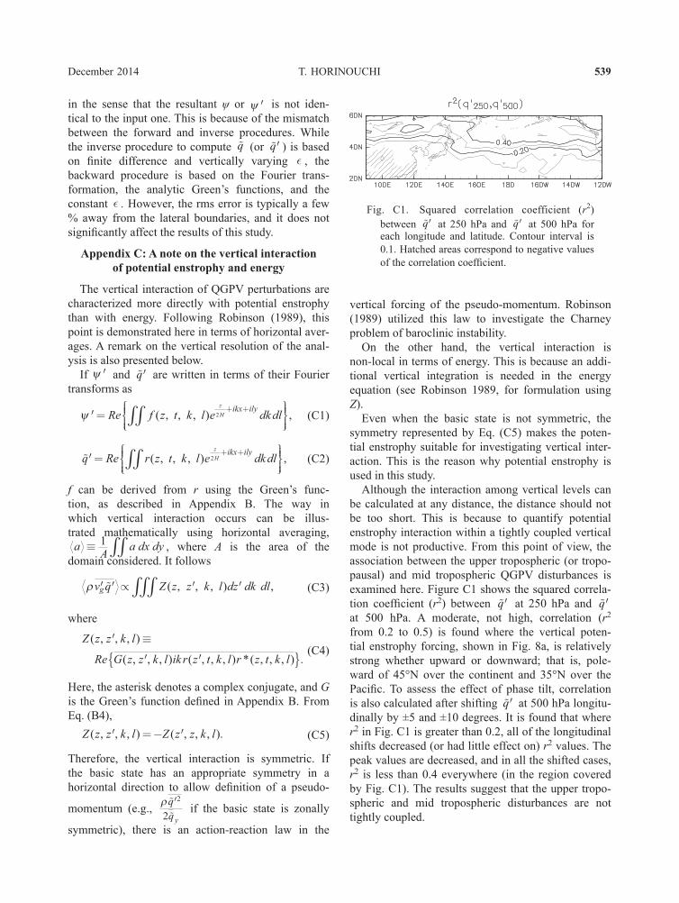
Although the interaction among vertical levels can be calculated at any distance, the distance should not be too short. This is because to quantify potential enstrophy interaction within a tightly coupled vertical mode is not productive. From this point of view, the association between the upper tropospheric (or tropo-pausal) and mid tropospheric QGPV disturbances is examined here. Figure C1 shows the squared correla-tion coefficient (r2) between �′q at 250 hPa and �′q at 500 hPa. A moderate, not high, correlation (r2 from 0.2 to 0.5) is found where the vertical poten-tial enstrophy forcing, shown in Fig. 8a, is relatively strong whether upward or downward; that is, pole-ward of 45°N over the continent and 35°N over the Pacific. To assess the effect of phase tilt, correlation is also calculated after shifting �′q at 500 hPa longitu-dinally by ±5 and ±10 degrees. It is found that where r2 in Fig. C1 is greater than 0.2, all of the longitudinal shifts decreased (or had little effect on) r2 values. The peak values are decreased, and in all the shifted cases, r2 is less than 0.4 everywhere (in the region covered by Fig. C1). The results suggest that the upper tropo-spheric and mid tropospheric disturbances are not tightly coupled.

Fig. C1. Squared correlation coefficient (r2) between �′q at 250 hPa and �′q at 500 hPa for each longitude and latitude. Contour interval is 0.1. Hatched areas correspond to negative values of the correlation coefficient.


Acknowledgments

The author thanks two anonymous reviewers, and Drs. Masaru Inatsu and Yukari Takayabu for their helpful comments. This study was supported in part by JSPS Grant 25400460. The NCEP–NCAR Reanal-ysis data are provided by the NOAA/OAR/ESRL PSD, Boulder, Colorado, USA, from their website at http://www.esrl.noaa.gov/psd/. The JMA weather maps are provided from their website at http://www.data.jma.go.jp/fcd/yoho/hibiten/.

References

Akiyama, T., 1990: Large, synoptic and meso scale vari-ations of the Baiu front, during July 1982 Part III: Space-time scale and structure of frontal disturbances. J. Meteor. Soc. Japan, 68, 705–727.

Blackmon, M. L., 1976: A climatological spectral study of the 500 mb geopotential height of the Northern Hemi-sphere. J. Atmos. Sci., 33, 1607–1623.

Bretherton, F. P., 1966: Critical layer instability in baroclinic flows. Quart. J. Roy. Meteor. Soc., 92, 325–334.

Chang, C.-P., S. C. Hou, H. C. Kuo, and G. T. J. Chen, 1998: The development of an intense East Asian summer monsoon disturbance with strong vertical coupling. Mon. Wea. Rev., 126, 2692–2712.

Chen, G. T.-J., C.-C. Wang, and S. C.-S. Liu, 2003: Poten-tial vorticity diagnostics of a Mei-Yu front case. Mon. Wea. Rev., 131, 2680–2696.

Chen, S. J., Y. H. Kuo, P. Z. Zhang, and Q. F. Bai, 1991: Synoptic climatology of cyclogenesis over East Asia, 1958-1987. Mon. Wea. Rev., 119, 1407–1418.

Chen, T.-C., S.-Y. Wang, W.-R. Huang, and M.-C. Yen, 2004: Variation of the East Asian summer Monsoon rainfall. J. Climate, 17, 744–762.

Hakim, G. J., D. Keyser, and L. F. Bosart, 1996: The Ohio valley wave-merger cyclogenesis event of 25–26 January 1978. Part II: Diagnosis using quasigeos-trophic potential vorticity inversion. Mon. Wea. Rev., 124, 2176–2205.

Hoskins, B. J., I. Draghici, and H. C. Davies, 1978: A new look at the ω-equation. Quart. J. Roy. Meteor. Soc., 104, 31–38.

Hoskins, B. J., and D. J. Karoly, 1981: The steady linear response of a spherical atmosphere to thermal and orographic forcing. J. Atmos. Sci., 38, 1179–1196.

Hoskins, B. J., M. E. McIntyre, and A. W. Robertson, 1985: On the use and significance of isentropic poten-tial vorticity maps. Quart. J. Roy. Meteor. Soc., 111, 877–946.

Hu, K., R. Lu, and D. Wang, 2010: Seasonal climatology of cut-off lows and associated precipita tion patterns over Northeast China. Meteor. Atmos. Phys., 106, 37–48.

Huffman, G. J., and R. F. Adler, D. T. Bolvin, G. Gu, E. J. Nelkin, K. P. Bowman, Y. Hong, E. F. Stocker, and

D. B. Wolff, 2007: The TRMM Multisatellite Precip-itation Analysis (TMPA): Quasi-global, multiyear, combined-sensor precipitation estimates at fine scales. J. Hydrometeor., 8, 38–55.

Kiladis, G. N., and K. M. Weickmann, 1992: Extratropical forcing of tropical Pacific convection during northern winter. Mon. Wea. Rev., 120, 1924–1938.

Knippertz, P., 2007: Tropical-extratropical interactions related to upper-level troughs at low latitudes. Dyn. Atmos. Oceans, 43, 36–62.

Knippertz, P., H. Wernli, and G. Gläser, 2013: A global climatology of tropical moisture exports. J. Climate, 26, 3031–3045.

Kodama, Y., 1993: Large-scale common features of sub-tropical convergence zones (the Baiu Frontal Zone, the SPCZ, and the SACZ) Part II: Condi-tions of the circulations for generating the STCZs. J. Meteor. Soc. Japan, 71, 581–610.

Mesquita, M. D. S., N. G. Kvamstø, A. Sorteberg, and D. E. Atkinson, 2008: Climatological properties of summertime extra-tropical storm tracks in the Northern Hemisphere. Tellus A, 60, 557–569.

Nakamura, H., 1992: Midwinter suppression of baroclinic wave activity in the Pacific. J. Atmos. Sci., 49, 1629–1642.

Ninomiya, K., and T. Akiyama, 1992: Multiscale features of baiu, the summer monsoon over Japan and the East-Asia. J. Meteor. Soc. Japan, 70, 467–495.

Ninomiya, K., and Y. Shibagaki, 2007: Multi-scale features of the Meiyu–Baiu front and associated precipitation systems. J. Meteor. Soc. Japan, 85B, 103–122.

Plumb, R. A., 1986: Three-dimensional propagation of transient quasi-geostrophic eddies and its relation-ship with the eddy forcing of the time-mean flow. J. Atmos. Sci., 43, 1657–1678.

Porcù, F., A. Carrassi, C. M. Medaglia, F. Prodi, and A. Mugnai, 2007: A study on cut-off low vertical struc-ture and precipitation in the Mediterranean region. Meteor. Atmos. Phys., 96, 121–140.

Postel, G. A., and M. H. Hitchman, 1999: A climatology of Rossby wave breaking along the subtropical tropo-pause. J. Atmos. Sci., 56, 359–373.

Ralph, F. M., P. J. Nieman, and G. A. Wick, 2004: Satellite and CALJET aircraft observations of atmospheric rivers over the eastern North Pacific Ocean during the winter of 1997/98. Mon. Wea. Rev., 132, 1721–1745.

Ren, X., X. Yang, and C. Chu, 2010: Seasonal variations of the synoptic-scale transient eddy activity and polar front jet over East Asia. J. Climate, 23, 3222–3233.

Robinson, W. A., 1989: On the structure of potential vorticity in baroclinic instability. Tellus A, 41, 275–284.

Sampe, T., and S.-P. Xie, 2010: Large-scale dynamics of the Meiyu–Baiu rainband: Environmental forcing by the westerly jet. J. Climate, 23, 113–134.

Schneider, T., I. M. Held, and S. T. Garner, 2003: Boundary

http://www.data.jma.go.jp/fcd/yoho/hibiten/


effects in potential vorticity dynamics. J. Atmos. Sci., 60, 1024–1040.

Tochimoto, E., and T. Kawano, 2012; Development processes of Baiu frontal depressions. SOLA, 8, 9–12.

Whittaker, L. M., and L. H. Horn, 1984: Northern Hemi-sphere extratropical cyclone activity for four mid-season months. J. Climatol., 4, 297–310.

Yanase, W., H. Niino, K. Hodges, and N. Kitabatake, 2014: Parameter spaces of environmental fields responsible for cyclone development from tropics to extratropics. J. Climate, 27, 652–671.

Waugh, D. W., and B. M. Funatsu, 2003: Intrusions into the tropical upper troposphere: Three-dimensional struc-ture and accompanying ozone and OLR distributions. J. Atmos. Sci., 60, 637–653.

Yoneyama, K., and D. B. Parsons, 1999: A proposed mech-anism for the intrusion of dry air into the tropical western Pacific region. J. Atmos. Sci., 56, 1524–1546.

Zhao, S., and J. Sun, 2007: Study on cut-off low-pressure systems with floods over Northeast Asia. Meteor. Atmos. Phys., 96, 159–180.

Documents

Influence of Upper Tropospheric Disturbances on the