Embed Size (px)
Citation preview

Inflation Uncertainty Risk, an Important
Factor in Real Cash Flow Valuation?
The Value of Nominally Risk Free Claims in a CAPM which is Adjusted for Inflation
Mirza Vegara
Master thesis for the Master of Economic Theory and
Econometrics degree
UNIVERSITETET I OSLO
May 2010

II

III
Preface
This thesis marks the end of my five year master programme at the University of Oslo.
During my years of studying I became early interested in financial economics. After taking
courses ECON 4245 and ECON 4510 at the University of Oslo and having a trainee-position
at a brokerage in the summer of 2009 I decided to write my thesis based in this field of
economics. The idea of the thesis was highly influenced by my supervisor Professor Diderik
Lund.
First and foremost I would like to thank my supervisor Professor Diderik Lund for help and
guidance through the whole writing process. He has been extremely helpful, understanding
and patient with me. I would also like to thank Professor Erik Biørn for useful comments.
Lastly, I want to express my gratitude to fellow students and colleagues for providing an
excellent working environment.
All remaining inaccuracies and errors in this thesis are mine, and mine alone.

IV
Dedication
I would like to dedicate this thesis to my closest family. I owe a big “thank you” to my
parents and my brother, who have helped and supported me both morally and financially
through my college years. They have been a great inspiration, and without them things would
have been much harder.
Thank you

V
Inflation Uncertainty Risk, an Important
Factor in Valuation of Future Real Cash
Flows?
VI
© Forfatter Mirza Vegara
År 2010
Tittel ”Inflation Uncertainty Risk, an Important Factor in Real Cash Flow Valuation”
Forfatter Mirza Vegara
http://www.duo.uio.no/
Trykk: Reprosentralen, Universitetet i Oslo

VII
Summary
Corporate taxes are associated with depreciation deductions in the future. The tax deduction,
which is a future cash flow if we rule out Brown taxation (pure cash flow tax), has to be
accounted for by the firm when it comes to project valuation. But in order to include this
factor in the valuation of a project the cash flow has to be properly valuated, i.e. all factors
that affect the value of the future cash flow have to be included. One factor is the risk
associated with the cash flow. There are three types of risk that can be said influence the
valuation of depreciation allowances. The first is related to the risk of the company being in
tax position. Will the firm be able to pay taxes such that it will be eligible to collect the tax
deduction in the future? A second type of risk associated with the tax deduction is a possible
change in the tax system by the tax authorities. For example the tax rate might be changed
after the project has been initiated. A third type of risk is the risk of inflation uncertainty.
Economists always assume that economic agents only care about real rates of return and not
nominal. Correspondingly the firm will only care about the real value of future cash flows.
But since the inflation rate is uncertain, even though the nominal value of the cash flow might
be known, the real value will be uncertain. This uncertainty might have a big impact on the
valuation of the future cash flow in question.
Using a survey-method Summers (1986) finds that firms generally use a too high discount
rate when it comes to valuating depreciation allowances. His main argument is that the risk
associated with inflation is non-existing or negligible, such that the discount rate applied
should be given by the after-tax coupon payments on a safe bond.
In the paper “Taxation, Uncertainty, and the Cost of Equity” by Lund (2002) professor Lund
looks at how the valuation of the net cash flow of a company is affected by the presence of
tax shields. With basis in the CAPM one of the main findings is that beta value of equity is
lower when there are depreciation schedules, and that the value is decreasing in the tax rate.
Lund (2002) also touches indirectly upon the question about whether Summers (1986) was
right to assume that the risk of depreciation allowances could be ignored when it comes to
valuation of these cash flows. He concentrates mostly on the risk associated with the firm’s
tax position.
The aim of this thesis is to see if the risk of inflation uncertainty has an effect on the valuation
of a nominally risk free cash flow. Basically I assumed as case 1 in Lund (2002) that the firm

VIII
is in tax position with certainty and thus that there is a nominally risk free claim one period
ahead. As a first case I look at a representative Norwegian company with a possible
investment project in Norway. I set up a real CAPM, additionally assuming that there exists a
risk free rate. Further on I deduce the expression for the beta value of a nominally risk free
claim of 1 NOK. In order to estimate the beta value I use a sample of Norwegian data in the
period 1988-2006 and estimate each part in the expression by using empirical moments. The
statistical program used is STATA 9.2, although other packages like Microsoft Excel could
have been utilized just as well.
As a second case I look at multinational company (American) with an investment project in
Norway. The assumptions are the same as in the first case but the major difference is that now
the exchange rate plays a part. A similar expression for the beta value is presented, but to be
precise it is not the beta value of a nominally risk free claim in terms of USD since the
exchange rate is uncertain one period ahead. But the claim is nominally risk free in terms of
NOK. The method used for estimation is analogous to the one in case 1 but the period is
different. Because I had difficulties finding data for TIPS (Treasury Inflation-Protected
Securities) prior to January 2003 I used data from the period January 2003-January 2009.
In the first case I found a beta value of the nominally risk free cash flow close to zero. This
means that in the period in question, 1988-2006, the risk of inflation uncertainty did not affect
the valuation of equity of the firm. Based on this one can argue that Summers (1986) was
right to assume that depreciation allowances are “nearly” risk free. But of course, this is just
one period. The result might not have been the same if we looked at another time period with
different economic conditions.
In the second case, with an American multinational investing in Norway, I found a negative
beta value of the nominally NOK-risk-free claim. In CAPM-terms this means that the return
on the market portfolio and the return on the claim are negatively correlated. I argued that the
origin of uncertainty came from the close relationship of the oil price and the value of the
Norwegian currency. It is reasonable to assume, since Norway is a major oil-exporting
country, that the value of NOK will be high when the oil price is high. Further on, the oil
price will of course depend on the supply- and demand forces in the market. It is argued that
in periods where the oil price variations are dominated by changes on the supply side the beta
value of the oil price will be negative in the U.S., i.e. the return on the S&P 500 is low when
the oil price is high and vice versa. The reason is that changes in the oil price that are supply

IX
side- dominated are associated with factors that have a negative influence on the world
economy, like political unrest, wars and strained relationships among OPEC-countries.
Naturally, new technologies in the energy sector and newly discovered oilfields will also
affect the supply side. These factors can be related to the period 2003-2009, and therefore
explain the negative beta value found.

X
Contents
1. Introduction ...................................................................................................................... 1
1.1 Inflation Adjusted Taxes ............................................................................................. 3
2 Motivation ......................................................................................................................... 5
3 CASE 1: Domestic Company (Norway) ....................................................................... 10
3.1 The Model.................................................................................................................. 10
3.2 Estimation .................................................................................................................. 13
3.3 Method of Estimation ................................................................................................ 14
3.4 The Data Set .............................................................................................................. 16
3.4.1 The OBX-index .................................................................................................. 16
3.4.2 Consumer Price Index (CPI) .............................................................................. 17
3.4.3 NIBOR ............................................................................................................... 17
3.5 Results ....................................................................................................................... 18
3.6 Discussion .................................................................................................................. 19
4 CASE 2: Multinational Investing in Norway ............................................................... 20
4.1 The Modified Model .................................................................................................. 21
4.2 Method of Estimation ................................................................................................ 23
4.3 The Data Set .............................................................................................................. 23
4.3.1 TIPS (Treasury Inflation-Protected Securities ................................................... 23
4.3.2 Standard & Poor’s 500 (S&P 500) ..................................................................... 25
4.3.3 U.S. CPI .............................................................................................................. 26
4.3.4 The Exchange Rate ............................................................................................. 27
4.4 Results ....................................................................................................................... 27
4.5 Discussion .................................................................................................................. 29
5 Concluding Remarks...................................................................................................... 30
6 Appendix ......................................................................................................................... 36
6.1 Appendix A................................................................................................................ 36
6.2 Appendix B ................................................................................................................ 44
6.3 Appendix C: Charts & Tables ................................................................................... 45

XI


1
1. Introduction
One of the most fundamental questions in finance is how the risk of an investment should
affect its expected return. The Capital Asset Pricing Model (CAPM), developed and
introduced during the 1960s1, was the first model that gave a systematic framework for
answering this question. Before the CAPM the concept of risk did not play a central role in
the computation of the cost of capital. For example it was widely assumed that a company
that is mostly debt financed is less risky, or less exposed to risk, and thus the cost of capital
would be lower; while a company that is not able to take on large debt is probably more risky
and the cost of capital would correspondingly be higher (Perold, 2004).
Today the CAPM exists in several different varieties and extensions, and it is used in variety
of fields. For example the consumer CAPM is an intertemporal model where investors
maximize their expected lifetime utility, as opposed to the standard CAPM which is a one-
period model that is based on the one-period mean and variance of return. Another example is
the International CAPM which takes into account that investors have consumption needs
particular to their country of residence. In the basic CAPM the investors care only about the
risk in the market, while in the International version the risk of real currency fluctuations is
also taken into account.
The CAPM is still very much so relevant in finance, even though it has its critics. One result
of the CAPM is that all investors in an economy will hold the same portfolio of risky assets,
but this is hardly true when we look at the empirical data. The notion that all investors hold
broadly diversified portfolios is also highly questionable. For example there is evidence of
home bias in international investing2, i.e. equity portfolios are more concentrated in the
domestic market of the investor. Karlsson and Nordén (2007) find a larger tendency of home
bias if the investor is employed in the public sector, if high previous experience in risky
investment and if higher level of education. Their study also finds gender as a possible
explanatory variable.
1 Developed by Sharpe (1964), Treynor (1962), Lintner (1965) and Mossin (1966)
2 Karlsson, Nordén, “Home Sweet Home: Home Bias and International Diversification among Individual
Investors” (2007)

2
One of the main concepts in the Capital Asset Pricing Model is the beta-value. It will play a
main role in my analysis ahead. Thus, before I continue with the presentation of my thesis it
will be appropriate with a formal definition:
Definition of the beta-value:
The measure of a fund’s or stocks risk in relation to the market. A beta of 0.7 means the
fund’s total return is likely to move up or down 70% of the market change; 1.3 means total
return is likely to move up or down 30% more than the market. Beta is referred to as an index
of the systematic risk due to general market conditions that cannot be diversified away.
(McGraw-Hill, Dictionary of Financial and Business Terms)
The motivation for the following analysis is to estimate the beta value and thus measure the
systematic risk of nominally risk free claims in a CAPM which is adjusted for inflation. This
can help us see if the uncertainty of inflation has an effect on the valuation of equity.
The stock market, analysts and the decision makers in firms are highly interested in the beta
values of the different elements in the company’s future cash flows. It is very critical for a
firm who is contemplating an investment project to evaluate the risk of the future cash flows
this project will have. This highly valuable information can help the firm to make the decision
on if the project in question is worthwhile pursuing. It is also important for assessing the
current value of a company to evaluate the risk of already initiated projects.
Not only is the pre tax valuation of the cash flow vital, but more importantly is the valuation
of the after tax cash flow because this is the actual cash flow the firm will face.
The cost of capital or the value of a project will depend on the present value of the future tax
deductions. In order to value future cash flows it is common economical knowledge that the
discount rate is a central concept. What discount rate to apply in the valuation process, has
been heavily discussed.3
One of the characterizations of corporate taxes is that they imply future tax deductions. These
tax deductions can be risky for the investing firm in several ways. For instance there is risk
associated with the firm’s uncertainty of being in tax position, i.e. will the firm be able to pay
taxes with certainty? Another channel of risk associated with future tax deductions is that the
3 See e.g. Summers (1986); Ruback (1986).

3
tax authorities may change the tax system, like the respective tax rate. A third source of risk,
which this paper will focus on, is inflation uncertainty. It is common assumption that
economic agents only care about real values, and thus the inflation rate will have a pivotal
role in valuing an uncertain future cash flow. One would suppose that the uncertainty of
inflation will have significant effect on the present value of the tax deduction, which is a
future cash flow.
Much of the earnings (revenues) and expenditures of the firm will have fixed nominal values.
Examples that can be mentioned are:
- Revenues that are nominally regulated by contract
- Expenditures that are nominally regulated by contract
- Tax deduction related to depreciation
All of these cash flows are nominally risk free provided that the contracts are held and the
company avoids bankruptcy and is paying taxes regularly on yearly basis.
Now, if we assume that there is no inflation or that the inflation rate is known beforehand, or
that the agents do not care about the real values, then it is safe to say that these cash flows will
have zero beta values. There will be no risk associated with the respective cash flows. But on
the other hand, if there is uncertainty of inflation and the agents care about real values these
cash flows will no longer be risk free. The beta values will no longer be zero, because there is
risk associated with the uncertain inflation. My goal will be to estimate the beta value of these
uncertain real cash flows by looking at two specific periods and two perspectives,
respectively.
1.1 Inflation Adjusted Taxes
During the 1970s the inflation rates increased rapidly throughout the world economy4. The
world economy was in great turmoil, and it marked the end of the general post-World war II
economic boom. The world’s largest economy at the time, the U.S., was hit by great inflation
4 See chart 1 in appendix C as an example (shows historical U.S. inflation.)

4
combined with stagnation; in other words the country was experiencing stagflation. Many
factors played a role, and some would say that the end of the Bretton Woods system in 1971
and the 1973 oil crises were the pivotal events.
In 1973 the members of OAPEC (Organization of Arab Petroleum Exporting Countries)
announced an oil embargo against the United States as a response to the U.S involvement in
the Yom Kippur war. The implications were severe, with oil prices soaring leading to
increased cost to consumers worldwide.
As the high inflation prevailed through the 1970s, it became a central topic in most western
countries, both academically and politically. Inflation causes problems in multiple ways; one
issue is that large differences in inflation rates across countries can create unstable exchange
rates, which in turn have a big impact on the trade formation between countries and the
monetary policy within each country. Further on, high inflation can lead to a decline in the
industry real return with a lower self-financing capacity as a consequence, and thus lower
investment propensity and economic growth.
One concrete discussion was related to the relationship between inflation and corporate
income taxes. Generally, tax systems are not taking into account the inflation; i.e. typically
there is no price compensation implemented. But with abnormally high inflation in the 1970s
one started to take notice how taxes which are not adjusted for prices can have seriously
negative effects on a company, both when it comes to management and competitiveness.
A cruical problem is that the cost of new capital like machines and inventory tends to increase
with inflation. Thus, it can be argued that depreciation deduction based on historic purchase
value (prices) is insufficient and inadequate. Many companies and scholars insist that
depreciation deduction should be based on the repurchase value of capital.5
Picture a simple example: A company is operating in a country which is experiencing
relatively high inflation, say around 8%. The company invests in a project that implies buying
a capital asset of 10 000$. Theoretically, the cost of an asset should be deducted over the
years the asset will be used and according to the actual loss in deduction the asset suffers each
year. Assume that the depreciation process is given by the straight-line method. Basically this
method implies that if the assumed life time of the asset is n years, the cost of the asset will
5 ”Real Beskattning”(1982)

5
be depreciated at the rate 1 n per year until it is fully written down6. Say that in our example
the expected/assumed life time of the asset is 8 years. This implies a depreciation deduction of
12.5% per year. After the first year the year-end book value will be given by
$10 000-$1250=$8750
But since there is inflation of 8% the depreciation deduction will in reality be
12.5% 8% 4.5%
This gives $9550 as the year-end book value after the first year. Thus, when inflation is not
taken into account the tax system practically underestimates the actual depreciation. The tax
base is calculated based on nominal revenues and there is no distinction between nominal and
real revenues in the tax code, leading to higher costs for the companies.
The issue of inflation and depreciation deduction has not been in the spotlight in the last
decades. As the abnormally high inflation rates in the western world disappeared through the
1980’s, the interest for inflation adjusted tax systems declined; simply because it was not an
issue anymore. Today, most tax systems in the western world are based on nominal values.
2 Motivation
In the article “Investment Incentives and the Discounting of Depreciation Allowances” by
Summers (1986) he looks at how companies discount depreciation allowances. He conducts a
survey by sending a questionnaire to the at that time top 200 corporations on the Fortune 500
list. This list ranks the top U.S corporations by their gross revenue. Summers’ empirical
findings suggest that the corporations employ a high discount rate to depreciation allowances,
much higher than what economic theory suggests. Namely, according to standard economic
theory depreciation tax shields or future tax benefits, which are “nearly” riskless according to
Summers, should be discounted at a much lower discount rate than what the corporations
report. It is argued that an explanation can be that managers simply do not understand the
financial theory; another explanation is that value-maximizing managers follow share holders’
6 ”Dictionary of Economics” (Oxford)

6
irrationality, i.e. if they discount different cash flows with the same discount rate the
managers will follow.
As mentioned above, Summers (1986) argues that depreciation deductions are “nearly” risk
free. This is not a theoretical result, but rather a simplifying or a practical assumption. He
does not deny that there is somewhat risk involved, but insists that the magnitude of the
different types of risk7 are small, and thus negligible in this context. This assumption is also
his main argument for a lower discount rate. He states:
“Because prospective depreciation allowances are very nearly risk free, they are more
valuable than other prospective sources of cash flow. The appropriate discount rate for safe
cash flows like the stream of future depreciation deductions is lower than the rates applied to
risky physical investments.”
In the paper “Taxation, Uncertainty, and the Cost of Equity” (Lund, 2002), Professor Diderik
Lund looks at how different tax systems affect the risk of the after-corporate-tax cash flow.
One of the main concepts in the article is “depreciation tax shield”. A depreciation tax shield
is basically the amount of money a company can save on its income tax payments through
depreciation deduction. The main argument in Lund (2002a) is that depreciation tax shields
have lower systematic risk, i.e. smaller beta value, than operating cash flows. It is stated
“With the Brown tax as a reference point, the introduction of depreciation schedules instead
of immediate expensing is analogous in terms of risk to a loan from the firm to the tax
authorities. There may be no interest paid, but the loan analogy shows the direction of the
effect on the systematic risk of equity. Depreciation has the opposite effect of leverage, and
thus reduces the systematic risk of equity.”
Further on he looks at the question if there is risk associated with tax shields, or more
indirectly, if Summers was right to assume that there is no excessive risk related to
depreciation allowances. He concentrates exclusively on the risk related to a firm’s tax
position. Namely, what factors affect the risk that a firm will not be able to pay taxes and thus
not be able to recoup the depreciation deduction given by the tax shield?
Lund (2002a) does not look at the possible risk given by uncertainty of inflation or the risk
associated with a change in the tax system. To repeat, the point of motivation for my analysis
is that a tax system/policy which allows for tax deductions will generate a future cash flow.
Seen from the initial (period 0) the value of a project will partly depend on the future tax
7 See Introduction for the types of risk.

7
value of the deductions. The nominal value of this cash flow is known, it is basically the tax
rate multiplied with the yearly tax deduction. But the real value is unknown. It will depend on
the uncertain inflation rate. Thus, a firm or an analyst will be motivated to know how to
evaluate a cash flow which has a known nominal value but unknown real value.
First I will present the main premises and the main results from Lund (2002a). I will strictly
concentrate on the first case in the paper, the case where the tax position is known with
certainty. I will then continue with the set up of a model which takes into account the
possibility of uncertain inflation.
Lund (2002a) assumes that the market requirements are represented by a Capital Asset
Pricing model (CAPM). We have the well known equation:
(2.1) ( ) ( )i f i m fE r r E r r where 0fr and 0,1
The parameter allows for difference in the tax treatment of the firm’s owners of income
from equity and income from riskless bonds. Further on we have that the claim to any
uncertain cash flow X to be received in period 1 has period 0 value of
(2.2) 1
( ) ( ) cov( , )1
m
f
X E X X rr
where ( ) var( )m f mE r r r
It is a two-period model where the firm invests an amount I in period 0. In period 1 the
project produces a quantity 0Q to be sold at an uncertain price P .
Lund (2002a) looks only at the marginal project. The reason is that the marginal beta is the
correct one when calculating the required expected rate of return (Lund, 2009). Assuming no
taxes the marginal project has the condition ( )I Q P , which says that in equilibrium the

8
market value in period 0 of a claim to the revenue in period 1 is equal to the initial investment
I . This is the standard optimization condition at the margin.
Following the argument above, a relative distortion parameter is introduced:
( )
i
Q P
I
This shows the distortion of the tax system on the pre-tax productivity of the marginal project.
1i implies that there is a tax distortion, and indicates that the pre-tax productivity of the
marginal project is not optimal because of the distortion.
As a first case, Lund (2002a) looks at a tax position known with certainty. In other words the
firm will not go bankrupt and the tax will be paid with certainty in period 1. The tax base is
defined as the operating revenue ( PQ ) less ( fgr B cI ), where (0,1)g is defined as the
fraction of interest expenses which is deductible. B is the amount of debt, or total borrowing
from the firm.
The parameter c represents the tax system and the depreciation deduction. There is also a tax
relief taI in period 0 which allows us to have accelerated depreciation. This means that a
fraction a of the initial investment I is not taxed, i.e. is initially depreciable. In the model it
is assumed that
1
1t
c
or alternatively with accelerated depreciation,
1
1t
a c

9
Naturally, in the simple model with only one production period there is only one term in the
sum. This means that the whole initial investment amount is deduced during the lifetime of
the project. Of course, this not need to be the case for all tax systems.
The cash flow to equity in period 1 can be expressed as8
(2.3) (1 ) (1 )f fX PQ t r B r Bgt tcI
From the CAPM it follows that the beta of equity is a value weighted average,
(2.4) ( )(1 ) ( )(1 )
( )( ) (1 )
1
X P P
Q P t Q P t
cXP Q t It
r
where P is the beta value of the uncertain price. We see that the beta of equity is a value-
weighted average of the beta values of the elements of the cash flow.
Lund (2002) finds that the beta value of equity ( X ) is substantially lower than the beta value
of the uncertain price ( P ) for reasonable parameter values. Basically this means that the
depreciation tax shields reduce the risk of the firm’s net cash flow. But the analysis relies on
an assumption that the tax shields are completely risk free, i.e. the firm is in a tax position,
and there is no probability of a change in the tax system by the tax authorities and maybe
more importantly for the present analysis, possible risk related to inflation uncertainty is not
included. This point motivates the present study: Are the results significantly different if we
take inflation uncertainty into account? In a CAPM-world this is an empirical question about
the beta of a claim to a cash flow with a fixed nominal value.
8 This is identical to eq. (6) in Lund (2002a)

10
The disposition ahead is the following: First I will look at case from the perspective of a
Norwegian company with a domestic investment project. The company is in tax position and
is therefore entitled to a depreciation allowance one period into the future. As a second case I
will look at an American multinational with a possible investment project in Norway. Here
the exchange rate will play a part as well because the multinational will measure the value of
the future cash flow in terms of USD.
3 CASE 1: Domestic Company (Norway)
3.1 The Model
Logically, in an economy, we would like to believe that people only care about real rates of
return and not nominal. But future prices are uncertain, and this has to be taken into account.
Before I define the CAPM in terms of real rates of return it has to be stressed that it is not
obvious that there exist real risk free interest rates, i.e. inflation adjusted risk free interest
rates. In some countries the central bank provides bonds or bank accounts which guarantee
interest rates with a given real value. One example is a security type launched by the U.S.
Treasury called Treasury Inflation-Protected Securities (TIPS). On the official webpage9 it is
stated:
Tips are marketable securities whose principal is adjusted by changes in the Consumer Price
Index. With inflation (a rise in the index), the principal increases. With a deflation (a drop in
the index), the principal decreases.
If inflation adjusted bonds exist in our economy, we can derive the standard CAPM (in real
terms). If not, then we get the zero-beta CAPM in real terms. My goal is to analyze the
systematic risk of inflation uncertainty, i.e. the sign of the asset’s beta value. Since the beta
value has the same interpretation in the two CAPM versions, I will choose the simpler
alternative and assume that the standard CAPM holds in real terms.
9 See more http://www.treasurydirect.gov/indiv/research/indepth/tips/res_tips.htm

11
To derive the CAPM in real terms we first define the different terms that will be used. We
denote the uncertain rate of inflation as , and it can be expressed as10
1( )t t tCPI CPI CPI where CPI is the consumer price index. Furthermore we use
capital-letter subscripts for real rates of return, and lower-case letter subscripts for nominal
rates of return. Define one plus the real rate of return on the market portfolio as
1
11
mM
rr
Analogously we define one plus the real rate of return for some asset j as
1
11
j
J
rr
As mentioned above I will assume that the standard CAPM is valid. This means that there
exist inflation adjusted risk free bonds with rate of return Fr .
The standard security market line or CAPM-equation in real terms can be expressed as
(3.1) ( ) ( )J F J M FE r r E r r
Where 0fr and Jr stands for the real rate of return of an asset J
It follows from the CAPM that a claim to any uncertain cash flow, sayY , to be received in
period 1, has value in period-0:
(3.2) 1
( ) ( ) cov( , )1
M
F
V Y E Y Y rr
where ( ) var( )M F ME r r r
10
The ̃-sign indicating that it is an unknown value.

12
A claim on one unit of the product will satisfy the CAPM, so that the beta value of the
product price P should be defined in relation to the return ( )P V P ,
(3.3)
cov ,( )
var( )
M
P
M
Pr
V P
r
This expression can be expressed more explicitly11
,
(3.4)
1
var( )
cov( , )
FP
MM F
M
r
rE P E r r
P r
To express the market value of a claim to this cash flow we have to take into account that
there is uncertain inflation between period zero and period one. The value of the depreciation
deduction tcI today could be affected by the uncertainty of inflation.
The question is what is the value of a claim to some fixed nominal amount one period from
now? As a thought experiment, which will be the base assumption in the analysis ahead,
assume we have a claim on 1 NOK one period from now. Thus the purchasing power will be
1 (1 ) . According to the CAPM the value today of this is nominally risk free claim is
(3.5) 1 1 1 1
cov ,1 1 1 1
M
F
V E rr
11
See appendix A1 for the steps.

13
The beta of the claim, which measures the systematic risk and the required expected rate of
return of the claim, can be expressed as12
(3.6)
1
var( )1( )
11cov ,
1
Fnfrc
MM F
M
r
rE E r r
r
Note that the subscript of beta “ nrfc ” stands for “nominally risk free claim”.
3.2 Estimation
As I explicitly stressed above, my main aim is to estimate the beta value of a nominally risk
free claim in order to see if inflation uncertainty risk has major on the real cash flow
valuation. It will be interesting to see if the estimated beta value is significantly different from
zero, or if it is positive or negative. In other words, does uncertainty of inflation have a
positive or negative effect on the required expected return of equity?
We have to keep in mind here that we cannot estimate the beta value of the nominally risk
free claim by using market values for these claims. The simple reason is that there is no
market for such claims, they are not marketed separately. These claims are a part of the whole
value of a stock company. So we cannot look directly at the covariance between the rate of
return on the nominally risk free claim and the return on the market portfolio to estimate beta
value. Instead we have to use the expression given by eq. (3.6).
I will first look from the perspective of a Norwegian company which is operating in Norway.
This allows me to look away from the issue of exchange rates. Later I will look at a
representative American company which invests in Norway. Here the exchange rate between
the Norwegian “krone” and US dollar will play a part.
12
See appendix A2 for the steps.
14
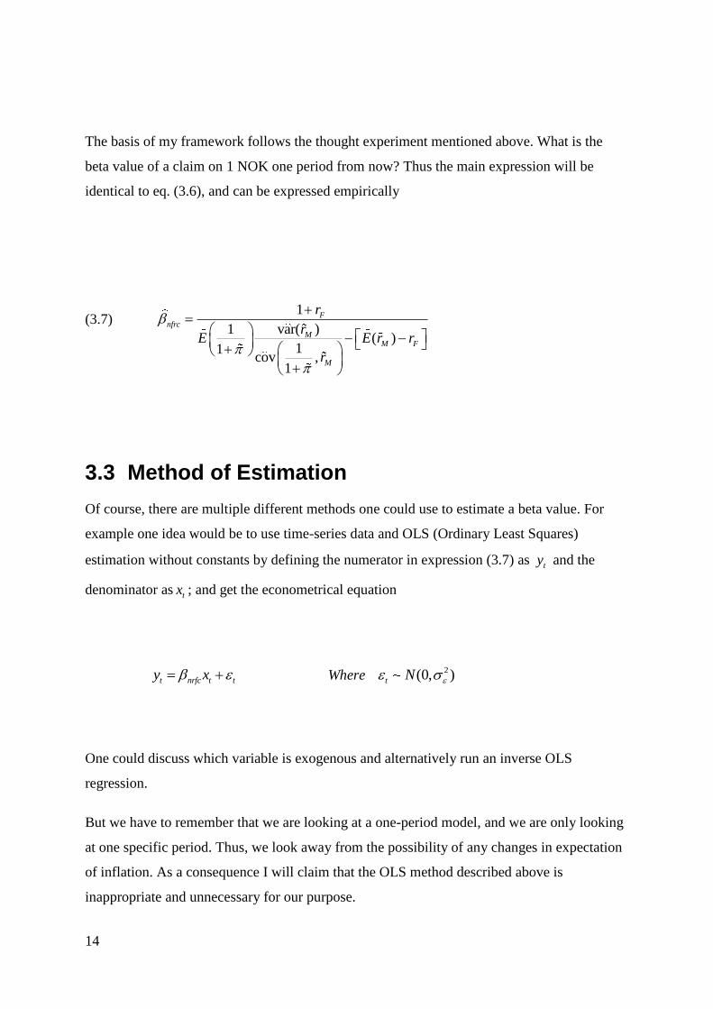
The basis of my framework follows the thought experiment mentioned above. What is the
beta value of a claim on 1 NOK one period from now? Thus the main expression will be
identical to eq. (3.6), and can be expressed empirically
(3.7) 1
var( )1( )
11cov ,
1
Fnfrc
MM F
M
r
rE E r r
r
3.3 Method of Estimation
Of course, there are multiple different methods one could use to estimate a beta value. For
example one idea would be to use time-series data and OLS (Ordinary Least Squares)
estimation without constants by defining the numerator in expression (3.7) as ty and the
denominator as tx ; and get the econometrical equation
t nrfc t ty x Where 2(0, )t N
One could discuss which variable is exogenous and alternatively run an inverse OLS
regression.
But we have to remember that we are looking at a one-period model, and we are only looking
at one specific period. Thus, we look away from the possibility of any changes in expectation
of inflation. As a consequence I will claim that the OLS method described above is
inappropriate and unnecessary for our purpose.

15
The method I will use initially is rather simple. Basically I will use time-series data from
Norway and estimate the empirical moments of the (.)E -, var(.) - and cov(.) - expressions
above and insert back into equation (3.7) to get an estimated value of beta.
A Note on Empirical Moments
Method of moments is a famous method of estimation of parameters such as mean, variance,
covariance, etc. The sth moment of a probability law is defined as
( )s
s E Y
where Y represents a random variable following the probability law. If there are n
independent and identically distributed (i.i.d.) variables, the sth sample moment is defined as
1
1ˆ
ns
s i
i
Yn
where ˆs is an estimate of s .
The population mean is also called the expectation of Y
But with time-series data, as we have in our case, it cannot be sure that the observation values
of a variable are independent. In other words it cannot be ruled out that the observations are
serially dependent in some way. For example, with high inflation in one period it is
reasonable to believe there will be “echoing” effects on inflation in the future, i.e. that
inflation will follow an autoregressive process. Of course to assume anything a priori about
the data would be a mistake, it is a statement that has to be researched and tested. Luckily we
know that the arithmetic mean of the sample is an unbiased estimator for the expectation for

16
the period we are looking at. If we assume rational expectations we can estimate the
expectation by using the realized values of the time period in question. The sample variance is
also an unbiased estimator13
,
22
1
1
1
n
S i
i
Y Yn
The following estimations of the beta value will be based on one sample with 223 monthly
values of the CPI and thus 222 values of the inflation rate, 222 values of the real market
portfolio rate and 222 values of the real risk free rate.
3.4 The Data Set
3.4.1 The OBX-index
The OBX-index is a value weighted index consisting of the twenty-five most liquid stocks on
the Oslo stock exchange. It was introduced in 1987 with the main goal of being the basis for
derivatives contracts. In other words, all stocks included in the OBX-index are tradable with
options and futures. The stocks that are included are dividend adjusted, and the index
“portfolio” is revised twice a year.
The market portfolio is in definition a portfolio that consists of all securities available in a
given market in amounts proportional to their value. It is a theoretical concept with roots in
the modern portfolio theory. Therefore the OBX-index will in this analysis serve as a proxy
for the return on the market portfolio in Norway. We have to remember that the market rate of
13
Note that the denominator is given by ( 1)n instead of n . It is called Bessell’s correction and insures that
the sample variance is an unbiased estimator.

17
return calculated using the OBX-index will be in nominal terms, so we have to use the
inflation rate to get the real rate of return.
The data used will span from January 1988 and up to July 200614
.
3.4.2 Consumer Price Index (CPI)
To calculate inflation we use the consumer price index (CPI). The CPI is a well known
economical concept; it is the index that covers the prices of consumer goods. It is normal to
distinguish between CPI and CPI-TAE. CPI-TAE is the consumer price index adjusted for
taxes and energy prices. I will use the standard CPI in my estimations.
On the Norwegian Statistics webpage there is monthly data for CPI all the way back to 1865.
To accompany the data for the OBX-index the calculation of inflation will be based on CPI
values from January year 1988 to July 2006.
3.4.3 NIBOR
NIBOR (Norwegian Inter Bank Offered Rate) is the money market rate. It is the borrowing
rate between the banks. The rate depends on the demand and supply in the money market, but
is ultimately set by the Norwegian Central Bank. On the Norwegian Central Bank webpage
there is daily data for both monthly and annual NIBOR rates from year 1986 and up until
present time are available15
. I will use from the period January 1988-July 2006. The rate is
nominal, thus we have to transform it to a real interest rate in order to fit our model. To
achieve this we use the inflation rates from the same period.
The NIBOR will be used as a proxy of the risk free rate. This is typical practice with the main
reason being that the likelihood of default is extremely low. But of course, we have to keep in
mind that “risk free rate” is a purely theoretical concept and that there are no such interest
rates that are hundred percent risk free.
14
See in appendix for the calculation of the return of the market portfolio 15
http://www.norges-bank.no/templates/article____55483.aspx

18
3.5 Results16
Using the statistical package STATA 9.2 I have attained an estimate for the beta of the
nominally risk free claim for the period January 1988- July 2006.
First, we have the present value of 1NOK:
. Summarize present_val
Variable | Obs Mean Std. Dev. Min Max
-------------+--------------------------------------------------------
present_val | 222 .997979 .00385 .9772926 1.013863
The result gives an estimate of the expected value of the present value of 1NOK
1
0.9979791
E
Second, we have the estimate of the real market rate of return:
. summarize r_M
Variable | Obs Mean Std. Dev. Min Max
-------------+--------------------------------------------------------
r_M | 222 .0047432 .0860523 -.7980653 .1999241
which gives 0.0047432Mr
Next we have the estimate for the real risk free interest rate:
. summarize r_F
Variable | Obs Mean Std. Dev. Min Max
-------------+--------------------------------------------------------
r_F | 222 .0682132 .0404159 .013621 .4022704
0.0682132Fr
16
See appendix A.3 for the estimation procedure.

19
And at last, we find the empirical covariance between the present value of 1NOK and the
market return rate:
. correlate present_val r_M
(obs=222)
| presen~l r_M
-------------+------------------
present_val | 1.0000
r_M | 0.0385 1.0000
1 1 1
co , ,1 1 1
M M Mv r corr r std std r
0.0385 0.00385 0.0860523 0.00001276
Using all the estimated parts above we get an estimate for the beta value of the nominal risk
free claim
1ˆva1
11co ,
1
Fnrfc
M
M F
M
r
r rE E r r
v r
2
1.06821320.0018435
0.08605230.997979 0.0682132 0.0047432
0.0385 0.00385 0.0860523
3.6 Discussion
The result above yields an estimated value of beta approximately equal to 0.0018435 . It can
be argued that this is a significantly small value and that consequently the risk of inflation
uncertainty does not have an effect on the expected rate of return of equity. The beta is close
20
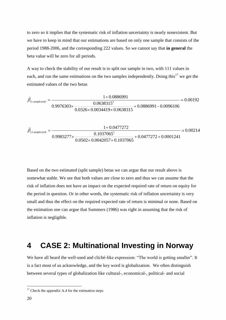
to zero so it implies that the systematic risk of inflation uncertainty is nearly nonexistent. But
we have to keep in mind that our estimations are based on only one sample that consists of the
period 1988-2006, and the corresponding 222 values. So we cannot say that in general the
beta value will be zero for all periods.
A way to check the stability of our result is to split our sample in two, with 111 values in
each, and run the same estimations on the two samples independently. Doing this17
we get the
estimated values of the two betas
(1. ) 2
1 0.08869910.00192
0.06383150.9976303 0.0886991 0.0096106
0.0326 0.0034419 0.0638315
sample nrfc
(2. ) 2
1 0.04772720.00214
0.10370650.9983277 0.0477272 0.0001241
0.0502 0.0042057 0.1037065
sample nrfc
Based on the two estimated (split sample) betas we can argue that our result above is
somewhat stable. We see that both values are close to zero and thus we can assume that the
risk of inflation does not have an impact on the expected required rate of return on equity for
the period in question. Or in other words, the systematic risk of inflation uncertainty is very
small and thus the effect on the required expected rate of return is minimal or none. Based on
the estimation one can argue that Summers (1986) was right in assuming that the risk of
inflation is negligible.
4 CASE 2: Multinational Investing in Norway
We have all heard the well-used and cliché-like expression: “The world is getting smaller”. It
is a fact most of us acknowledge, and the key word is globalization. We often distinguish
between several types of globalization like cultural-, economical-, political- and social
17
Check the appendix A.4 for the estimation steps
21
globalization. But what they all have in common is that information is transferred at high
speed, there is an increased information flow and boundaries are erased.
Of course there are different views on the globalization issue. Neo-liberalists applaud it and
argue that it brings efficiency economic prosperity while on the other side we have various
conservative nationalists who are domestically oriented and argue for a more sovereign
domestic economy.
When it comes to economical globalization isolated, an increased information flow implies
opportunities to expand and make a profit. I will in the following look from the perspective of
a U.S company that conducts an investment project in Norway. Think of it as a multinational
firm. There will be one major difference from our first case with a company investing in the
domestic market: additional to the assumed risk of inflation uncertainty there will be risk
associated with the uncertain exchange rate between Norwegian kroner and U.S dollars at the
time of conversion to U.S dollars. The U.S Company will value the depreciation deduction
according to the buying power of 1 NOK in U.S dollars. This implies that given the
depreciation deduction, which will be given in Norwegian kroner, the firm will exchange it
for USD. Since this is “business as usual” for a multinational it might thus be very interesting
to see how uncertainty of inflation will affect the required expected return of equity for the
representative firm.
4.1 The Modified Model
As mentioned, introducing exchange rates will somewhat alter the model we had in our
analysis above. But we will concentrate on a similar constellation. It is a two-period model
where the firm invests in a project in period t and in period 1t there is a tax deduction. First
we assume that the firm has a claim on 1 NOK after a given time (a depreciation deduction).
Since we are looking from the perspective of an U.S firm we have to apply data for U.S.
inflation. Namely we are looking at the present value of the buying power of 1 NOK
measured in USD,

22
(4.1) 1
1
t
USD
USD
NOK
Now, it has to be noticed that strictly speaking the nominal claim will not be risk free in this
case. The reason is that we are looking at an American company which at the date of the
future tax deduction would like to exchange the amount, which is given in NOK, to USD. But
the exchange rate one period ahead is not known so the nominal value measured in USD will
be uncertain. Luckily this is not an issue for our analysis because we are only interested in
valuing an uncertain real value, and this can be done similarly as with the first case. The
CAPM does not have any requirements that the cash flow in question has to be nominally risk
free, so the formulae that we will base our estimation on will be similar to the first case.
We can write, according to the CAPM, the value of the claim given by eq. (4.1) in period t as
(4.2) 1 1 11cov ,
1 1 1 1
t t tM
USD F USD USD
USD USD USD
NOK NOK NOKV E r
r
Equation (4.2) is analogous to equation (3.5) above.
Following the identical steps as above in case 1, we get an expression for the beta value of the
NOK-risk-free claim
(4.3)
( )
1
1
1
/ var
1 /cov ,
1
Fnrfc NOK
MtM F
USD tM
USD
r
USD NOK rE E r r
USD NOKr

23
4.2 Method of Estimation
I will use identical method as in the first case to estimate the beta value
(4.4)
( )
1
1
1
/ var
1 /cov ,
1
Fnrfc NOK
MtM F
USD tM
USD
r
USD NOK rE E r r
USD NOKr
By estimating each part, using method of moments, in eq. (4.4) and inserting back into the
expression.
4.3 The Data Set
To get an estimation of the beta value I will use data from a six-year period, 2003-2009. The
main reason is that Treasury Inflation-Protected Securities (see more below), which will be
used as a proxy for the risk free rate, was not introduced before the end of the 20th
century
(1997), and I have had some difficulties finding data for the market yield on TIPS in the
period 1997-2003. So here forth the time of the investment decision, period t , will be January
1998; and 1t , the time of depreciation deduction, will be January 2009.
4.3.1 TIPS (Treasury Inflation-Protected Securities
I have already mentioned this type of securities earlier. Basically, the U.S Treasury introduced
it in January 1997 as a means to protect investors from negative effects of inflation but also as
an instrument to reduce the interest cost to the Treasury in the long term. In the Federal
Register18
it is stated:
The Department believes the issuance of these new inflation-indexed securities will reduce the
interest costs to the Treasury over the long term and will broaden the types of debt
instruments available to investors in U.S. financial markets.
18
Department of the Treasury, Part III (January, 1997). “Sale and Issue of Marketable Book-Entry Treasury
Bills, Notes, and Bonds.” Circular, Public Debt Series No. 1-93.
24
They differ from other ordinary marketable bonds by the fact that the principal of the bonds is
constantly adjusted accordingly with inflation measured by the U.S Government. But the
interest rate, which is set at the auctions, is fixed. In other words, the principal will be fixed in
terms of purchasing power and not in terms of nominal U.S dollars. TIPS pay interest twice a
year, and since the principal varies with the inflation the interest payment will also vary.
TIPS are issued in terms of 5, 10 and 30 years. They can be hold until maturity but it is also
possible to sell them before at a secondary market. The inflation adjusted securities are sold
through TreasuryDirect, Legacy Treasury Direct, banks, dealers and brokers. The price will
depend on several factors as the yield to maturity19
and the interest rate. If the yield to
maturity, or redemption yield, is lower than the interest rate the price will be less than face
value. If it’s higher, the price will be higher than the face value and if the redemption yield is
equal to the interest rate the price will be equal to the face value.
The question of how well the treasury inflation-protected securities actually protect investors
from inflation risk has been discussed ever since the introduction of this kind of indexed
Government debt. At maturity the buyer receives the adjusted principal or the original
principal depending on which one is larger. But two main arguments stress that TIPS do not
offer perfect protection (Wilcox, 1998). The first has to do with how coupon and principal
payments are indexed to CPI. It turns out that the payments are indexed against a lagged value
of CPI, so that basically a high variation in inflation over time might cause higher risk.
The second argument involves tax treatment. More specifically, the taxable income of an
investor will not only consist of the coupon payments received during a year but also the
increase in principal induced by inflation. Thus, tax liability will rise with inflation.
An alternative to using TIPS rates as a proxy for the risk free rate is I Bonds, or I Savings
Bonds. This security type was introduced by the U.S. Government in 1998 and it offers
inflation protection to the holder, similarly as TIPS. But it can be distinguished on several
areas. For instance I Bonds operate with two rates, a fixed rate and an inflation rate. The fixed
rate is constant during the life time of the bond while the inflation rate is adjusted with
changes in the CPI and is combined with the fixed rate to get the earning rate.
19
“Yield to maturity is the interest equivalent to the actual interests payments plus capital gains (or minus capital
losses) if the security is held to maturity”, Oxford Dictionary of Economics

25
One of the major concerns of using I Bonds as a proxy for the risk free rate is that historically
they exhibit very low yield rates20
. Thus I will stick to TIPS as a proxy for risk free rate.
I have at my disposal monthly values of the historical market yield on 10-year TIPS stretching
from January 2003 to March 2010. I will base my estimations on period January 2003-
January 2009, which gives 73 values of the market yield rate.
4.3.2 Standard & Poor’s 500 (S&P 500)
Previously, when we looked at a domestic company in Norway we used the percentage
change in the OBX index as a proxy for the rate of return on the market portfolio. Now as we
look at a multinational company from the U.S. I will use the Standard & Poor’s 500 index
(S&P 500). An alternative would have been to use the Dow Jones Industrial Average. This
index is often called “Dow 30” because it contains 30 of the largest companies in the U.S. But
I will stick with the S&P 500 because it can be argued that as it includes more stocks it gives
us a broader and better description of the U.S. equity market and the economy as a whole.
The S&P 500 index was introduced in 1957 and is today regarded as the best single index for
the large cap U.S. equities market. Companies are often distinguished by their size of market
capitalization i.e. the aggregate value of the company, which is measured as the share price
times the number of shares outstanding. Large cap companies are classified by Standard &
Poor’s as companies with at least $3.5 billion market capitalization21
. The index contains the
500 most leading companies in the main U.S. industries and is set and regularly adjusted by a
committee of leading economists and index analysts. The five main criteria for index
additions are22
:
- U.S. Company: The company must be a “U.S. company” determined by the structure,
location of operation, accounting structure and its exchange listing.
- Market capitalization in excess of $3 billion: This limit can be adjusted to take into
account the market situation/conditions.
20
See table 1 of fixed rates on I Bonds in appendix C. 21
“S&P U.S. Indices: Index Methodology”, March 2010 22
http://www2.standardandpoors.com/spf/pdf/index/SP_500_Factsheet.pdf

26
- Public Float of 50%: At least 50% of the company’s shares must be tradable on the
public market.
- The company must be financially viable: It is expected that the companies included in
the index must have at least four consecutive quarters of positive (as-reported)
earnings.
- The company should have adequate liquidity and reasonable price per share: The rule
being that the ratio of annual dollar value traded to the market capitalization for the
company should be 0.30 or higher. Also shares that are priced extensively low or high
are also considered to be illiquid.
- The index must reflect the various sectors in the U.S. economy: More specifically it
means that even though a company fulfils all the criteria above it might not be chosen
to be in the index because the sector the company is a part of is already represented.
The companies included in the index are weighted based on their stock’s market value, i.e. the
S&P 500 is a market value weighted index. The main goal of the S&P Committee is to ensure
that the S&P 500 remains as the best index for U.S. equities and to serve as a tool for
assessing risk.
I have at my disposal daily values of the S&P 500 from January 2003 to January 2009. This
implies 1511 daily values. I will use a similar method as with the OBX-index to estimate the
rate of return on the market portfolio23
.
4.3.3 U.S. CPI
I will use data for the consumer price index to calculate monthly U.S inflation in the period
January 2003-January 2009. The CPI given is also denoted as CPI-U where “U” stands for
“urban”, is the most analytically used U.S. price measurement.
I have gathered data from the U.S. Department of Labour Bureau of Labour Statistics24
. I will
use monthly values of the CPI-U to calculate the monthly inflation in the U.S. The period
January 2003-January 2009 gives 72 monthly values of the inflation rate.
23
See more in appendix B. 1. 24
ftp://ftp.bls.gov/pub/special.requests/cpi/cpiai.txt

27
4.3.4 The Exchange Rate
The exchange rate measures the price of one currency in terms of another. I have data for the
exchange rate of USD measured in NOK ( /NOK USD ). This implies that USD is the base
currency and NOK is the quote currency. I have data for the monthly average exchange rate in
the period the estimation is based on (January 2003-January 2009), which gives 72 values25
.
Since we are interested in the purchasing power of 1 NOK measured in USD we have to
invert the data,
1
( / )
USD
NOK NOK USD
4.4 Results
Using data for the exchange rate and inflation we get 72 values of the present value of the
purchasing power of 1 NOK measured in USD
. summarize pre_val
Variable | Obs Mean Std. Dev. Min Max
-------------+--------------------------------------------------------
pre_val | 72 .1584073 .0161406 .1345298 .1967003
1
/0.1584073
1
t
USD
NOK USDE
25
Exchange rate data is gathered from the page http://www.norges-bank.no/templates/article____200.aspx

28
The estimated expected rate of return on the market portfolio is26
. summarize r_M
Variable | Obs Mean Std. Dev. Min Max
-------------+--------------------------------------------------------
r_M | 72 -.0018192 .0383965 -.1609489 .0833967
0.0018192ME r
Finding the empirical covariance between the purchasing power of 1NOK measured in U.S.
dollars and the rate of return on the market portfolio,
. correlate pre_val r_M
(obs=72)
| pre_val r_M
-------------+------------------
pre_val | 1.0000
r_M | -0.2188 1.0000
1 1 1
/ / /co , ,
1 1 1
t t tM M M
USD USD USD
NOK USD NOK USD NOK USDv r corr r std std r
0.2188 0.0161406 0.0383965 0.0001356
As a proxy for the risk free rate we use monthly values of the market yield rate on 10-year
TIPS:
. summarize TIPS10
Variable | Obs Mean Std. Dev. Min Max
-------------+--------------------------------------------------------
TIPS10 | 73 .020111 .0035553 .0109 .0289
which gives us 0.020111Fr .
26
See appendix B1 for a more thorough explanation

29
Inserting the empirical moments in equation (3.4) gives us the estimated beta of the NOK-
risk-free claim:
( )
1
1
1
/ var
1 /cov ,
1
Fnrfc NOK
MtM F
USD tM
USD
r
NOK USD rE E r r
NOK USDr
1.020111
0.599951.700330053
4.5 Discussion
Based on the data from the six-year period we get an estimated beta value which is negative.
This means, in pure CAPM-notion that the “return” on the NOK-risk-free claim and the return
on the market portfolio are inversely correlated. High return on the market portfolio is
accompanied with low return on the NOK-risk-free claim and vice versa.
But we cannot be surprised by the result. One argument is based on the oil price. In periods
when the oil price is varying because of supply side changes in the oil market the beta value
of the oil price will probably be negative. If the oil price is dominated by changes on the
supply side it may indicate that the general relationship between the OPEC-countries is
somewhat tense. Wars, conflicts, new technology and discovery of new oilfields are also
factors that indicate a more supply-side dominated oil price.
A higher oil price caused by the supply side will in general have two main effects on
consumers and producers respectively. First an increase in the oil price will reduce the
disposable income for consumers on other goods and services. Secondly, an increase in the oil
price will raise the costs of non-oil producing companies, inducing lower profit margins and
reduced dividends. Since profits and dividends are two of the main driving forces of stock
prices this would just as well imply lower S&P 500 index, and thus a lower rate of return on
the market portfolio.

30
If the demand side dictates, or is the leading factor of uncertainty of the oil price, the effect
will be the opposite; namely good times and optimism in the U.S. economy and the world
economy as a whole leads to increased demand for oil and therefore a higher price. Thus
higher oil price will go hand in hand with higher return on the market portfolio, implying a
positive beta value for the price of oil.
Theoretically, it is a well known belief that the value of the currency of an oil-exporting
country is positively correlated with the oil price (Golub, 1983; Corden, 1984)27
. Since
Norway is one of the major oil-exporting countries it is reasonable to believe that the value of
NOK in terms of USD is highly dependable on the oil price, i.e. the oil price has been a
dominant factor for the NOK even though the relationship has been less clear in recent years.
It is undeniable that the period 2003-2009, which I have used to estimate the beta value, has
in general been a period dominated by wars, conflicts and economic instability in the world.
Correspondingly the oil price has oscillated greatly, and reached record high levels28
. This
could in our case explain the uncertainty of NOK from the point of view of the American
multinational, with a negative beta value of the exchange rate of NOK. Of course, following
the argument above it seems that the result we get depends highly on the time period used in
estimation. One cannot deny that there is a possibility that the beta value could be positive in
a situation where the supply side is more stable.
5 Concluding Remarks
Above we first looked at the beta value of a nominally risk free claim for a domestic company
in Norway. Further on we continued with an American multinational with an investment
project in Norway. In the first case we used data in the time period 1988-2006 while in the
second case we used data from a more narrow time period, 2003-2009. The results can be
summarized in a table:
27
There are some empirical studies that when it comes to Norway contradict this linear relationship, see Akram
(2002). He uses the NOK/ECU exchange rate. 28
See chart 2 in appendix C.

31
CASES
CASE 1: Domestic Firm in Norway 0.0018435nrfc
CASE 1 (1st split sample) (1. ) 0.00192sample nrfc
CASE 1 (2nd split sample) (2. ) 0.00214sample nrfc
CASE 2: U.S. Multinational in Norway ( ) 0.59995nrfc NOK
Lund (2002) found in the case with certain tax position that the beta value of the future net
cash flow would be lower than the beta value of the uncertain price P , as long as the tax
system does not imply a pure cash flow tax or Brown tax as often called. The main argument
is that the depreciation schedules act as loan from the firm to the Government. Since in this
case the probability of “default” in is non-existent, meaning that the deprecation allowance is
a certain future cash flow for the firm, the risk of equity would be reduced.
When we introduced the potential risk of inflation uncertainty we got a beta value of the
nominally risk-free cash flow close to zero. This would indicate that the inflation risk does not
add to the risk of the future net cash flow of the firm. With this result one could defend the
statement by Summers (1986) who argued that the risk of depreciation allowances are
“nearly” risk-free. But it has to be noted that only one period has been used in the estimation
of the beta value. Therefore we cannot be sure that the beta value of the nominally risk-free
claim will be similar for other periods with a different economic situation.
In the second case we found a negative beta value of the NOK-risk-free claim. This implies
that the beta of the after-tax net cash flow would be lower than in Lund (2002) where
uncertainty of inflation risk was not included. I argued that the oil price has a great impact on
the value of NOK, and thus the uncertainty of the exchange rate from the point of view of the
American multinational. Variations in the oil price in the period I looked at were heavily
influenced by the supply side. This could explain the negative value of our result.
What can we conclude based on these results? Well, the estimations did not give us any clear
answers about whether inflation uncertainty risk, in general, is an important factor in

32
valuation of future real cash flows. But I will claim that it gives us a quite clear example that
valuing a future real cash flow will depend on the period and from which perspective the
analysis is based on.

33
References
Akram, Q. F. (2002). ”Oil Prices and Exchange Rates: Norwegian Evidence.” In
Econometrics Journal, 2004, Vol. 7, pages 476-504.
Corden, W. M. (1984). “Booming Sector and Dutch Disease Economics: Survey and
Consolidation.” In Oxford Economic Papers, 36, 1984, pages 359-380.
Golub, S. S. (1983). “Oil Prices and Exchange Rates.” In The Economical Journal, Vol. 93,
No. 371 (Sep., 1983), pages 576-593.
Karlsson & Nordén. (2007). “Home Sweet Home: Home Bias and International
Diversification among Individual Investors.” In
Lintner, J. (1965a.) “The Valuation of Risk Assets and the Selection of Risky Investments in
Stock Portfolios and Capital Budgets.” In Review of Economics and Statistics, No. 4, pages
13-37.
Lintner, J. (1965b.) “Security Prices, Risk and Maximal Gains from Diversification.” In
Journal of Finance, No. 20, pages 587-615.
Lund, D. (2002). “Taxation, Uncertainty, and the Cost of Equity.” In International Tax and
Public Finance, 9, pages 483-503.
Lund, D. (2009). “Marginal versus Average Beta of Equity under Corporate Taxation”
Mossin, J. (1966). “Equilibrium in a Capital Asset Market.” In Econometrica, No. 35, pages
768-783.
Perold, A.F. (2004). “The Capital Asset Pricing Model.” In The Journal of Economic
Perspectives, Vol. 3, No. 3, pages 3-24.
Ruback, R.S. (1986) “Calculating the Market Value of Riskless Cash Flows.” In the Journal
of Financial Economics.
Sharpe, W. F. (1964). “Capital Asset Prices: A Theory of Market Equilibrium under
Conditions of Risk”. In The Journal of Finance, Vol. 19, No. 3, pages 425-442.

34
Summers, L. H. (1986). “Incentives and the Discounting of Depreciation Allowances.” In M.
Feldstein (ed.), The Effects of Taxation on Capital Accumulation. Chicago: University of
Chicago Press.
Treynor, J. L. (1962). “Toward a Theory of Market Value of Risky Assets.” Final version in
Asset Pricing and Portfolio Performance, 1999, Robert A. Korajczyk, ed., London: Risk
Books, pages 15-22.
Wilcox, D.W, (1998). “The Introduction of Indexed Government Debt in the United States.”
In The Journal of Economic Perspectives, Vol. 12, No. 1, pages 219-227.
Ødegaard, B. A. (2009). “Empirics of the Oslo Stock Exchange. Basic, descriptive, results.”
From webpage:
http://www1.uis.no/ansatt/odegaard/wps/empirics_ose_basics/empirics_ose_basics_aug_2009
.pdf , Pedagogical Working Paper.
“Real Beskatting: betänkande” by Realbeskattningsutredningen, 1-3 (1982), Stockholm:
Liber.
Department of the Treasury, Part III (January, 1997). “Sale and Issue of Marketable Book-
Entry Treasury Bills, Notes, and Bonds.” Circular, Public Debt Series No. 1-93.
S&P U.S. Indices: Index Methodology:
http://www2.standardandpoors.com/spf/pdf/index/SP_US_Indices_Methodology_Web.pdf
U.S Department of the Treasury: TIPS in Depth,
http://www.treasurydirect.gov/indiv/research/indepth/tips/res_tips.htm
Norges Bank: NIBOR, http://www.norges-bank.no/templates/article____55483.aspx,
downloaded 12.02.2010.
Standard & Poor’s: S&P 500,
http://www2.standardandpoors.com/spf/pdf/index/SP_500_Factsheet.pdf, downloaded
02.03.2010.

35
Data for the OBX-index gathered from the data source NHH’s Børsprosjektet:
http://www.mora.rente.nhh.no/borsprosjektet/default.aspx, access gained from Oslo Børs on
21.01.2010.
Monthly data on NIBOR rates: http://www.norges-bank.no/templates/article____55483.aspx ,
downloaded on 03.02.2010.
Monthly data on the market yield for
TIPS:http://www.federalreserve.gov/releases/h15/data/Monthly/H15_TCMII_Y10.txt,
downloaded on 15.03.2010
Monthly average exchange rate: http://www.norges-bank.no/templates/article____200.aspx,
downloaded 05.03.2010
U.S. CPI-U: ftp://ftp.bls.gov/pub/special.requests/cpi/cpiai.txt , downloaded 05.03.2010

36
6 Appendix
6.1 Appendix A
A.1:FINDING EQ. (3.4)
We have equation
(3.3)
cov ,( )
var( )
M
P
M
Pr
V P
r
Inserting the expression for ( )V P we get,
cov ,1
( ) cov( , )1
var( )
M
M
F
P
M
Pr
E P P rr
r
(1 )
cov ,( )
( ) cov( , )var( )
var( )
FM
M F
M
M
M
P rr
E r rE P P r
r
r
(1 ) var( )cov ,
( ) var( ) ( ) cov( , )
var( )
F MM
M M F M
M
P r rr
E P r E r r P r
r

37
(1 )cov ,
( ) var( ) ( ) cov( , )
FM
M M F M
P rr
E P r E r r P r
Since we assume that Fr is a given (constant) and known, we can write
(1 )cov ,( ) var( ) ( ) cov( , )
P F M
M M F M
Pr r
E P r E r r P r
cov ,(1 )
( ) var( ) ( ) cov ,
M
F
M M F M
P rr
E P r E r r P r
this simplifies to equation (3.4):
(3.4)
1
var( )( ) ( )
cov( , )
FP
MM F
M
r
rE P E r r
P r
A.2: FINDING EQ. (3.6)
To get eq. (3.6) we use analogous steps as we used finding eq. (3.4). We start up with the
expression of the beta value
1/ (1 )cov ,
1/1
var( )
M
nrfc
M
rV
r

38
Following the same steps as above will give us the expression of the beta of the nominally
risk free claim,
(3.6)
1
var( )1
11cov ,
1
Fnrfc
MM F
M
r
rE E r r
r
A.3:Estimation Procedure
Calculating Market Rate of Return
I have 4658 daily values of the OBX-index from the time period 04.01.1988-03.07.2006.
From these data I extract the value for the first day in each month, which gives me 223 values.
In order to get an estimate of the market rate of return I first calculate the relative change in
the OBX-index for each month. These values are then multiplied with their respective factors
which take into account our assumption that a month contains 30 days. Mathematically we
can express
1
1
30
.
t tm t
t
OBX OBXr
OBX no days
where .no days is the number of days between the between the two values. With this procedure
we get 222 values of the market rate of return. Alternatively, we could have used a
logarithmic approximation
1
1 1
30 30ln
. .
t t t
t t
OBX OBX OBX
OBX no days OBX no days

39
The real market portfolio rate can be mathematically defined as
1
11 1
m mM M
r rr r
To find the expected market rate of return we simply calculate the mean:
222
222
M tt
M
r
E r
Calculating Inflation
From Norway Statistics we obtain monthly CPI data from January 1988 to July 2006, which
gives 223 values. Calculating monthly inflation is straightforward and can be expressed as
1
1
t tt
t
CPI CPI
CPI
Similarly as the market rate of return, we get 222 values of the inflation rate.
Risk free interest rate
As mentioned we use the NIBOR rate as a proxy for the risk free interest rate. The values
used is the first rate in each month of the monthly NIBOR rate in the period January 1988-
July 2006. The data we have gives us the nominal NIBOR rate. For our purpose we have to
calculate/estimate the real interest rate. The real interest rate can be defined as

40
1
11 1
f f
F F
r rr r
Using the data for inflation over the specified period gives 222 values of the real risk free
interest rate. This will serve as our data for the real risk free interest rate.
Expected present value of 1 NOK
We already have 222 value of the inflation rate. Thus, we also have 222 values of the present
value of 1 NOK,1/ (1 ) . To estimate the expected value, we simply calculate the mean of
our data
2221 1 1
1 222 1t t
E
Covariance
In order to estimate the covariance between the present value of one 1NOK and the market
rate of return, we use the empirical moment
2221 1 1 1
,1 222 1 1
M M Mtt t
cov r E r E r

41
A. 4: Checking the Stability of Estimation (Split Sample)
As we saw in the results above the estimated value of the beta was quite small. A way to
check the stability of our estimation, as mentioned, is to split the sample in two and run the
same estimation method on both samples.
Our sample consists of 223 values. We start with splitting the sample in two with 111
observations in each sample. The first sample includes data from January year 1988 to April
1997 while the second sample includes data from May 1997 to July 2006.
Sample 1:
The present value of 1 NOK:
. summarize present_val
Variable | Obs Mean Std. Dev. Min Max
-------------+--------------------------------------------------------
present_va~e | 111 .9976303 .0034419 .9855831 1.005314
10.9976303
1E
The estimate of the real market rate of return:
. summarize r_M
Variable | Obs Mean Std. Dev. Min Max
-------------+--------------------------------------------------------
r_M1 | 111 .0096106 .0638315 -.2081884 .1648269
( ) 0.0096106ME r
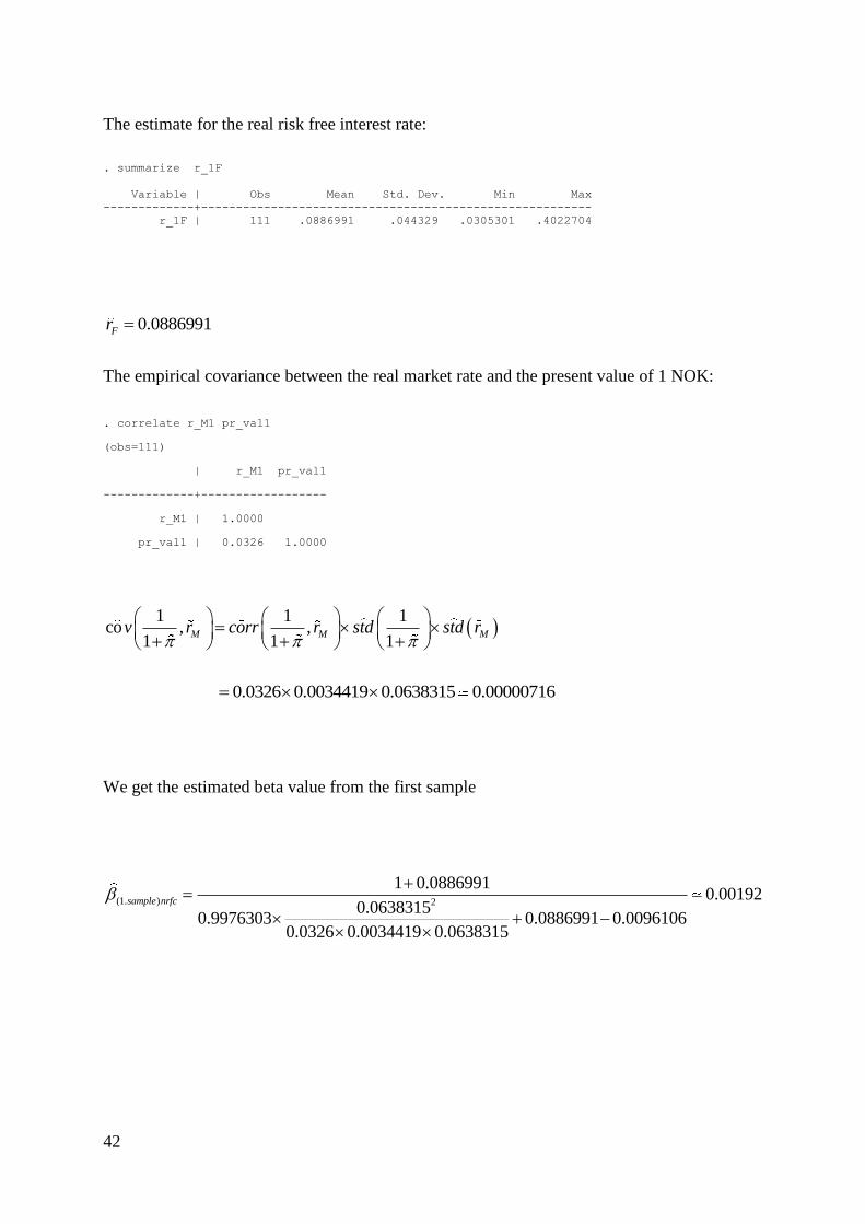
42
The estimate for the real risk free interest rate:
. summarize r_1F
Variable | Obs Mean Std. Dev. Min Max
-------------+--------------------------------------------------------
r_1F | 111 .0886991 .044329 .0305301 .4022704
0.0886991Fr
The empirical covariance between the real market rate and the present value of 1 NOK:
. correlate r_M1 pr_val1
(obs=111)
| r_M1 pr_val1
-------------+------------------
r_M1 | 1.0000
pr_val1 | 0.0326 1.0000
1 1 1
co , ,1 1 1
M M Mv r corr r std std r
0.0326 0.0034419 0.0638315 0.00000716
We get the estimated beta value from the first sample
(1. ) 2
1 0.08869910.00192
0.06383150.9976303 0.0886991 0.0096106
0.0326 0.0034419 0.0638315
sample nrfc

43
Sample 2:
Present value of 1NOK
. summarize pr_val2
Variable | Obs Mean Std. Dev. Min Max
-------------+--------------------------------------------------------
present_va~e | 111 .9983277 .0042057 .9772926 1.013863
10.9983277
1E
The estimate of the real market rate of return:
. summarize r_M2
Variable | Obs Mean Std. Dev. Min Max
-------------+--------------------------------------------------------
r_M2 | 111 -.0001241 .1037065 -.7980653 .1999241
( ) 0.0001241ME r
The estimate of the real risk free interest rate:
. summarize r_F2
Variable | Obs Mean Std. Dev. Min Max
-------------+--------------------------------------------------------
r_2F | 111 .0477272 .0216727 .013621 .0881794
0.0477272Fr
The empirical covariance:
. correlate pr_val2 r_M2
(obs=111)
| pr_val2 r_M2
-------------+------------------
pr_val2 | 1.0000
r_M2 | 0.0502 1.0000

44
1 1 1
co , ,1 1 1
M M Mv r corr r std std r
0.0502 0.0042057 0.1037065 0.0000219
The estimated beta value from the second sample
(2. ) 2
1 0.04772720.00214
0.10370650.9983277 0.0477272 0.0001241
0.0502 0.0042057 0.1037065
sample nrfc
6.2 Appendix B
B.1: Finding the Rate of Return on the market portfolio
We have, as mentioned above, 1511 historical values of the S&P 500 index. In order to use
the index as a proxy for the rate of return on the market portfolio we first extract the first price
in each month to get the monthly values. Then we find the percentage change between each
month and multiply with, similarly as we did in the 1st case with the OBX-index, the factor
that takes into account the number of days between each value:
1
1
30
.
t tm t
t
SPX SPXr
SPX no days
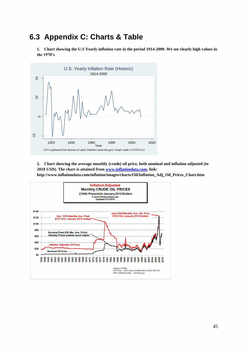
45
6.3 Appendix C: Charts & Table
1. Chart showing the U.S Yearly inflation rate in the period 1914-2009. We see clearly high values in
the 1970’s
2. Chart showing the average monthly (crude) oil price, both nominal and inflation adjusted (in
2010 USD). The chart is attained from www.inflationdata.com, link:
http://www.inflationdata.com/inflation/images/charts/Oil/Inflation_Adj_Oil_Prices_Chart.htm
-10
01
02
0
Infla
tion
(%
)
1920 1940 1960 1980 2000 2020Year
CPI-U gathered from Bureau of Labor Statistics (www.bls.gov). Graph made in STATA 9.2
1914-2009
U.S. Yearly Inflation Rate (Historic)
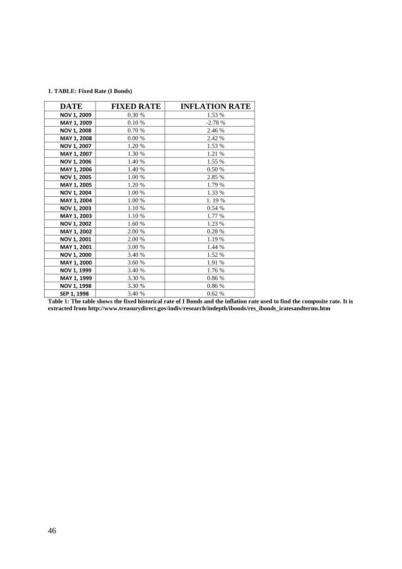
46
1. TABLE: Fixed Rate (I Bonds)
DATE FIXED RATE INFLATION RATE NOV 1, 2009 0.30 % 1.53 %
MAY 1, 2009 0.10 % -2.78 %
NOV 1, 2008 0.70 % 2.46 %
MAY 1, 2008 0.00 % 2.42 %
NOV 1, 2007 1.20 % 1.53 %
MAY 1, 2007 1.30 % 1.21 %
NOV 1, 2006 1.40 % 1.55 %
MAY 1, 2006 1.40 % 0.50 %
NOV 1, 2005 1.00 % 2.85 %
MAY 1, 2005 1.20 % 1.79 %
NOV 1, 2004 1.00 % 1.33 %
MAY 1, 2004 1.00 % 1. 19 %
NOV 1, 2003 1.10 % 0.54 %
MAY 1, 2003 1.10 % 1.77 %
NOV 1, 2002 1.60 % 1.23 %
MAY 1, 2002 2.00 % 0.28 %
NOV 1, 2001 2.00 % 1.19 %
MAY 1, 2001 3.00 % 1.44 %
NOV 1, 2000 3.40 % 1.52 %
MAY 1, 2000 3.60 % 1.91 %
NOV 1, 1999 3.40 % 1.76 %
MAY 1, 1999 3.30 % 0.86 %
NOV 1, 1998 3.30 % 0.86 %
SEP 1, 1998 3.40 % 0.62 %
Table 1: The table shows the fixed historical rate of I Bonds and the inflation rate used to find the composite rate. It is
extracted from http://www.treasurydirect.gov/indiv/research/indepth/ibonds/res_ibonds_iratesandterms.htm