Embed Size (px)
Citation preview
Gauge Institute H. Vic Dannon and Vadim Komkov
Infinitesimal Elasticity, Variational Principles, and
Castigliano Theorems [email protected] 1918-2008
H. Vic Dannon and Vadim Komkov
February, 2012
Abstract The Equilibrium Equations of Elasticity are
never derived as Euler’s Variational Equations. A
Hamiltonian is not identified in Elasticity, and Hamilton’s
Equations are absent from Elasticity Theory.
Elasticity Theory includes Variational Principles known as
Castigliano Theorems. Do the Castigliano Theorems of
Elasticity Theory stem from Variational Principles that are
unknown in Mechanics?
We show that Castigliano’s Theorems are equivalent to
Euler’s Variational Equations, and to Hamilton’s Variational
Equations.
To that end we had to set up the theory of elasticity with
infinitesimals, and give proofs to fundamental theorems of
elasticity we found unproven.
1
Gauge Institute H. Vic Dannon and Vadim Komkov
The incomplete analysis that left Elasticity Theorems
unproven, was not helped by concern about tensors in
several Elasticity texts. For the sake of clarity, we avoided
proofs with tensor indices here.
Keywords: Infinitesimal, Variation, Euler’s Variational
Equation, Variational Calculus, Variational Derivative,
Legendre Sufficient Condition, Elasticity, Stress, Strain,
Energy, Castigliano, Beam Bending, Shear.
2000 Mathematics Subject Classification; 49-02;26E30;
26E15; 26E20; 26A12; 46S20; 97I40;
Physics and Astronomy Classification Scheme
;45.20.Jj; 4510Db;
2
Gauge Institute H. Vic Dannon and Vadim Komkov
Contents
Introduction 1. Hyper-real Line
2. Strain and Stress on a Bar
3. Strain Energy of a Bar
4. Variational principles of a Bar
5. Strain on a Plate
6. Stress on a Plate
7. Strain Energy of a Plate
8. Variational principles on a Plate
9. Strain on a Box
10. Stress on a Box
11. Strain Energy of a Box
12. Variational Principles on a Box
13. Castigliano Theorems
14. Erroneous Derivations of Castigliano Theorems
15. Castigliano Theorems and the Principle of Virtual Work
16. Castigliano Theorems and the Hamiltonian
17. Castigliano and Beam Bending without Shear
References
3
Gauge Institute H. Vic Dannon and Vadim Komkov
Introduction
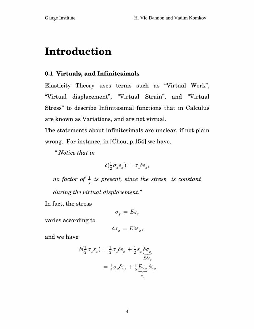
0.1 Virtuals, and Infinitesimals
Elasticity Theory uses terms such as “Virtual Work”,
“Virtual displacement”, “Virtual Strain”, and “Virtual
Stress” to describe Infinitesimal functions that in Calculus
are known as Variations, and are not virtual.
The statements about infinitesimals are unclear, if not plain
wrong. For instance, in [Chou, p.154] we have,
“ Notice that in
12
( )x x x xδ σ ε σ δε= ,
no factor of 12
is present, since the stress is constant
during the virtual displacement.”
In fact, the stress
x xEσ ε= varies according to
x xEδσ δε= , and we have
1 1 12 2 2
( )
x
x x x x x x
Eδε
δ σ ε σ δε ε δσ= +
1 12 2
x
x x x xE
σ
σ δε ε δε= +
4
Gauge Institute H. Vic Dannon and Vadim Komkov
. x xσ δε=
0.2 Infinitesimals and Limits
In terms of the Calculus of Limits, Stress is defined by
0limA
PAΔ →
ΔΔ
,
where is the force on the area . PΔ AΔ
It is difficult to imagine what this limit amounts to when
. 0AΔ →
It is easier to comprehend the quotient
dPdA
,
where the infinitesimal dA is always positive, and never
vanishes.
To avoid the fogginess of limits in Calculus, we have to use
infinitesimals.
0.3 The Strain Energy
The reason why the infinitesimal strain energy density for a
bar is
x xd dμ σ ε= ,
is beyond all texts. The text by [Timoshenko] supplies only a
5
Gauge Institute H. Vic Dannon and Vadim Komkov
plausibility argument for it.
It is even less obvious why the infinitesimal strain energy
density of a plate is
2xx xx xy xy yy yyd d d dμ σ ε σ ε σ ε= + + .
Then, without any explanation, texts conclude that
1 12 2xx xx xy xy yy yyμ σ ε σ ε σ ε= + + ,
leaving unexplained the fact that the strain in the x
direction on a plate depends on the stress in the y direction.
0.4 Variational Principles of Elasticity
The Principle of Virtual Work, and the Principle of Minimal
Potential Energy at Equilibrium, are stand-alones,
disconnected from mainstream Variational Principles of
Mechanics.
The Principle of Virtual Work is equivalent to Elasticity’s
Equilibrium equations, which are hinted to be Euler’s
Variational Equations. But are never derived from Euler’s
Variational Theory.
The Principle of Minimal Potential Energy can be
established only with the Calculus of Variations. But
Variations are alien to Elasticity Theory.
6
Gauge Institute H. Vic Dannon and Vadim Komkov
Weinstock [Weinstock, pp. 199-260] derives the equations of
Equilibrium in order to discuss transverse vibrations of bars,
and plates. But once the kinematics is eliminated from his
derivation, the Elasticity of structures remains, where
Hooke’s law is replaced by ( )f x k= x , and a body is replaced
by its center of mass.
0.5 Castigliano Theorems, and Hamilton's Equations
A Hamiltonian is not identified in Elasticity, and Hamilton’s
Equations are absent from Elasticity Theory.
Elasticity Theory of Structures includes Variational
Principles known as Castigliano Theorems.
Do the Castigliano Theorems stem from Variational
Principles that are unknown in Mechanics?
We show that Castigliano’s Theorems are equivalent to
Euler’s Variational Equations, and to Hamilton’s Variational
Equations.
7
Gauge Institute H. Vic Dannon and Vadim Komkov
1.
Hyper-real Line Each real number α can be represented by a Cauchy
sequence of rational numbers, so that . 1 2 3( , , ,...)r r r nr α→
The constant sequence ( is a constant hyper-real. , , ,...)α α α
In [Dan1] we established that,
1. Any totally ordered set of positive, monotonically
decreasing to zero sequences constitutes a
family of infinitesimal hyper-reals.
1 2 3( , , ,...)ι ι ι
2. The infinitesimals are smaller than any real number,
yet strictly greater than zero.
3. Their reciprocals (1 2 3
1 1 1, , ,...ι ι ι ) are the infinite hyper-
reals.
4. The infinite hyper-reals are greater than any real
number, yet strictly smaller than infinity.
5. The infinite hyper-reals with negative signs are
smaller than any real number, yet strictly greater than
. −∞
6. The sum of a real number with an infinitesimal is a
8
Gauge Institute H. Vic Dannon and Vadim Komkov
non-constant hyper-real.
7. The Hyper-reals are the totality of constant hyper-
reals, a family of infinitesimals, a family of
infinitesimals with negative sign, a family of infinite
hyper-reals, a family of infinite hyper-reals with
negative sign, and non-constant hyper-reals.
8. The hyper-reals are totally ordered, and aligned along
a line: the Hyper-real Line.
9. That line includes the real numbers separated by the
non-constant hyper-reals. Each real number is the
center of an interval of hyper-reals, that includes no
other real number.
10. In particular, zero is separated from any positive
real by the infinitesimals, and from any negative real
by the infinitesimals with negative signs, . dx−
11. Zero is not an infinitesimal, because zero is not
strictly greater than zero.
12. We do not add infinity to the hyper-real line.
13. The infinitesimals, the infinitesimals with
negative signs, the infinite hyper-reals, and the infinite
hyper-reals with negative signs are semi-groups with
9
Gauge Institute H. Vic Dannon and Vadim Komkov
respect to addition. Neither set includes zero.
14. The hyper-real line is embedded in , and is
not homeomorphic to the real line. There is no bi-
continuous one-one mapping from the hyper-real onto
the real line.
∞
15. In particular, there are no points on the real line
that can be assigned uniquely to the infinitesimal
hyper-reals, or to the infinite hyper-reals, or to the non-
constant hyper-reals.
16. No neighbourhood of a hyper-real is
homeomorphic to an ball. Therefore, the hyper-
real line is not a manifold.
n
17. The hyper-real line is totally ordered like a line,
but it is not spanned by one element, and it is not one-
dimensional.
10
Gauge Institute H. Vic Dannon and Vadim Komkov
2.
Strain, and Stress on a Bar
2.1 Strain-Displacement Relation for a Bar
2 2( ') ( ) 2dx dx dxdu− ≈
2 '( )
x
dx u x dxε
= .
The x -gradient of the displacement is the Axial Strain
elongation per unit length inx direction. ,x xuε ≡ =
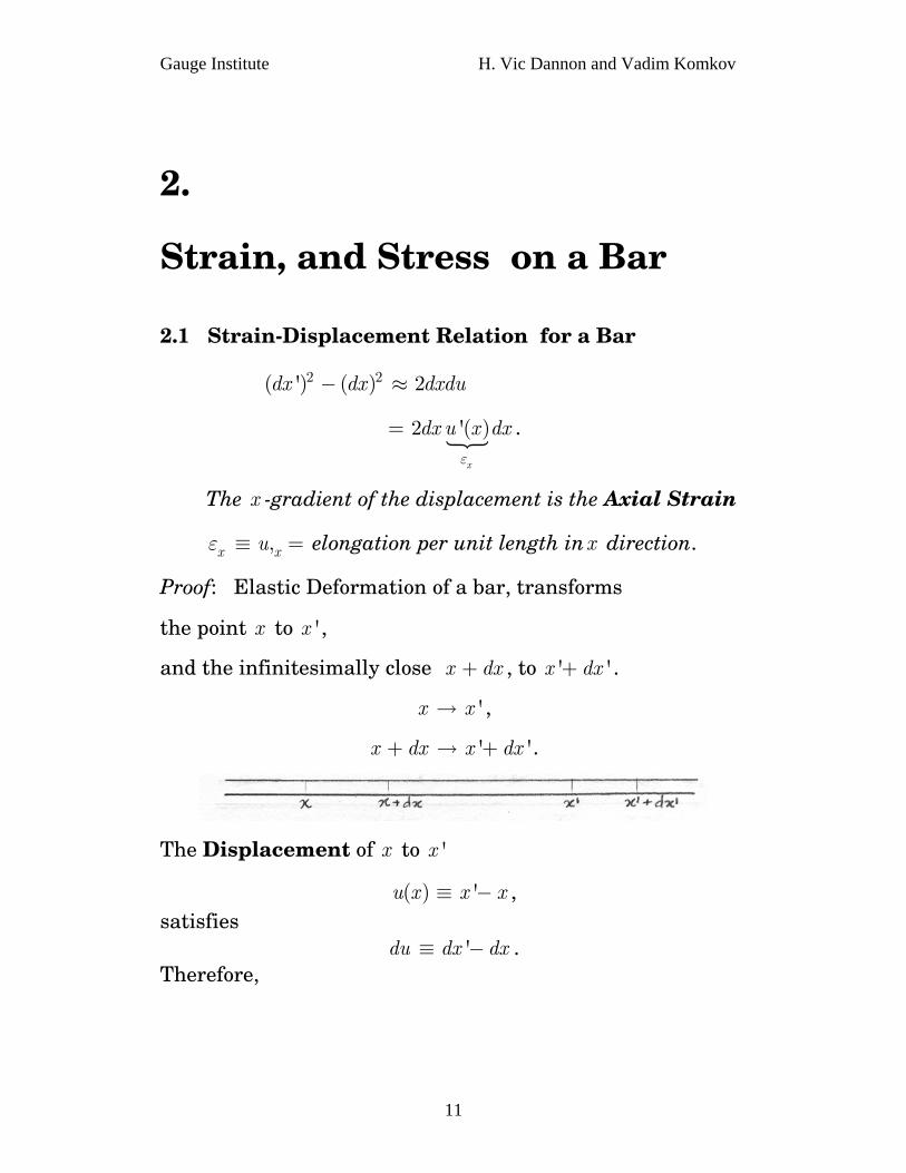
Proof: Elastic Deformation of a bar, transforms
the point x to , 'x
and the infinitesimally close x , to . dx+ ' 'x dx+
'x x→ ,
' 'x dx x dx+ → + .
The Displacement of x to 'x
( ) 'u x x x≡ − , satisfies
'du dx dx≡ − . Therefore,
11

Gauge Institute H. Vic Dannon and Vadim Komkov
2 2' ' ( ) ( )dx dx dxdx dx du dx− = + −
2dxdu dudu= +
Keeping first order in du , we have,
2dxdu≈
. ,
2( ) '( )( )
xu
dx u x dx=
And is approximated by . 2( ) (dx du dx+ − 2) 2( ) ( )xdx dxε
2.2 The Axial Stress xσ
The Axial Stress is the force stretching the bar per
unit area of the bar’s cross section.
( )x xσ
2.3 Hook’s Law, Stress-Strain Relation in a Bar
The strain and the stress satisfy Hooke’s Law
x xEσ ε≡ ,
where the Young Modulus is a constant that
characterizes the Elastic material.
E
2.4 Body Force on a Bar ( )xf x
12
Gauge Institute H. Vic Dannon and Vadim Komkov
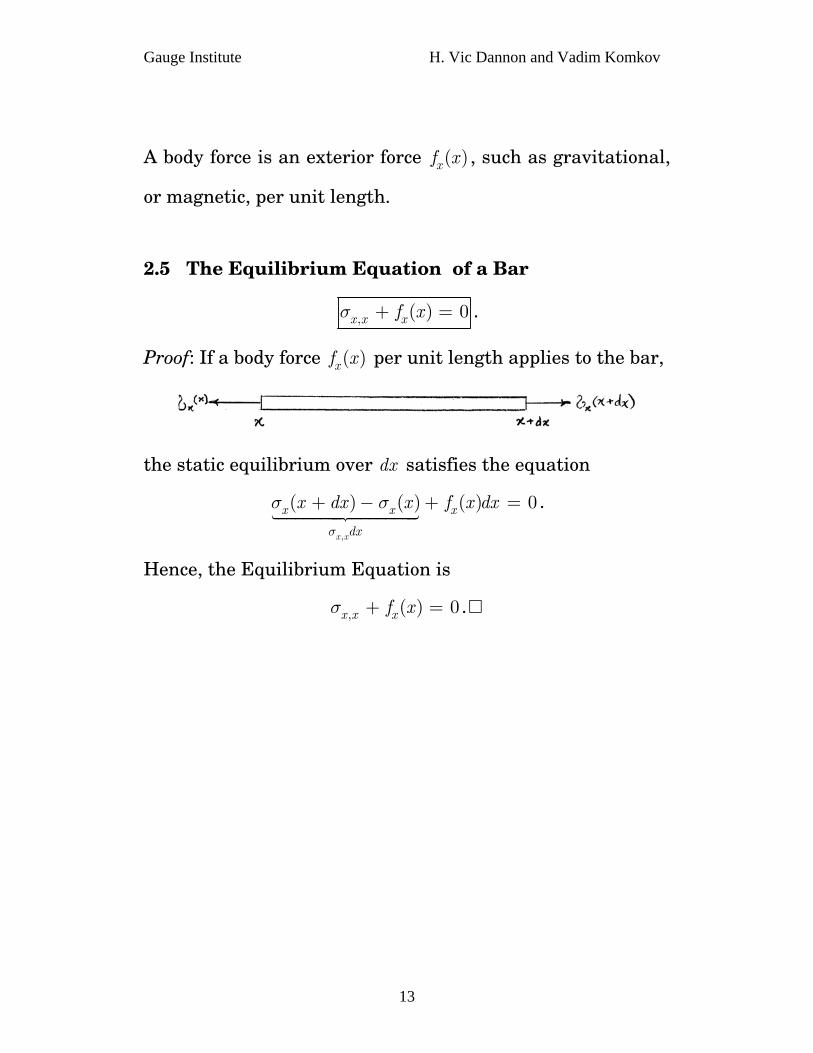
A body force is an exterior force ( )xf x , such as gravitational,
or magnetic, per unit length.
2.5 The Equilibrium Equation of a Bar
, ( ) 0x x xf xσ + = .
Proof: If a body force ( )xf x per unit length applies to the bar,
the static equilibrium over dx satisfies the equation
,
( ) ( ) ( ) 0
x x
x x x
dx
x dx x f x dx
σ
σ σ+ − + = .
Hence, the Equilibrium Equation is
, ( ) 0x x xf xσ + = .
13
Gauge Institute H. Vic Dannon and Vadim Komkov
3.
Strain Energy of a Bar
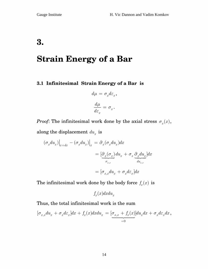
3.1 Infinitesimal Strain Energy of a Bar is
x xd dμ σ ε= ,
xx
ddμ
σε
= .
Proof: The infinitesimal work done by the axial stress ,
along the displacement is
( )x xσ
xdu
( ) ( ) ( )x x x x x x xx dx xdu du du dxσ σ σ
+− = ∂
, ,
[ ( ) ]
x x x x
x x x x x x
du
du du dx
σ
σ σ= ∂ + ∂
,[ ]x x x x xdu d dxσ σ ε= +
The infinitesimal work done by the body force ( )xf x is
( )x xf x dxdu
Thus, the total infinitesimal work is the sum
, ,
0
[ ] ( ) [ ( )]x x x x x x x x x x x x xdu d dx f x dxdu f x du dx d dxσ σ ε σ σ ε
=
+ + = + + ,
14

Gauge Institute H. Vic Dannon and Vadim Komkov
x xd dxσ ε=
The Infinitesimal work is stored in the bar as Strain Energy.
The Infinitesimal Axial Strain Energy per unit length is
x xd dμ σ ε= . That is,
xx
ddμ
σε
= .
3.2 Axial Strain Energy density of a Bar is
212 xEμ ε= .
Proof:
212
( )x x x x xd d E d Edμ σ ε ε ε ε= = =
212 xEμ ε= .
3.3 Complementary Axial Strain Energy of a Bar is
212 xE
μ σ∗ = ,
xx
ddμ
εσ
∗= .
Proof: The complementary axial strain energy density is the
axial strain energy density expressed in terms of the stress.
15
Gauge Institute H. Vic Dannon and Vadim Komkov
by substituting 1x xEε = σ into μ , we obtain
212 xE
μ σ∗ = .
Although equals , it is denoted by μ to specify its
dependence on the stress.
μ∗ μ ∗
Differentiating both sides,
1
x
x xEd d
ε
μ σ∗ = σ .
xx
ddμ
εσ
∗= .
16
Gauge Institute H. Vic Dannon and Vadim Komkov
4.
Variational Principles of a Bar
4.1 Euler’s Variational Equation
The deflection u that minimize or maximizes the Bar’s
energy per unit length,
( , , ')F F x u u=
satisfies Euler’s Variational Equation
( , , ') 0F x u uδ = ,
which is,
0'
F d Fu
u dx uδ
⎛ ⎞∂ ∂ ⎟⎜ − =⎟⎜ ⎟⎟⎜ ∂ ∂⎝ ⎠.
or,
0'
F d Fu dx u
∂ ∂− =
∂ ∂.
Proof: The Bar’s infinitesimal energy is 12
12
( , ( ), '( )
x dx
x dx
F u u d
ξ
ξ
ξ ξ ξ= +
= −∫ ξ .
The deflection u that minimizes or maximizes the bar’s
energy satisfies Euler’s Variational Equation
( , , ') 0F x u uδ = .
17

Gauge Institute H. Vic Dannon and Vadim Komkov
That is,
' 0'x
xx D u
F Fu u
u u δ
δ δ∂ ∂
+ =∂ ∂
.
Integration by parts, where vanishes on the boundary,
[Dan3] leads to the variational equation
uδ
0'
F d Fu
u dx uδ
⎛ ⎞∂ ∂ ⎟⎜ − =⎟⎜ ⎟⎟⎜ ∂ ∂⎝ ⎠.
Since this holds for any variation , the deflection u , that
minimizes or maximizes the bar’s energy satisfies Euler’s
uδ
Equation
'F d Fu dx u
∂ ∂−
∂ ∂.
4.2 If the body forces originate from a Potential per ( )uυ
unit length, so that
xfuυ∂
− =∂
Then, Euler’s Equation is the Equilibrium Equation
, 0x x xfσ + = .
Proof: The Energy per unit length is
( , ( ), '( ))F x u x u x μ υ= +
18
Gauge Institute H. Vic Dannon and Vadim Komkov
12 x xσ ε υ= + .
Here,
xF
fu u
υ∂ ∂= = −
∂ ∂
' xd F ddx u dx
σ∂
=∂
Euler’s Equation is
0'
x xf
F d Fu dx u
σ−
∂ ∂− =
∂ ∂
That is, Euler’s Equation is the equilibrium Equation
0x x xf σ+ ∂ = .
4.3 Principle of Virtual Work for a Bar
At Equilibrium, U Wδ δ=
Proof: The equilibrium deflection u that minimizes or
maximizes the bar’s energy satisfies the Euler Variational
Equation
0
F
F d Fu
u dx uδ
δ⎛ ⎞∂ ∂ ⎟⎜ − =⎟⎜ ⎟⎟⎜ ∂ ∂⎝ ⎠
.
Thus, at equilibrium, the Variation of F , [Dan3], satisfies
0.Fδ =
19
Gauge Institute H. Vic Dannon and Vadim Komkov
Therefore,
( )U W U Wδ δ δ− = −
0
( , , ')x l
x
F x u u dxδ=
=
= ∫
0
( , , ') 0x l
x
F x u u dxδ=
=
= =∫
That is, . U Wδ δ=
4.4 Principle of Minimal Energy of a Bar
The Bar’s Energy is Minimal at Equilibrium
Proof: In [Dan3], we established Legendre’s claim that a
Sufficient Condition for to be Minimal is that ( , , ')x b
x a
F x u u dx=
=∫
0
2
20
( ') u
F
u
∂>
∂.
Here,
{ }2 2
2122 2
[ '] 0( ') ( ')
FE u E
u u
∂ ∂= =
∂ ∂> ,
since E , Young’s Elastic Modulus, is always positive.
Therefore, the Energy of the bar is minimal at the
equilibrium.
20
Gauge Institute H. Vic Dannon and Vadim Komkov
5.
Strain on a Plate
5.1 Strain-Displacement Relations
2 2 2 2 2( ') ( ') ( ) ) 2[ ( ) 2 ( )xx xy yydx dy dx dy dx dxdy dyε ε ε+ − − ≈ + + 2 ]
2 , xx xy
yx yy
dxdx dy
dy
ε εε ε
⎡ ⎤ ⎡ ⎤⎢ ⎥ ⎢ ⎥⎡ ⎤= ⎣ ⎦ ⎢ ⎥ ⎢ ⎥⎢ ⎥ ⎢ ⎥⎣ ⎦ ⎣ ⎦
.
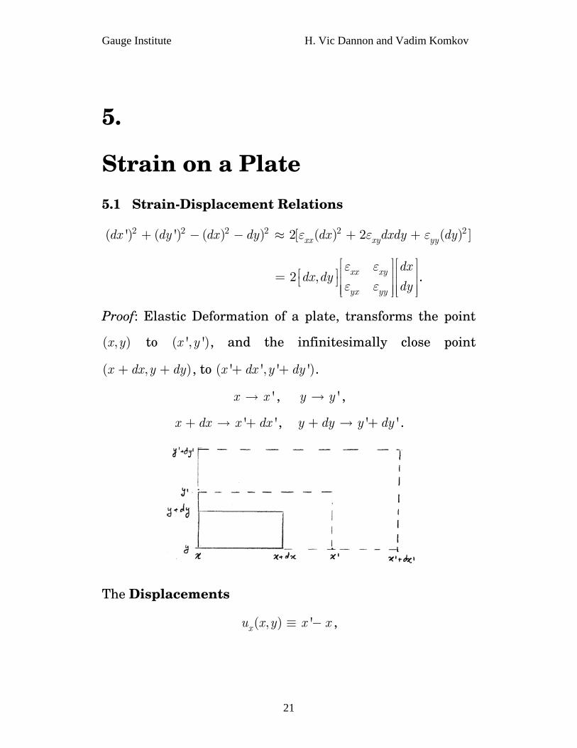
Proof: Elastic Deformation of a plate, transforms the point
to ( ' , and the infinitesimally close point
, to ( ' .
( , )x y , ')x y
( ,x dx y dy+ + ) ', ' ')x dx y dy+ +
'x x→ , , 'y y→
' 'x dx x dx+ → + , . ' 'y dy y dy+ → +
The Displacements
( , ) 'xu x y x x≡ − ,
21

Gauge Institute H. Vic Dannon and Vadim Komkov
( , ) 'yu x y y y≡ −
satisfy 'xdu dx dx= − , 'ydu dy dy= − .
Therefore,
2 2 2 2 2 2 2( ') ( ') [( ) ( ) ] ( ) ( ) ( ) ( )x ydx dy dx dy dx du dx dy du dy+ − + = + − + + − 2
)y
,
⎤⎥⎥⎥⎦
2 22 2 ( ) (x y xdxdu dydu du du= + + +
Keeping first order in , and in , xdu ydu
2 2x ydxdu dydu≈ +
{ }, , , ,2 [ ] [ ]x x x y y x y ydx u dx u dy dy u dx u dy= + + + .
, , ,
2 2
2[ ( ) ( ) ( ) ]
xx yyxy yx
x x x y y x y ydx u dx dx u u dy dy u dy
ε εε ε=
= + + +
. 2 , xx xy
yx yy
dxdx dy
dy
ε εε ε
⎡ ⎤ ⎡⎢ ⎥ ⎢⎡ ⎤= ⎣ ⎦ ⎢ ⎥ ⎢⎢ ⎥ ⎢⎣ ⎦ ⎣
5.2 The Axial Strains on a Plate are
,xx x xuε ≡ = elongation per unit length inx direction,
,yy y yuε ≡ = elongation per unit length in y direction.
5.3 Shear Strains on a Plate are
1, ,2
( )xy yx x y y xu uε ε= ≡ + .
22
Gauge Institute H. Vic Dannon and Vadim Komkov
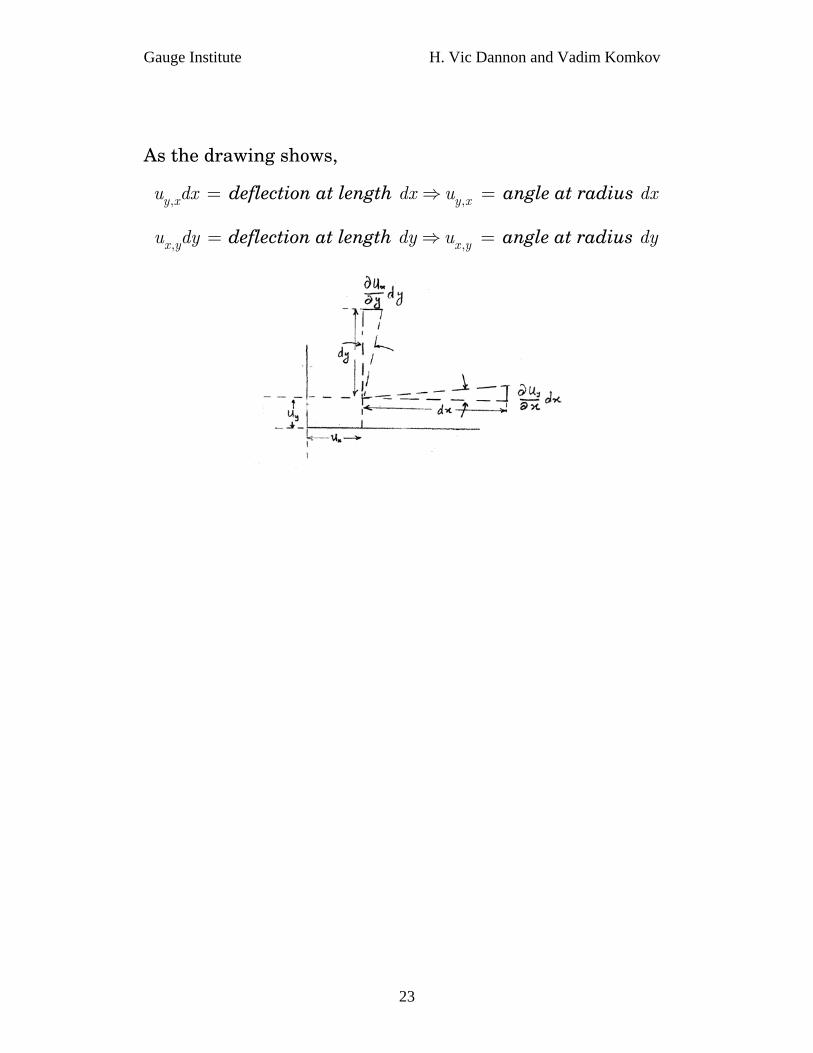
As the drawing shows,
,y xu dx = deflection at length dx angle at radius dx ⇒ ,y xu =
,x yu dy = deflection at length dy angle at radius dy ⇒ ,x yu =
23
Gauge Institute H. Vic Dannon and Vadim Komkov
6.
Stress on a Plate
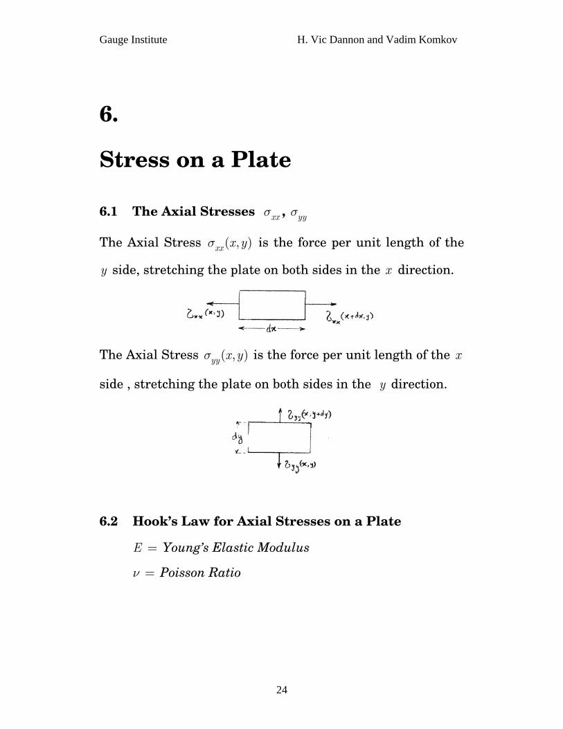
6.1 The Axial Stresses , xxσ yyσ
The Axial Stress is the force per unit length of the
side, stretching the plate on both sides in the x direction.
( , )xx x yσ
y
The Axial Stress is the force per unit length of the x
side , stretching the plate on both sides in the y direction.
( , )yy x yσ
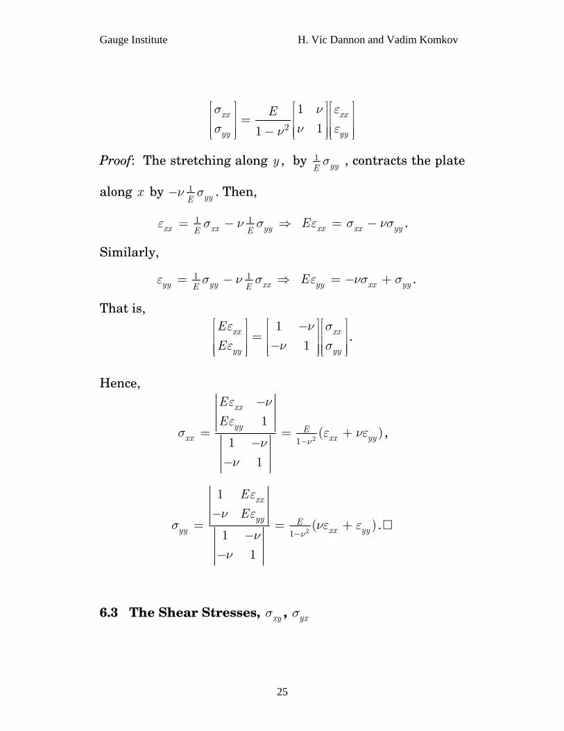
6.2 Hook’s Law for Axial Stresses on a Plate
Young’s Elastic Modulus E =
Poisson Ratio ν =
24
Gauge Institute H. Vic Dannon and Vadim Komkov
2
1
11xx xx
yy yy
Eσ νσ νν
⎡ ⎤ ⎡ ⎤ ⎡⎢ ⎥ ⎢ ⎥ ⎢=⎢ ⎥ ⎢ ⎥ ⎢−⎢ ⎥ ⎢ ⎥ ⎢⎣ ⎦ ⎣ ⎦ ⎣
εε
⎤⎥⎥⎥⎦
Proof: The stretching along y , by 1yyE
σ , contracts the plate
along x by 1yyE
ν σ− . Then,
1 1xx xx yyE Eε σ ν σ= − ⇒ E . xx xx yyε σ νσ= −
Similarly,
1 1yy yy xxE Eε σ ν σ= − ⇒ E . yy xx yyε νσ σ= − +
σσ
⎤⎥⎥⎥⎦
That is, 1
1xx xx
yy yy
E
E
ε νε ν
⎡ ⎤ ⎡ ⎤ ⎡−⎢ ⎥ ⎢ ⎥ ⎢=⎢ ⎥ ⎢ ⎥ ⎢−⎢ ⎥ ⎢ ⎥ ⎢⎣ ⎦ ⎣ ⎦ ⎣.
Hence,
21
1( )
1
1
xx
yy Exx xx yy
E
E
ν
ε νε
σ εν
ν
−
−
= = +−
−
νε ,
21
1
( )1
1
xx
yy Eyy xx yy
E
E
ν
εν ε
σ νε + εν
ν
−
−= =
−−
.
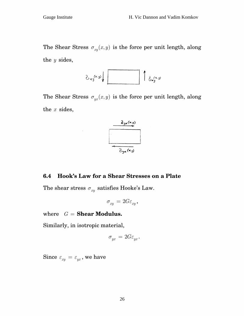
6.3 The Shear Stresses, , xyσ yxσ
25
Gauge Institute H. Vic Dannon and Vadim Komkov
The Shear Stress is the force per unit length, along
the y sides,
( , )xy x yσ
The Shear Stress is the force per unit length, along
the sides,
( , )yx x yσ
x
6.4 Hook’s Law for a Shear Stresses on a Plate
The shear stress satisfies Hooke’s Law. xyσ
2xy xyGσ ε= ,
where G Shear Modulus. =
Similarly, in isotropic material,
. 2yx yxGσ ε=
Since , we have xy yxε ε=
26

Gauge Institute H. Vic Dannon and Vadim Komkov
6.5 . xy yxσ σ=
6.6 Hook’s Law for a Plate
Young’s Elastic Modulus E =
Poisson Ratio ν =
G Shear Modulus=21
Eg
ν=
−
2
1 0
1 01
0 0 2
xx xx
yy yy
xy xy
E
g
σ νσ ν
νσ ε
⎡ ⎤ ⎡ ⎤ ⎡⎢ ⎥ ⎢ ⎥ ⎢⎢ ⎥ ⎢ ⎥ ⎢=⎢ ⎥ ⎢ ⎥ ⎢−⎢ ⎥ ⎢ ⎥ ⎢⎢ ⎥ ⎢ ⎥ ⎢⎣ ⎦ ⎣ ⎦ ⎣
εε
⎤⎥⎥⎥⎥⎥⎦
6.7 21E
Gν
=+
21xy xy xyE
Gσ εν
= =+
ε
Proof: By 6.2
2
1
11xx xx
yy yy
Eσ νσ νν
⎡ ⎤ ⎡ ⎤ ⎡⎢ ⎥ ⎢ ⎥ ⎢=⎢ ⎥ ⎢ ⎥ ⎢−⎢ ⎥ ⎢ ⎥ ⎢⎣ ⎦ ⎣ ⎦ ⎣
εε
⎤⎥⎥⎥⎦.
The matrix 1
1
νν
⎡ ⎤⎢ ⎥⎢ ⎥⎢ ⎥⎣ ⎦
27
Gauge Institute H. Vic Dannon and Vadim Komkov
has the eigen values 1 , and 1 , and can be rotated so
that
ν− ν+
' ' 11
' ' 121
01 0
0 1 01xx xx xx
yy yy yy
EE ν
ν
σ ν ενσ εν
+
−
⎡ ⎤ ⎡ ⎤ ⎡ ⎤'
'
ε
ε
⎡ ⎤⎡ ⎤−⎢ ⎥ ⎢ ⎥ ⎢ ⎥⎢ ⎥⎢ ⎥= =⎢ ⎥ ⎢ ⎥ ⎢ ⎥⎢ ⎥⎢ ⎥+− ⎢ ⎥⎢ ⎥ ⎢ ⎥ ⎢ ⎥⎢ ⎥⎣ ⎦ ⎣ ⎦⎣ ⎦ ⎣ ⎦ ⎣ ⎦,
That rotation diagonalizes also the matrix
1 0
1 0
0 0 2g
νν
⎡ ⎤⎢ ⎥⎢ ⎥⎢ ⎥⎢ ⎥⎢ ⎥⎣ ⎦
.
The equation for its eigen values yields
2gλ = ; ; . 1λ ν= + 1λ ν= −
For , 1λ ν= −
2 1g ν= − ,
22 (1 )
11
E EG ν
νν= − =
+−,
1xy xyE
σ εν
=+
.
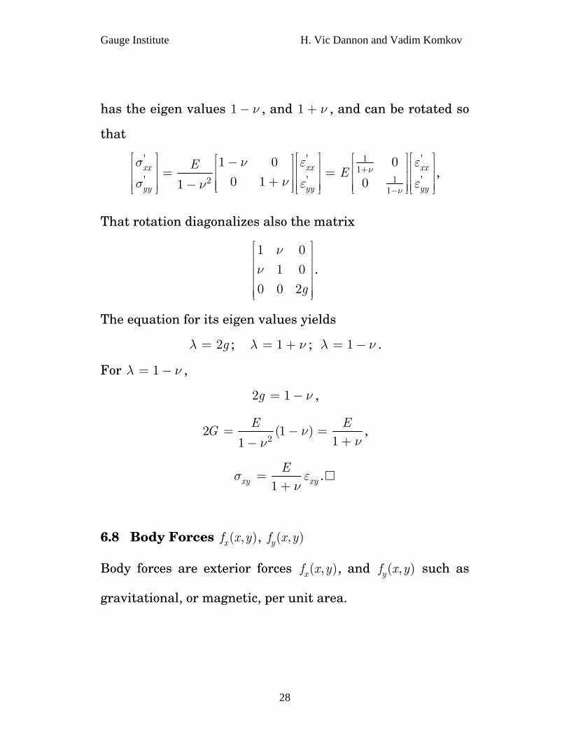
6.8 Body Forces ( , )xf x y , ( , )yf x y
Body forces are exterior forces ( , )xf x y , and ( , )yf x y such as
gravitational, or magnetic, per unit area.
28
Gauge Institute H. Vic Dannon and Vadim Komkov
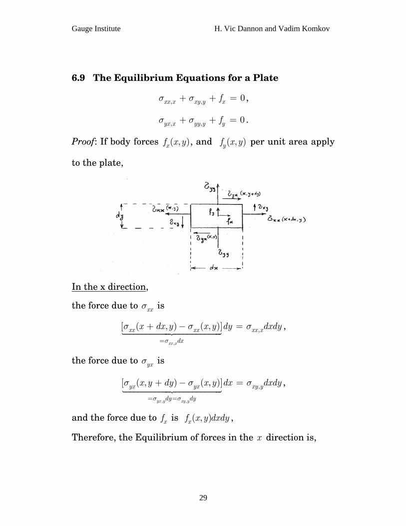
6.9 The Equilibrium Equations for a Plate
, , 0xx x xy y xfσ σ+ + = ,
, , 0yx x yy y yfσ σ+ + = .
Proof: If body forces ( , )xf x y , and ( , )yf x y per unit area apply
to the plate,
In the x direction,
the force due to is xxσ
,
,[ ( , ) ( , )]
xx x
xx xx xx x
dx
x dx y x y dy dxdy
σ
σ σ σ=
+ − = ,
the force due to is yxσ
, ,
,[ ( , ) ( , )]
yx y xy y
yx yx xy y
dy dy
x y dy x y dx dxdy
σ σ
σ σ σ
= =
+ − = ,
and the force due to xf is ( , )xf x y dxdy ,
Therefore, the Equilibrium of forces in the x direction is,
29
Gauge Institute H. Vic Dannon and Vadim Komkov
, , 0xx x xy y xfσ σ+ + = .
Similarly, the Equilibrium of forces in the y direction is,
, , 0yy y yx x yfσ σ+ + = .
30

Gauge Institute H. Vic Dannon and Vadim Komkov
7.
Strain Energy of a Plate 7.1 Infinitesimal Strain Energy per unit area
2xx xx xy xy yy yyd d d dμ σ ε σ ε σ ε= + +
. (summation over ; ) ij ijdσ ε= 1,2i = 1,2j =
xxxx
μσ
ε∂
=∂
; 2 xyxy
μσ
ε∂
=∂
; yyyy
μσ
ε∂
=∂
Proof: In the x direction,
The infinitesimal work done by , along is xxdyσ xdu
( , ) ( , )( ) ( ) ( )xx x xx x x xx xx dx y x ydydu dydu du dxdyσ σ σ
+− = ∂
, ,
[ ( ) ]
xx x x x
x xx x xx x x
du
du du dxdy
σ
σ σ= ∂ + ∂
The infinitesimal work done by , along is yxdxσ xdu
31

Gauge Institute H. Vic Dannon and Vadim Komkov
( , ) ( , )( ) ( ) ( )yx x yx x y yx xx y dy x ydxdu dxdu du dydxσ σ σ
+− = ∂
,,
[ ( ) ]
x yxy y
y yx x yx y x
du
du du dxdy
σ
σ σ= ∂ + ∂
The infinitesimal work by xf dxdy is ( , )x xf x y dxdydu
In the y direction,
The infinitesimal work done by , along is yydxσ ydu
( , ) ( , )( ) ( ) ( )yy y yy y y yy yx y dy x ydxdu dxdu du dxdyσ σ σ
+− = ∂
,,
[ ( ) ]
y yyy y
y yy y yy y y
du
du du dxdy
σ
σ σ= ∂ + ∂
The infinitesimal work done by , along is xydyσ ydu
( , ) ( , )( ) ( ) ( )xy y xy y x xy yx dx y x ydydu dydu du dxdyσ σ σ
+− = ∂
,,
[ ( ) ]
y xxy x
x yx y yx x y
du
du du dxdy
σ
σ σ= ∂ + ∂
The infinitesimal work by yf is ( , )y yf x y dxdydu
32
Gauge Institute H. Vic Dannon and Vadim Komkov
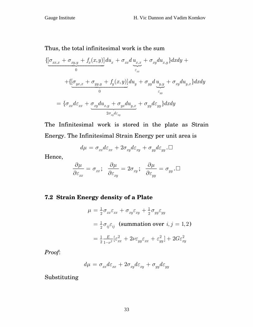
Thus, the total infinitesimal work is the sum
+ , , , ,
0
{[ ( , )] }
xx
xx x xy y x x xx x x xy x yf x y du d u du dxdy
ε
σ σ σ σ+ + + +
, , , ,
0
{[ ( , )] }
yy
yx x yy y y y yy y y xy y xf x y du d u du dxdy
ε
σ σ σ σ+ + + + +
, ,
2
{ }
xy xy
xx xx xy x y yx y x yy yy
d
d du du d d
σ ε
σ ε σ σ σ ε= + + + xdy
The Infinitesimal work is stored in the plate as Strain
Energy. The Infinitesimal Strain Energy per unit area is
2xx xx xy xy yy yyd d d dμ σ ε σ ε σ ε= + + .
Hence,
xxxx
μσ
ε∂
=∂
; 2 xyxy
μσ
ε∂
=∂
; yyyy
μσ
ε∂
=∂
.
7.2 Strain Energy density of a Plate
1 12 2xx xx xy xy yy yyμ σ ε σ ε σ ε= + +
12 ij ijσ ε= (summation over ) , 1,i j = 2
2
2 212 1
[ 2 ] 2Exx yy xx yy xyG
νε νε ε ε ε
−= + + + 2
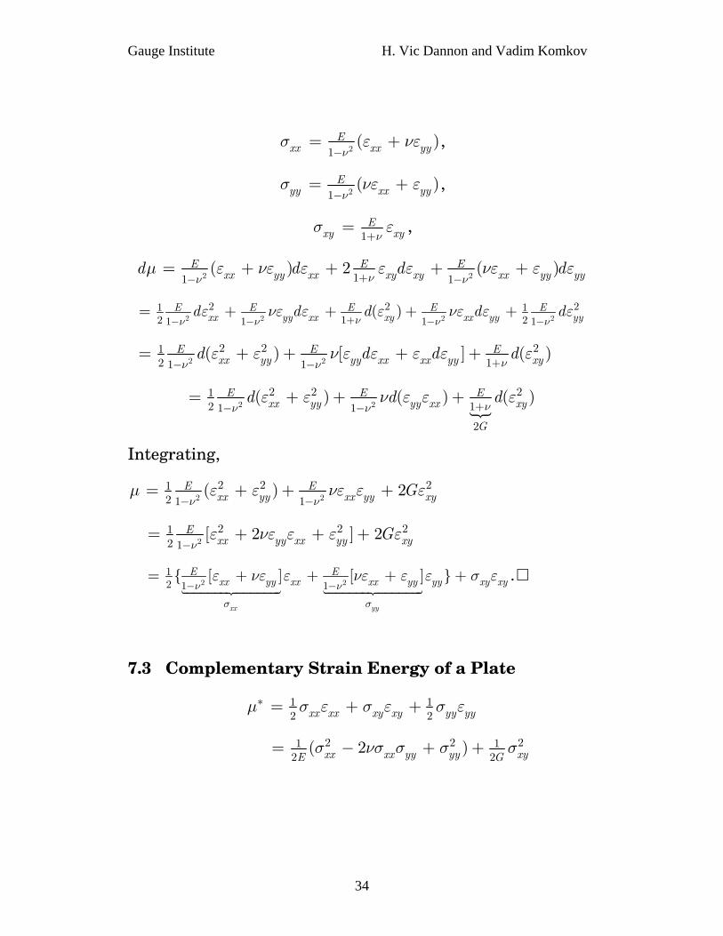
Proof:
2xx xx xy xy yy yyd d d dμ σ ε σ ε σ ε= + +
Substituting
33
Gauge Institute H. Vic Dannon and Vadim Komkov
21( )E
xx xx yyνσ ε
−= + νε ,
21( )E
yy xx yyνσ νε
−= + ε ,
1E
xy xyνσ ε
+= ,
2 211 1( ) 2 (E E Exx yy xx xy xy xx yy yyd d d
νν νμ ε νε ε ε ε νε ε
+− −= + + + + )dε
2 2 2 22 21 1
2 11 1 1 1( )E E E E E
xx yy xx xy xx yy yyd d d dνν ν ν ν
ε νε ε ε νε ε+− − − −
= + + + + 22
dε
2 2
2 2 212 11 1
( ) [ ] (E Exx yy yy xx xx yy xyd d d
νν νε ε ν ε ε ε ε ε
+− −= + + + + )E d
2 22 2 21
2 11 1
2
( ) ( ) (E Exx yy yy xx xy
G
d dνν ν
ε ε ν ε ε ε+− −
= + + + )E d
Integrating,
2 22 21
2 1 1( ) 2E Exx yy xx yy xyG
ν νμ ε ε νε ε
− −= + + + 2ε
2
2 212 1
[ 2 ] 2Exx yy xx yy xyG
νε νε ε ε ε
−= + + + 2
2 2
12 1 1{ [ ] [ ] }
xx yy
E Exx yy xx xx yy yy xy xyν ν
σ σ
ε νε ε νε ε ε σ ε− −
= + + + + .
7.3 Complementary Strain Energy of a Plate
1 12 2xx xx xy xy yy yyμ σ ε σ ε σ∗ = + + ε
2 21 12 2
( 2 )xx xx yy yy xyE Gσ νσ σ σ σ= − + + 2
34
Gauge Institute H. Vic Dannon and Vadim Komkov
xxxx
με
σ
∗∂=
∂; 2 xy
xy
με
σ
∗∂=
∂; yy
yy
με
σ
∗∂=
∂
Proof: The complementary strain energy density is the
strain energy density expressed in terms of the stresses.
Substituting 1 1
xx xx yyE Eε σ ν= − σ
1 1yy yy xxE Eε σ ν= − σ
12xy xyG
ε σ=
into μ ,
1 12 2xx xx xy xy yy yyμ σ ε σ ε σ ε= + +
1 1 12 2 2
( ) (xx xx yy xy xy yy xx yyE G Eσ σ νσ σ σ σ νσ σ= − + + − + )
2 21 12 2
( 2 )xx xx yy yy xyE Gσ νσ σ σ σ= − + + 2
Although equals , it is denoted by μ to specify its
dependence on the stress.
μ∗ μ ∗
1 1xx yy xxE E
xx
μσ ν σ ε
σ
∗∂= − =
∂.
1 1yy xx yyE E
yy
μσ ν σ ε
σ
∗∂= − =
∂
1 2xy xyGxy
μσ ε
σ
∗∂= =
∂.
35
Gauge Institute H. Vic Dannon and Vadim Komkov
8.
Variational Principles on a
Plate
8.1 Euler’s Variational Equations
The deflections , and that minimize or maximize xu yu
the plate’s energy per unit area,
( , , , , , , )x y xx xy yyF F x y u u ε ε ε=
satisfy Euler’s Variational Equation
( , , , , , , ) 0x y xx xy yyF x y u uδ ε ε ε = ,
which is,
1 12 2
0x y x x y yx xx xy y xy yy
F F F F F Fu u
u uδ δ
ε ε ε ε
⎛ ⎞ ⎛∂ ∂ ∂ ∂ ∂ ∂⎟ ⎟⎜ ⎜⎟ ⎟⎜ ⎜− ∂ − ∂ + − ∂ − ∂ =⎟ ⎟⎜ ⎜⎟ ⎟⎟ ⎟⎜ ⎜∂ ∂ ∂ ∂ ∂ ∂⎝ ⎠ ⎝
⎞
⎠.
or, 12
0x yx xx xy
F F Fu ε ε
∂ ∂ ∂− ∂ − ∂ =
∂ ∂ ∂,
12
0x yy xy yy
F F Fu ε ε
∂ ∂ ∂− ∂ − ∂ =
∂ ∂ ∂.
Proof: The Plate’s infinitesimal energy is
36
Gauge Institute H. Vic Dannon and Vadim Komkov
1 12 2
1 12 2
( , , , , , , )
x dx y dy
x dx y dy
F u u d d
ξ η
ξ η ξξ ξη ηηξ η
ξ η ε ε ε ξ η= + = +
= − = −∫ ∫ .
The deflections , and that minimizes or maximize the
plate’s energy, satisfy Euler’s Variational Equation
xu yu
( , , , , , , ) 0x y xx xy yyF x y u uδ ε ε ε = .
That is,
1 12 2
0
x x y yy x x y
x xx xy y yyx xx xy y yyu uu u
F F F F Fu u
u uδ δδ δ
δ δε δε δ δεε ε ε
∂ ∂∂ + ∂
∂ ∂ ∂ ∂ ∂+ + + +
∂ ∂ ∂ ∂ ∂=
1 12 2
0x x x y x y x y y yx xx xy y xy yy
F F F F F Fu u u u u u
u uδ δ δ δ δ δ
ε ε ε ε∂ ∂ ∂ ∂ ∂ ∂
+ ∂ + ∂ + + ∂ + ∂ =∂ ∂ ∂ ∂ ∂ ∂
Integration by parts, where , and vanish on the
boundary, [Dan3] leads to the variational equation
xuδ yuδ
1 12 2
0x y x x y yx xx xy y xy yy
F F F F F Fu u
u uδ δ
ε ε ε ε
⎛ ⎞ ⎛∂ ∂ ∂ ∂ ∂ ∂⎟ ⎟⎜ ⎜⎟ ⎟⎜ ⎜− ∂ − ∂ + − ∂ − ∂ =⎟ ⎟⎜ ⎜⎟ ⎟⎟ ⎟⎜ ⎜∂ ∂ ∂ ∂ ∂ ∂⎝ ⎠ ⎝
⎞
⎠.
Since the variations , and are independent, the
deflections , and that minimizes or maximize the
plates’s energy satisfy Euler’s Variational Equations
xuδ yuδ
xu yu
37
Gauge Institute H. Vic Dannon and Vadim Komkov
12
0x yx xx xy
F F Fu ε ε∂ ∂ ∂
− ∂ − ∂ =∂ ∂ ∂
12
0x yy xy yy
F F Fu ε ε
∂ ∂ ∂− ∂ − ∂ =
∂ ∂ ∂
8.2 If the body forces originate from a Potential per ( , )x yu uυ
unit area, so that
xx
fuυ∂
− =∂
yy
fuυ∂
− =∂
Then, Euler’s Equations are the Equilibrium Equations
, , 0xx x xy y xfσ σ+ + =
, , 0yx x yy y yfσ σ+ + = .
Proof: The Energy per unit area is
( , , , , , , )x y xx xy yyF x y u u ε ε ε μ υ= +
1 12 2xx xx xy xy yy yyσ ε σ ε σ ε υ= + + + .
The Euler’s Variational Equations are
38
Gauge Institute H. Vic Dannon and Vadim Komkov
12
2
0
x xx xy
x yx xx xy
f
F F Fu
σ σ
ε ε−
∂ ∂ ∂− ∂ − ∂ =
∂ ∂ ∂
12
0
y yx yy
x yy xy yy
f
F F Fu
σ σ
ε ε
−
∂ ∂ ∂− ∂ − ∂ =
∂ ∂ ∂
That is, Euler’s Equations are the equilibrium Equations
0x x xx y xyf σ σ+ ∂ + ∂ = ,
0y x yx y yyf σ σ+ ∂ + ∂ = .
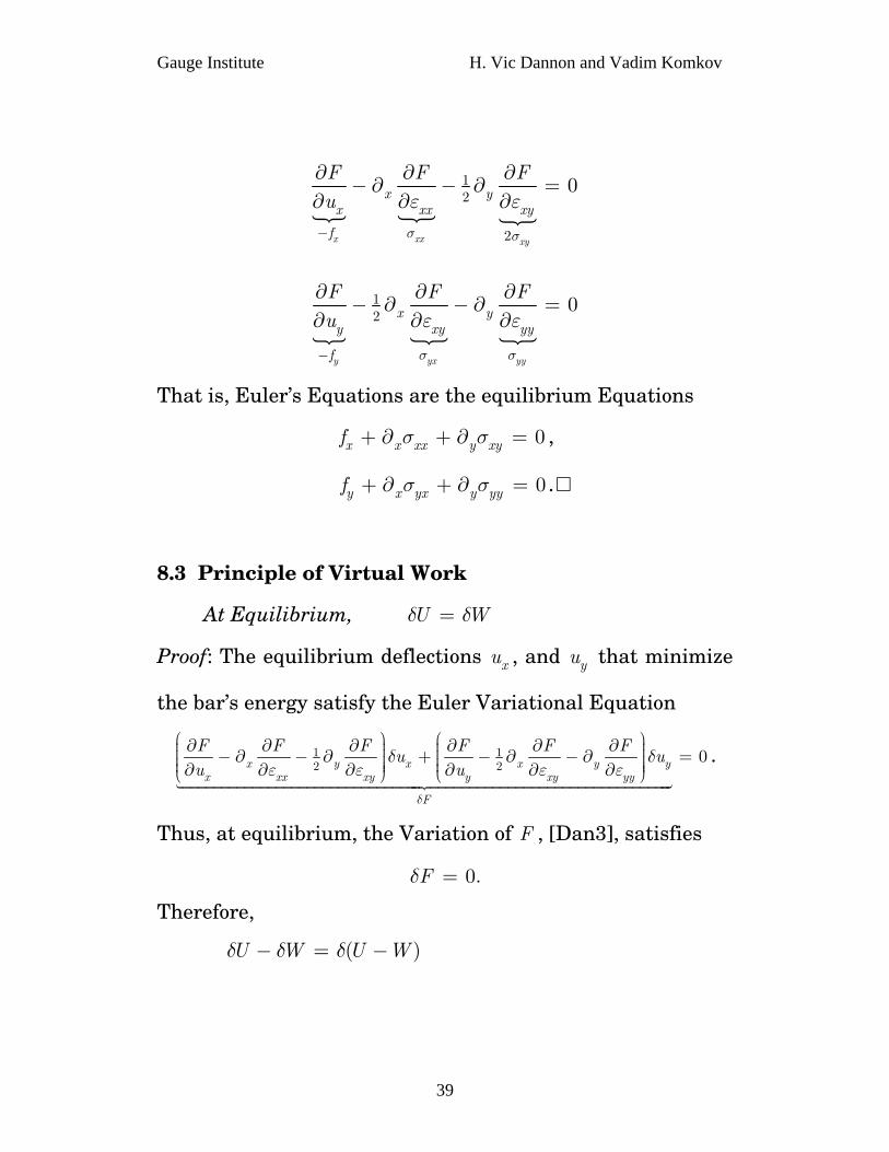
8.3 Principle of Virtual Work
At Equilibrium, U Wδ δ=
Proof: The equilibrium deflections , and that minimize
the bar’s energy satisfy the Euler Variational Equation
xu yu
1 12 2
0x y x x y yx xx xy y xy yy
F
F F F F F Fu u
u u
δ
δ δε ε ε ε
⎛ ⎞ ⎛∂ ∂ ∂ ∂ ∂ ∂⎟ ⎟⎜ ⎜⎟ ⎟⎜ ⎜− ∂ − ∂ + − ∂ − ∂ =⎟ ⎟⎜ ⎜⎟ ⎟⎟ ⎟⎜ ⎜∂ ∂ ∂ ∂ ∂ ∂⎝ ⎠ ⎝
⎞
⎠.
Thus, at equilibrium, the Variation of F , [Dan3], satisfies
0.Fδ =
Therefore,
( )U W U Wδ δ δ− = −
39
Gauge Institute H. Vic Dannon and Vadim Komkov
0 0
( , , , , , , )yx
y lx l
x y xx xy yyx y
F x y u u dxdyδ ε ε==
= =
= ∫ ∫ ε
0 0
( , , , , , , ) 0yx
y lx l
x y xx xy yyx y
F x y u u dxdyδ ε ε ε==
= =
= =∫ ∫
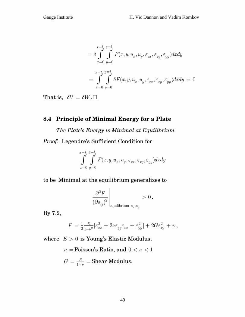
That is, . U Wδ δ=
8.4 Principle of Minimal Energy for a Plate
The Plate’s Energy is Minimal at Equilibrium
Proof: Legendre’s Sufficient Condition for
0 0
( , , , , , , )yx
y lx l
x y xx xy yyx y
F x y u u dxdyε ε ε==
= =∫ ∫
to be Minimal at the equilibrium generalizes to
2
2equilibrium ;
0( )
x yij u u
F
ε
∂>
∂.
By 7.2,
22 21
2 1[ 2 ] 2Exx yy xx yy xyF G
νε νε ε ε ε
−= + + + 2 υ+ ,
where is Young’s Elastic Modulus, 0E >
ν Poisson’s Ratio, and = 0 1ν< <
1EGν+
= =Shear Modulus.
40
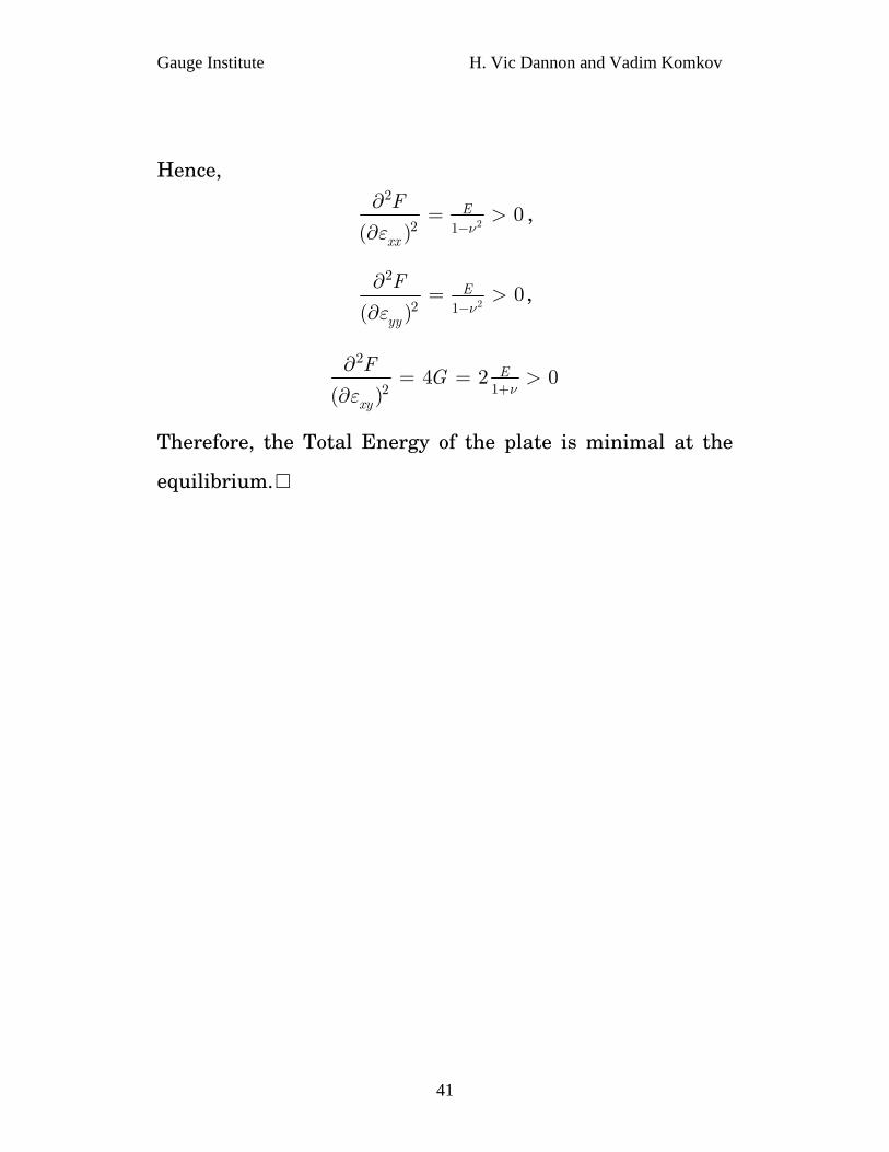
Gauge Institute H. Vic Dannon and Vadim Komkov
Hence,
2
2
2 10
( )E
xx
Fνε −
∂= >
∂,
2
2
2 10
( )E
yy
Fνε −
∂= >
∂,
2
124 2
( )E
xy
FG
νε +
∂= = >
∂0
Therefore, the Total Energy of the plate is minimal at the
equilibrium.
41
Gauge Institute H. Vic Dannon and Vadim Komkov
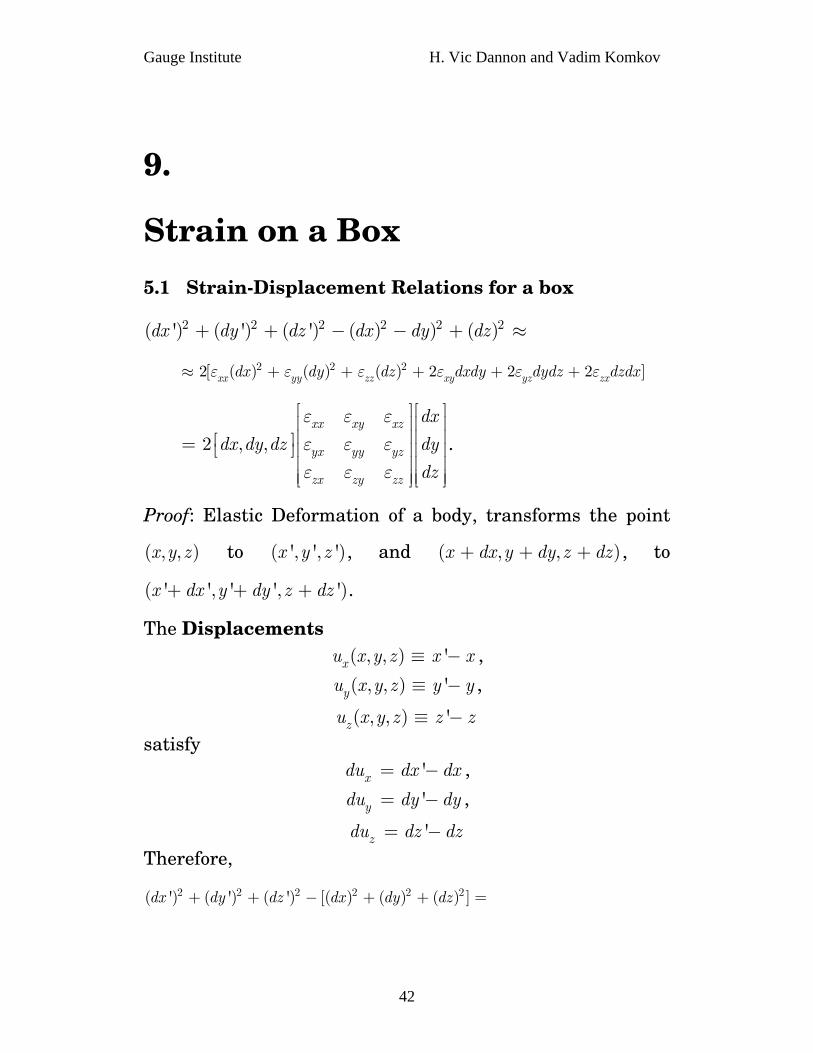
9.
Strain on a Box
5.1 Strain-Displacement Relations for a box
2 2 2 2 2 2( ') ( ') ( ') ( ) ) ( )dx dy dz dx dy dz+ + − − + ≈
⎡ ⎤⎢ ⎥⎢ ⎥⎢ ⎥⎢ ⎥⎢ ⎥⎣ ⎦
)
=
2 2 22[ ( ) ( ) ( ) 2 2 2 ]xx yy zz xy yz zxdx dy dz dxdy dydz dzdxε ε ε ε ε ε≈ + + + + +
. 2 , ,xx xy xz
yx yy yz
zx zy zz
dx
dx dy dz dy
dz
ε ε εε ε εε ε ε
⎡ ⎤⎢ ⎥⎢ ⎥⎡ ⎤= ⎢ ⎥⎣ ⎦⎢ ⎥⎢ ⎥⎣ ⎦
Proof: Elastic Deformation of a body, transforms the point
to ( ' , and ( , , to
.
( , , )x y z , ', ')x y z ,x dx y dy z dz+ + +
( ' ', ' ', ')x dx y dy z dz+ + +
The Displacements ( , , ) 'xu x y z x x≡ − , ( , , ) 'yu x y z y y≡ − ,
( , , ) 'zu x y z z z≡ − satisfy
'xdu dx dx= − , 'ydu dy dy= − ,
'zdu dz dz= − Therefore,
2 2 2 2 2 2( ') ( ') ( ') [( ) ( ) ( ) ]dx dy dz dx dy dz+ + − + +
42

Gauge Institute H. Vic Dannon and Vadim Komkov
2 22 2 2 ( ) ( ) (x y z x ydxdu dydu dzdu du du du= + + + + + 2)z
z
+
+
}
,
Keeping first order in , , and xdu ydu zdu
2 2 2x ydxdu dydu dzdu≈ + +
, , ,2{ [ ]x x x y x zdx u dx u dy u dz= + +
, , ,[ ]y x y y y zdy u dx u dy u dz+ + +
. , , ,[ ]z x z y z zdz u dx u dy u dz+ + +
, ,2[ ( ) ( ) ( ) ]
xx yy zz
x x y y z zdx u dx dy u dy dz u dz
ε ε ε
= + +
, , , , , ,
2 2 2 2 2 2
2[ ( ) ( ) ( ) ]
xy yx yz zy zx xz
x y y x y z z y z x x zdx u u dy dy u u dz dz u u dx
ε ε ε ε ε ε= = =
+ + + + + +
2 , ,xx xy xz
yx yy yz
zx zy zz
dx
dx dy dz dy
dz
ε ε εε ε εε ε ε
⎡ ⎤ ⎡ ⎤⎢ ⎥ ⎢ ⎥⎢ ⎥ ⎢ ⎥⎡ ⎤= ⎢ ⎥ ⎢ ⎥⎣ ⎦⎢ ⎥ ⎢ ⎥⎢ ⎥ ⎢ ⎥⎣ ⎦ ⎣ ⎦
.
5.2 The Axial Strains on a Box are
, ( , , )xx x xu x y zε ≡ =
=
=
elongation per unit length inx direction,
elongation per unit length in y direction, , ( , , )yy y yu x y zε ≡
elongation per unit length in y direction. , ( , , )zz z zu x y zε ≡
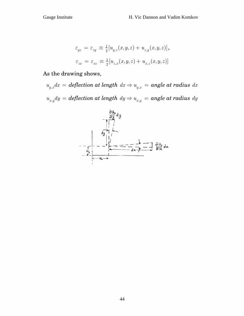
5.3 Shear Strains on the faces of a Box are
1, ,2
[ ( , , ) ( , ,xy yx x y y xu x y z u x y zε ε= ≡ + )],
43
Gauge Institute H. Vic Dannon and Vadim Komkov
1, ,2
[ ( , , ) ( , , )yz zy y z z yu x y z u x y zε ε= ≡ + ],
1, ,2
[ ( , , ) ( , , )zx xz z x x zu x y z u x y zε ε= ≡ + ]
As the drawing shows,
,y xu dx = deflection at length dx angle at radius dx ⇒ ,y xu =
,x yu dy = deflection at length dy angle at radius dy ⇒ ,x yu =
44
Gauge Institute H. Vic Dannon and Vadim Komkov
10.
Stress on a Box
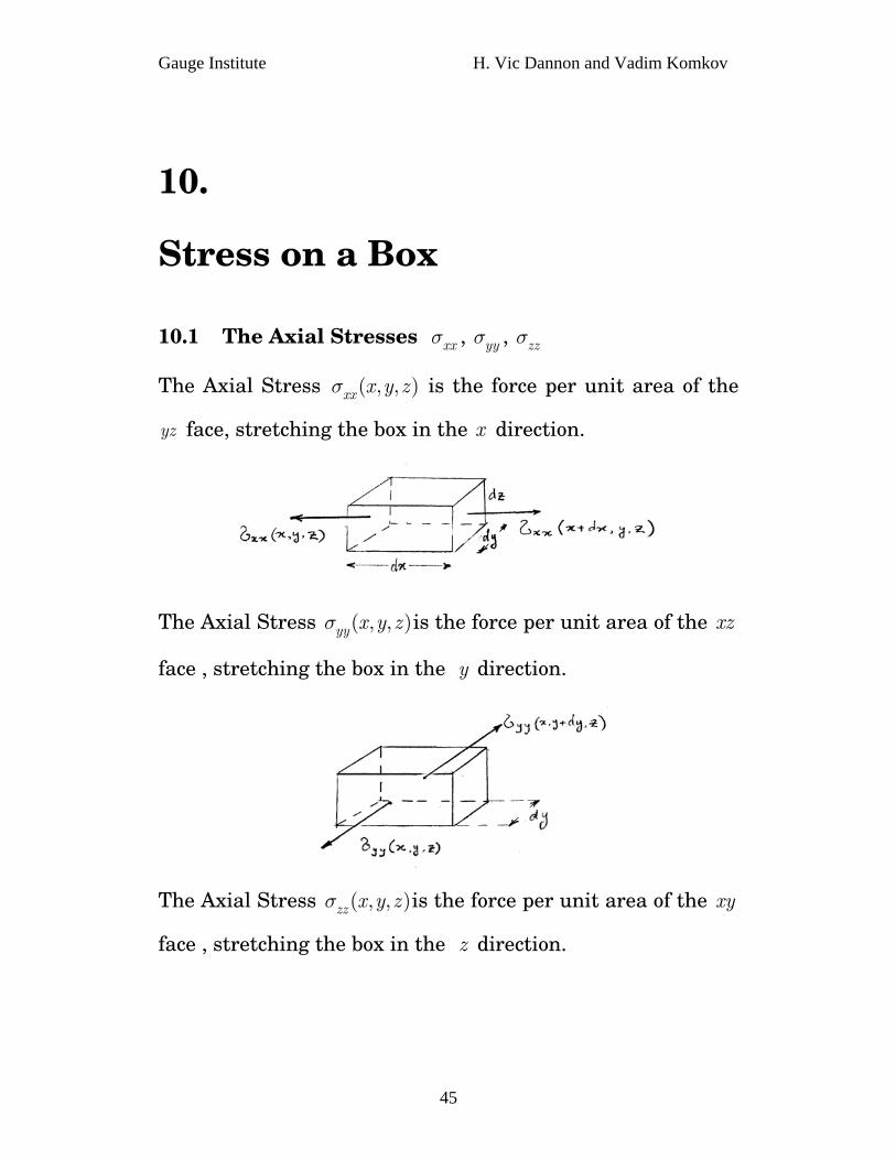
10.1 The Axial Stresses , , xxσ yyσ zzσ
The Axial Stress is the force per unit area of the
face, stretching the box in the x direction.
( , , )xx x y zσ
yz
The Axial Stress is the force per unit area of the xz
face , stretching the box in the y direction.
( , , )yy x y zσ
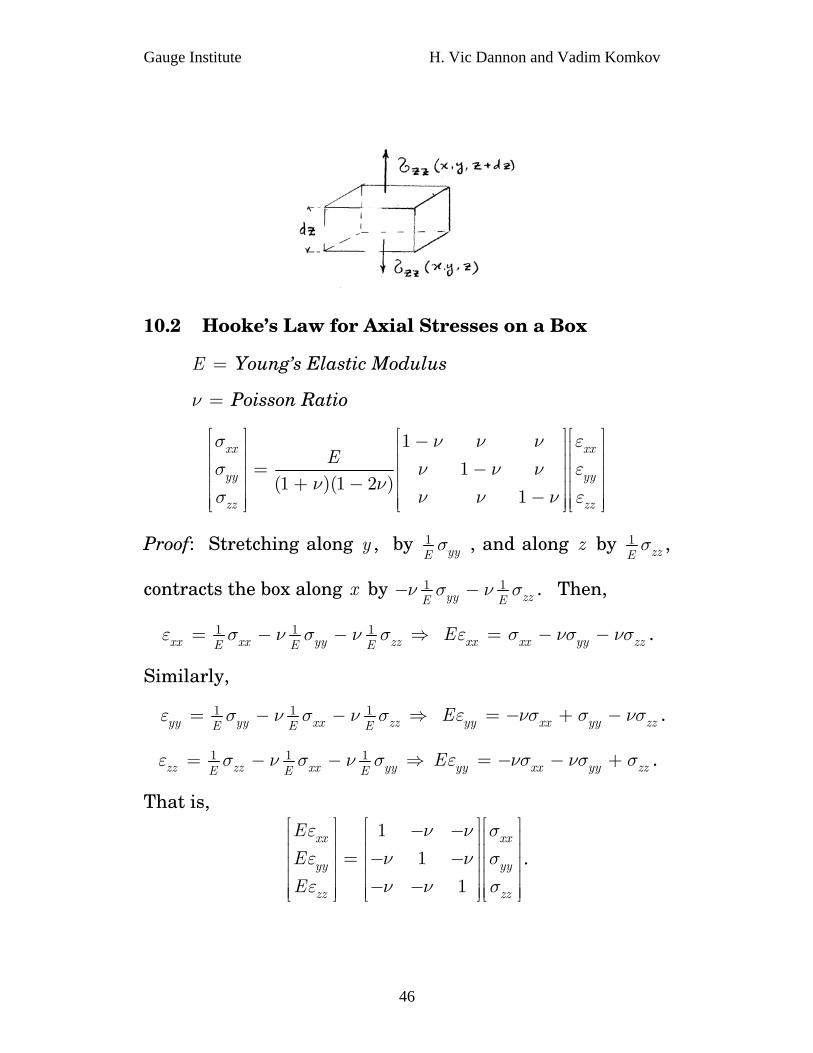
The Axial Stress is the force per unit area of the xy
face , stretching the box in the z direction.
( , , )zz x y zσ
45
Gauge Institute H. Vic Dannon and Vadim Komkov
10.2 Hooke’s Law for Axial Stresses on a Box
Young’s Elastic Modulus E =
Poisson Ratio ν =
1
1(1 )(1 2 )
1
xx xx
yy yy
zz zz
Eσ ν νσ ν ν
ν νσ ν ν
⎡ ⎤ ⎡ ⎤ ⎡−⎢ ⎥ ⎢ ⎥ ⎢⎢ ⎥ ⎢ ⎥ ⎢= −⎢ ⎥ ⎢ ⎥ ⎢+ −⎢ ⎥ ⎢ ⎥ ⎢−⎢ ⎥ ⎢ ⎥ ⎢⎣ ⎦ ⎣ ⎦ ⎣
ν εν εν ε
⎤⎥⎥⎥⎥⎥⎦
Proof: Stretching along y , by 1yyE
σ , and along by z 1zzE
σ ,
contracts the box along x by 1 1yy zzE E
ν σ ν σ− − . Then,
1 1 1xx xx yy zzE E Eε σ ν σ ν σ= − − ⇒ . xx xx yy zzEε σ νσ νσ= − −
Similarly,
1 1 1yy yy xx zzE E Eε σ ν σ ν σ= − − ⇒ E . yy xx yy zzε νσ σ νσ= − + −
1 1 1zz zz xx yyE E Eε σ ν σ ν σ= − − ⇒ E . yy xx yy zzε νσ νσ σ= − − +
σσσ
⎤⎥⎥⎥⎥⎥⎦
That is, 1
1
1
xx xx
yy yy
zz zz
E
E
E
ε ν νε ν νε ν ν
⎡ ⎤ ⎡ ⎤ ⎡− −⎢ ⎥ ⎢ ⎥ ⎢⎢ ⎥ ⎢ ⎥ ⎢= − −⎢ ⎥ ⎢ ⎥ ⎢⎢ ⎥ ⎢ ⎥ ⎢− −⎢ ⎥ ⎢ ⎥ ⎢⎣ ⎦ ⎣ ⎦ ⎣
.
46
Gauge Institute H. Vic Dannon and Vadim Komkov
Since
2
1
1 (1 ) (1
1
ν νν ν νν ν
− −− − = + −
− −
2 )ν ,
(1 )(1 2 )
1
1[(1 ) ]
1
1
1
xx
yy
zz Exx xx yy zz
E
E
Eν ν
ε ν νε νε ν
σ νν ν
ν νν ν
+ −
− −−
−= = − +
− −− −− −
ε νε νε+ ,
(1 )(1 2 )[ (1 )E
yy xx yy zzν νσ νε ν ε
+ −= + − ]νε+ ,
(1 )(1 2 )[ (1 )ν− ]E
zz xx yy zzν νσ νε νε ε
+ −= + + .
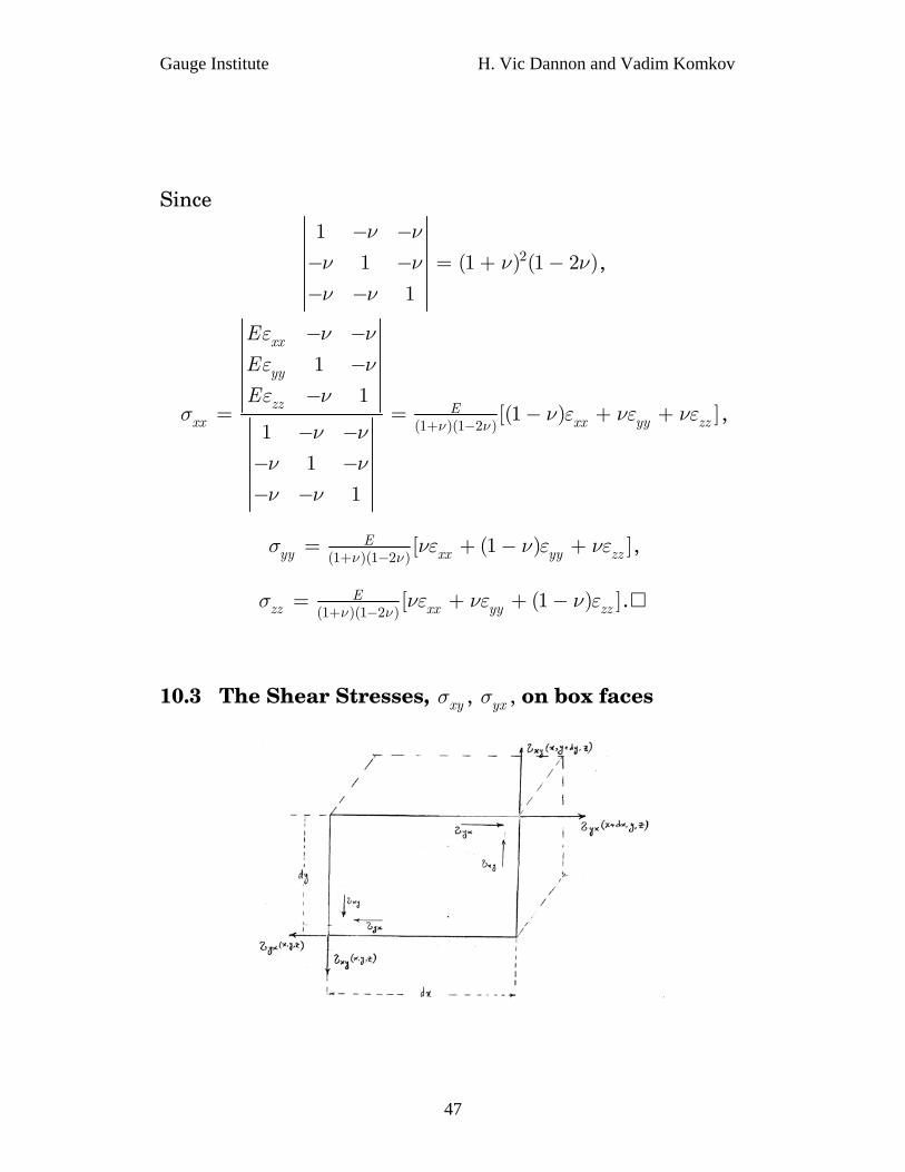
10.3 The Shear Stresses, , , on box faces xyσ yxσ
47
Gauge Institute H. Vic Dannon and Vadim Komkov
The Shear Stress is the force per unit area in the
plane, along y ,
( , , )xy x y zσ
xy
The Shear Stress is the force per unit area in yx
plane, along x ,
( , , )yx x y zσ
10.4 Hooke’s Law for a Shear Stresses on box faces
The shear stress satisfies Hooke’s Law. xyσ
2xy xyGσ ε= ,
2yz yzGσ ε= ,
2zx zxGσ ε= .
where G Shear Modulus. =
Similarly, in isotropic material,
2yx yxGσ ε= ,
2zy zyGσ ε= ,
2xz xzGσ ε= .
10.5 ; ; . xy yxσ σ= yz zyσ σ= xy yxσ σ=
Proof: Since , , . xy yxε ε= yz zyε ε= zx xzε ε=
48
Gauge Institute H. Vic Dannon and Vadim Komkov
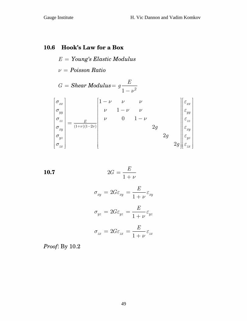
10.6 Hook’s Law for a Box
Young’s Elastic Modulus E =
Poisson Ratio ν =
G Shear Modulus=21
Eg
ν=
−
(1 )(1 2 )
1
1
0 1
2
2
2
xx xx
yy yy
zz zzE
xy xy
yz yz
zx zx
g
g
g
ν ν
σ ν ν νσ ν ν νσ ν νσ εσ εσ ε
+ −
⎡ ⎤ ⎡ ⎤ ⎡−⎢ ⎥ ⎢ ⎥ ⎢⎢ ⎥ ⎢ ⎥ ⎢−⎢ ⎥ ⎢ ⎥ ⎢⎢ ⎥ ⎢ ⎥ ⎢−⎢ ⎥ ⎢ ⎥ ⎢=⎢ ⎥ ⎢ ⎥ ⎢⎢ ⎥ ⎢ ⎥ ⎢⎢ ⎥ ⎢ ⎥ ⎢⎢ ⎥ ⎢ ⎥ ⎢⎢ ⎥ ⎢ ⎥ ⎢⎢ ⎥ ⎢ ⎥ ⎢⎣ ⎦ ⎣ ⎦ ⎣
εεε
⎤⎥⎥⎥⎥⎥⎥⎥⎥⎥⎥⎥⎦
10.7 21E
Gν
=+
21xy xy xyE
Gσ εν
= =+
ε
21yz yz yzE
Gσ εν
= =+
ε
21zx zx zxE
Gσ εν
= =+
ε
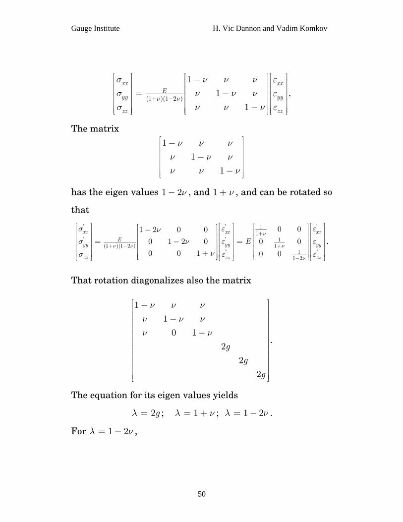
Proof: By 10.2
49
Gauge Institute H. Vic Dannon and Vadim Komkov
(1 )(1 2 )
1
1
1
xx xxE
yy yy
zz zz
ν ν
σ ν νσ ν νσ ν ν
+ −
⎡ ⎤ ⎡ ⎤ ⎡−⎢ ⎥ ⎢ ⎥ ⎢⎢ ⎥ ⎢ ⎥ ⎢= −⎢ ⎥ ⎢ ⎥ ⎢⎢ ⎥ ⎢ ⎥ ⎢−⎢ ⎥ ⎢ ⎥ ⎢⎣ ⎦ ⎣ ⎦ ⎣
ν εν εν ε
⎤⎥⎥⎥⎥⎥⎦
ν
.
The matrix 1
1
1
ν ν νν ν νν ν
⎡ ⎤−⎢ ⎥⎢ ⎥−⎢ ⎥⎢ ⎥−⎢ ⎥⎣ ⎦
has the eigen values 1 , and 1 , and can be rotated so
that
2ν− ν+
' ' 11
' ' 1(1 )(1 2 ) 1
' ' 11 2
0 01 2 0 0
0 1 2 0 0 0
0 0 1 0 0
xx xx xxE
yy yy yy
zz zz zz
Eν
ν ν ν
ν
σ ενσ ν ε
νσ ε
+
+ − +
−
⎡ ⎤ ⎡ ⎤ ⎡ ⎤'
'
'
ε
ε
ε
⎡ ⎤⎡ ⎤−⎢ ⎥ ⎢ ⎥ ⎢ ⎥⎢ ⎥⎢ ⎥⎢ ⎥ ⎢ ⎥ ⎢ ⎥⎢ ⎥⎢ ⎥= − =⎢ ⎥ ⎢ ⎥ ⎢ ⎥⎢ ⎥⎢ ⎥⎢ ⎥ ⎢ ⎥ ⎢ ⎥⎢ ⎥⎢ ⎥+⎢ ⎥ ⎢ ⎥ ⎢ ⎥⎢ ⎥⎢ ⎥⎣ ⎦ ⎣ ⎦⎣ ⎦ ⎣ ⎦ ⎣ ⎦
.
That rotation diagonalizes also the matrix
1
1
0 1
2
2
2
g
g
g
ν ν νν ν νν ν
⎡ ⎤−⎢ ⎥⎢ ⎥−⎢ ⎥⎢ ⎥−⎢ ⎥⎢ ⎥⎢ ⎥⎢ ⎥⎢ ⎥⎢ ⎥⎢ ⎥⎣ ⎦
.
The equation for its eigen values yields
2gλ = ; ; . 1λ ν= + 1 2λ ν= −
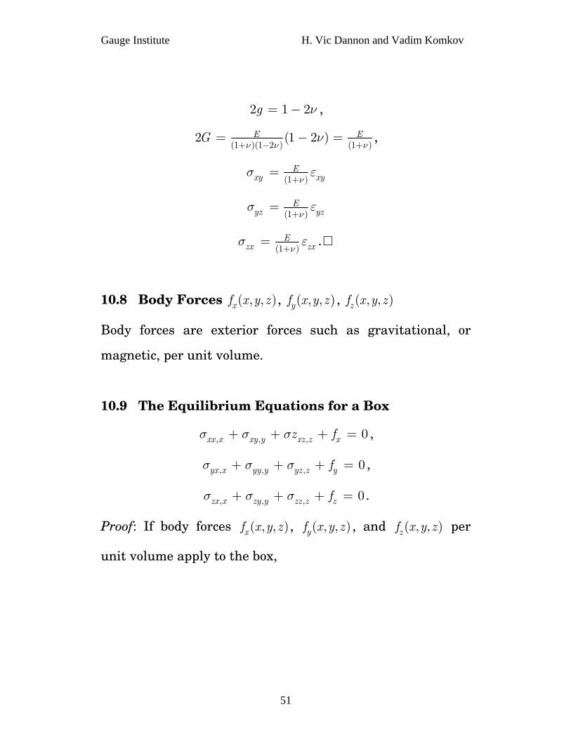
For , 1 2λ ν= −
50
Gauge Institute H. Vic Dannon and Vadim Komkov
2 1 2g ν= − ,
(1 )(1 2 ) (1 )2 (1 2 )E EG
ν νν
+ − += − =
ν,
(1 )E
xy xyνσ ε
+=
(1 )E
yz yzνσ ε
+=
(1 )E
zx zxνσ ε
+= .
10.8 Body Forces ( , , )xf x y z , ( , , )yf x y z , ( , , )zf x y z
Body forces are exterior forces such as gravitational, or
magnetic, per unit volume.
10.9 The Equilibrium Equations for a Box
, , , 0xx x xy y xz z xz fσ σ σ+ + + = ,
, , , 0yx x yy y yz z yfσ σ σ+ + + = ,
, , , 0zx x zy y zz z zfσ σ σ+ + + = .
Proof: If body forces ( , , )xf x y z , ( , , )yf x y z , and ( , , )zf x y z per
unit volume apply to the box,
51
Gauge Institute H. Vic Dannon and Vadim Komkov
In the x direction,
the force due to is xxσ
,
,[ ( , , ) ( , , )]
xx x
xx xx xx x
dx
x dx y z x y z dydz dxdydz
σ
σ σ σ=
+ − = ,
the force due to is yxσ
, ,
,[ ( , , ) ( , , )]
yx y xy y
yx yx xy y
dy dy
x y dy z x y z dxdz dxdydz
σ σ
σ σ σ
= =
+ − = ,
the force due to is zxσ
, ,
,[ ( , , ) ( , , )]
zx z xz z
zx zx xz z
dy dz
x y z dz x y z dxdy dxdydz
σ σ
σ σ σ= =
+ − = ,
and the force due to xf is ( , , )xf x y z dxdydz .
52
Gauge Institute H. Vic Dannon and Vadim Komkov
Therefore, the Equilibrium of forces in the x direction is,
, , , 0xx x xy y xz z xz fσ σ σ+ + + = .
Similarly,
in the y direction
the Equilibrium of forces is
, , , 0yx x yy y yz z yfσ σ σ+ + + = ,
and in the z direction
the Equilibrium of forces is
, , , 0zx x zy y zz z zfσ σ σ+ + + = .
53
Gauge Institute H. Vic Dannon and Vadim Komkov
11.
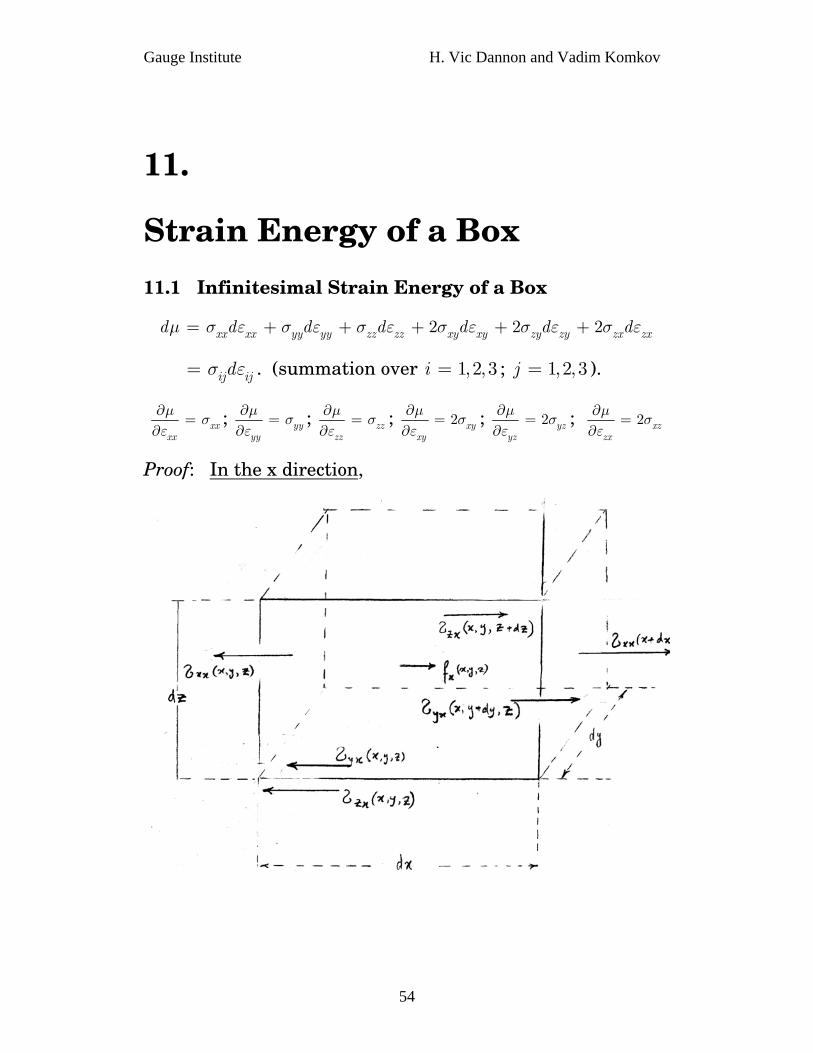
Strain Energy of a Box 11.1 Infinitesimal Strain Energy of a Box
2 2 2xx xx yy yy zz zz xy xy zy zy zx zxd d d d d d dμ σ ε σ ε σ ε σ ε σ ε σ ε= + + + + +
. (summation over ; ). ij ijdσ ε= 1,2,3i = 1,2,3j =
xxxx
μσ
ε∂
=∂
; yyyy
μσ
ε∂
=∂
; zzzz
μσ
ε∂
=∂
; 2 xyxy
μσ
ε∂
=∂
; 2 yzyz
μσ
ε∂
=∂
; 2 xzzx
μσ
ε∂
=∂
Proof: In the x direction,
54
Gauge Institute H. Vic Dannon and Vadim Komkov
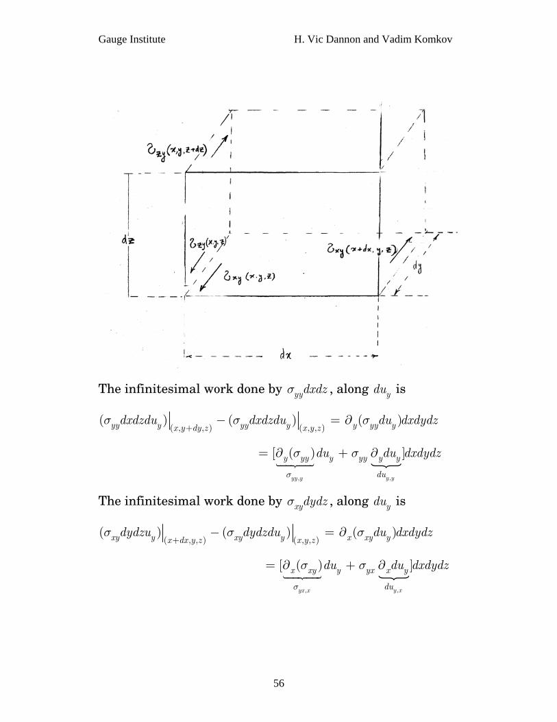
The infinitesimal work done by , along is xxdydzσ xdu
( , , ) ( , , )( ) ( ) ( )xx x xx x x xx xx dx y z x y zdydzdu dydzdu du dxdydzσ σ σ
+− = ∂
, ,
[ ( ) ]
xx x x x
x xx x xx x x
du
du du dxdydz
σ
σ σ= ∂ + ∂
The infinitesimal work done by , along is yxdydzσ xdu
( , , ) ( , , )( ) ( ) ( )yx x yx x y yx xx y dy z x y zdydzdu dxdzdu du dydxdzσ σ σ
+− = ∂
,,
[ ( ) ]
x yxy y
y yx x yx y x
du
du du dxdydz
σ
σ σ= ∂ + ∂
The infinitesimal work done by , along is zxdxdyσ xdu
( , , ) ( , , )( ) ( ) ( )zx x zx x z zx xx y z dz x y zdxdydu dxdydu du dydxdzσ σ σ
+− = ∂
,,
[ ( ) ]
x zxz z
z zx x zx z x
du
du du dxdydz
σ
σ σ= ∂ + ∂
The infinitesimal work done by ( , , )xf x y z dxdydz is
( , , )x xf x y z dxdydzdu .
In the y direction,
55
Gauge Institute H. Vic Dannon and Vadim Komkov
The infinitesimal work done by , along is yydxdzσ ydu
( , , ) ( , , )( ) ( ) ( )yy y yy y y yy yx y dy z x y zdxdzdu dxdzdu du dxdydzσ σ σ
+− = ∂
,,
[ ( ) ]
y yyy y
y yy y yy y y
du
du du dxdydz
σ
σ σ= ∂ + ∂
The infinitesimal work done by , along is xydydzσ ydu
( , , ) ( , , )( ) ( ) ( )xy y xy y x xy yx dx y z x y zdydzu dydzdu du dxdydzσ σ σ
+− = ∂
,,
[ ( ) ]
y xyx x
x xy y yx x y
du
du du dxdydz
σ
σ σ= ∂ + ∂
56

Gauge Institute H. Vic Dannon and Vadim Komkov
The infinitesimal work done by , along is zydxdyσ ydu
( , , ) ( , , )( ) ( ) ( )zy y zy y z zy yx y z dz x y zdxdydu dxdydu du dxdydzσ σ σ
+− = ∂
,,
[ ( ) ]
y zyz z
z zy y yz z y
du
du du dxdydz
σ
σ σ= ∂ + ∂
The work by ( , , )yf x y z dxdydz is ( , , )y yf x y z dxdydzdu .
In the z direction,
The infinitesimal work done by , along is zzdxdyσ zdu
( , , ) ( , , )( ) ( ) ( )zz z zz z z zz zx y z dz x y zdxdydu dxdzdu du dxdydzσ σ σ
+− = ∂
57
Gauge Institute H. Vic Dannon and Vadim Komkov
,,
[ ( ) ]
z zzz z
z zz z zz z z
du
du du dxdydz
σ
σ σ= ∂ + ∂
The infinitesimal work done by , along is zxdydzσ zdu
( , , ) ( , , )( ) ( ) ( )zx z zx z x zx zx dx y z x y zdydzu dydzdu du dxdydzσ σ σ
+− = ∂
,,
[ ( ) ]
z xzx x
x zx z zx x z
du
du du dxdydz
σ
σ σ= ∂ + ∂
The infinitesimal work done by , along is zydxdzσ zdu
( , , ) ( , , )( ) ( ) ( )zy z zy z y zy zx y dy z x y zdxdzdu dxdzdu du dxdydzσ σ σ
+− = ∂
,,
[ ( ) ]
z yyz z
y zy y yz y z
du
du du dxdydz
σ
σ σ= ∂ + ∂
The work by ( , , )zf x y z dxdydz is ( , , )z zf x y z dxdydzdu .
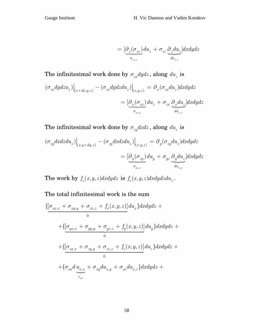
The total infinitesimal work is the sum
, , ,
0
{[ ( , , )] }xx x xy y xz z x xf x y z du dxdydzσ σ σ+ + + +
, , ,
0
{[ ( , , )] }yx x yy y yz z y yf x y z du dxdydzσ σ σ+ + + + +
, , ,
0
{[ ( , , )] }zx x zy y zz z z zf x y z du dxdydzσ σ σ+ + + + +
+
, , ,{ }
xx
xx x x xy x y xz x zd u du du dxdydz
ε
σ σ σ+ + +
58

Gauge Institute H. Vic Dannon and Vadim Komkov
, , ,{ }
yy
yy y y yx y x yz y zd u du du dxdydz
ε
σ σ σ+ + + +
ydz
, , , ,{ }
zz
zz z z zy z y z x z xd u du du dxdydz
ε
σ σ σ+ + +
{ }xx xx yy yy zz zzd d d dxdσ ε σ ε σ ε= + +
, , , , , ,
2 2 2
{ }
xy xy yz yz zx zx
xy x y yx y x yz y z zy z y zx z x xz x z
d d d
du du du du du du dxdydz
σ ε σ ε σ ε
σ σ σ σ σ σ+ + + + + +
The Infinitesimal work is stored in the box as Strain Energy.
The Infinitesimal Strain Energy per unit volume is
2 2 2xx xx yy yy zz zz xy xy yz yz zx zxd d d d d d dμ σ ε σ ε σ ε σ ε σ ε σ ε= + + + + + .
Hence,
xxxx
μσ
ε∂
=∂
; yyyy
μσ
ε∂
=∂
; zzzz
μσ
ε∂
=∂
;
2 xyxy
μσ
ε∂
=∂
; 2 yzyz
μσ
ε∂
=∂
; 2 xzzx
μσ
ε∂
=∂
.
11.2 Strain Energy density of a Box
1 1 12 2 2xx xx yy yy zz zz xy xy yz yz zx zxμ σ ε σ ε σ ε σ ε σ ε σ ε= + + + + + .
12 ij ijσ ε= . (summation over ). , 1,2,i j = 3
(1 ) 2 2 212 (1 )(1 2 ) (1 )(1 2 )
( ) {E Exx yy zz xx yy yy zz zz xx
ν νν ν ν ν
ε ε ε ε ε ε ε ε ε−+ − + −
= + + + + + } +
. 2 2 22 ( )xy yz zxG ε ε ε+ + +
59

Gauge Institute H. Vic Dannon and Vadim Komkov
Proof:
2 2 2xx xx yy yy zz zz xy xy yz yz zx zxd d d d d d dμ σ ε σ ε σ ε σ ε σ ε σ ε= + + + + +
Substituting
(1 )(1 2 )[(1 ) ]E
xx xx yy zzν νσ ν ε νε
+ −= − + + νε ,
(1 )(1 2 )[ (1 )E
yy xx yy zzν νσ νε ν ε
+ −= + − ]νε+ ,
(1 )(1 2 )[ (1E
zz xx yy zzν νσ νε νε
+ −= + + ) ]ν ε− ,
1E
xy xyνσ ε
+= ,
1E
yz yzνσ ε
+= ,
1E
zx zxνσ ε
+= .
(1 )(1 2 )[(1 ) ]E
xx yy zz xxd dν ν
μ ν ε νε νε+ −
= − + + ε +
(1 )(1 2 )
[ (1 ) ]Exx yy zz yydν ν
νε ν ε νε ε+ −
+ + − + +
(1 )(1 2 )
[ (1 ) ]Exx yy zz zzdν ν
νε νε ν ε ε+ −
+ + + − +
1 1 1
2 2 2E E Exy xy yz yz zx zxd d
ν ν νε ε ε ε ε ε
+ + ++ + + d .
(1 ) 2 2 212 (1 )(1 2 )
( )Exx yy zzdν
ν νε ε ε−
+ −= + + +
(1 )(1 2 )( )( ) ( )
{[ ] [ ] [ ]}
zz xxxx yy yy zz
Eyy xx xx yy yy zz zz yy zz xx xx zz
dd d
d d d d d dνν ν
ε εε ε ε ε
ε ε ε ε ε ε ε ε ε ε ε ε+ −
+ + + + + + +
2 2 21
2
( )Exy yz zx
G
dν
ε ε ε+
+ + + .
60
Gauge Institute H. Vic Dannon and Vadim Komkov
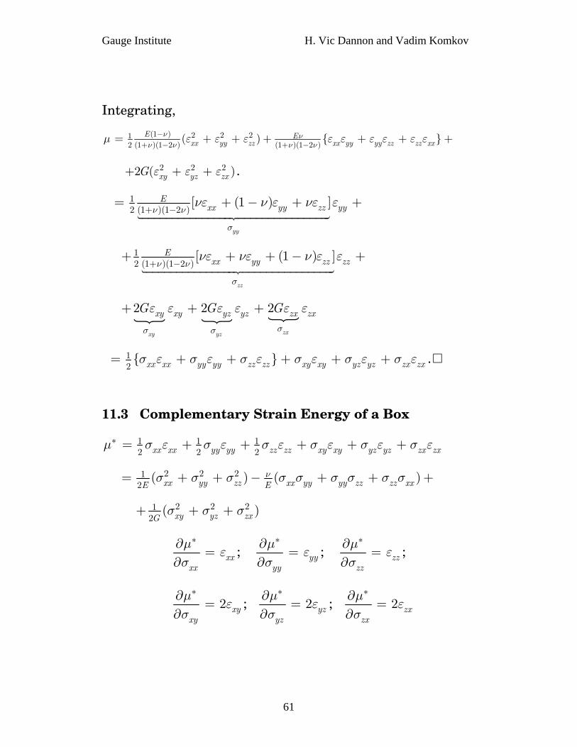
Integrating,
(1 ) 2 2 212 (1 )(1 2 ) (1 )(1 2 )
( ) {E Exx yy zz xx yy yy zz zz xx
ν νν ν ν ν
μ ε ε ε ε ε ε ε ε−+ − + −
= + + + + + }ε +
. 2 2 22 ( )xy yz zxG ε ε ε+ + +
12 (1 )(1 2 )
[ (1 ) ]
yy
Exx yy zz yyν ν
σ
νε ν ε νε ε+ −
= + − + +
12 (1 )(1 2 )
[ (1 )
zz
Exx yy zz zzν ν
σ
νε νε ν ε ε+ −
+ + + − ] +
2 2 2
zxxy yz
xy xy yz yz zx zxG G G
σσ σ
ε ε ε ε ε ε+ + +
12{ }xx xx yy yy zz zz xy xy yz yz zx zxσ ε σ ε σ ε σ ε σ ε σ ε= + + + + + .
11.3 Complementary Strain Energy of a Box
1 1 12 2 2xx xx yy yy zz zz xy xy yz yz zx zxμ σ ε σ ε σ ε σ ε σ ε σ ε∗ = + + + + +
2 2 212
( ) (xx yy zz xx yy yy zz zz xxE Eνσ σ σ σ σ σ σ σ σ= + + − + + )+
2 2 212
( )xy yz zxGσ σ σ+ + +
xxxx
με
σ
∗∂=
∂; yy
yy
με
σ
∗∂=
∂; zz
zz
με
σ
∗∂=
∂;
2 xyxy
με
σ
∗∂=
∂; 2 yz
yz
με
σ
∗∂=
∂; 2 zx
zx
με
σ
∗∂=
∂
61
Gauge Institute H. Vic Dannon and Vadim Komkov
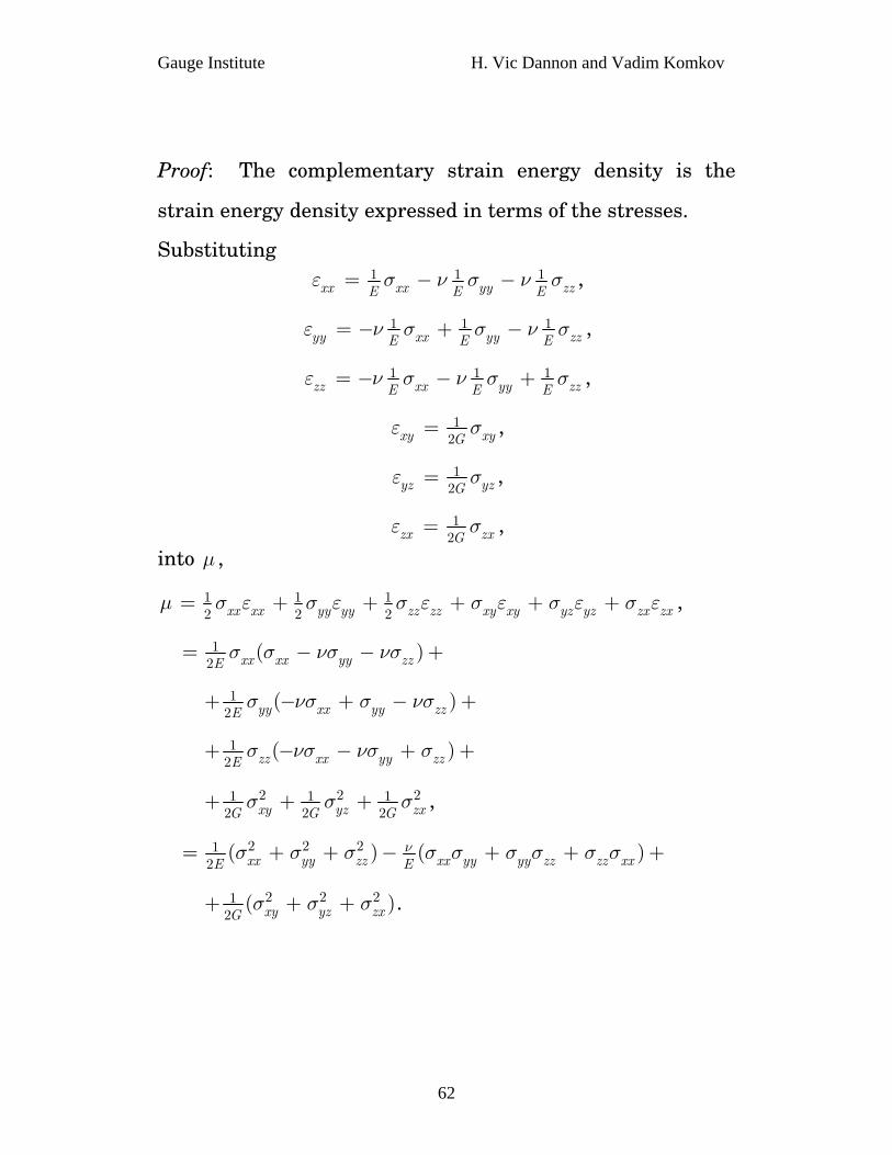
Proof: The complementary strain energy density is the
strain energy density expressed in terms of the stresses.
Substituting 1 1 1
xx xx yy zzE E Eε σ ν σ ν σ= − − ,
1 1 1yy xx yy zzE E Eε ν σ σ ν= − + − σ ,
1 1 1zz xx yy zzE E Eε ν σ ν σ= − − + σ ,
12xy xyG
ε σ= ,
12yz yzG
ε σ= ,
12zx zxG
ε σ= ,
into μ ,
1 1 12 2 2xx xx yy yy zz zz xy xy yz yz zx zxμ σ ε σ ε σ ε σ ε σ ε σ ε= + + + + + ,
12
( )xx xx yy zzEσ σ νσ νσ= − − +
12
( )yy xx yy zzEσ νσ σ νσ+ − + − +
12
( )zz xx yy zzEσ νσ νσ σ+ − − + +
2 21 1 12 2 2xy yz zxG G G
σ σ+ + + 2σ ,
2 2 212
( ) (xx yy zz xx yy yy zz zz xxE Eνσ σ σ σ σ σ σ σ σ= + + − + + )+
2 2 212
( )xy yz zxGσ σ σ+ + + .
62
Gauge Institute H. Vic Dannon and Vadim Komkov
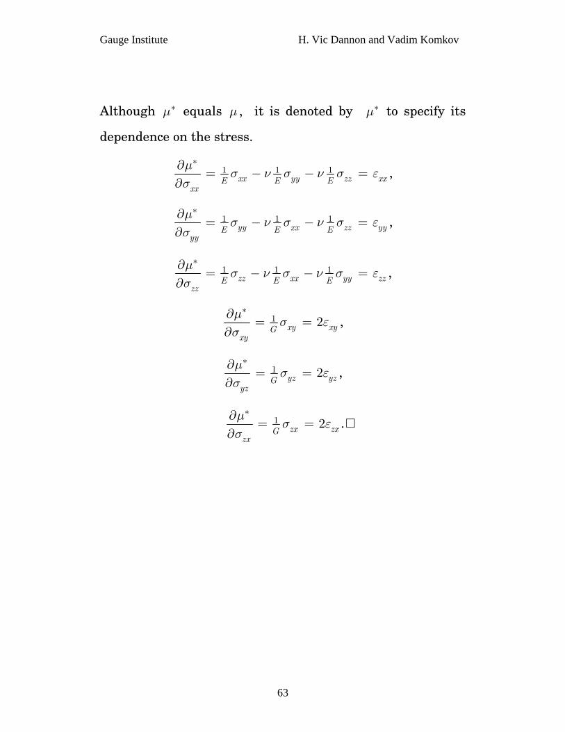
Although equals , it is denoted by μ to specify its
dependence on the stress.
μ∗ μ ∗
1 1 1xx yy zz xxE E E
xx
μσ ν σ ν σ ε
σ
∗∂= − − =
∂,
1 1 1yy xx zz yyE E E
yy
μσ ν σ ν σ ε
σ
∗∂= − − =
∂,
1 1 1zz xx yy zzE E E
zz
μσ ν σ ν σ ε
σ
∗∂= − − =
∂,
1 2xy xyGxy
μσ ε
σ
∗∂= =
∂,
1 2yz yzGyz
μσ ε
σ
∗∂= =
∂,
1 2zx zxGzx
μσ ε
σ
∗∂= =
∂.
63

Gauge Institute H. Vic Dannon and Vadim Komkov
12.
Variational Principles on a Box
12.1 Euler’s Variational Equations
The deflections , , and th at minimize or
maximize
xu yu zu
the box energy per unit volume,
( , , , , , , , , , , , )x y z xx yy zz xy yz zxF F x y z u u u ε ε ε ε ε ε=
satisfy Euler’s Variational Equation
( , , , , , , , , , , , ) 0x y z xx yy zz xy yz zxF x y z u u uδ ε ε ε ε ε =ε ,
which is,
1 12 2x y z
x xx xy xz
F F F Fu
uδ
ε ε ε
⎛ ⎞∂ ∂ ∂ ∂ ⎟⎜ ⎟⎜ − ∂ − ∂ − ∂ +⎟⎜ ⎟⎟⎜ ∂ ∂ ∂ ∂⎝ ⎠x
1 12 2x y z
y yx yy yz
F F F Fu
uδ
ε ε ε
⎛ ⎞∂ ∂ ∂ ∂ ⎟⎜ ⎟⎜+ − ∂ − ∂ − ∂ ⎟⎜ ⎟⎟⎜∂ ∂ ∂ ∂⎝ ⎠y +
1 12 2
0x y z zz zx zy zz
F F F Fu
uδ
ε ε ε
⎛ ⎞∂ ∂ ∂ ∂ ⎟⎜ ⎟⎜+ − ∂ − ∂ − ∂ =⎟⎜ ⎟⎟⎜∂ ∂ ∂ ∂⎝ ⎠.
or,
1 12 2
0x y zx xx xy xz
F F F Fu ε ε ε∂ ∂ ∂ ∂
− ∂ − ∂ − ∂ =∂ ∂ ∂ ∂
,
64
Gauge Institute H. Vic Dannon and Vadim Komkov
1 12 2
0x y zy yx yy yz
F F F Fu ε ε ε
∂ ∂ ∂ ∂− ∂ − ∂ − ∂ =
∂ ∂ ∂ ∂,
1 12 2
0x y zz zx zy zz
F F F Fu ε ε ε
∂ ∂ ∂ ∂− ∂ − ∂ − ∂ =
∂ ∂ ∂ ∂.
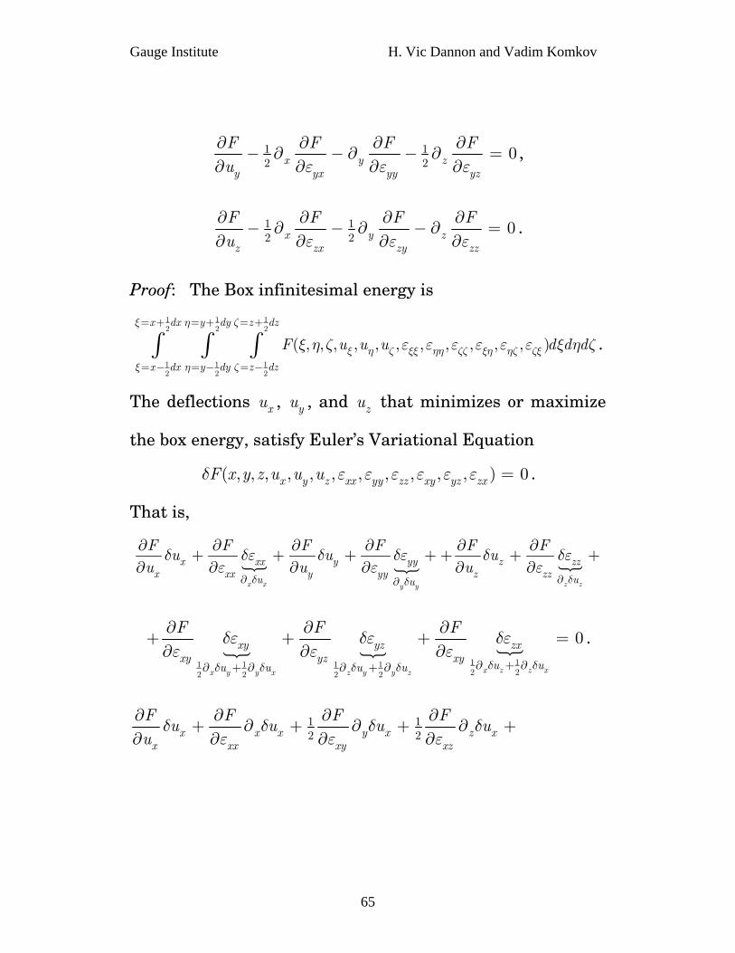
Proof: The Box infinitesimal energy is 1 1 12 2 2
1 1 12 2 2
( , , , , , , , , , , , )
x dx y dy z dz
x dx y dy z dz
F u u u d d
ξ η ζ
ξ η ζ ξξ ηη ζζ ξη ηζ ζξξ η ζ
ξ η ζ ε ε ε ε ε ε ξ η ζ= + = + = +
= − = − = −∫ ∫ ∫ d
ε
.
The deflections , , and that minimizes or maximize
the box energy, satisfy Euler’s Variational Equation
xu yu zu
( , , , , , , , , , , , ) 0x y z xx yy zz xy yz zxF x y z u u uδ ε ε ε ε ε = .
That is,
x x z zy y
x xx y yy zx xx y yy z zzu uu
F F F F F Fu u u
u u uδ δδ
δ δε δ δε δ δεε ε
∂ ∂∂
∂ ∂ ∂ ∂ ∂ ∂+ + + + + +
∂ ∂ ∂ ∂ ∂ ∂ zzε+
1 11 1 1 12 22 2 2 2
0
x z z xx y y x z y y z
xy yz zxxy yz xy
u uu u u u
F F F
δ δδ δ δ δ
δε δε δεε ε ε
∂ + ∂∂ + ∂ ∂ + ∂
∂ ∂ ∂+ + +∂ ∂ ∂
= .
1 12 2x x x y x z
x xx xy xz
F F F Fu u u
uδ δ δ
ε ε ε∂ ∂ ∂ ∂
+ ∂ + ∂ + ∂∂ ∂ ∂ ∂ xuδ +
65
Gauge Institute H. Vic Dannon and Vadim Komkov
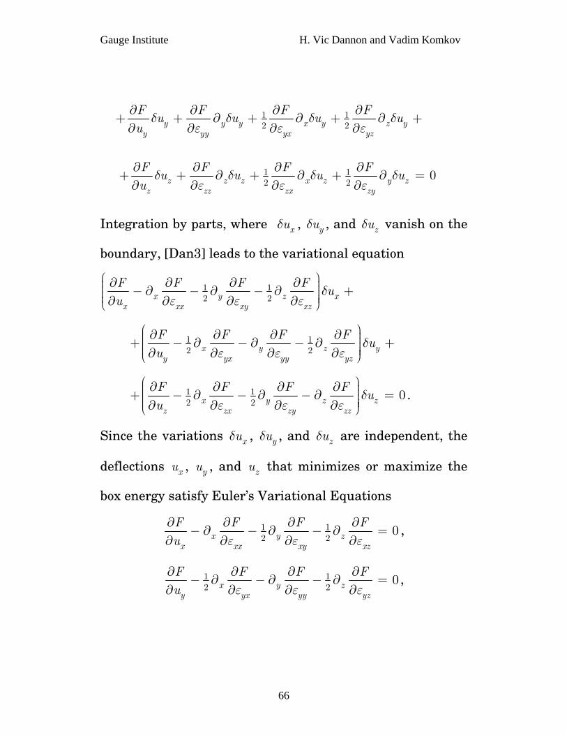
1 12 2y y y x y z
y yy yx yz
F F F Fu u u
uδ δ δ
ε ε ε∂ ∂ ∂ ∂
+ + ∂ + ∂ + ∂∂ ∂ ∂ ∂ yuδ +
1 12 2
0z z z x z y zz zz zx zy
F F F Fu u u u
uδ δ δ δ
ε ε ε∂ ∂ ∂ ∂
+ + ∂ + ∂ + ∂∂ ∂ ∂ ∂
=
Integration by parts, where , , and vanish on the
boundary, [Dan3] leads to the variational equation
xuδ yuδ zuδ
1 12 2x y z
x xx xy xz
F F F Fu
uδ
ε ε ε
⎛ ⎞∂ ∂ ∂ ∂ ⎟⎜ ⎟⎜ − ∂ − ∂ − ∂ +⎟⎜ ⎟⎟⎜ ∂ ∂ ∂ ∂⎝ ⎠x
1 12 2x y z
y yx yy yz
F F F Fu
uδ
ε ε ε
⎛ ⎞∂ ∂ ∂ ∂ ⎟⎜ ⎟⎜+ − ∂ − ∂ − ∂ ⎟⎜ ⎟⎟⎜∂ ∂ ∂ ∂⎝ ⎠y +
1 12 2
0x y z zz zx zy zz
F F F Fu
uδ
ε ε ε
⎛ ⎞∂ ∂ ∂ ∂ ⎟⎜ ⎟⎜+ − ∂ − ∂ − ∂ =⎟⎜ ⎟⎟⎜∂ ∂ ∂ ∂⎝ ⎠.
Since the variations , , and are independent, the
deflections , , and that minimizes or maximize the
box energy satisfy Euler’s Variational Equations
xuδ yuδ zuδ
xu yu zu
1 12 2
0x y zx xx xy xz
F F F Fu ε ε ε∂ ∂ ∂ ∂
− ∂ − ∂ − ∂ =∂ ∂ ∂ ∂
,
1 12 2
0x y zy yx yy yz
F F F Fu ε ε ε
∂ ∂ ∂ ∂− ∂ − ∂ − ∂ =
∂ ∂ ∂ ∂,
66

Gauge Institute H. Vic Dannon and Vadim Komkov
1 12 2
0x y zz zx zy zz
F F F Fu ε ε ε
∂ ∂ ∂ ∂− ∂ − ∂ − ∂ =
∂ ∂ ∂ ∂.
12.2 If the body forces originate from a Potential ( , , )x y zu u uυ
per unit volume, so that
xx
fuυ∂
− =∂
,
yy
fuυ∂
− =∂
,
zz
fuυ∂
− =∂
,
Then, Euler’s Equations are the Equilibrium Equations
, , , 0xx x xy y xz z xfσ σ σ+ + + = ,
, , , 0yx x yy y yz z yfσ σ σ+ + + = ,
, , , 0zx x zy y zz z zfσ σ σ+ + + = .
Proof: The Energy per unit volume is
( , , , , , , , , , , , )x y z xx yy zz xy yz zxF x y z u u u ε ε ε ε ε ε μ υ= +
1 1 12 2 2xx xx yy yy zz zz xy xy yz yz zx zxσ ε σ ε σ ε σ ε σ ε σ ε υ= + + + + + + .
The Euler’s Variational Equations are
67
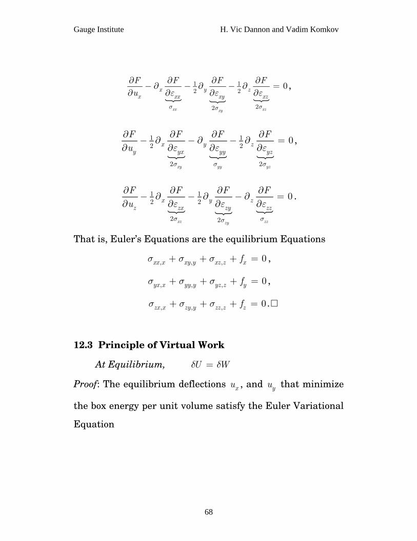
Gauge Institute H. Vic Dannon and Vadim Komkov
1 12 2
22
0
xx xzxy
x y zx xx xy xz
F F F Fu
σ σσ
ε ε ε∂ ∂ ∂ ∂
− ∂ − ∂ − ∂ =∂ ∂ ∂ ∂
,
1 12 2
2 2
0
xy yy yz
x y zy yx yy yz
F F F Fu
σ σ σ
ε ε ε∂ ∂ ∂ ∂
− ∂ − ∂ − ∂ =∂ ∂ ∂ ∂
,
1 12 2
2 2
0
xz zzzy
x y zz zx zy zz
F F F Fu
σ σσ
ε ε ε∂ ∂ ∂ ∂
− ∂ − ∂ − ∂ =∂ ∂ ∂ ∂
.
That is, Euler’s Equations are the equilibrium Equations
, , , 0xx x xy y xz z xfσ σ σ+ + + = ,
, , , 0yx x yy y yz z yfσ σ σ+ + + = ,
, , , 0zx x zy y zz z zfσ σ σ+ + + = .
12.3 Principle of Virtual Work
At Equilibrium, U Wδ δ=
Proof: The equilibrium deflections , and that minimize
the box energy per unit volume satisfy the Euler Variational
Equation
xu yu
68
Gauge Institute H. Vic Dannon and Vadim Komkov
1 12 2x y z
x xx xy xz
F F F FF u
uδ δ
ε ε ε
⎛ ⎞∂ ∂ ∂ ∂ ⎟⎜ ⎟⎜= − ∂ − ∂ − ∂ ⎟⎜ ⎟⎟⎜∂ ∂ ∂ ∂⎝ ⎠x +
1 12 2x y z
y yx yy yz
F F F Fu
uδ
ε ε ε
⎛ ⎞∂ ∂ ∂ ∂ ⎟⎜ ⎟⎜+ − ∂ − ∂ − ∂ ⎟⎜ ⎟⎟⎜∂ ∂ ∂ ∂⎝ ⎠y +
1 12 2
0x y z zz zx zy zz
F F F Fu
uδ
ε ε ε
⎛ ⎞∂ ∂ ∂ ∂ ⎟⎜ ⎟⎜+ − ∂ − ∂ − ∂ =⎟⎜ ⎟⎟⎜∂ ∂ ∂ ∂⎝ ⎠.
Thus, at equilibrium, the Variation of F , [Dan3], satisfies
0.Fδ =
Therefore,
( )U W U Wδ δ δ− = −
0 0 0
( , , , , , , , , , , , )yx z
y lx l z l
x y z xx yy zz xy yz zxx y z
F x y z u u u dxdydzδ ε ε ε ε ε ε== =
= = =
= ∫ ∫ ∫
0 0 0
( , , , , , , , , , , , )yx z
y lx l z l
x y z xx yy zz xy yz zxx y z
F x y z u u u dxdydzδ ε ε ε ε ε ε== =
= = =
= ∫ ∫ ∫
. 0=
That is, . U Wδ δ=
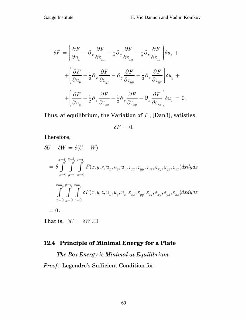
12.4 Principle of Minimal Energy for a Plate
The Box Energy is Minimal at Equilibrium
Proof: Legendre’s Sufficient Condition for
69
Gauge Institute H. Vic Dannon and Vadim Komkov
0 0 0
( , , , , , , , , , , , )yx z
y lx l z l
x y z xx yy zz xy yz zxx y z
F x y z u u u dxdydzε ε ε ε ε ε== =
= = =∫ ∫ ∫
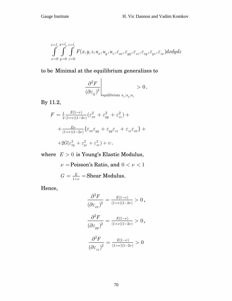
to be Minimal at the equilibrium generalizes to
2
2equilibrium ; ;
0( )
x y zij u u u
F
ε
∂>
∂.
By 11.2,
(1 ) 2 2 212 (1 )(1 2 )
( )Exx yy zzF ν
ν νε ε ε−
+ −= + + +
(1 )(1 2 )
{ }Exx yy yy zz zz xx
νν ν
ε ε ε ε ε ε+ −
+ + + +
υ
. 2 2 22 ( )xy yz zxG ε ε ε+ + + +
where is Young’s Elastic Modulus, 0E >
ν Poisson’s Ratio, and = 0 1ν< <
1EGν+
= =Shear Modulus.
Hence, 2
(1 )
(1 )(1 2 )20
( )E
xx
F νν νε
−+ −
∂= >
∂,
2(1 )
(1 )(1 2 )20
( )E
yy
F νν νε
−+ −
∂= >
∂,
2(1 )
(1 )(1 2 )20
( )E
zz
F νν νε
−+ −
∂= >
∂
70
Gauge Institute H. Vic Dannon and Vadim Komkov
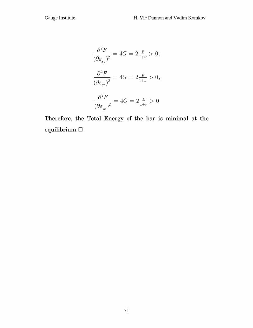
2
124 2
( )E
xy
FG
νε +
∂= = >
∂0 ,
2
124 2
( )E
yz
FG
νε +
∂= = >
∂0 ,
2
124 2
( )E
zx
FG
νε +
∂= = >
∂0
Therefore, the Total Energy of the bar is minimal at the
equilibrium.
71
Gauge Institute H. Vic Dannon and Vadim Komkov
13.
Castigliano Theorems There are infinitely many body forces applying to the
infinitely many material particles of an elastic structure.
In Engineering, those many forces are replaced by several
forces concentrated and at their points of application in the
structure.
Then, Castigliano Theorem for the Displacements yields the
displacements as the derivatives of the complementary
strain energy with respect to the forces at the application
points.
And Castigliano Theorem for the Forces yields the forces as
the derivatives of the strain energy with respect to the
displacements at the application points.
13.1 Castigliano Theorem for the Displacements
If an elastic structure is at equilibrium under concentrated
Body Forces
1P , ,… 2P
applied at several points
72
Gauge Institute H. Vic Dannon and Vadim Komkov
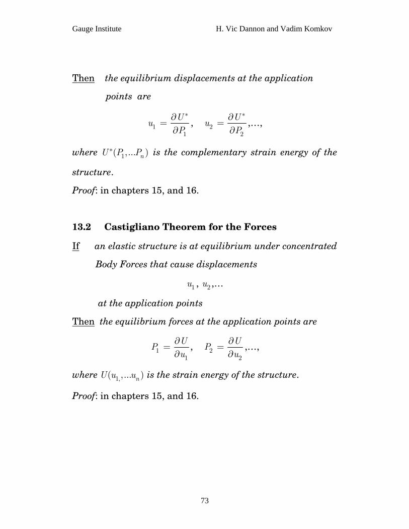
Then the equilibrium displacements at the application
points are
11
Uu
P
∗∂=
∂, 2
2
Uu
P
∗∂=
∂,…,
where is the complementary strain energy of the
structure.
1( ,... )nU P P∗
Proof: in chapters 15, and 16.
13.2 Castigliano Theorem for the Forces
If an elastic structure is at equilibrium under concentrated
Body Forces that cause displacements
1u , ,… 2u
at the application points
Then the equilibrium forces at the application points are
11
UP
u∂
=∂
, 22
UP
u∂
=∂
,…,
where is the strain energy of the structure. 1,( ,... )nU u u
Proof: in chapters 15, and 16.
73
Gauge Institute H. Vic Dannon and Vadim Komkov
14.
Erroneous Derivations of
Castigliano Theorems
Castigliano Theorems follow from the Variational Principles
of Elasticity. They can be derived from the Principle of
Virtual Work, or from the Principle of Minimal Potential.
Attempting to prove them otherwise may fail.
The following erroneous derivation appears in [Timoshenko],
and is followed by [Mura].
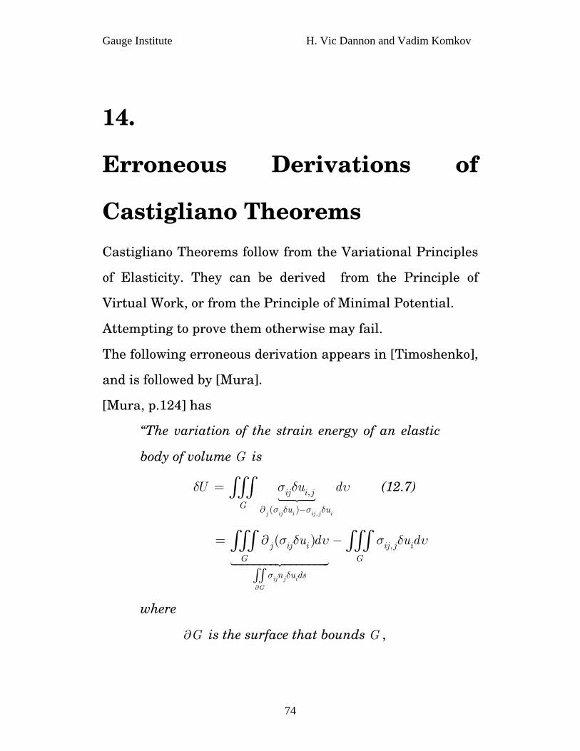
[Mura, p.124] has
“The variation of the strain energy of an elastic
body of volume G is
,
,
( )j ij i ij j i
ij i jG u u
U u
σ δ σ δ
δ σ δ
∂ −
= ∫∫∫ dυ (12.7)
,( )
ij j iG
j ij i ij j iG G
n u ds
u d u d
σ δ
σ δ υ σ δ υ
∂
= ∂ −
∫∫
∫∫∫ ∫∫∫
where
is the surface that bounds G , G∂
74
Gauge Institute H. Vic Dannon and Vadim Komkov
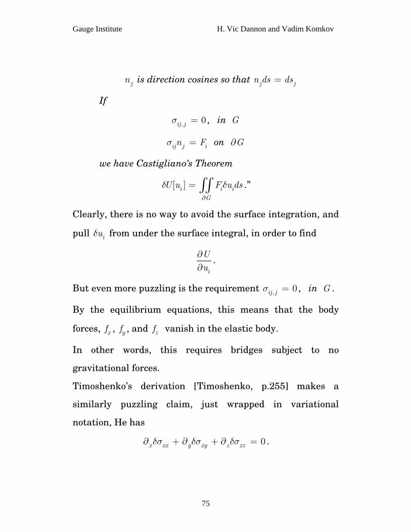
is direction cosines so that jn j jn ds ds=
If
, 0ij jσ = , in G
ij j inσ = F
i
on G∂
we have Castigliano’s Theorem
[ ]i iG
U u F u dsδ δ∂
= ∫∫ .”
Clearly, there is no way to avoid the surface integration, and
pull from under the surface integral, in order to find iuδ
i
Uu
∂∂
.
But even more puzzling is the requirement , in G . , 0ij jσ =
By the equilibrium equations, this means that the body
forces, xf , yf , and zf vanish in the elastic body.
In other words, this requires bridges subject to no
gravitational forces.
Timoshenko’s derivation [Timoshenko, p.255] makes a
similarly puzzling claim, just wrapped in variational
notation, He has
0x xx y xy z xzδσ δσ δσ∂ + ∂ + ∂ = .
75
Gauge Institute H. Vic Dannon and Vadim Komkov
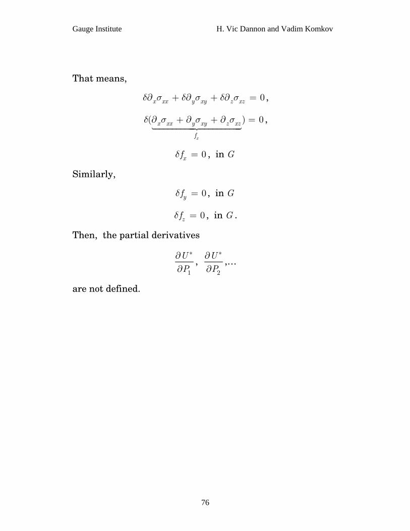
That means,
0x xx y xy z xzδ σ δ σ δ σ∂ + ∂ + ∂ = ,
( )
x
x xx y xy z xz
f
δ σ σ σ∂ + ∂ + ∂ = 0 ,
0xfδ = , in G
Similarly,
0yfδ = , in G
0zfδ = , in G .
Then, the partial derivatives
1
UP
∗∂∂
, 2
UP
∗∂∂
,…
are not defined.
76

Gauge Institute H. Vic Dannon and Vadim Komkov
15.
Castigliano Theorems and the
Principle of Virtual Work
15.1 Proof of Castigliano Theorem for Forces
If under several concentrated body forces applied at several
points, the strain energy U depends on the displacements,
1( ,... )nU U u u= ,
the infinitesimal work along ,…. is 1uδ nuδ
1 1 ... n nW P u P uδ δ= + + δ .
By the Principle of Virtual Work,
1 1 ... n nU W P u P uδ δ δ δ= = + +
Therefore,
11
UP
u∂
=∂
,… nn
UP
u∂
=∂
.
15.2 Proof of Castigliano Theorem for Displacements
77

Gauge Institute H. Vic Dannon and Vadim Komkov
If under several concentrated body forces applied at several
points, the Complementary Strain energy U depends on the
Forces,
∗
1( ,... )nU U P P∗ ∗= ,
the infinitesimal work by ,…. is 1Pδ nPδ
1 1 ... n nW u P uδ δ∗ = + + Pδ
P
.
By the Principle of Virtual Work,
1 1 ... n nU W u P uδ δ δ δ∗ ∗= = + +
Therefore,
11
Uu
P
∗∂=
∂,… n
n
Uu
P
∗∂=
∂.
78

Gauge Institute H. Vic Dannon and Vadim Komkov
16.
Castigliano Theorems and the
Hamiltonian
16.1 The Hamiltonian of Concentrated Forces
is the potential
1 1 1 1( ,... , ,... ) ....n n nP P u u U Pu P uΗ = − − n−
where
1 1( ,... ) ( ,... )n nU U u u U P P∗= =
16.2 Castigliano Theorem for the Forces is Hamilton’s
Equations
ii
UP
u∂
=∂
Proof: By the Principle of Minimal Potential, 0iu
∂Η=
∂.
79
Gauge Institute H. Vic Dannon and Vadim Komkov
16.3 Castigliano Theorem for the displacements is
Hamilton’s Equations
ii
UP
u∂
=∂
Proof: By the Principle of Minimal Potential, 0iP
∂Η=
∂.
80
Gauge Institute H. Vic Dannon and Vadim Komkov
17.
Castigliano and Beam Bending
without Shear
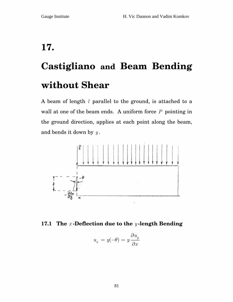
A beam of length l parallel to the ground, is attached to a
wall at one of the beam ends. A uniform force P pointing in
the ground direction, applies at each point along the beam,
and bends it down by y .
17.1 The x -Deflection due to the y -length Bending
( ) yx
uu y y
xθ
∂= − =
∂
81
Gauge Institute H. Vic Dannon and Vadim Komkov
Proof: ( ) xx
uu y y
yθ
⎛ ⎞∂ ⎟⎜ ⎟= − = −⎜ ⎟⎜ ⎟∂⎝ ⎠
Zero shear means that 0y xu u
x y
∂ ∂+ =
∂ ∂, Therefore,
yx
uu y
x
∂=
∂
17.2 The x -Strain due to the y -length Bending
2
20
yxx
y
uyx
ε=
⎛ ⎞⎟∂⎜ ⎟⎜ ⎟= ⎜ ⎟⎜ ⎟∂⎜ ⎟⎟⎜⎝ ⎠.
17.3 The x -Stress due to the y -length Bending
2
20
yxx
y
uEy
xσ
=
⎛ ⎞⎟∂⎜ ⎟⎜ ⎟= ⎜ ⎟⎜ ⎟∂⎜ ⎟⎟⎜⎝ ⎠.
17.4 The Bending Moment at , x
( )M x Px=2
22
0
y
AyI
uE y d
x=
∂=
∂ ∫∫ A
where I is the Inertia Moment.
Proof:
82

Gauge Institute H. Vic Dannon and Vadim Komkov
( ) xxA
M x ydAσ= ∫∫
2
22
0
y
A y
uEy dA
x=
∂=
∂∫∫
2
22
0
y
AyI
uE y d
x=
∂=
∂ ∫∫ A .
17.5 The x -Stress due to the y -length Bending
( )xx
M xy
Iσ = .
Proof: 2
20
( ) ( )y
y
u M x M xEy Ey y
EI Ix=
⎛ ⎞⎟∂⎜ ⎟⎜ ⎟ = =⎜ ⎟⎜ ⎟∂⎜ ⎟⎟⎜⎝ ⎠.
17.6 The Strain Energy of the Bending at x l , =
2
0
1( ) ( )
2
x l
x
U l M x dxEI
=
=
= ∫
Proof: 2
0
12
x l
xxx A
U dE
σ=
=
= ∫ ∫∫ Adx
83
Gauge Institute H. Vic Dannon and Vadim Komkov
2
0
1 ( )2
x l
x A
M xy dAdx
E I
=
=
⎛ ⎞⎟⎜= ⎟⎜ ⎟⎟⎜⎝ ⎠∫ ∫∫
2 22
0
1( )
2
x l
x A
I
M x y dAdxEI
=
=
= ∫ ∫∫
2
0
1( )
2
x l
x
M x dxEI
=
=
= ∫ .
17.7 The vertical deflection at x is l=3
3PlEI
Proof: By Castigliano, the vertical deflection at x is l=
2
0
( ) 1( )
2
x l
Px
U lM x dx
P EI
=
=
∂= ∂
∂ ∫
2
0
1( )
2
x l
Px
M x dxEI
=
=
= ∂∫
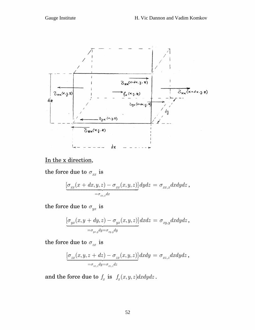
0
12 (
2
x l
PPxx x
M M x dEI
=
=
= ∂∫ ) x
3
2
03
x l
x
P Px dx
EI EI
=
=
= =∫l .
84
Gauge Institute H. Vic Dannon and Vadim Komkov
17.8 The deflection angel is 2
2PlEI
Proof: By Castigliano, the deflection angel is
2
0
( ) 1( )
2
x l
Mx
U lM x dx
M EI
=
=
∂= ∂
∂ ∫
2
0
1( )
2
x l
Mx
M x dxEI
=
=
= ∂∫
0
12
2
x l
Pxx
MdxEI
=
=
= ∫
2
02
x l
x
P Pxdx
EI EI
=
=
= =∫l .
85

Gauge Institute H. Vic Dannon and Vadim Komkov
References
[Arthurs] Arthurs, A. M., “Calculus Of Variations”, Routledge, 1975.
[Byerly1] Byerly, William, Elwood, “Introduction to the Calculus of
Variations”, Harvard, 1933
[Byerly2] Byerly, William, Elwood, “An Introduction to the use of
Generalized Coordinates in Mechanics and Physics”, Dover, (1916 reprint)
[Chou] Pei Chi Chou, and Pagano, Nicholas, “Elasticity, Tensor, Dyadic, and
Engineering Approaches” Van Nostrand, 1967.
[Dan1] Dannon, H. Vic, “Infinitesimals” in Gauge Institute Journal Vol.6 No
4, November 2010;
[Dan2] Dannon, H. Vic, “Infinitesimal Calculus” in Gauge Institute Journal
Vol.7 No 4, November 2011
[Dan3] Dannon, H. Vic, “Infinitesimal Variational Calculus” in Gauge
Institute Journal Vol. No ,
[Elsgolts] Elsgolts, L. “Differential Equations and the Calculus of
Variations”, MIR, 1970.
[Forray] Forray, Marvin, “Variational Calculus in Science and Engineering”
McGraw-Hill, 1968.
[Forsyth] Forsyth, A. R., “Calculus of Variations”, Cambridge, 1927.
[Fox] Fox, Charles, “An Introduction to the calculus of Variations”, Oxford,
1950.
[Hancock] Hancock, Harris, “Lectures on the Calculus of Variations (The
Weierstrassian Theory)” University of Cincinnati, 1904.
[Hartog] Hartog, J. P. Den, “Strength of Materials” McGraw-Hill, 1949;
“Advanced Strength of Materials” McGraw-Hill, 1952.
86
Gauge Institute H. Vic Dannon and Vadim Komkov
[Komkov] Komkov Vadim, “Variational Principles of Continuum Mechanics
with Engineering Applications Volume 1: Critical Points Theory” Reidel,
1986, “Variational principles of Continuum Mechanics with Engineering
applications Volume 2: Introduction to Optimal Design Theory” Reidel, 1988,
[Mura] Mura, Toshio, & Koya, Tatsuhito, “Variational Methods in Mechanics”
Oxford, 1992.
[Pars] Pars, L. A., “An Introduction to the Calculus of Variations”,
Heinemann, 1962
[Pearson] Pearson, Carl, “Theoretical Elasticity”, Harvard U. Press, 1959
[Pilkey] Pilkey, Walter & Wunderlich Walter, “Mechanics of Structures,
Variational and Computational Methods”, CRC, 1994.
[Rand] Rand, Omri, & Rovenski, Vladimir, “Analytical Methods in
Anisotropic Elasticity with Symbolic Computational Tools” Birkhauser, 2005.
[Reddy] Reddy, J. N. “Energy Principles and variational Methods in Applied
Mechanics” Second Edition, Wiley, 2002
[Sagan] Sagan, Hans, “Introduction to the Calculus of Variations”, McGraw-
Hill, 1969.
[Timoshenko] Timoshenko, S. P. & Goodier, J. N. “Theory of Elasticity”
Third Edition, McGraw-Hill, 1970.
[Todhunter] Todhunter, I. “A History of the Calculus of Variations during
the nineteenth century” Chelsea, (1861 reprint)
[Wang] Wang, Chi-The, “Applied Elasticity” McGraw-Hill, 1953.
[Weinstock] Weinstock, Robert, “Calculus of Variations with Applications to
Physics and Engineering” McGraw-Hill, 1952.
87