Embed Size (px)
Citation preview

University of Washington Technical Report UW-CSE-12-10-01
Inferring Models of Networked Systemsfrom Logs of their Behavior with Dynoptic
Ivan BeschastnikhUniversity of Washington
Yuriy BrunUniversity of Massachusetts
Michael D. Ernst Arvind KrishnamurthyUniversity of Washington
{mernst,arvind}@cs.washington.edu
AbstractNetworked systems are notoriously difficult to debug and understand.A common way of gaining insight into system behavior is to inspectexecution logs and documentation. Unfortunately, manual inspectionof logs is an arduous process and documentation is often incompleteand out of sync with the implementation.
To provide developers with more insight into networked systems,we developed Dynoptic, a tool that infers a concise and accuratemodel of a system, in the form of a communicating finite state ma-chine from logs of the system’s behavior. Engineers can use theinferred models to understand complex behavior, detect anomalies,debug, and increase confidence in the correctness of their implemen-tations. Unlike most prior work, Dynoptic processes the logs mostsystems already produce and requires developers only to specify aset of regular expressions for parsing the logs. We formally describeDynoptic and present a preliminary evaluation on logs from threedifferent systems.
1. IntroductionWhen a system behaves in an unexpected manner or when adeveloper must make changes to code written by someone else, thedeveloper faces the challenging task of understanding the system’sbehavior. To help with this task, developers often enable loggingand analyze the logged system behavior. Unfortunately, the size andcomplexity of logs often exceed a human’s ability to navigate andmake sense of the captured data. For example, production systemsat Google log billions of events each day; these are stored for weeksto help diagnose errant future behaviors [42].
One promising approach to help developers make sense oflogs is model inference. The goal of a model inference algorithmis to convert a log of system executions into a model, typicallya finite state machine, that accurately and concisely representsthe system that generated the log. Numerous model inferencealgorithms and tools exist to help debug, verify, and validatesequential programs [6, 7, 28, 29, 31].
This rich prior body of work is not directly applicable to aconcurrent, distributed, or networked system. This is because acommon assumption made in model inference is that the underlyingset of executions is totally ordered — for every pair of events in anexecution, one precedes the other. This assumption does not hold fornetworked and distributed systems, in which events at differentnodes may occur without any happens-before relationship [27].Therefore the finite state machine (FSM) models that most inferencealgorithms infer are difficult or impossible to map back to the multi-process implementation that generated the log.
This paper describes a new model inference technique and acorresponding tool, called Dynoptic, which infers communicatingfinite state machine (CFSM) [10] models of the processes thatgenerated the log. Dynoptic can be applied to logs of distributed
systems, protocol traces, traces of AJAX events in a web-browser,and other behavior traces. Dynoptic models have multiple developer-oriented uses — developers can inspect, query, and check Dynoptic’smodels against their own mental model of the system. These uses arethe focus of our present work. However, we believe that Dynoptic-generated models have numerous other uses, such as model-basedtesting of networked systems, and detection of anomalous behavioras systems are exposed to new workloads or environments.
The Dynoptic prototype is available for download1. We presentresults from a preliminary evaluation of the prototype in whichDynoptic constructed models of the alternating bit protocol [37], theopening and closing handshake of the TCP protocol, and a portionof the replication strategy in the Voldemort [40] distributed hashtable.
The next section overviews the Dynoptic approach. Then, Sec-tion 3 formally defines the algorithm and Section 4 proves that itreturns models that are accurate, in the sense that they satisfy themined log properties we define. Section 5 presents an evaluationof the Dynoptic tool on logs generated by three systems. Section 6overviews related work, Section 7 discusses issues raised by ourwork, and Section 8 concludes.
2. Overview of the Dynoptic approachDynoptic’s input is a log of observed events, and its output is amodel that describes the distributed system that generated the log.An input log consists of execution traces of the system. A trace is aset of events, each of which has a vector timestamp [17, 32].
Vector time is a standard logical clock mechanism that providesa partial ordering of events. In a distributed system of h hosts, eachhost maintains an array of clocks, one clock for each host. Whengenerating an event, the host increments its own clock in the array.When sending a message to another host, the sender shares its clocksarray with the receiver, who updates its local clocks array to themost recent clock values (and increments its local clock, as messagereceipt is an event). The system maintains the vector time duringexecutions and appends a timestamp to each logged event.
Figure 1(a) shows an example input log generated by twoprocesses executing the alternating bit protocol [37]. In the protocol,a sender process communicates a sequence of messages to a receiverprocess over an unreliable channel. The protocol is stop-and-wait —the receiver must acknowledge an outstanding message before thesender moves on to the next message. If a message is delayed orlost, the sender re-transmits the message after a timeout.
Figure 1(b) shows Dynoptic’s output — a communicating finitestate machine [10] (CFSM) model — for a more complete log of thealternating bit protocol (not shown). A CFSM models multiple pro-cesses, or threads of execution, each of which is described by a finite
1 http://synoptic.googlecode.com
1

University of Washington Technical Report UW-CSE-12-10-01
M
A
s0 s1send(m) s2M!m-0
timeout
A?a-1
s3
A?a-0
s4 send(m)s5 M!m-1
A?a-1
A?a-0
timeout
(b.1) Output model (Sender)
A?a-1
r0 r1M?m-0 r2recv(m) M?m-0
r3r4 M?m-1r5 recv(m)
A!a-1
M?m-1
M?m-1 M?m-0 A!a-0
(b.2) Output model (Receiver)
1,02,03,34,35,36,67,68,69,910,911,912,12
(a) Input log
Sender ReceiverM?m-0recv(m)A!a-0M?m-1recv(m)A!a-1M?m-0recv(m)A!a-0M?m-1recv(m)A!a-1
2,12,22,35,45,55,68,78,88,9
11,1011,1111,12
send(m)M!m-0A?a-0send(m)M!m-1A?a-1send(m)M!m-0A?a-0send(m)M!m-1A?a-1
Figure 1: Example input and output of Dynoptic. (a) Example input log with a single vector-timestamped trace of two processes running the alternating bitprotocol (ABP) [37]. (b) The CFSM model of ABP derived by Dynoptic, with (b.1) the sender process model and (b.2) the receiver process model. Thesemodels were inferred by Dynoptic for this system on a more complete log (not shown).In ABP, the sender transmits messages to the receiver using channel M, and the receiver replies with acknowledgments through channel A. Notation Q!x meansenqueue message x at head of channel Q, and event Q?x means dequeue message x from the head of channel Q. The event send(m) is a down-call to send m atthe sender, and recv(m) is an up-call at the receiver indicating that m was received. The timeout event at the sender triggers a message re-transmission aftersome internal timeout threshold is reached. The “alternating bit” is associated with each message and is appended to a message’s channel representation as -0 or-1. For example, the first (and every odd) message sent by the sender is represented as m-0 and the corresponding response is represented as a-0.
state machine (FSM). In the standard CFSM formalism, processescommunicate with one another via message passing over reliableFIFO channels. However, unreliable channels can be simulated byreplacing each unreliable channel with a lossy “middlebox” FSMthat non-deterministically chooses between forwarding and losing amessage. The model in Figure 1(b) handles message loss, but thelossy middlebox is not shown in the diagram.
We use the CFSM formalism because it is similar to the widelyknown and easily understood FSM formalism. CFSMs are well-established in the formal methods community, and we believe that aCFSM is intuitive and simpler for developers to comprehend thanan alternative model type (e.g., a Petri net). For example, a singleprocess FSM in a CFSM can be inspected and understood withoutneeding to understand the activity of other processes in the system.
Dynoptic transforms its input through a series of representationsand analyses to produce its output (see Figure 3). First, Dynopticconverts the input log into a set of execution DAGs. Those arecombined into a single concrete FSM, which is abstracted into amore concise abstract FSM. Dynoptic iteratively refines (enlarges)the concise, general abstract FSM until it satisfies a set of temporalinvariants that Dynoptic mined from the execution DAGs. The finalabstract FSM is converted to the output CFSM. We now give moredetails about each of these steps. After that, Section 3 formallydescribes the Dynoptic process.
Dynoptic first parses the input log into a set of execution DAGs.Each DAG captures the partial ordering of events in one of theexecutions in the log. Figure 4(a) illustrates three DAGs parsedfrom a log (not shown) of an example system with two processes(Section 3.4 describes the example system).
Dynoptic uses the collection of all of the parsed DAGs to minetemporal invariants that are true across all executions in the log.For example, for the DAGs in Figure 4(a), one invariant Dynopticmines is: event b at process p1 is never followed by event x atprocess p2. As another example, the set of mined alternating bitprotocol invariants includes: M?m-0 is always followed by A?a-0,and timeout is always concurrent with A!a-1.
Dynoptic next uses the execution DAGs to construct a singleconcrete FSM. This FSM represents the observed, or concrete,executions of the whole system. Each state in the concrete FSM is atuple of all the individual process states and all the channel contents.A channel’s content is computed from the sequence of observedmessage sends and receives in the trace. Process states, however,must be inferred, and are assumed to be uniquely determined by theprocess’s history. In other words, for a specific sequence of events ata process, Dynoptic creates a single unique anonymous process state.Figure 4(b) illustrates the process states that Dynoptic creates basedon the DAGs in Figure 4(a). These local process states are then
Abstract FSMrefinement
A0
CA0
A1
CA1
Afinal
CAfinal
· · ·· · ·
100%15%10%
Abstract FSMs:
Corresponding CFSMs:
Invariants satisfied: · · ·
Output
Model Checker (McScM)· · ·
Figure 2: A high-level summary of the Dynoptic refinement process. Dynop-tic starts with an initial abstract FSM, A0, which is gradually refined to afinal abstract FSM,Afinal , which satisfies all of the invariants.
combined with observed channel contents to generate the concreteFSM (Figure 4(c)).
The concrete FSM describes all of the observed executionsin the log: it accepts all serializations of events across all theexecution DAGs. For example, the concrete FSM in Figure 4(c)accepts the sequence [a, c, !m, ?m, y], which is exactly trace 1 fromFigure 4(a). However, the concrete FSM also generalizes based onstate equivalence across traces. For example, the concrete FSM inFigure 4(c) accepts the sequence [a, c, !m, ?m,x], which is not anobserved trace.
The concrete FSM models the system, but generalizes in a verylimited way. Moreover, the concrete FSM is not concise: it is a DAGwhose longest path is as long as the longest execution. Because theconcrete FSM is neither concise nor sufficiently abstract, Dynopticgenerates a more concise abstract FSM model, using a process wecall abstraction. A state in the abstract FSM corresponds to multiplestates in the concrete FSM: Dynoptic derives the abstract FSMfrom the concrete FSM by merging concrete states into abstractstates, with transitions between abstract states derived from thetransitions between the underlying concrete states. The resultingFSM is concise (because there are far fewer states than in theconcrete FSM) and accepts all of the sequences accepted by theconcrete FSM. But, the partition graph also generalizes and acceptssequences of events that were not observed. In fact, the initialabstract FSM model that Dynoptic builds is often too abstract. Next,Dynoptic uses the mined invariants to refine the abstract FSM into amodel that limits abstraction in a way that is consistent with patternsobserved in the executions (i.e., by satisfying the mined invariants).Figure 2 overviews, at a high-level, this refinement process, whichwe briefly describe next.
Dynoptic achieves refinement via a counter-example-based ab-straction refinement loop [12]. Dynoptic uses the McScM modelchecker [22] to check the CFSM model corresponding to the ab-stract FSM against each of the mined invariants. If the abstract FSM
2

University of Washington Technical Report UW-CSE-12-10-01
Log RegularExpressions
Temporal Invariants
ExecutionDAGs
Concrete FSM
AbstractFSM
CFSM
InvariantCounter-example
Model checking
Log parsing
Trace serialization
Invariantmining
State abstraction
Process projection
User inputs
Tomograph outputAll
invariantssatisfied? YesNo
Modelrefinement
ChannelDefinitions
FinalCFSM Model
1
3
5
6
7
8
2
Validated TemporalInvariants
4Invariantvalidation
Figure 3: Dynoptic process flow chart.
model does not satisfy an invariant, the model checker returns acounter-example path in the model. Dynoptic uses this path to refine,or split, a set of partitions in the abstract FSM to create a largermodel that invalidates the counter-example. The new model is lessabstract (not as general) and does not contain the counter-examplepath. Eventually, after potentially several refinements, the modelwill satisfy the invariant.
Once all of the invariants are satisfied, Dynoptic generates theoutput CFSM, which corresponds to the final abstract FSM. Theoutput model can be used directly by an end-user, or fed into otherautomated tools (e.g., for test-generation).
3. Formal description of DynopticThis section formalizes Dynoptic’s model inference process(overviewed in Section 2 and Figure 3). We start by defining alog of events and the invariants that Dynoptic mines (Section 3.2).Then, we specify how Dynoptic converts a log into a concrete FSM(Section 3.3), and uses this FSM to validate the mined invariants(Section 3.4). Next, we explain how Dynoptic abstracts the concreteFSM into the initial abstract FSM (AFSM) (Section 3.5). Finally,we describe how Dynoptic model-checks and refines the AFSM tosatisfy the valid invariants, and how the AFSM is converted into aCFSM model (Section 3.6).
We begin by describing the notation used in the rest of the paper.Given an n-tuple t, let |t| = n, and let t[i], 0 < i ≤ n refer to theith component of t; for i > n, let t[i] = ε. Given two tuples t1 andt2, |t2| ≤ |t1|, we say t2 ⊆ t1 (t2 is a sub-tuple of t1) if and only ifwe can generate t2 by deleting some number of components from t1.Let t′ = t[i← c] represent the n-tuple that is identical to t exceptpossibly in the ith component, which equals c. That is, t′[i] = c and∀j 6= i, t′[j] = t[j]. We write t′′ = t · t′ to denote concatenationof two tuples: t′′ has length |t|+ |t′|, and ∀i ∈ [1, |t|], t′′[i] = t[i]and ∀i ∈ [|t|+ 1, |t′|], t′′[i] = t′[i− |t|]. We call t a prefix of t′′ iff
∃t′ such that t′′ = t · t′. Finally, let the projection function π map atuple t and a set S to a tuple t′ that is the maximum length sub-tupleof t with elements from S. That is, t′ = π(t, S) is the largest tuplesuch that t′ ⊆ t and ∀i, t′[i] ∈ S.
3.1 Formalizing a log of eventsWe assume a distributed system that is composed of h processes,indexed from 1 to h, and there is a fixed set of channels, each ofwhich is used to connect one sender process to one receiver process.
Definition 1 (Channel). A channel cij is identified by a pair ofprocess indices (i, j), where i 6= j and i, j ∈ [1, h]. Indices i and jdenote the channel’s sender and receiver process, respectively.
For each channel cij , a (possibly empty) finite set of messagesMij are the only messages that can be sent and received on cij .
The execution of each process generates a sequence of eventinstances, each of which has an event type from a finite alphabet ofprocess event types. These event types can be local, or message sendor receive events. Each of the send and receive events is associatedwith a channel (we use ! to label send events and ? to label receiveevents).
Definition 2 (Channel send and receive event types). For a channelcij , the channel send (Sij) and receive (Rij) event types arethe finite sets (alphabets) Sij = {cij !m | m ∈ Mij} andRij = {cij?m | m ∈Mij}.
Definition 3 (Process event types). For a process i, the processevent types set Ei is a finite set (alphabet) of event types that canbe generated by process i. Ei is composed of all send and receiveevents that the process can generate, as well as a set of process local(Li) event types: Ei = (∪∀jSij) ∪ (∪∀jRji) ∪ Li.
Definition 4 (Event instance). For a process i with the processevent types Ei, an event instance is a triple 〈e, i, k〉, where k ≥ 1 isan integer that indicates the order (position) of the event instance,among all event instances generated by process i. (In other words,no two event instances will share the same k.) When the value of kis not important, we denote this triplet as ei.
A process trace is the set of all event instances generated bya process. We assume that each event instance is given a uniqueposition in a consecutive order, from 1 to length of the trace.
Definition 5 (Process trace). For the process i, a process trace isa set Ti of event instances, such that ∀k ∈ [1, |Ti|], ∃〈e, i, k〉 ∈ Ti,and 〈e, j, k〉 ∈ Ti =⇒ j = i.
A system trace corresponds to a single execution of the system.It consists of the union of a set of process traces (one per process),and a strict partial ordering over event instances in the process traces.The partial ordering captures the happens before relation [27] andmust totally order event instances in each process trace according totheir positions.
In addition, a system trace must satisfy three basic communi-cation consistency constraints: (1) every sent message is received,(2) only sent messages are received, and (3) sent messages on thesame channel must be received in FIFO order. These constraints aretrace assumptions and removing these assumptions is part of ourfuture work (see Section 7). We express these three constraints witha bijection between message send and message receive instances fora pair of processes.
Definition 6 (System trace). A system trace is the pair 〈T,≺〉,where T = ∪Ti, and ≺ is a strict partial order such that ∀ei =〈e, i, k1〉 ∈ T , fi = 〈f, i, k2〉 ∈ T , ei ≺ fi ⇐⇒ k1 < k2.
For all i, j let Sij = {s | s ∈ T and s ∈ Sij} andRij = {r | r ∈ T and r ∈ Rij}. A system trace must have a
3

University of Washington Technical Report UW-CSE-12-10-01
corresponding bijection f that satisfies the three communicationconsistency constraints mentioned above. More formally, ∀i, j, ∃ abijection f : Sij → Rij , such that:
1. f(s) = r =⇒ s ≺ r2. ∀s1, s2 ∈ Sij , s1 ≺ s2 =⇒ f(s1) ≺ f(s2).
A log is a set of system traces.
3.2 Log parsing and invariant miningTo use Dynoptic, the user must provide a log and a set of user-definedregular expressions for log parsing. These expressions determinewhich log lines are parsed (and which are ignored), what part of aline corresponds to a vector timestamp, and which local, send, orreceive event the line represents.
Given a set of inputs, Dynoptic first parses each system trace inthe log into an execution DAG (step 1 in Figure 3). Each such DAGcaptures the partial order of events in the corresponding systemtrace. Figure 4(a) shows three example execution DAGs.
Next, Dynoptic mines a set of temporal invariants that relateevents in the log (step 2 in Figure 3). These invariants, defined next,are true for all of the execution DAGs and are central to Dynoptic—for the invariants to be accurate, the log must have executionsrepresentative of all possible executions of the modeled system.Dynoptic guarantees that the final inferred CFSM model satisfies allthe mined invariants that are valid (Theorem 2). Section 3.4 explainswhich invariants are considered valid.
Definition 7 (Event invariant). Let L be a log, and let ai and bjbe two event types whose corresponding event instances, ai andbj , appear at least once in some system trace in L. Then, an eventinvariant is a property that relates ai and bj in one of the followingthree ways.
ai → bj : An event instance of type a at host i is always followedby an event instance of type b at host j. Formally:∀〈T,≺〉 ∈ L, ∀ai ∈ T,∃bi ∈ T, ai ≺ bj .
ai 6→ bj : An event instance of type a at host i is never followedby an event instance of type b at host j. Formally:∀〈T,≺〉 ∈ L, ∀ai ∈ T, 6 ∃bj ∈ T, ai ≺ bj .
ai ← bj : An event instance of type a at host i always precedes anevent instance of type b at host j. Formally:∀〈T,≺〉 ∈ L, ∀bj ∈ T,∃ai ∈ T, ai ≺ bj .
For example, one invariant of the alternating bit protocol modelin Figure 1 is M?m-0 → A?a-0. The invariant types and thecorresponding mining algorithms are described in more detail in [5].The above invariant types are also exactly the most frequentlyobserved specification patterns formulated by Dwyer et al. [16] forserial systems2. In our experience, these invariants were sufficientfor capturing key temporal properties of the systems that producedthe logs we considered.
3.3 Deriving a concrete FSMIn a system trace 〈T,≺〉, the ordering≺ is partial. Dynoptic derivesthis partial ordering from the vector timestamps associated with eachevent instance. Any linear extension of events in T that respects≺ is a totally ordered interleaving of the process traces. That is, alinear extension is one possible order in which the events could havetaken place to generate the system trace.
2 Scope is constrained to a trace (i.e., global scope). The translation is notone-to-one: a→ b is Dwyer’s Existence pattern when a is the start event thatprecedes every trace, and is otherwise Dwyer’s Response pattern. Anotherexample is ∀b, a ← b, which is Dwyer’s Universality pattern.
Definition 8 (Linear extension). For a system trace S = 〈T,≺〉, alinear extension < of ≺ is a total order over T such that ∀ai, bj ∈T, ai ≺ bj =⇒ ai < bj .
Again, a linear extension is one possible serialization of apartially ordered execution. We will now introduce formalisms thatwill enable us to define a concrete FSM (Definition 13) whoselanguage includes all linear extensions of all system traces in a log:∪S=〈T,≺〉∈LL(S), where L(S) is the set of all linear extensions of≺. Before we can define a concrete FSM, however, we first need tointroduce the notion of a global process state, which consists of aglobal process state and a global channel state.
To simplify definitions we first introduce Ei — the set of allprocess i event instances in a log, and Li — the set of process itraces in a log L. More formally, let Ei = {ei | ∃〈T,≺〉 ∈ L, suchthat ei ∈ T}, and let Li = {π(T, Ei) | ∃〈T,≺〉 ∈ L}. Note thatLi is the set of all process traces, Ti, that appear in the log. Also,because ∀Ti ∈ Li, Ti is totally ordered (Definition 6), we will treatTi as a tuple. That is, Ti[j] = 〈e, i, j〉, for some e.
We let Qi be a finite set of local process states for a processi. Each process begins execution in an initial state, qi0, and afterexecuting a sequence s of process i event instances, the processenters state qs. More formally, Qi = {qi0} ∪ {qs | ∃Ti ∈ Li,s is a prefix of Ti}.
We call qs a terminal state for process i if and only if s ∈ Li.That is, qs corresponds to a sequence of process i event instances, s,that are all of the process i event instances in some trace. The stateqi0 is a terminal state for process i if and only if there is a trace withno process i event instances (i.e., ε ∈ Li).
Now, we define global process state and global channel state thattogether make up the global system state. We useQ to denote the setof all global process states. As there are h process, global processstates are h-tuples, Q = Q1 × · · · ×Qh.
Definition 9 (Global process state). A global process state q ∈ Qis a h-tuple that represents the state of all processes in the system,with q[i] ∈ Qi denoting the local process state of process i.
To describe a system’s state, we must also include the contentsof channels, which contain all sent messages that have not yet beenreceived. We first define the state of a single channel and then usethis definition to define the global channel state of the system.
Definition 10 (Channel state). For a channel cij the channel stateof cij is a tuple of variable-length, wij , whose entries are messagesthat can be sent/received along cij . That is, wij ∈ (Mij)
∗.
Definition 11 (Global channel state). A global channel state wis a tuple whose entries are channel states. More formally, w =w1,2 · · ·wij · · ·wh−1,h where wij ∈ (Mij)
∗. We write w[ij]to denote the tuple wij in w, and re-use ε (the empty string)to also stand for a global channel state with all channels empty.Further, we let M be the set of all possible global channel states,M = (M1,2)∗ × · · · × (Mh−1,h)∗.
Finally, we represent the system state as a pair of global processstate and global channel state, 〈q, w〉 ∈ Q×M .
Now that we have a notion of state, we need to specify how asequence of event instances impacts the state of the system. For this,we define a process transition function, δi, which maps a state atprocess i and a process i event instance to a new state. This functionis defined on sub-sequences of the totally ordered process i traces(Definition 5).
Definition 12 (Process transition function). Let i be a process index,and L be a log. The process transition function for a process i isδi : Qi × Ei → Qi, such that
• δi(qi0, e) = qe ⇐⇒ ∃Ti ∈ Li, e = Ti[1]
4

University of Washington Technical Report UW-CSE-12-10-01
• δi(qs, e) = qs·e ⇐⇒ ∃Ti ∈ Li, (s · e) is a prefix of Ti.
As an example that illustrates δi, assume that states are thenatural numbers: Qi = N, and event types are totally ordered:∃g, g : Ei→N. Then, we can define δi(q, e) as a number that isformed by concatenating q and g(e).
Notice that δi has two distinguishing properties:
1. ∀e, f , e 6= f =⇒ δi(q, e) 6= δi(q, f)
2. δi(q, e) = δi(q′, e) ⇐⇒ q = q′
These properties encode an assumption that we make aboutprocess state: we consider two local process states to be different ifthey were generated by two distinct sequences of events. We discussthe implications of this choice in Section 3.4.
Given a log L we now define a concrete FSM for L, FL.Dynoptic derives this FSM in step 3 in Figure 3. A key property ofFL is that it accepts all linear extensions of all traces in L, as wellas all possible traces that are stitchings of different concrete tracesthat share identical concrete states.
Definition 13 (Concrete FSM). Given a log L, a concrete FSM FL
forL is a tuple 〈S, SI , E,∆, ST 〉whose states (S) are system states.The FSM has one initial system state (|SI | = 1) and the transitionfunction ∆ is defined as a composition of the individual processtransition functions, except that ∆ also handles communicationevents. Finally, the terminal states (ST ) are states with emptychannels, and with each process in a terminal state that was derivedby executing all of the event instances for that process in somesystem trace in L. More formally,
• S = Q×M• SI = {〈[q10 , . . . , qh0 ], ε〉}• E = {e | ∃〈T,≺〉 ∈ L, e ∈ T}• ∆ : Q×M × E → Q×M ,
∆(〈q, w〉, ei) = 〈q′, w′〉, where:q′ = q[i← δi(q[i], ei)].
w′ =
w[ij ← (w[ij] ·m)] ei = cij !m
w[ji← tail] ei = cji?m,w[ji] = m · tailw otherwise
• ST = {〈t, ε〉 | ∀i, t[i] terminal}
3.4 Validating the mined invariantsAlthough the invariants Dynoptic mines (described in Section 3.2)are valid for the input traces, it might not be possible to construct amodel that satisfies the invariants and accepts all of the input traces.As an example consider the set of traces in Figure 4(a) for a systemof two processes, p1 and p2, with a single channel from p1 to p2.These traces satisfy the invariant b1 6→ x2. However, from thesetraces we can also observe that after p2 executes the ?m event it hasno way to decide between the x and y events; from the point of viewof p2, both are legal and equally valid, and it is impossible to modelp2 in a way that satisfies the b1 6→ x2 invariant.
This situation arises due to incompleteness of the traces. This canbe caused by insufficient executions (b1 → x2 is possible but wasnot observed) or insufficient information in the trace (the m eventsthat precede x2 differ from those that precede y2, in a way that isnot recorded in the trace). In either case, the b1 6→ x2 invariant isan undesirable false positive.
Dynoptic overcomes this problem by detecting and omittinginvariants of the above form, a process we term invariant validation(step 4 in Figure 3). Figure 4(b) shows the traces from Figure 4(a)with intermediate anonymous states (note that the state of p2 afterexecuting ?m is identical across all three traces). These anonymouslocal process states, along with concrete channel contents, are used
p1 p2p1 p2 p1 p2
?m
x
?m
y
Trace 2 Trace 3
?m
yTrace 1
s0
s1
a
a
!m
b
!m
a
!m
c
p1 p2p1 p2
s2
c
s3
!m
t0
t1
?m
t2
y
s0
s1
a
s4
!m
t0
t1
?m
t3
x
p1 p2
s0
s5
b
s6
!m
t0
t1
?m
t2
y
Trace 2 Trace 3Trace 1
(a) Execution DAGs
(b) Traces with anonymous states
s3,t2[ ]
s1,t0[ ]
s4,t0[m]
s0,t0[ ]
as5,t0
[ ]
b
!m
s4,t1[ ]
?m
s4,t3[ ]
x
s6,t0[m]
!m
s6,t1[ ]
?m
s6,t2[ ]
y
s4,t2[ ]
y
s6,t3[ ]
s2,t0[ ]
s3,t0[m]
s3,t1[ ]
?m
y
c
!m
s3,t3[ ]
x
Stitchingssatisfying all invariants
Stitching invalidating b1 6! x2
(c) Concrete FSM
x
c1 ! y2
Stitching invalidating
Figure 4: (a) Execution DAGs parsed from an input log with three traces,each one containing events from two processes: p1 and p2. Communicationevents omit the channel name as all messages flow from p1 to p2. Note thatthe execution DAGs satisfy the invariants c1 → y2 and b1 6→ x2. (b) Thetraces from (a) with added per-process anonymous states. Note the reuseof states s0, s1, t0, t1, and t2. (c) Concrete FSM for the execution DAGsin (a). The middle box highlights a stitching that satisfy all of the minedinvariants. The two shaded boxes highlight stitchings that invalidate both thec1 → y2 and the b1 6→ x2 invariants. During invariant validation, Dynopticmodel-checks the concrete FSM to determine which of the mined invariantsare valid. In this example, both c1 6→ y2 and b1 6→ x2 are invalid.
to derive the concrete FSM (Figure 4(c)) corresponding to the aboveexecution DAGs. This concrete FSM is checked for paths thatviolate the mined invariants, and these invariants are reported tothe user and omitted from the set of Dynoptic steps that follow. Theoutput of this process is a set of valid invariants. Figure 5 details theValidateInvariants procedure.
5
University of Washington Technical Report UW-CSE-12-10-01
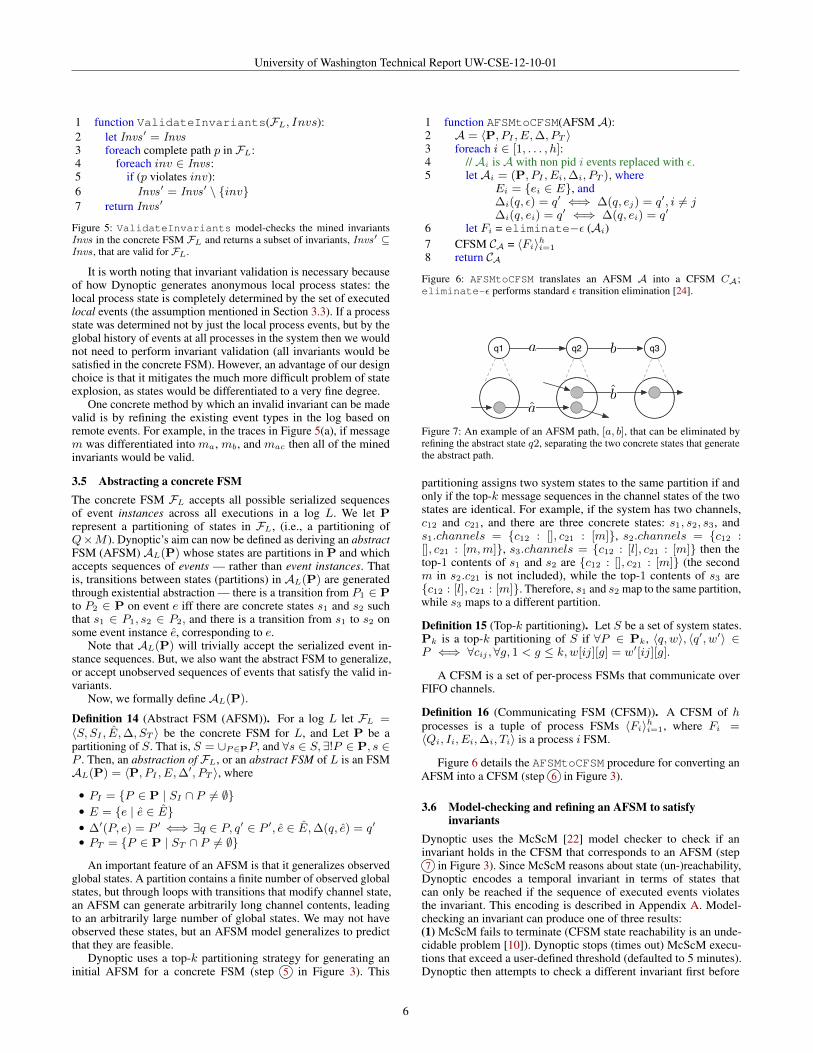
1 function ValidateInvariants(FL, Invs):2 let Invs ′ = Invs3 foreach complete path p in FL:4 foreach inv ∈ Invs:5 if (p violates inv):6 Invs ′ = Invs ′ \ {inv}7 return Invs ′
Figure 5: ValidateInvariants model-checks the mined invariantsInvs in the concrete FSM FL and returns a subset of invariants, Invs′ ⊆Invs , that are valid for FL.
It is worth noting that invariant validation is necessary becauseof how Dynoptic generates anonymous local process states: thelocal process state is completely determined by the set of executedlocal events (the assumption mentioned in Section 3.3). If a processstate was determined not by just the local process events, but by theglobal history of events at all processes in the system then we wouldnot need to perform invariant validation (all invariants would besatisfied in the concrete FSM). However, an advantage of our designchoice is that it mitigates the much more difficult problem of stateexplosion, as states would be differentiated to a very fine degree.
One concrete method by which an invalid invariant can be madevalid is by refining the existing event types in the log based onremote events. For example, in the traces in Figure 5(a), if messagem was differentiated into ma, mb, and mac then all of the minedinvariants would be valid.
3.5 Abstracting a concrete FSMThe concrete FSM FL accepts all possible serialized sequencesof event instances across all executions in a log L. We let Prepresent a partitioning of states in FL, (i.e., a partitioning ofQ×M ). Dynoptic’s aim can now be defined as deriving an abstractFSM (AFSM) AL(P) whose states are partitions in P and whichaccepts sequences of events — rather than event instances. Thatis, transitions between states (partitions) in AL(P) are generatedthrough existential abstraction — there is a transition from P1 ∈ Pto P2 ∈ P on event e iff there are concrete states s1 and s2 suchthat s1 ∈ P1, s2 ∈ P2, and there is a transition from s1 to s2 onsome event instance e, corresponding to e.
Note that AL(P) will trivially accept the serialized event in-stance sequences. But, we also want the abstract FSM to generalize,or accept unobserved sequences of events that satisfy the valid in-variants.
Now, we formally define AL(P).
Definition 14 (Abstract FSM (AFSM)). For a log L let FL =〈S, SI , E,∆, ST 〉 be the concrete FSM for L, and Let P be apartitioning of S. That is, S = ∪P∈PP, and ∀s ∈ S,∃!P ∈ P, s ∈P . Then, an abstraction of FL, or an abstract FSM of L is an FSMAL(P) = 〈P, PI , E,∆
′, PT 〉, where
• PI = {P ∈ P | SI ∩ P 6= ∅}• E = {e | e ∈ E}• ∆′(P, e) = P ′ ⇐⇒ ∃q ∈ P, q′ ∈ P ′, e ∈ E,∆(q, e) = q′
• PT = {P ∈ P | ST ∩ P 6= ∅}
An important feature of an AFSM is that it generalizes observedglobal states. A partition contains a finite number of observed globalstates, but through loops with transitions that modify channel state,an AFSM can generate arbitrarily long channel contents, leadingto an arbitrarily large number of global states. We may not haveobserved these states, but an AFSM model generalizes to predictthat they are feasible.
Dynoptic uses a top-k partitioning strategy for generating aninitial AFSM for a concrete FSM (step 5 in Figure 3). This
1 function AFSMtoCFSM(AFSM A):2 A = 〈P, PI , E,∆, PT 〉3 foreach i ∈ [1, . . . , h]:4 // Ai is A with non pid i events replaced with ε.5 let Ai = (P, PI , Ei,∆i, PT ), where
Ei = {ei ∈ E}, and∆i(q, ε) = q′ ⇐⇒ ∆(q, ej) = q′, i 6= j∆i(q, ei) = q′ ⇐⇒ ∆(q, ei) = q′
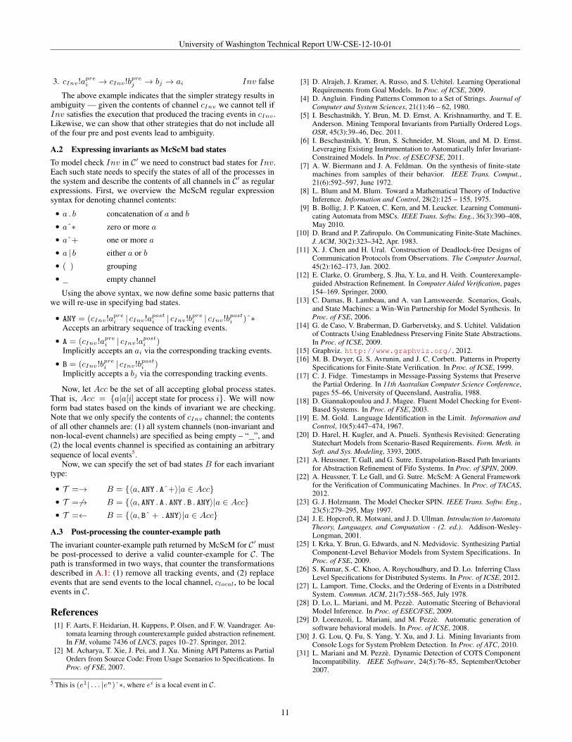
6 let Fi = eliminate−ε (Ai)7 CFSM CA = 〈Fi〉hi=1
8 return CAFigure 6: AFSMtoCFSM translates an AFSM A into a CFSM CA;eliminate-ε performs standard ε transition elimination [24].
q1 q2 q3a b
ba
Figure 7: An example of an AFSM path, [a, b], that can be eliminated byrefining the abstract state q2, separating the two concrete states that generatethe abstract path.
partitioning assigns two system states to the same partition if andonly if the top-k message sequences in the channel states of the twostates are identical. For example, if the system has two channels,c12 and c21, and there are three concrete states: s1, s2, s3, ands1.channels = {c12 : [], c21 : [m]}, s2.channels = {c12 :[], c21 : [m,m]}, s3.channels = {c12 : [l], c21 : [m]} then thetop-1 contents of s1 and s2 are {c12 : [], c21 : [m]} (the secondm in s2.c21 is not included), while the top-1 contents of s3 are{c12 : [l], c21 : [m]}. Therefore, s1 and s2 map to the same partition,while s3 maps to a different partition.
Definition 15 (Top-k partitioning). Let S be a set of system states.Pk is a top-k partitioning of S if ∀P ∈ Pk, 〈q, w〉, 〈q′, w′〉 ∈P ⇐⇒ ∀cij , ∀g, 1 < g ≤ k,w[ij][g] = w′[ij][g].
A CFSM is a set of per-process FSMs that communicate overFIFO channels.
Definition 16 (Communicating FSM (CFSM)). A CFSM of hprocesses is a tuple of process FSMs 〈Fi〉hi=1, where Fi =〈Qi, Ii, Ei,∆i, Ti〉 is a process i FSM.
Figure 6 details the AFSMtoCFSM procedure for converting anAFSM into a CFSM (step 6 in Figure 3).
3.6 Model-checking and refining an AFSM to satisfyinvariants
Dynoptic uses the McScM [22] model checker to check if aninvariant holds in the CFSM that corresponds to an AFSM (step7 in Figure 3). Since McScM reasons about state (un-)reachability,
Dynoptic encodes a temporal invariant in terms of states thatcan only be reached if the sequence of executed events violatesthe invariant. This encoding is described in Appendix A. Model-checking an invariant can produce one of three results:(1) McScM fails to terminate (CFSM state reachability is an unde-cidable problem [10]). Dynoptic stops (times out) McScM execu-tions that exceed a user-defined threshold (defaulted to 5 minutes).Dynoptic then attempts to check a different invariant first before
6

University of Washington Technical Report UW-CSE-12-10-01
coming back to the invariant that timed out 3. If checking each ofthe remaining invariants times out, Dynoptic gives up.(2) The invariant holds in the model. Dynoptic either moves on to thenext invariant, or terminates and outputs the model if all invariantshave been satisfied.(3) The invariant does not hold and McScM finds and reports acounter-example CFSM execution. A CFSM execution is a sequenceof events that abides by CFSM semantics (e.g., a process can onlyreceive a message if that message is at the top of the channel),and the events sequence leads the system into state in which eachof the processes is in a terminal state, and all channels are empty.A counter-example CFSM execution is a sequence of events thatviolates the invariant. In this case, Dynoptic uses counter-exampleguided abstraction refinement (CEGAR) approach [12] to refine theAFSM to eliminate the counter-example. The rest of this sectiondetails this refinement.
Dynoptic uses partition refinement to eliminate a counter-example for an invariant — once all invariant counter-exampleshave been eliminated, the model satisfies the invariant. Figure 7illustrates how the concrete states from the log may generate acounter-example trace in the AFSM. The McScM invariant counter-example is a CFSM execution, but refinement must occur in theAFSM. So, Dynoptic maps the McScM-generated CFSM counter-example into an AFSM counter-example. Figure 8 describes thistranslation.
Definition 17 (Invariant counter-example). Let L be a log, letInv be a valid invariant for L, and let A be an AFSM for L.Then, a CFSM counter-example to Inv in CFSM CA (derived withAFSMtoCFSM in Figure 6) is a sequence of events p that doesnot satisfy Inv and is an execution of CA. The AFSM counter-example corresponding to p is the sequence of sets, S, where eachset contains paths in A. The sequence S is derived using S =TranslatePath(p, CA) (Figure 8).
Note that the AFSM counter-example is a sequence of sets ofAFSM paths, one for each process in the system. This is becausethe process-specific events subsequence of a CFSM execution maybe generated by multiple paths in the AFSM (due to the CFSMconstruction based on ε-transitions in Figure 6).
Once the AFSM counter-example is generated, Dynoptic usespartition refinement (Refine in Figure 9) to eliminate the CFSMcounter-example by transforming the AFSM into a more concrete (orless abstract) AFSM. Refinement corresponds to step 8 in Figure 3.For each AFSM path, Refine identifies the set of partitions thatstitch concrete observations, as in partition q2 in Figure 7. It thenrefines all partitions in a set that is smallest across all processes andreturns the refined AFSM.
A refined AFSM is more concrete because the states of therefined AFSM contain fewer system states observed in the log, andtherefore the AFSM is closer to the concrete FSM.
Definition 18 (AFSM Refinement). An AFSM AL(P′) is a refine-ment of AFSM AL(P) if ∀P ′ ∈ P′, ∃P ∈ P, P ′ ⊆ P .
The complete Dynoptic algorithm is listed in Figure 10. Next,we prove a few key properties of the Dynoptic process.
4. Formal analysisWe begin with an observation: the concrete FSM satisfies all valid in-variants. This is true by construction in ValidateInvariantsin Figure 5.
3 After refining the model to satisfy an invariant, a previously difficult-to-check invariant may become trivial to model-check
1 function TranslatePath(p, CA):2 // p is a complete events path in CFSM CA3 let AFSM A = 〈P, PI , E,∆, PT 〉4 foreach i ∈ [1, . . . , h]:5 let Si = {s | s an events path in A from P1 to Pk,
π(s, Ei) = π(p,Ei), P1 ∈ PI ,∃〈q, w〉 ∈ Pk, q[i] terminal, and
∀j, w[ji] = ε}6 return [S1, . . . , Sh]
Figure 8: TranslatePath translates an events path p in a CFSM CA intoS, a sequence of sets of paths inA. Each set in S maps to one event in p.
1 function Refine(A, S, L):2 // S is derived via TranslatePath3 let AFSM A = (P, PI , E,∆, PT )4 let Stitchmin = ∅5 foreach i ∈ [1, . . . , h]:6 foreach s ∈ S[i]:7 let Ps = state sequence for s in A8 // Derive stitching states, e.g., q2 in Fig. 79 let Stitchs = {p | p a stitching state in Ps}
10 if Stitchs = ∅:11 next i12 // Partitions set shared by paths that generate s13 Stitchi = ∩s∈S[i]Stitchs
14 // Stitchmin is the min size set over all Stitchi
15 if Stitchmin = ∅ or |Stitchi| < |Stitchmin|:16 Stitchmin = Stitchi
17 let P′ = P with all partitions in Stitchmin refined18 // Derive P ′I ,∆
′, and P ′T from P′ as in Def. 18.19 let AFSM A′ = 〈P′, P ′I , E,∆′, P ′T 〉20 return A′
Figure 9: Refine removes an invariant counter-example from an AFSM byrefining the set of process paths in S that require the fewest refinements.
1 function Dynoptic (Log L, k):2 let Invs =
ValidateInvariants(MineInvariants(L))3 let FL = Concrete FSM for L4 let A = AFSM for FL with partitioning Pk
5 let CA = AFSMtoCFSM(A)6 foreach Inv ∈ Invs:7 while (CA violates Inv): // Call to model checker.8 let p = counter-example path for Inv in CA9 let S = TranslatePath(p, CA)
10 A = Refine(A, S, L)11 CA = AFSMtoCFSM(A)12 return CA
Figure 10: The complete Dynoptic algorithm.
Observation 1 (Concrete FSM satisfies valid invariants). Let L bea log, and let Invs be the set of invariants that are valid in FL. Then,∀Inv ∈ Invs, t ∈ Lang(FL), t satisfies Inv.
A key property of the Refine procedure in Figure 9 is that iteliminates the counter-example path from the CFSM correspondingto the current AFSM. We prove this next.
Theorem 1 (Refinement eliminates counter-examples). Let pbe a CFSM counter-example path for Inv in CA and let S =TranslatePath(p, CA), and let A′ = Refine(A, S, L). Then,
7

University of Washington Technical Report UW-CSE-12-10-01
p is not a counter-example to Inv in CA′ . That is, p is not a validexecution of CA′ .
Proof of Theorem 1. We prove this by contradiction. Assume thatp is a sequence of events that is a valid execution of CA′ and that pviolates Inv. Let Stitchmin = Stitchi for some i in the executionof Refine(A, S, L) procedure in Fig. 9. Also, let CA′ = 〈Fi〉hi=1.
For p to be a valid execution in CA′ , the sub-sequence of processi events pi, pi = π(p,Ei), must be a valid execution in Fi. TheProcedure AFSMtoCFSM in Fig. 6 constructs Fi to accept pi iffthere is a complete path s in A′, such that pi = π(s, Ei). However,any such smust also be in Stitchi. Therefore, after refining Stitchi,s can no longer be a valid path in A′. Contradiction.
Now, we prove that the Dynoptic procedure in Figure 10returns a CFSM model that satisfies all of the valid invariants.
Theorem 2 (True invariant satisfiability). For a given log L,Dynoptic produces a CFSM model that satisfies all of theevent invariants that are valid in FL.
Proof of Theorem 2. For a log L with a total of n event instances,Dynoptic can refine the initial abstract FSM for L, AL(Pk), atmost n times. This is because after n refinements, each partition inthe abstract FSM would map to exactly one concrete state, and asingleton partition cannot be refined further.
Let A be the abstract FSM after n refinements of AL(Pk).Because A maps each event instance to a unique partition, it isindistinguishable from the concrete FSM it abstracts, FL. Therefore,Lang(A) = Lang(FL). By Observation 1, FL satisfies all validinvariants, therefore so does A.
Since Dynoptic does not terminate until all the valid invariantsare satisfied in the abstract FSM, it either returns A after n refine-ments, or it returns a smaller (and more abstract) A′. In both cases,the returned AFSM satisfies all of the valid invariants.
5. Experimental evaluationThe Dynoptic prototype is implemented in Java, uses the McScMmodel checker as a black box, and leverages graphviz [15] formodel visualization. We evaluated Dynoptic on logs producedby a simulator of the alternating bit protocol and by two realsystems — the TCP stack of the Mac OS X operating system;and Voldemort [40], a large open source project that implementsa distributed hash tableand is used in data centers at companieslike LinkedIn. In this paper, we do not evaluate whether Dynoptic-generated models are intuitive or useful to developers. We plan todo a user study evaluation of Dynoptic as part of our future work.
5.1 Alternating bit protocolWe considered traces from a simulator of the alternating bit pro-tocol described in Section 2. We derived a diverse set of tracesby varying message delays to produce different message interleav-ings. Dynoptic mined a total of 66 valid invariants, and Figure 1shows the Dynoptic-derived model. This experiment was a san-ity check to verify that Dynoptic performed as expected on thiswell-understood protocol, when faced with delays and concurrency-induced non-determinism in interleavings. The model Dynopticderived is identical to the true model of the alternating bit protocol.
5.2 TCPThe TCP protocol uses a three-way opening handshake to establisha bi-directional communication channel between two end-points. Ittears down and cleans up the connection using a four-way closing
handshake. The TCP state machine is complicated by the fact thatpacket delays and packet losses cause the end-points to timeout andre-transmit certain packets, which may in turn induce new messages.Our initial goal was to model common-case TCP behavior, so wedid not explore these protocol corner cases.
We used a combination of netcat and dummynet [35] to generateand control TCP packet flow. We captured packets using tcpdumpand then annotated the log to include vector timestamps. Theresulting traces were fed into Dynoptic, which was used to modeljust the opening and closing TCP handshakes.
For the captured TCP log, Dynoptic identified 149 valid invari-ants, some of which are not true of the complete protocol (e.g.,because the input traces did not contain certain packet retrans-missions). The Dynoptic-derived CFSM model is shown in Fig-ure 11. The shaded states s4 and c4 represent the server and clientconnection-established states, which is attained when thetwo end-points have successfully set up the bi-directional channel.Transitions up to these two states model the opening handshake,while transitions after these states model the closing handshake. Theclosing handshake is split into a server-initiated tear-down sequence(middle row of states) and a client-initiated tear-down (bottom-mostrow of states).
The derived model is accurate except for the self-loop on states4 in Figure 11(a). This loop appears because s4 merges theconnection-established state with the state after the serverhas initiated the closing handshake. This loop appears to contradictthe SC!fin 6→ SC!fin invariant, which is mined by Dynopticfor the input traces and is valid. However, the model checkeronly considers counter-examples that terminate. Note that if theloop in the model is traversed twice then the client will not beable to consume both server fin packet copies and will enter anunspecified reception error state and therefore not terminate. Suchunspecified reception states are typically undesirable, as they can beconfusing. The McScM model checker can be used to detect thesestates and further refinement will eliminate them. Implementing thiselimination remains as part of future work.
5.3 Voldemort distributed hash tableVoldemort implements a distributed hash table with a client APIthat has two main methods: put(k,v) — associate the value vwith the key k, and get(k) — retrieve the current value associatedwith the key k. Voldemort is a distributed system as it providesscalability by partitioning the key space across multiple machinesand achieves fault tolerance by replicating keys and values acrossmultiple machines.
The Voldemort project has an extensive test suite, which weleverage to generate a log of replication messages in a system withone client and two replicas. We logged messages generated by clientcalls to the synchronized versions of put and get and captured justthe messages between the client and the two replicas. (The replicasalso communicate with each other to maintain key availability, butwe excluded this communication from the log.)
Dynoptic mined 112 valid invariants and generated the modelin Figure 12. This model contains a client FSM and two replicaFSMs. As expected, the replica FSMs are identical. SynchronizedVoldemort operations are serialized in a specific order, so the flowof messages for put as well as for get is identical — the clientfirst executes the operation at replica 1 and then at replica 2.
The model is accurate and provides a high-level overview ofhow replication messages flow in the system. However, the model isalso abstract and is missing important details, such as what happenswhen replicas fail. An advantage of the Dynoptic technique is thata developer can focus on aspects of behavior that are important tothem and ignore irrelevant details. We plan to study other aspects ofthe Voldemort system with Dynoptic in our future work.
8

University of Washington Technical Report UW-CSE-12-10-01
s1 s2SC!syn-ack s3CS?ack s4SC!ackCS?syn
(a) TCP server (b) TCP client
s0
SC!fin
s5s6 SC!ack
s9
CS?ack
CS?fins10 SC!ack
s7 CS?fin
s11 CS?ack
s8 SC!ack
s12 SC!fin
CS?ack
c1 c2SC?syn-ack c3CS!ack c4SC?ackCS!sync0
c5c6 CS!ack
c10
SC?fin
CS!finc11 SC?ack
c7 SC?ack
c12 CS!ack
c9 CS!fin
c13 SC?fin
CS!ack
c8SC?ack
SC
CS
Figure 11: The inferred (a) TCP server, and (b) TCP client state machines. The server communicates with the client over the SC channel, and the clientcommunicates with the server over the CS channel. Shaded states represent the connection-established states.
(a) Voldemort Replica 1 (b) Voldemort client
c1
c2
R1-C?put-re
c3 C-R2!put
R2-C?put-re
C-R1!putc0R1-C
C-R1
c4
c5
R1-C?get-re
c6C-R2!get
R2-C?get-re
C-R1!get
r1r0r2
R1-C!get-re
C-R1?get C-R1?put
R1-C!put-re
(c) Voldemort Replica 2
s1s0s2
R2-C!get-re
C-R2?get C-R2?put
R2-C!put-re
R2-C
C-R2
Figure 12: The inferred star-topology within a three node Voldemort cluster with (a,c) the Voldemort replica models, and (b) the Voldemort client model.
6. Related workCFSMs inferred from executions can demonstrate certain properties,such as absence of deadlocks and unspecified receptions [11, 39].This prior work is theoretical, and while such properties are impor-tant in theory, in practice, we found that they are not necessary togenerate models that provide insight into system implementation.Bollig et al.have also explored the problem of inferring a CFSMfrom message sequence charts [9]. However, these charts must bemanually labeled as positive or negative examples of system behav-ior. In contrast, Dynoptic relies on mined invariants and automatesthe inference process. Recent work by Kumar et al.considers theproblem of inferring class level specifications of distributed systems,in the form of symbolic message sequence charts [26]. This workcan be used by Dynoptic to abstract process FSMs that are identical(e.g., the replica models in Figure 12(a,c)).
More broadly, systems logs have been previously used to detectanomalies [30, 43], performance bugs [36], and to mine temporalsystem properties [44]. In contrast, Dynoptic focuses on extracting amodel that can aid understanding of more general system behavior,particularly focusing on concurrency.
Dynoptic’s goal is to find a short sequence of refinements toproduce a small (abstract) AFSM that satisfies all of the validinvariants. This problem is NP-hard [12], and Dynoptic is designedto approximate the solution. For logs of serial systems (totallyordered logs), the problem of automata inference from positiveexamples of executions is computable [8], but NP-complete [4, 19],and the FSA cannot be approximated by any polynomial-timealgorithm [33]. Unlike Dynoptic, prior work on model inferencefrom totally ordered logs either excluded concurrency altogether orcaptured a particular interleaving of concurrent events [2, 6, 7, 7,29, 29, 31, 31, 34, 34]. Meanwhile, Dynoptic captures concurrencyas a partial order, which we believe is crucial to helping developersunderstand a concurrent system’s behavior.
The closest total-order log work to Dynoptic is Synoptic [6]and Tomte [1], both of which leverage CEGAR [12]. Synopticmines temporal invariants and infers FSM models from a log ofsequential executions while Tomte infers scalarset Mealy machines.In contrast to both of these tools, Dynoptic accounts for richer kinds
of invariants, deals with a richer model type, and provides insightinto partially ordered logs.
System models can also be inferred from developer-writtenspecifications [3, 13, 14, 18, 20, 25, 38, 41]. Compared to Dynoptic,these techniques require significantly more manual effort from thedeveloper and may not be suitable for legacy systems.
Dynoptic relies on the McScM model checker [21, 22] for check-ing the validity of invariants in a CFSM model. A key property ofMcScM is that unlike most CFSM verification tools, like SPIN [23],McScM verifies models with no apriori bound on channel size.However, McScM is not guaranteed to terminate. To make modelchecking more tractable (and faster) we plan to extend Dynopticto support model checkers that verify CFSM models with boundedchannel lengths.
. . .
7. DiscussionThe vector timestamps Dynoptic requires may adversely affect thesystem’s performance and increase its implementation complexity.However, in certain cases, this requirement may be relaxed andvector timestamps may be inferred from real-time timestamps andmessage identifiers, such as request ids.
CFSM models (Def 16) may contain two kinds of errorstates [10] — unspecified reception and deadlock — neither ofwhich can be eliminated directly by Dynoptic’s model construction.Unspecified reception occurs when a process enters a state with amessage m at the head of its channel, but has no reachable futurestate that has a transition to receive m. A deadlocked system stateoccurs when no process can send a message and at least one processcannot reach a terminating state. Currently, Dynoptic does not checkif these error states are reachable in the final model. It is possibleto extend Dynoptic with such a check, for example, by using theMcScM model checker, but the check would be expensive.
Dynoptic mines three types of invariants and ensures that thefinal model satisfies the valid invariants subset. While we foundthese invariant types to be sufficient to infer interesting modelsin practice, more extensive invariants can lead to more expressivemodels. For example, a developer might know of a property that
9

University of Washington Technical Report UW-CSE-12-10-01
the system must satisfy and might want Dynoptic to require thatthe final model preserves it if this property is true of the input log.In this case, the developer may extend Dynoptic to support a user-defined LTL invariant by (1) implementing a miner to mine invariantinstances of this type from the log, and (2) sub-classing and updatinga basic template that encodes invariants for model checking with theMcScM model checker.
Dynoptic works for system traces that satisfy certain communi-cation constraints (Def. 6). For example, Dynoptic cannot modelunclean termination and assumes that each execution terminateswith empty channels. However, in practice, system logs may notsatisfy these constraints. For example, it might not be possible toacquiesce a production system to process all outstanding messages.In our future work we will extend Dynoptic to handle terminal stateswith non-empty channels. One way to do this is to introduce a termi-nal state qti for each process i, and append synthetic receive events toeach trace to receive all outstanding messages while remaining in theqti state. This drains non-empty channels and converts incompatibletraces into ones that Dynoptic can already process.
8. ContributionsSystems with concurrent components are hard to implement, debug,and verify. To help with these tasks, we developed Dynoptic, anautomated tool that uses a partially ordered log of events to infera concise and precise communicating finite state machine modelof the system. Dynoptic’s precision comes from its use of minedtemporal properties that relate events in the log.
We have evaluated Dynoptic in two ways. First, we formallydefined the Dynoptic models and the model derivation process andproved that (1) the Dynoptic process eliminates property counter-examples produced by model-checking, and (2) the final modelsatisfies the subset of properties that are valid. Second, we imple-mented Dynoptic and ran it on logs produced by three distributedsystems/protocols — the alternating bit protocol, TCP, and Volde-mort, a distributed storage system.
By automatically mining a system model from logs Dynoptichas the potential to ease system understanding, debugging, andmaintenance tasks. In our future work, we will empirically verifythat Dynoptic helps developers with these tasks. Thus far, the initialmodels derived in this paper show significant promise.
A. Checking invariants with McScMModel checking an event invariant (Section 3.2) in a CFSM (Sec-tion 3.5) is a two step process. First, the CFSM must be augmentedwith synthetic “tracking” transitions that record when an event typementioned by the invariant is executed by the model checker. Sec-ond, the negation of the invariant must be encoded as a set of “badstates” of the CFSM. If the model checker finds an execution thatcan reach one of these states, it will emit the path, which is exactlythe counter-example path for the invariant. We now describe both ofthese steps in more detail.
A.1 Preparing a CFSM for model checkingConsider an event invariant Inv, such that Inv = aiT bj , withT ∈ {→, 6→,←}. And, let C be a CFSM in which we want tocheck if Inv holds.
We modify C to produce a new CFSM model, C′, which willbe used as input to the McScM model checker. We tranform C intoC′ in two ways — we convert local events into send events on asynthetic channel, and we add synthetic “tracking events” to trackthe execution of ai and bj event types.
Handling local events. The McScM model checker does notmodel local events (it only supports message send and receiveevents). We cannot omit local events from C′, as we need to be
q q'
q'' q''' aiq q'cInv!aprei cInv!apost
i
ai
Figure 13: Transforming an edge in a CFSM to track ai.
able to unambiguously map an McScM counter-example path in C′to a path in C. We therefore add a synthetic “local events” channel,clocal, and allow all processes to send messages on clocal. Thischannel is write-only — processes never receive on clocal. Finally,each process local event type, ei, in C is translated into the eventtype clocal!ei in C′. That is, we replace transitions of the form∆i(q, ei) = q′ with ∆i(q, clocal!ei) = q′.
Tracking events necessary for checking Inv. Given a CFSMand a set of “bad states”, the McScM model checker checks if thereis an execution of the input CFSM that causes it to reach one ofthe bad states. A bad state is a kind of a system state (introduced inSection 3.3) — it is a pair of global process state and global channelstate. In McScM the global channel state is expressed as regularexpressions over channel contents4.
To check Inv with McScM, we therefore need to generate a setof system states of C′, each of which encodes a violation of Inv.To generate this encoding for Inv = aiT bj we need to track whenai or bj occur. We do this with “tracking events”, which track theoccurrence of ai and bj as send events to a synthetic Inv-specificchannel, cInv . This channel is used exclusively for checking Inv.As with the synthetic local events channel, all processes can sendon cInv , and no process ever receives from this channel. Figure 13illustrates this tracking. More formally, if ∆i is the process i FSMtransition function in C, then we track ai and bj event types asfollows:
• Replace transitions of the form ∆i(q, ai) = q′ with:
∆i(q, cInv!aprei ) = q′′
∆i(q′′, ai) = q′′′
∆i(q′′′, cInv!aposti ) = q′
Where, q′′, q′′′ are synthetic states with just the transitions above,and cInv!aprei and cInv!aposti are synthetic event types thatmaintain a record of when ai occurs as messages in cInv .• Similarly, to keep track of bj , replace ∆j(p, bj) = p′ with:
∆j(p, cInv!bprej ) = p′′
∆j(p′′, bj) = p′′′
∆j(p′′′, cInv!bpostj ) = p′
Note that both of the transformations retain the event ai or bj .This is necessary as we want C′ to have identical behavior to C.
To see why we need to augment both ai and bj with a pre anda post event, consider other strategies, with less overhead (fewersynthetic events). For example, assume that Inv = ai → bjand we repaced transitions of the form ∆i(q, ai) = q′ with∆i(q, cInv!aprei ) = q′′ and ∆i(q
′′, ai) = q′; and we replacedtransitions of the form ∆j(p, bj) = p′ with ∆j(p, cInv!bprej ) = p′′
and ∆j(p′′, bj) = p′.
Then, consider the following contents of cInv: [aprei , bprej ].These two tracking events imply one of three executions:
1. cInv!aprei → ai → cInv!bprej → bj Inv true
2. cInv!aprei → cInv!bprej → ai → bj Inv true
4 Therefore, an McScM bad state is in fact a set of system states, as definedin Section 3.3.
10
University of Washington Technical Report UW-CSE-12-10-01
3. cInv!aprei → cInv!bprej → bj → ai Inv false
The above example indicates that the simpler strategy results inambiguity — given the contents of channel cInv we cannot tell ifInv satisfies the execution that produced the tracing events in cInv .Likewise, we can show that other strategies that do not include allof the four pre and post events lead to ambiguity.
A.2 Expressing invariants as McScM bad statesTo model check Inv in C′ we need to construct bad states for Inv.Each such state needs to specify the states of all of the processes inthe system and describe the contents of all channels in C′ as regularexpressions. First, we overview the McScM regular expressionsyntax for denoting channel contents:
• a . b concatenation of a and b• aˆ∗ zero or more a• aˆ+ one or more a• a | b either a or b• ( ) grouping• empty channel
Using the above syntax, we now define some basic patterns thatwe will re-use in specifying bad states.
• ANY = (cInv!aprei | cInv!aposti | cInv!bprei | cInv!bposti )ˆ∗Accepts an arbitrary sequence of tracking events.• A = (cInv!aprei | cInv!aposti )
Implicitly accepts an ai via the corresponding tracking events.• B = (cInv!bprei | cInv!bposti )
Implicitly accepts a bj via the corresponding tracking events.
Now, let Acc be the set of all accepting global process states.That is, Acc = {a|a[i] accept state for process i}. We will nowform bad states based on the kinds of invariant we are checking.Note that we only specify the contents of cInv channel; the contentsof all other channels are: (1) all system channels (non-invariant andnon-local-event channels) are specified as being empty – “ ”, and(2) the local events channel is specified as containing an arbitrarysequence of local events5.
Now, we can specify the set of bad states B for each invarianttype:
• T =→ B = {〈a, ANY . Aˆ+〉|a ∈ Acc}• T = 6→ B = {〈a, ANY . A . ANY . B . ANY〉|a ∈ Acc}• T =← B = {〈a, Bˆ + . ANY〉|a ∈ Acc}
A.3 Post-processing the counter-example pathThe invariant counter-example path returned by McScM for C′ mustbe post-processed to derive a valid counter-example for C. Thepath is transformed in two ways, that counter the transformationsdescribed in A.1: (1) remove all tracking events, and (2) replaceevents that are send events to the local channel, clocal, to be localevents in C.
References[1] F. Aarts, F. Heidarian, H. Kuppens, P. Olsen, and F. W. Vaandrager. Au-
tomata learning through counterexample guided abstraction refinement.In FM, volume 7436 of LNCS, pages 10–27. Springer, 2012.
[2] M. Acharya, T. Xie, J. Pei, and J. Xu. Mining API Patterns as PartialOrders from Source Code: From Usage Scenarios to Specifications. InProc. of FSE, 2007.
5 This is (e1| . . . |en)ˆ∗, where ei is a local event in C.
[3] D. Alrajeh, J. Kramer, A. Russo, and S. Uchitel. Learning OperationalRequirements from Goal Models. In Proc. of ICSE, 2009.
[4] D. Angluin. Finding Patterns Common to a Set of Strings. Journal ofComputer and System Sciences, 21(1):46 – 62, 1980.
[5] I. Beschastnikh, Y. Brun, M. D. Ernst, A. Krishnamurthy, and T. E.Anderson. Mining Temporal Invariants from Partially Ordered Logs.OSR, 45(3):39–46, Dec. 2011.
[6] I. Beschastnikh, Y. Brun, S. Schneider, M. Sloan, and M. D. Ernst.Leveraging Existing Instrumentation to Automatically Infer Invariant-Constrained Models. In Proc. of ESEC/FSE, 2011.
[7] A. W. Biermann and J. A. Feldman. On the synthesis of finite-statemachines from samples of their behavior. IEEE Trans. Comput.,21(6):592–597, June 1972.
[8] L. Blum and M. Blum. Toward a Mathematical Theory of InductiveInference. Information and Control, 28(2):125 – 155, 1975.
[9] B. Bollig, J. P. Katoen, C. Kern, and M. Leucker. Learning Communi-cating Automata from MSCs. IEEE Trans. Softw. Eng., 36(3):390–408,May 2010.
[10] D. Brand and P. Zafiropulo. On Communicating Finite-State Machines.J. ACM, 30(2):323–342, Apr. 1983.
[11] X. J. Chen and H. Ural. Construction of Deadlock-free Designs ofCommunication Protocols from Observations. The Computer Journal,45(2):162–173, Jan. 2002.
[12] E. Clarke, O. Grumberg, S. Jha, Y. Lu, and H. Veith. Counterexample-guided Abstraction Refinement. In Computer Aided Verification, pages154–169. Springer, 2000.
[13] C. Damas, B. Lambeau, and A. van Lamsweerde. Scenarios, Goals,and State Machines: a Win-Win Partnership for Model Synthesis. InProc. of FSE, 2006.
[14] G. de Caso, V. Braberman, D. Garbervetsky, and S. Uchitel. Validationof Contracts Using Enabledness Preserving Finite State Abstractions.In Proc. of ICSE, 2009.
[15] Graphviz. http://www.graphviz.org/, 2012.[16] M. B. Dwyer, G. S. Avrunin, and J. C. Corbett. Patterns in Property
Specifications for Finite-State Verification. In Proc. of ICSE, 1999.[17] C. J. Fidge. Timestamps in Message-Passing Systems that Preserve
the Partial Ordering. In 11th Australian Computer Science Conference,pages 55–66, University of Queensland, Australia, 1988.
[18] D. Giannakopoulou and J. Magee. Fluent Model Checking for Event-Based Systems. In Proc. of FSE, 2003.
[19] E. M. Gold. Language Identification in the Limit. Information andControl, 10(5):447–474, 1967.
[20] D. Harel, H. Kugler, and A. Pnueli. Synthesis Revisited: GeneratingStatechart Models from Scenario-Based Requirements. Form. Meth. inSoft. and Sys. Modeling, 3393, 2005.
[21] A. Heussner, T. Gall, and G. Sutre. Extrapolation-Based Path Invariantsfor Abstraction Refinement of Fifo Systems. In Proc. of SPIN, 2009.
[22] A. Heussner, T. Le Gall, and G. Sutre. McScM: A General Frameworkfor the Verification of Communicating Machines. In Proc. of TACAS,2012.
[23] G. J. Holzmann. The Model Checker SPIN. IEEE Trans. Softw. Eng.,23(5):279–295, May 1997.
[24] J. E. Hopcroft, R. Motwani, and J. D. Ullman. Introduction to AutomataTheory, Languages, and Computation - (2. ed.). Addison-Wesley-Longman, 2001.
[25] I. Krka, Y. Brun, G. Edwards, and N. Medvidovic. Synthesizing PartialComponent-Level Behavior Models from System Specifications. InProc. of FSE, 2009.
[26] S. Kumar, S.-C. Khoo, A. Roychoudhury, and D. Lo. Inferring ClassLevel Specifications for Distributed Systems. In Proc. of ICSE, 2012.
[27] L. Lamport. Time, Clocks, and the Ordering of Events in a DistributedSystem. Commun. ACM, 21(7):558–565, July 1978.
[28] D. Lo, L. Mariani, and M. Pezze. Automatic Steering of BehavioralModel Inference. In Proc. of ESEC/FSE, 2009.
[29] D. Lorenzoli, L. Mariani, and M. Pezze. Automatic generation ofsoftware behavioral models. In Proc. of ICSE, 2008.
[30] J. G. Lou, Q. Fu, S. Yang, Y. Xu, and J. Li. Mining Invariants fromConsole Logs for System Problem Detection. In Proc. of ATC, 2010.
[31] L. Mariani and M. Pezze. Dynamic Detection of COTS ComponentIncompatibility. IEEE Software, 24(5):76–85, September/October2007.
11

University of Washington Technical Report UW-CSE-12-10-01
[32] F. Mattern. Virtual Time and Global States of Distributed Systems. InParallel and Distributed Algorithms, pages 215–226, 1989.
[33] L. Pitt and M. K. Warmuth. The Minimum Consistent DFA ProblemCannot be Approximated Within any Polynomial. J. ACM, 40(1):95–142, 1993.
[34] S. P. Reiss and M. Renieris. Encoding Program Executions. In Proc. ofICSE, 2001.
[35] L. Rizzo. Dummynet: a Simple Approach to the Evaluation of NetworkProtocols. CCR, 27(1):31–41, Jan. 1997.
[36] R. R. Sambasivan, A. X. Zheng, M. D. Rosa, E. Krevat, S. Whitman,M. Stroucken, W. Wang, L. Xu, and G. R. Ganger. DiagnosingPerformance Changes by Comparing Request Fows. In Proc. of NSDI,2011.
[37] G. Tel. Introduction to distributed algorithms. Cambridge UniversityPress, New York, NY, USA, 1994.
[38] S. Uchitel, J. Kramer, and J. Magee. Incremental Elaboration ofScenario-Based Specifications and Behavior Models Using ImpliedScenarios. ACM TOSEM, 13(1), 2004.
[39] H. Ural and H. Yenigun. Towards Design Recovery from Observations,volume 3235, chapter 9, pages 133–149. Springer Berlin Heidelberg,Berlin, Heidelberg, 2004.
[40] Voldemort. http://project-voldemort.com, 2012.[41] J. Whittle and J. Schumann. Generating Statechart Designs From
Scenarios. In Proc. of ICSE, 2000.[42] W. Xu, L. Huang, A. Fox, D. Patterson, and M. Jordan. Experience
mining Google’s production console logs. In Proc. of SLAML, 2010.[43] W. Xu, L. Huang, A. Fox, D. Patterson, and M. I. Jordan. Detecting
Large-Scale System Problems by Mining Console Logs. In Proc. ofSOSP, 2009.
[44] J. Yang, D. Evans, D. Bhardwaj, T. Bhat, and M. Das. Perracotta:Mining Temporal API Rules from Imperfect Traces. In Proc. of ICSE,2006.
12