land

Article

Inferring Missing Climate Data for AgriculturalPlanning Using Bayesian Networks

Leonel Lara-Estrada 1,2,*, Livia Rasche 1, L. Enrique Sucar 3 and Uwe A. Schneider 1 ID

1 Research Unit Suitability and Global Change, Center for Earth System Research and Sustainability,Universität Hamburg, Grindelberg 5, 20144 Hamburg, Germany; livia.rasche@uni-hamburg.de (L.R.);uwe.schneider@uni-hamburg.de (U.A.S.)

2 School of Integrated Climate System Sciences, CLISAP, Grindelberg 5, 20144 Hamburg, Germany3 Instituto Nacional de Astrofísica, Óptica y Electrónica, Luis Enrique Erro # 1, Tonantzintla, 72840 Puebla,

Mexico; esucar@inaoep.mx* Correspondence: Leonel_larae@hotmail.com; Tel.: +49-40-42838-6593

Received: 16 October 2017; Accepted: 5 January 2018; Published: 10 January 2018

Abstract: Climate data availability plays a key role in development processes of policies, services,and planning in the agricultural sector. However, data at the spatial or temporal resolution requiredis often lacking, or certain values are missing. In this work, we propose to use a Bayesian networkapproach to generate data for missing variables. As a case study, we use relative humidity, which isan important indicator of land suitability for coffee production. For the model, we first extractedclimate data for the variables precipitation, maximum and minimum air temperature, wind speed,solar radiation and relative humidity from the surface reanalysis dataset Climate Forecast SystemReanalysis. We then used machine learning algorithms to define the model structure and parametersfrom the relationships of the variables found in the dataset. Precipitation, maximum and minimumair temperature, wind speed, and solar radiation are then used as proxy variables to infer missingvalues for monthly relative humidity and relative humidity for the driest month. For this, we usedboth complete and incomplete initial data. In both scenarios of data availability, the comparison ofestimated and measured values of relative humidity shows a high level of agreement. We concludethat using Bayesian Networks is a practical solution to estimate relative humidity for coffeeagricultural planning.

Keywords: probabilistic modeling; machine learning; modeling climate information; graphical models;proxy climatic variables; land evaluation; Central America; Coffea arabica L.

1. Introduction

Missing data is a major challenge for agricultural planning, reporting and research not onlyat the level of individual farms, but also at regional, national, or international scales. Incompleteinformation leads to misrepresentation and bias, but collecting the missing data can be very costly [1,2].Several procedures have been employed in previous applications to deal with data gaps. For example,the Agricultural Resource Management Survey in the USA uses conditional or national averages withor without outliers [2]. In agricultural research, data gaps have been filled by combining survey andsatellite information [3], spatial interpolations [4], introduction of proxy variables [5], and, in the caseof climate research, by using the regularized EM algorithm for Gaussian data [6], empirical orthogonalfunctions [4], grouping methods of data handling [7], and others.

A scarcity of data, data with a high uncertainty attached or inhomogeneous data from differentsources is especially prevalent in developing countries. While the procedures described above aremostly suitable for dealing with the problem, their practical implementation in developing countriesis often difficult due to a lack of qualified personnel and financial shortfalls [8–10]. For example,

Land 2018, 7, 4; doi:10.3390/land7010004 www.mdpi.com/journal/land

Land 2018, 7, 4 2 of 13

in several Central American countries, the reconstruction of climate variables using interpolationmethods was only possible with external funding from the World Bank [10]. To overcome these hurdles,we propose to use a Bayesian network (BN), which is a mathematical model that graphically representsconditional probabilistic dependencies between variables. BNs can deal with uncertainty, missing data,missing (hidden) variables and small datasets; it is possible to learn the graphical structure and theparameters of the model from data, literature, expert knowledge or a combination of all [11–14].Another practical advantage of using BN is the availability of free software [15,16].

In a BN approach, data can be generated for variables with missing values while maintaininga consistent relationship with other variables in the same dataset [17]. It also allows the user toincorporate the uncertainty surrounding input data by entering a range or distribution of possiblevalues or by using the prior information parameterized in the model when no information is available.Instead of a single, certain value, the output is then the most probable value of the variable of interestwith the uncertainty attached [11,14,18]. The Bayesian ability to handle uncertainty in the modelingprocess is advantageous, considering that uncertain and missing data are common in real-worldsituations [19], especially when dealing with climate variables and when working in regions withoutgood data coverage [10,20,21].

There are several options in BNs for dealing with missing data: removing the registers withmissing values; using mode values in place of the missing values or estimating the missing values basedon the values of the other variables in the corresponding register using probabilistic inference [13].The last option has the advantage that the complete dataset is used, and that specific values areestimated for the missing registers instead of only a measure of central tendency like the average ormedian. Therefore, in our approach, we estimate the missing values based on proxy variables andprobabilistic inference. As a case study, we created a novel Bayesian network model to estimate therelative humidity for Central America and Southern Mexico. In order to build the model, we usedmachine learning algorithms available in the Bayesian networks approach to define the model’sgraphical structure and parameters from monthly relative humidity data [18,22,23]. We then appliedthe model to infer values for relative humidity under two conditions: using a complete set of inputinformation, and incomplete information, where one or two of five proxy variables were unavailable.The second scenario shows the capability of BN models to produce results even when information ismissing. In both scenarios, monthly relative humidity and the Relative Humidity of the Driest Month(RHDM) were inferred. RHDM is one of the main variable-indicators to describe the land suitabilityfor Coffee arabica L. production [24].

A comparison of BN-estimated and reported values of monthly relative humidity and RHDMshows a high level of agreement between the values. The results also indicate a high level ofconsistency in the relationship between estimated relative humidity and proxy variables, which isone of the major concerns in modeling climate data. We conclude that the proposed method isa practical solution for estimating relative humidity, as it is based on information that is readilyavailable and does not require high computational resources or technical expertise. Furthermore,estimating climate data for agricultural planning constitutes an important and unexplored domain forthe application of probabilistic graphical models, which have only been used in climate science forweather forecasting [25] and to explore the dependencies between climate variables so far [20]. Thus,this study forms an important contribution to the literature of BN applications and offers a valuabletool for coffee planning in Central America.

2. Methods

2.1. Study Region

The study region, consisting of Central America and Southern Mexico, is located in the tropicalzone, where the temperature remains relatively constant throughout the year and changes in seasonare driven by changes in precipitation. The prevalence of high water vapor contents and tropical

Land 2018, 7, 4 3 of 13

temperatures leads to a high relative humidity [26,27]. The climatic conditions are favorable for coffeeproduction, and most countries in the region are recognized for their high-quality coffee and shadedcoffee systems [28–32], together producing more than 10% of the total global coffee supply [33,34].However, projections of climate change show that the region is likely to experience severe alterationsin climate in the future, which may negatively impact coffee production [35–37].

2.2. Relative Humidity

Relative humidity describes the water content in the air [38] and is normally calculatedfrom the ratio between the saturation vapor pressure and the vapor pressure at a specifictemperature [39,40]. Relative humidity has been identified as a key factor for coffee quality during thepostharvest-storage [41,42] and as an agroecological variable that influences the suitability of a sitefor coffee production [24,43]. For example, values of RHDM between 50–60% are considered optimal,and values below 20% or above 80% as suboptimal for coffee cultivation [24]. Measurements of relativehumidity are done using hygrometers in weather stations; however, this type of measurement is moreexpensive than measuring temperature or precipitation and therefore done far less frequently. To closethe data gap, the development of modeling tools to estimate humidity based on other measuredvariables is a feasible strategy [26,44]. In this study, we model the variable monthly relative humidityand relative humidity of the driest month, i.e., the month with the lowest precipitation.

2.3. Data

Variables experimentally observed or produced by reanalyses retain consistency amongthemselves. In our approach, we exploit this correlation to build and parameterize a Bayesian networkmodel for inferring missing values for the relative humidity values from other climate variables. As adata source, we use the surface reanalysis dataset Climate Forecast System Reanalysis (CFSR) [45,46].CFSR1 includes daily values for the variables precipitation (mm), air temperature (◦C, minimum andmaximum at 2 m), wind speed (m/s, at 10 m), surface solar radiation (MJ/m2) and relative humidity(%, at 2 m). The spatial resolution is 38 km × 38 km per pixel and data are available from 1979 to 2014.

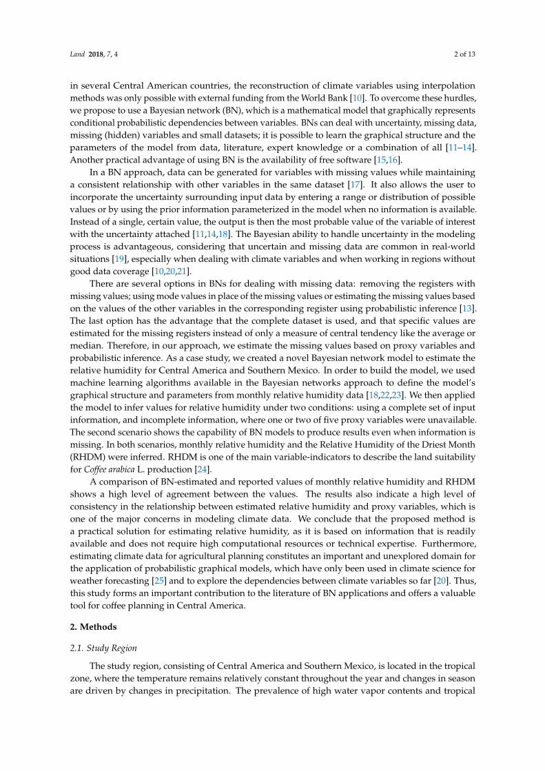
We downloaded a set of daily data of all variables, covering Central America and Southern Mexico(a total of 855 pixels) for the years 1979 to 2000. From this dataset, a monthly subset MRH was createdby aggregating the daily to monthly data for each year and pixel (n = 225,720). Then, a second subsetRHDM was created by extracting the data (cases) of all the variables for the driest months of eachyear (n = 18,810). Summary statistics for the variables of both datasets were calculated (Table A1):The data distribution for humidity is different in both datasets, with µ = 77.79 and 69.13, and σ = 9.66and 9.08 for the MRH and RDHM datasets, respectively, and in the RDHM dataset, the shape of thehumidity distribution is more skewed to the left (Figure 1). The distribution of precipitation alsodiffers markedly between both datasets (µ = 8.13 and 1.05, and σ = 8.38 and 1.79 for MRH and RDHMdatasets, respectively), whereas only minor difference can be found for solar radiation, maximum andminimum temperature, and wind speed.

1 https://globalweather.tamu.edu/

Land 2018, 7, 4 4 of 13Land 2018, 7, 4 4 of 13

Figure 1. Empirical distributions of monthly relative humidity, precipitation, maximum and minimum temperature, solar radiation and wind speed from the datasets MRH and RHDM (n = 225,270 and 18,810, respectively). MRH: Monthly Relative Humidity; RHDM: Relative Humidity of the Driest Month.

2.4. Variable Selection

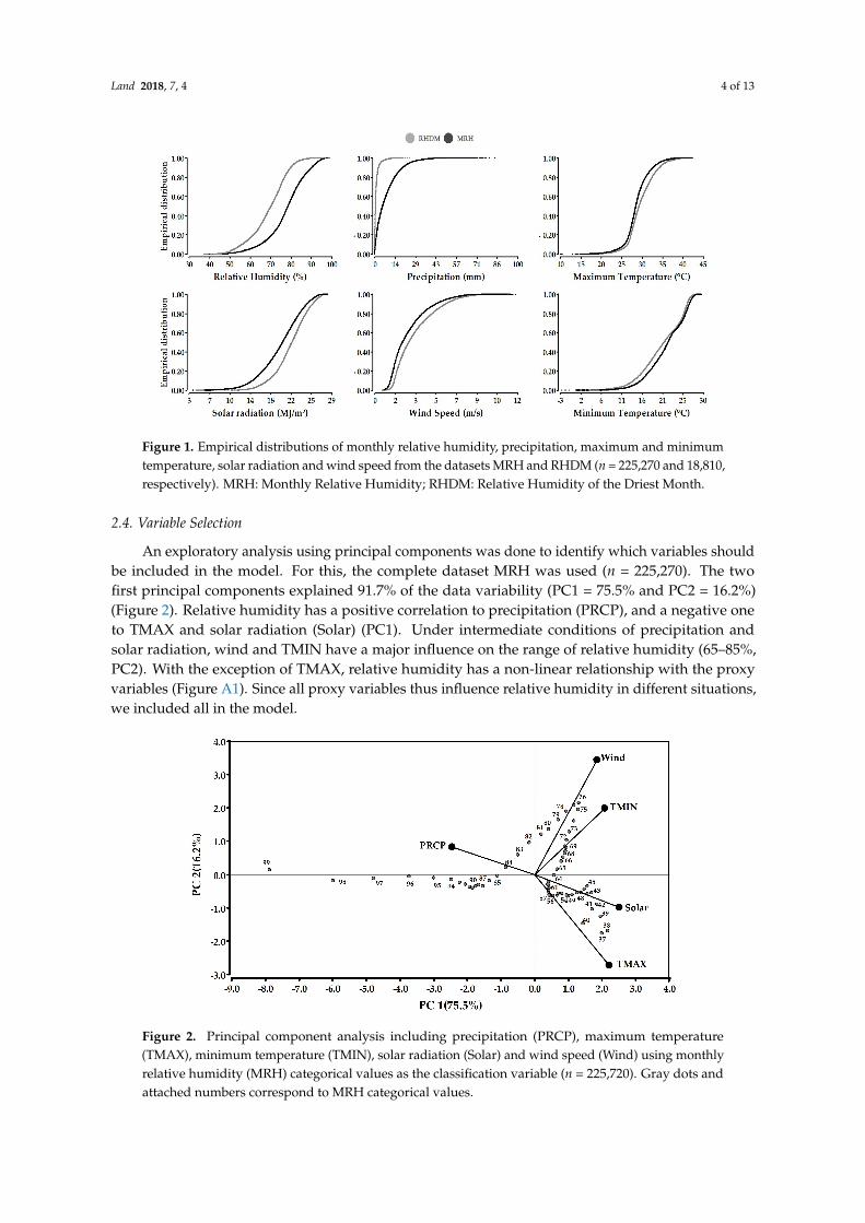
An exploratory analysis using principal components was done to identify which variables should be included in the model. For this, the complete dataset MRH was used (n = 225,270). The two first principal components explained 91.7% of the data variability (PC1 = 75.5% and PC2 =16.2%) (Figure 2). Relative humidity has a positive correlation to precipitation (PRCP), and a negative one to TMAX and solar radiation (Solar) (PC1). Under intermediate conditions of precipitation and solar radiation, wind and TMIN have a major influence on the range of relative humidity (65–85%, PC2). With the exception of TMAX, relative humidity has a non-linear relationship with the proxy variables (Figure A1). Since all proxy variables thus influence relative humidity in different situations, we included all in the model.

Figure 2. Principal component analysis including precipitation (PRCP), maximum temperature (TMAX), minimum temperature (TMIN), solar radiation (Solar) and wind speed (Wind) using monthly relative humidity (MRH) categorical values as the classification variable (n = 225,720). Gray dots and attached numbers correspond to MRH categorical values.

Figure 1. Empirical distributions of monthly relative humidity, precipitation, maximum and minimumtemperature, solar radiation and wind speed from the datasets MRH and RHDM (n = 225,270 and 18,810,respectively). MRH: Monthly Relative Humidity; RHDM: Relative Humidity of the Driest Month.

2.4. Variable Selection

An exploratory analysis using principal components was done to identify which variables shouldbe included in the model. For this, the complete dataset MRH was used (n = 225,270). The twofirst principal components explained 91.7% of the data variability (PC1 = 75.5% and PC2 = 16.2%)(Figure 2). Relative humidity has a positive correlation to precipitation (PRCP), and a negative oneto TMAX and solar radiation (Solar) (PC1). Under intermediate conditions of precipitation andsolar radiation, wind and TMIN have a major influence on the range of relative humidity (65–85%,PC2). With the exception of TMAX, relative humidity has a non-linear relationship with the proxyvariables (Figure A1). Since all proxy variables thus influence relative humidity in different situations,we included all in the model.

Land 2018, 7, 4 4 of 13

Figure 1. Empirical distributions of monthly relative humidity, precipitation, maximum and minimum temperature, solar radiation and wind speed from the datasets MRH and RHDM (n = 225,270 and 18,810, respectively). MRH: Monthly Relative Humidity; RHDM: Relative Humidity of the Driest Month.

2.4. Variable Selection

An exploratory analysis using principal components was done to identify which variables should be included in the model. For this, the complete dataset MRH was used (n = 225,270). The two first principal components explained 91.7% of the data variability (PC1 = 75.5% and PC2 =16.2%) (Figure 2). Relative humidity has a positive correlation to precipitation (PRCP), and a negative one to TMAX and solar radiation (Solar) (PC1). Under intermediate conditions of precipitation and solar radiation, wind and TMIN have a major influence on the range of relative humidity (65–85%, PC2). With the exception of TMAX, relative humidity has a non-linear relationship with the proxy variables (Figure A1). Since all proxy variables thus influence relative humidity in different situations, we included all in the model.

Figure 2. Principal component analysis including precipitation (PRCP), maximum temperature (TMAX), minimum temperature (TMIN), solar radiation (Solar) and wind speed (Wind) using monthly relative humidity (MRH) categorical values as the classification variable (n = 225,720). Gray dots and attached numbers correspond to MRH categorical values.

Figure 2. Principal component analysis including precipitation (PRCP), maximum temperature(TMAX), minimum temperature (TMIN), solar radiation (Solar) and wind speed (Wind) using monthlyrelative humidity (MRH) categorical values as the classification variable (n = 225,720). Gray dots andattached numbers correspond to MRH categorical values.

Land 2018, 7, 4 5 of 13

2.5. Discretization

The model was built using the software package Netica (Version 6.04, Norsys Software Corp.,Vancouver, BC, Canada), which is free for small models with less than 15 variables. For each selectedvariable, nodes were created and discretized. The discretization of continuous variables in BN leads tothe loss of information [11]. An accepted strategy to deal with this is to mimic the data distribution ofthe variables in the discretization [47,48]; however, the definition of the breakpoints for each state is amajor challenge [47,49,50]. There are automatic methods to discretize continuous variables, but theselection of one method over another based on their performance is not clear, and using automaticmethods may result in a discretization inappropriate for the purpose of the model and the users.For this reason, expert knowledge remains the best option for discretization [14,47,50].

Here, we seek to estimate monthly relative humidity and the relative humidity of the driest monthusing a single model. The data distribution for precipitation is narrower for RHDM than for MRH(Figure 1 & Table A1) and thus requires shorter breakpoints to gain enough precision to infer therelative humidity under dry conditions. We, therefore, split the states into two: for the lower valuesthat correspond to the data distribution of the cases2 of RHDM the breakpoints are shorter, and for theremaining range, the breakpoints are further apart. For the other proxy variables, intervals of equallength were implemented focusing on reproducing the distribution of the data. States were merged ifthe resulting states had a frequency distribution close to zero. The number of states of each variablewas also based on the level of influence of this variable on relative humidity (see Section 3.1.); the lessinfluence, the less states were defined, thus contributing to reducing model complexity without loss ofperformance (Figure 3).

We used the metric Spherical Payoff3 to evaluate the contribution of a change in range or thenumber of states on model performance. If a change in the state’s range or number of states performedbetter, the change remained.

2.6. Model Structure and Parameters

Once the node variables were discretized, the graphical model was learned from 80% of thecases of the dataset MRH (n = 180,530). The relative humidity node was set as the target variable,and the machine learning algorithm Tree Augmented Naive Bayes (TAN) was used to learn themodel structure (Figure 3). TAN is a Bayesian classifier that incorporates dependencies betweenattributes by building structures between them [22]. The TAN algorithm drew edges from relativehumidity to each proxy variable, and added extra edges between proxy variables. Using the same80% of the MRH dataset, the Bayesian Counting—Learning Algorithm [18] was used to learn theparameters –prior and conditional probabilities- of all variables in the model. The Counting—LearningAlgorithm allows the model to move from initial-ignorance mode to parameterized mode by calculatingthe conditional probabilities and experience (confidence of the conditional probabilities) of thecorresponding combination of variables’ states [18,23]. Once the parameter values are learned,the model can be compiled and is ready for use.

2 A case is the set of values of the proxy variables and relative humidity for a given month and pixel. For example, in theFigure 3B, the case entered in the net has values only for three variables.

3 The Spherical Payoff is a scoring metric used to test the performance of Bayesian network models. The score goes from 0 to1, where 1 indicates the best performance [51].

Land 2018, 7, 4 6 of 13Land 2018, 7, 4 6 of 13

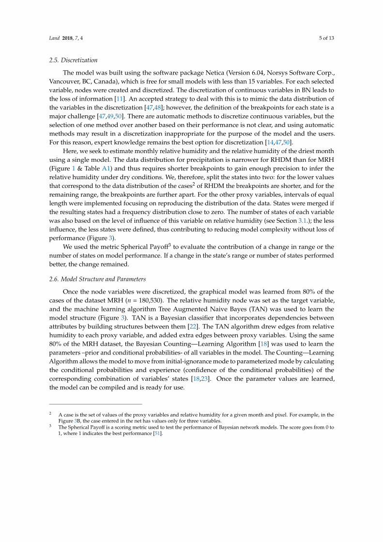
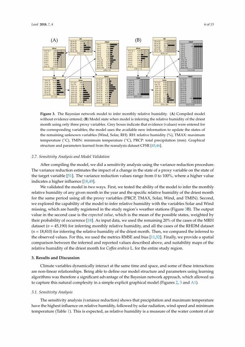
Figure 3. The Bayesian network model to infer monthly relative humidity. (A) Compiled model without evidence entered; (B) Model state when model is inferring the relative humidity of the driest month using only three proxy variables. Grey boxes indicate that evidence (values) were entered for the corresponding variables; the model uses the available new information to update the states of the remaining unknown variables (Wind, Solar, RH). RH: relative humidity (%), TMAX: maximum temperature (°C), TMIN: minimum temperature (°C), PRCP: total precipitation (mm). Graphical structure and parameters learned from the reanalysis dataset CFSR [45,46].

2.7. Sensitivity Analysis and Model Validation

After compiling the model, we did a sensitivity analysis using the variance reduction procedure. The variance reduction estimates the impact of a change in the state of a proxy variable on the state of the target variable [51]. The variance reduction values range from 0 to 100%, where a higher value indicates a higher influence [18,49].

We validated the model in two ways. First, we tested the ability of the model to infer the monthly relative humidity of any given month in the year and the specific relative humidity of the driest month for the same period using all the proxy variables (PRCP, TMAX, Solar, Wind, and TMIN). Second, we explored the capability of the model to infer relative humidity with the variables Solar and Wind missing, which are hardly registered in the study region’s weather stations (Figure 3B). The output value in the second case is the expected value, which is the mean of the possible states, weighted by their probability of occurrence [18]. As input data, we used the remaining 20% of the cases of the MRH dataset (n = 45,190) for inferring monthly relative humidity, and all the cases of the RHDM dataset (n = 18,810) for inferring the relative humidity of the driest month. Then, we compared the inferred to the observed values. For this, we used the metrics RMSE and bias [11,52]. Finally, we provide a spatial comparison between the inferred and reported values described above, and suitability maps of the relative humidity of the driest month for Coffea arabica L. for the entire study region.

3. Results and Discussion

Climate variables dynamically interact at the same time and space, and some of these interactions are non-linear relationships. Being able to define our model structure and parameters using learning algorithms was therefore a significant advantage of the Bayesian network approach, which allowed us to capture this natural complexity in a simple explicit graphical model (Figures 2, 3 and A1).

3.1. Sensitivity Analysis

The sensitivity analysis (variance reduction) shows that precipitation and maximum temperature have the highest influence on relative humidity, followed by solar radiation, wind speed

TMAX

0.1 to 2121 to 2525 to 2626 to 2727 to 2828 to 2929 to 3030 to 3131 to 3232 to 3333 to 3434 to 3535 to 43

0 0 0 0 0 0 0 0 0 0

100 0 0

33.5 ± 0.29

PRCP

0 to 11 to 22 to 33 to 44 to 55 to 66 to 88 to 1010 to 1515 to 2020 to 2525 to 3030 to 100

0 100

0 0 0 0 0 0 0 0 0 0 0

1.5 ± 0.29

RH

30 to 5050 to 6060 to 7070 to 8080 to 9090 to 100

2.344.2082.75.632.592.56

65.8 ± 8.1

Solar

0.1 to 55 to 1010 to 1212 to 1414 to 1616 to 1818 to 2020 to 2222 to 2424 to 2626 to 30

0.650.650.650.650.660.917.1011.722.244.210.7

23.4 ± 3.6

Wind

0.01 to 11 to 22 to 33 to 44 to 55 to 66 to 77 to 88 to 12

0.591.2115.643.825.27.893.341.840.54

3.92 ± 1.2

TMIN

-3 to 1515 to 1717 to 1919 to 2121 to 2323 to 2525 to 2727 to 30

0 0 0 0 0 0 0

10028.5 ± 0.87

(B)

TMAX

0.1 to 2121 to 2525 to 2626 to 2727 to 2828 to 2929 to 3030 to 3131 to 3232 to 3333 to 3434 to 3535 to 43

1.465.994.4810.517.819.213.08.266.014.563.332.163.24

28.7 ± 3.9

PRCP

0 to 11 to 22 to 33 to 44 to 55 to 66 to 88 to 1010 to 1515 to 2020 to 2525 to 3030 to 100

17.410.27.856.475.684.888.807.2213.88.314.602.392.46

8.92 ± 12

RH

30 to 5050 to 6060 to 7070 to 8080 to 9090 to 100

0.804.6113.338.332.910.0

77.8 ± 11

Solar

0.1 to 55 to 1010 to 1212 to 1414 to 1616 to 1818 to 2020 to 2222 to 2424 to 2626 to 30

.0391.191.944.869.5114.018.220.316.810.42.81

19.7 ± 4

Wind

0.01 to 11 to 22 to 33 to 44 to 55 to 66 to 77 to 88 to 12

1.8238.923.315.98.955.503.361.590.70

2.84 ± 1.7

TMIN

-3 to 1515 to 1717 to 1919 to 2121 to 2323 to 2525 to 2727 to 30

8.108.6511.613.817.411.421.17.87

21 ± 5.9

(A)

Figure 3. The Bayesian network model to infer monthly relative humidity. (A) Compiled modelwithout evidence entered; (B) Model state when model is inferring the relative humidity of the driestmonth using only three proxy variables. Grey boxes indicate that evidence (values) were entered forthe corresponding variables; the model uses the available new information to update the states ofthe remaining unknown variables (Wind, Solar, RH). RH: relative humidity (%), TMAX: maximumtemperature (◦C), TMIN: minimum temperature (◦C), PRCP: total precipitation (mm). Graphicalstructure and parameters learned from the reanalysis dataset CFSR [45,46].

2.7. Sensitivity Analysis and Model Validation

After compiling the model, we did a sensitivity analysis using the variance reduction procedure.The variance reduction estimates the impact of a change in the state of a proxy variable on the state ofthe target variable [51]. The variance reduction values range from 0 to 100%, where a higher valueindicates a higher influence [18,49].

We validated the model in two ways. First, we tested the ability of the model to infer the monthlyrelative humidity of any given month in the year and the specific relative humidity of the driest monthfor the same period using all the proxy variables (PRCP, TMAX, Solar, Wind, and TMIN). Second,we explored the capability of the model to infer relative humidity with the variables Solar and Windmissing, which are hardly registered in the study region’s weather stations (Figure 3B). The outputvalue in the second case is the expected value, which is the mean of the possible states, weighted bytheir probability of occurrence [18]. As input data, we used the remaining 20% of the cases of the MRHdataset (n = 45,190) for inferring monthly relative humidity, and all the cases of the RHDM dataset(n = 18,810) for inferring the relative humidity of the driest month. Then, we compared the inferred tothe observed values. For this, we used the metrics RMSE and bias [11,52]. Finally, we provide a spatialcomparison between the inferred and reported values described above, and suitability maps of therelative humidity of the driest month for Coffea arabica L. for the entire study region.

3. Results and Discussion

Climate variables dynamically interact at the same time and space, and some of these interactionsare non-linear relationships. Being able to define our model structure and parameters using learningalgorithms was therefore a significant advantage of the Bayesian network approach, which allowed usto capture this natural complexity in a simple explicit graphical model (Figures 2, 3 and A1).

3.1. Sensitivity Analysis

The sensitivity analysis (variance reduction) shows that precipitation and maximum temperaturehave the highest influence on relative humidity, followed by solar radiation, wind speed and minimumtemperature (Table 1). This is expected, as relative humidity is a measure of the water content of air

Land 2018, 7, 4 7 of 13

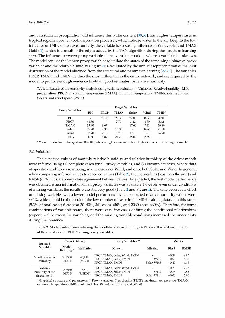
and variations in precipitation will influence this water content [39,53], and higher temperatures intropical regions boost evapotranspiration processes, which release water to the air. Despite the lowinfluence of TMIN on relative humidity, the variable has a strong influence on Wind, Solar and TMAX(Table 1), which is a result of the edges added by the TAN algorithm during the structure learningstep. The influence between proxy variables is relevant in situations where a variable is unknown.The model can use the known proxy variables to update the states of the remaining unknown proxyvariables and the relative humidity (Figure 3B), facilitated by the implicit representation of the jointdistribution of the model obtained from the structural and parameter learning [22,23]. The variablesPRCP, TMAX and TMIN are thus the most influential in the entire network, and are required by themodel to produce enough evidence to obtain good estimates for relative humidity.

Table 1. Results of the sensitivity analysis using variance reduction *. Variables: Relative humidity (RH),precipitation (PRCP), maximum temperature (TMAX), minimum temperature (TMIN), solar radiation(Solar), and wind speed (Wind).

Proxy VariablesTarget Variables

RH PRCP TMAX Solar Wind TMIN

RH - 25.20 29.30 22.80 18.50 4.68PRCP 41.80 - 7.70 3.22 0.89 5.42TMAX 33.90 6.67 - 17.60 7.41 29.60Solar 17.90 2.36 16.00 - 16.60 21.50Wind 13.70 2.18 1.73 19.10 - 24.90TMIN 1.94 3.09 24.20 28.60 45.90 -

* Variance reduction values go from 0 to 100, where a higher score indicates a higher influence on the target variable.

3.2. Validation

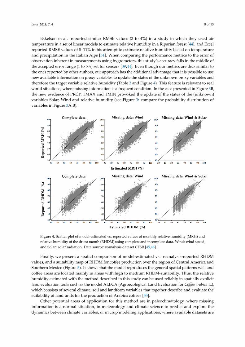
The expected values of monthly relative humidity and relative humidity of the driest monthwere inferred using (1) complete cases for all proxy variables, and (2) incomplete cases, where dataof specific variables were missing, in our case once Wind, and once both Solar and Wind. In general,when comparing inferred values to reported values (Table 2), the metrics bias (less than the unit) andRMSE (<5%) indicate a very close agreement between values. As expected, the best model performancewas obtained when information on all proxy variables was available; however, even under conditionsof missing variables, the results were still very good (Table 2 and Figure 4). The only observable effectof missing variables was a lower model performance when estimated relative humidity values were<60%, which could be the result of the low number of cases in the MRH training dataset in this range(5.3% of total cases; 6 cases at 30–40%, 361 cases <50%, and 2060 cases <60%). Therefore, for somecombinations of variable states, there were very few cases defining the conditional relationships(experience) between the variables, and the missing variable conditions increased the uncertaintyduring the inference.

Table 2. Model performance inferring the monthly relative humidity (MRH) and the relative humidityof the driest month (RHDM) using proxy variables.

InferredVariable

Cases (Dataset) Proxy Variables ** Metrics

ModelBuilding * Validation Known Missing BIAS RMSE

Monthly relativehumidity

180,530(MRH)

45,190(MRH)

PRCP, TMAX, Solar, Wind, TMIN - −0.99 4.03PRCP, TMAX, Solar, TMIN Wind −0.52 4.13PRCP, TMAX, TMIN Solar, Wind −0.40 4.13

Relativehumidity of the

driest month

180,530(MRH)

18,810(RHDM)

PRCP, TMAX, Solar, Wind, TMIN - −0.26 2.25PRCP, TMAX, Solar, TMIN Wind −0.76 4.93PRCP, TMAX, TMIN Solar, Wind −0.08 5.00

* Graphical structure and parameters. ** Proxy variables: Precipitation (PRCP), maximum temperature (TMAX),minimum temperature (TMIN), solar radiation (Solar), and wind speed (Wind).

Land 2018, 7, 4 8 of 13

Eskelson et al. reported similar RMSE values (3 to 4%) in a study in which they used airtemperature in a set of linear models to estimate relative humidity in a Riparian forest [44], and Eccelreported RMSE values of 8–11% in his attempt to estimate relative humidity based on temperatureand precipitation in the Italian Alps [54]. When comparing the performance metrics to the error ofobservation inherent in measurements using hygrometers, this study’s accuracy falls in the middle ofthe accepted error range (1 to 5%) set for sensors [39,44]. Even though our metrics are thus similar tothe ones reported by other authors, our approach has the additional advantage that it is possible to usenew available information on proxy variables to update the states of the unknown proxy variables andtherefore the target variable relative humidity (Table 2 and Figure 4). This feature is relevant to realworld situations, where missing information is a frequent condition. In the case presented in Figure 3B,the new evidence of PRCP, TMAX and TMIN provoked the update of the states of the (unknown)variables Solar, Wind and relative humidity (see Figure 3: compare the probability distribution ofvariables in Figure 3A,B).

Land 2018, 7, 4 8 of 13

the driest month

* Graphical structure and parameters. ** Proxy variables: Precipitation (PRCP), maximum temperature (TMAX), minimum temperature (TMIN), solar radiation (Solar), and wind speed (Wind).

Eskelson et al. reported similar RMSE values (3 to 4%) in a study in which they used air temperature in a set of linear models to estimate relative humidity in a Riparian forest [44], and Eccel reported RMSE values of 8–11% in his attempt to estimate relative humidity based on temperature and precipitation in the Italian Alps [54]. When comparing the performance metrics to the error of observation inherent in measurements using hygrometers, this study’s accuracy falls in the middle of the accepted error range (1 to 5%) set for sensors [39,44]. Even though our metrics are thus similar to the ones reported by other authors, our approach has the additional advantage that it is possible to use new available information on proxy variables to update the states of the unknown proxy variables and therefore the target variable relative humidity (Table 2 and Figure 4). This feature is relevant to real world situations, where missing information is a frequent condition. In the case presented in Figure 3B, the new evidence of PRCP, TMAX and TMIN provoked the update of the states of the (unknown) variables Solar, Wind and relative humidity (see Figure 3: compare the probability distribution of variables in Figure 3A,B).

Figure 4. Scatter plot of model-estimated vs. reported values of monthly relative humidity (MRH) and relative humidity of the driest month (RHDM) using complete and incomplete data. Wind: wind speed, and Solar: solar radiation. Data source: reanalysis dataset CFSR [45,46].

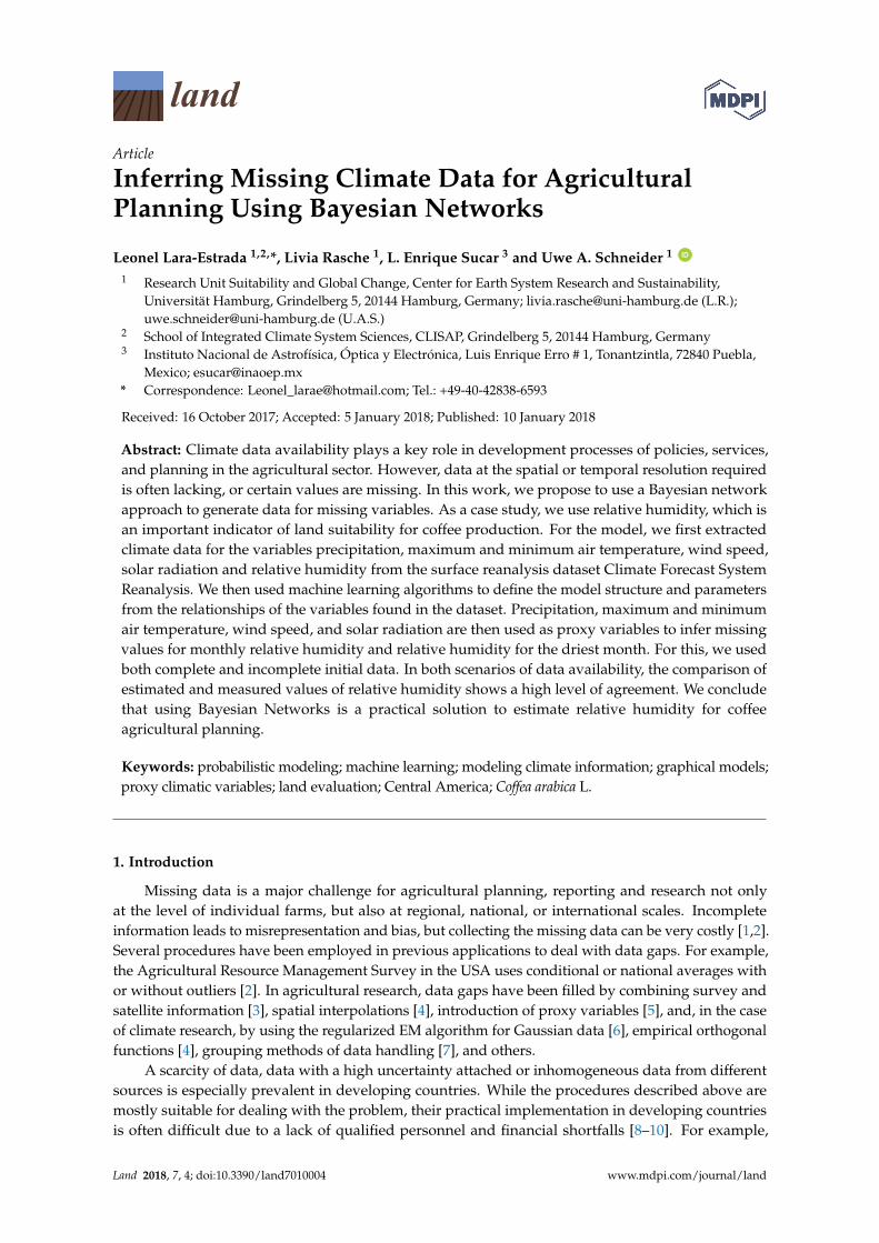
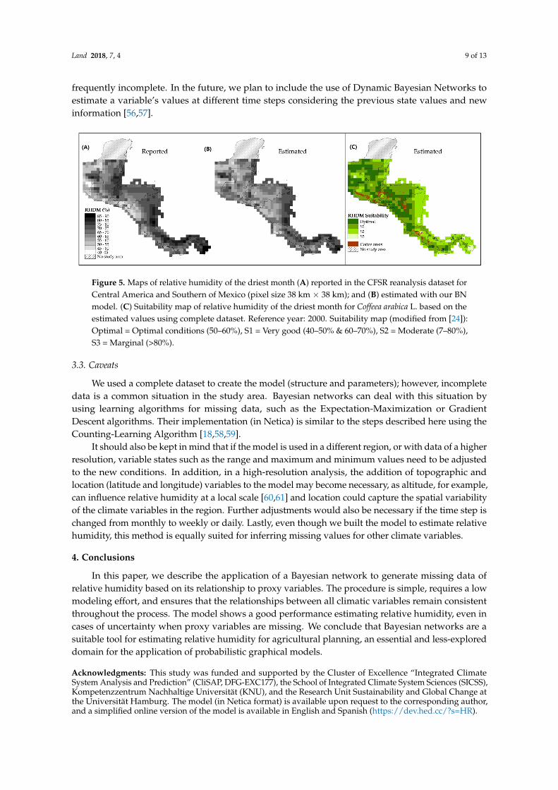
Finally, we present a spatial comparison of model-estimated vs. reanalysis-reported RHDM values, and a suitability map of RHDM for coffee production over the region of Central America and Southern Mexico (Figure 5). It shows that the model reproduces the general spatial patterns well and coffee areas are located mainly in areas with high to medium RHDM-suitability. Thus, the relative humidity estimated with the method described in this study can be used reliably in spatially explicit land evaluation tools such as the model ALECA (Agroecological Land Evaluation for Coffea arabica L.), which consists of several climate, soil and landform variables that together describe and evaluate the suitability of land units for the production of Arabica coffees [55].

Figure 4. Scatter plot of model-estimated vs. reported values of monthly relative humidity (MRH) andrelative humidity of the driest month (RHDM) using complete and incomplete data. Wind: wind speed,and Solar: solar radiation. Data source: reanalysis dataset CFSR [45,46].

Finally, we present a spatial comparison of model-estimated vs. reanalysis-reported RHDMvalues, and a suitability map of RHDM for coffee production over the region of Central America andSouthern Mexico (Figure 5). It shows that the model reproduces the general spatial patterns well andcoffee areas are located mainly in areas with high to medium RHDM-suitability. Thus, the relativehumidity estimated with the method described in this study can be used reliably in spatially explicitland evaluation tools such as the model ALECA (Agroecological Land Evaluation for Coffea arabica L.),which consists of several climate, soil and landform variables that together describe and evaluate thesuitability of land units for the production of Arabica coffees [55].

Other potential areas of application for this method are in paleoclimatology, where missinginformation is a normal situation, in meteorology and climate science to predict and explore thedynamics between climate variables, or in crop modeling applications, where available datasets are

Land 2018, 7, 4 9 of 13

frequently incomplete. In the future, we plan to include the use of Dynamic Bayesian Networks toestimate a variable’s values at different time steps considering the previous state values and newinformation [56,57].

Land 2018, 7, 4 9 of 13

Other potential areas of application for this method are in paleoclimatology, where missing information is a normal situation, in meteorology and climate science to predict and explore the dynamics between climate variables, or in crop modeling applications, where available datasets are frequently incomplete. In the future, we plan to include the use of Dynamic Bayesian Networks to estimate a variable’s values at different time steps considering the previous state values and new information [56,57].

Figure 5. Maps of relative humidity of the driest month (A) reported in the CFSR reanalysis dataset for Central America and Southern of Mexico (pixel size 38 km × 38 km); and (B) estimated with our BN model. (C) Suitability map of relative humidity of the driest month for Coffeea arabica L. based on the estimated values using complete dataset. Reference year: 2000. Suitability map (modified from [24]): Optimal = Optimal conditions (50–60%), S1 = Very good (40–50% & 60–70%), S2 = Moderate (7–80%), S3 = Marginal (>80%).

3.3. Caveats

We used a complete dataset to create the model (structure and parameters); however, incomplete data is a common situation in the study area. Bayesian networks can deal with this situation by using learning algorithms for missing data, such as the Expectation-Maximization or Gradient Descent algorithms. Their implementation (in Netica) is similar to the steps described here using the Counting-Learning Algorithm [18,58,59].

It should also be kept in mind that if the model is used in a different region, or with data of a higher resolution, variable states such as the range and maximum and minimum values need to be adjusted to the new conditions. In addition, in a high-resolution analysis, the addition of topographic and location (latitude and longitude) variables to the model may become necessary, as altitude, for example, can influence relative humidity at a local scale [60,61] and location could capture the spatial variability of the climate variables in the region. Further adjustments would also be necessary if the time step is changed from monthly to weekly or daily. Lastly, even though we built the model to estimate relative humidity, this method is equally suited for inferring missing values for other climate variables.

4. Conclusions

In this paper, we describe the application of a Bayesian network to generate missing data of relative humidity based on its relationship to proxy variables. The procedure is simple, requires a low modeling effort, and ensures that the relationships between all climatic variables remain consistent throughout the process. The model shows a good performance estimating relative humidity, even in cases of uncertainty when proxy variables are missing. We conclude that Bayesian networks are a suitable tool for estimating relative humidity for agricultural planning, an essential and less-explored domain for the application of probabilistic graphical models.

Figure 5. Maps of relative humidity of the driest month (A) reported in the CFSR reanalysis dataset forCentral America and Southern of Mexico (pixel size 38 km × 38 km); and (B) estimated with our BNmodel. (C) Suitability map of relative humidity of the driest month for Coffeea arabica L. based on theestimated values using complete dataset. Reference year: 2000. Suitability map (modified from [24]):Optimal = Optimal conditions (50–60%), S1 = Very good (40–50% & 60–70%), S2 = Moderate (7–80%),S3 = Marginal (>80%).

3.3. Caveats

We used a complete dataset to create the model (structure and parameters); however, incompletedata is a common situation in the study area. Bayesian networks can deal with this situation byusing learning algorithms for missing data, such as the Expectation-Maximization or GradientDescent algorithms. Their implementation (in Netica) is similar to the steps described here using theCounting-Learning Algorithm [18,58,59].

It should also be kept in mind that if the model is used in a different region, or with data of a higherresolution, variable states such as the range and maximum and minimum values need to be adjustedto the new conditions. In addition, in a high-resolution analysis, the addition of topographic andlocation (latitude and longitude) variables to the model may become necessary, as altitude, for example,can influence relative humidity at a local scale [60,61] and location could capture the spatial variabilityof the climate variables in the region. Further adjustments would also be necessary if the time step ischanged from monthly to weekly or daily. Lastly, even though we built the model to estimate relativehumidity, this method is equally suited for inferring missing values for other climate variables.

4. Conclusions

In this paper, we describe the application of a Bayesian network to generate missing data ofrelative humidity based on its relationship to proxy variables. The procedure is simple, requires a lowmodeling effort, and ensures that the relationships between all climatic variables remain consistentthroughout the process. The model shows a good performance estimating relative humidity, even incases of uncertainty when proxy variables are missing. We conclude that Bayesian networks are asuitable tool for estimating relative humidity for agricultural planning, an essential and less-exploreddomain for the application of probabilistic graphical models.

Acknowledgments: This study was funded and supported by the Cluster of Excellence “Integrated ClimateSystem Analysis and Prediction” (CliSAP, DFG-EXC177), the School of Integrated Climate System Sciences (SICSS),Kompetenzzentrum Nachhaltige Universität (KNU), and the Research Unit Sustainability and Global Change atthe Universität Hamburg. The model (in Netica format) is available upon request to the corresponding author,and a simplified online version of the model is available in English and Spanish (https://dev.hed.cc/?s=HR).

Land 2018, 7, 4 10 of 13

Author Contributions: Leonel Lara conceived, designed, developed, and performed the modeling and wrote thepaper. Livia Rasche, Uwe Schneider, and L. Enrique Sucar supported the modeling performance analysis and thewriting processes. Livia Rasche edited the paper. Uwe Schneider contributed with materials and analysis tools.

Conflicts of Interest: The authors declare no conflict of interest.

Appendix A

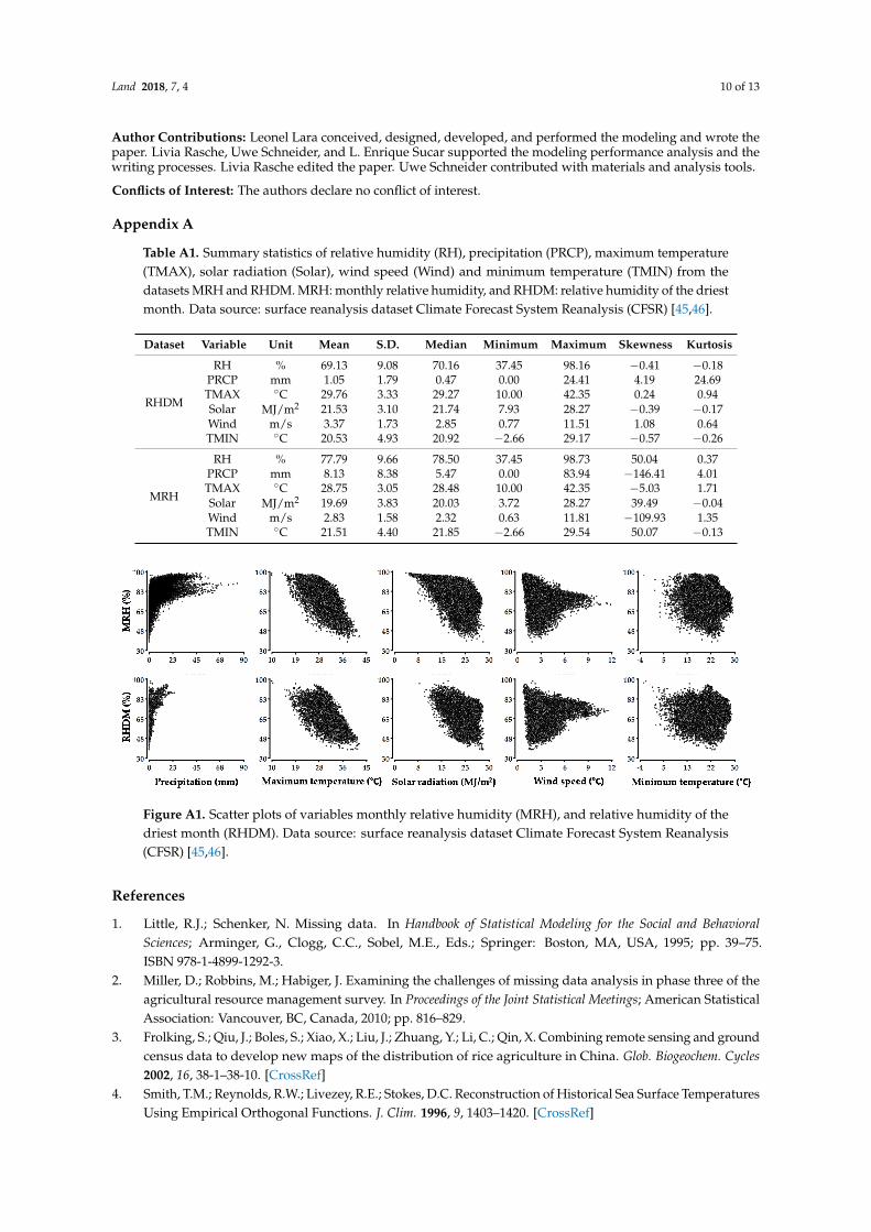
Table A1. Summary statistics of relative humidity (RH), precipitation (PRCP), maximum temperature(TMAX), solar radiation (Solar), wind speed (Wind) and minimum temperature (TMIN) from thedatasets MRH and RHDM. MRH: monthly relative humidity, and RHDM: relative humidity of the driestmonth. Data source: surface reanalysis dataset Climate Forecast System Reanalysis (CFSR) [45,46].

Dataset Variable Unit Mean S.D. Median Minimum Maximum Skewness Kurtosis

RHDM

RH % 69.13 9.08 70.16 37.45 98.16 −0.41 −0.18PRCP mm 1.05 1.79 0.47 0.00 24.41 4.19 24.69TMAX ◦C 29.76 3.33 29.27 10.00 42.35 0.24 0.94Solar MJ/m2 21.53 3.10 21.74 7.93 28.27 −0.39 −0.17Wind m/s 3.37 1.73 2.85 0.77 11.51 1.08 0.64TMIN ◦C 20.53 4.93 20.92 −2.66 29.17 −0.57 −0.26

MRH

RH % 77.79 9.66 78.50 37.45 98.73 50.04 0.37PRCP mm 8.13 8.38 5.47 0.00 83.94 −146.41 4.01TMAX ◦C 28.75 3.05 28.48 10.00 42.35 −5.03 1.71Solar MJ/m2 19.69 3.83 20.03 3.72 28.27 39.49 −0.04Wind m/s 2.83 1.58 2.32 0.63 11.81 −109.93 1.35TMIN ◦C 21.51 4.40 21.85 −2.66 29.54 50.07 −0.13

Land 2018, 7, 4 10 of 13

Acknowledgments: This study was funded and supported by the Cluster of Excellence “Integrated Climate System Analysis and Prediction” (CliSAP, DFG-EXC177), the School of Integrated Climate System Sciences (SICSS), Kompetenzzentrum Nachhaltige Universität (KNU), and the Research Unit Sustainability and Global Change at the Universität Hamburg. The model (in Netica format) is available upon request to the corresponding author, and a simplified online version of the model is available in English and Spanish (https://dev.hed.cc/?s=HR).

Author Contributions: Leonel Lara conceived, designed, developed, and performed the modeling and wrote the paper. Livia Rasche, Uwe Schneider, and L. Enrique Sucar supported the modeling performance analysis and the writing processes. Livia Rasche edited the paper. Uwe Schneider contributed with materials and analysis tools.

Conflicts of Interest: The authors declare no conflict of interest.

Appendix A

Table A1. Summary statistics of relative humidity (RH), precipitation (PRCP), maximum temperature (TMAX), solar radiation (Solar), wind speed (Wind) and minimum temperature (TMIN) from the datasets MRH and RHDM. MRH: monthly relative humidity, and RHDM: relative humidity of the driest month. Data source: surface reanalysis dataset Climate Forecast System Reanalysis (CFSR) [45,46].

Dataset Variable Unit Mean S.D. Median Minimum Maximum Skewness Kurtosis

RHDM

RH % 69.13 9.08 70.16 37.45 98.16 −0.41 −0.18 PRCP mm 1.05 1.79 0.47 0.00 24.41 4.19 24.69 TMAX °C 29.76 3.33 29.27 10.00 42.35 0.24 0.94 Solar MJ/m2 21.53 3.10 21.74 7.93 28.27 −0.39 −0.17 Wind m/s 3.37 1.73 2.85 0.77 11.51 1.08 0.64 TMIN °C 20.53 4.93 20.92 −2.66 29.17 −0.57 −0.26

MRH

RH % 77.79 9.66 78.50 37.45 98.73 50.04 0.37 PRCP mm 8.13 8.38 5.47 0.00 83.94 −146.41 4.01 TMAX °C 28.75 3.05 28.48 10.00 42.35 −5.03 1.71 Solar MJ/m2 19.69 3.83 20.03 3.72 28.27 39.49 −0.04 Wind m/s 2.83 1.58 2.32 0.63 11.81 −109.93 1.35 TMIN °C 21.51 4.40 21.85 −2.66 29.54 50.07 −0.13

Figure A1. Scatter plots of variables monthly relative humidity (MRH), and relative humidity of the driest month (RHDM). Data source: surface reanalysis dataset Climate Forecast System Reanalysis (CFSR) [45,46].

References

1. Little, R.J.; Schenker, N. Missing data. In Handbook of Statistical Modeling for the Social and Behavioral Sciences; Arminger, G., Clogg, C.C., Sobel, M.E., Eds.; Springer: Boston, MA, USA, 1995; pp. 39–75, ISBN 978-1-4899-1292-3.

Figure A1. Scatter plots of variables monthly relative humidity (MRH), and relative humidity of thedriest month (RHDM). Data source: surface reanalysis dataset Climate Forecast System Reanalysis(CFSR) [45,46].

References

1. Little, R.J.; Schenker, N. Missing data. In Handbook of Statistical Modeling for the Social and BehavioralSciences; Arminger, G., Clogg, C.C., Sobel, M.E., Eds.; Springer: Boston, MA, USA, 1995; pp. 39–75.ISBN 978-1-4899-1292-3.

2. Miller, D.; Robbins, M.; Habiger, J. Examining the challenges of missing data analysis in phase three of theagricultural resource management survey. In Proceedings of the Joint Statistical Meetings; American StatisticalAssociation: Vancouver, BC, Canada, 2010; pp. 816–829.

3. Frolking, S.; Qiu, J.; Boles, S.; Xiao, X.; Liu, J.; Zhuang, Y.; Li, C.; Qin, X. Combining remote sensing and groundcensus data to develop new maps of the distribution of rice agriculture in China. Glob. Biogeochem. Cycles2002, 16, 38-1–38-10. [CrossRef]

4. Smith, T.M.; Reynolds, R.W.; Livezey, R.E.; Stokes, D.C. Reconstruction of Historical Sea Surface TemperaturesUsing Empirical Orthogonal Functions. J. Clim. 1996, 9, 1403–1420. [CrossRef]

Land 2018, 7, 4 11 of 13

5. Liu, D.L.; Scott, B.J. Estimation of solar radiation in Australia from rainfall and temperature observations.Agric. For. Meteorol. 2001, 106, 41–59. [CrossRef]

6. Schneider, T. Analysis of incomplete climate data: Estimation of mean values and covariance matrices andimputation of missing values. J. Clim. 2001, 14, 853–871. [CrossRef]

7. Acock, M.C.; Pachepsky, Y.A. Estimating missing weather data for agricultural simulations using groupmethod of data handling. J. Appl. Meteorol. 2000, 39, 1176–1184. [CrossRef]

8. Harris, E. Building scientific capacity in developing countries. EMBO Rep. 2004, 5, 7–11. [CrossRef] [PubMed]9. Wagner, C.S.; Brahmakulam, I.; Jackson, B.; Wong, A.; Yoda, T. Science and Technology Collaboration: Building

Capability in Developing Countries; RAND: Pittsburgh, PA, USA, 2001; p. 102.10. World Bank. Weather Data Grids for Agriculture Risk Management: The Case of Honduras and Guatemala;

The World Bank: Washington, DC, USA, 2013; pp. 1–44.11. Aguilera, P.A.; Fernández, A.; Fernández, R.; Rumí, R.; Salmerón, A. Bayesian networks in environmental

modelling. Environ. Model. Softw. 2011, 26, 1376–1388. [CrossRef]12. Barton, D.N.; Kuikka, S.; Varis, O.; Uusitalo, L.; Henriksen, H.J.; Borsuk, M.; de la Hera, A.; Farmani, R.;

Johnson, S.; Linnell, J.D. Bayesian networks in environmental and resource management. Integr. Environ.Assess. Manag. 2012, 8, 418–429. [CrossRef] [PubMed]

13. Sucar, L.E. Probabilistic Graphical Models: Principles and Applications; Advances in Computer Vision and PatternRecognition; Springer: London, UK; Heidelberg, Germany; New York, NY, USA; Dordrecht, The Netherlands,2015; ISBN 978-1-4471-6699-3.

14. Uusitalo, L. Advantages and challenges of Bayesian networks in environmental modelling. Ecol. Model. 2007,203, 312–318. [CrossRef]

15. Kevin Murphy Software Packages for Graphical Models. Available online: http://www.cs.ubc.ca/~murphyk/Software/bnsoft.html (accessed on 26 July 2017).

16. Mahjoub, M.A.; Kalti, K. Software Comparison Dealing with Bayesian Networks. In Advances in NeuralNetworks—ISNN 2011; Liu, D., Zhang, H., Polycarpou, M., Alippi, C., He, H., Eds.; Lecture Notes in ComputerScience; Springer: Berlin/Heidelberg, Germany, 2011; pp. 168–177, ISBN 978-3-642-21110-2.

17. Cano, R.; Sordo, C.; Gutiérrez, J.M. Applications of Bayesian networks in meteorology. In Advances inBayesian Networks; Springer: Berlin, Germany, 2004; pp. 309–328, ISBN 978-3-540-39879-0.

18. Norsys Netica Help. Available online: http://www.norsys.com/WebHelp/NETICA.htm (accessed on15 September 2015).

19. Andradóttir, S.; Bier, V.M. Applying Bayesian ideas in simulation. Simul. Pract. Theory 2000, 8, 253–280.[CrossRef]

20. De la Torre-Gea, G.; Soto-Zarazúa, G.M.; Guevara-González, R.; Rico-García, E. Bayesian networks fordefining relationships among climate factors. Int. J. Phys. Sci. 2011, 6, 4412–4418. [CrossRef]

21. Fang, L.; Qing-Cun, Z.; Chao-Fan, L. A Bayesian Scheme for Probabilistic Multi-Model Ensemble Predictionof Summer Rainfall over the Yangtze River Valley. Atmos. Ocean. Sci. Lett. 2009, 2, 314–319. [CrossRef]

22. Friedman, N.; Geiger, D.; Goldszmidt, M. Bayesian Network Classifiers. Mach. Learn. 1997, 29, 131–163.[CrossRef]

23. Spiegelhalter, D.J.; Dawid, A.P.; Lauritzen, S.L.; Cowell, R.G. Bayesian Analysis in Expert Systems. Stat. Sci.1993, 8, 219–247. [CrossRef]

24. Descroix, F.; Snoeck, J. Enviromental Factors Suitable for Coffee Cultivation. In Coffee: Growing, Processing,Sustainable Production: A Guidebook for Growers, Processors, Traders, and Researchers; Wintgens, J.N., Ed.;Wiley-VCH Verlag GmbH: Weinheim, Germany, 2004; pp. 164–177, ISBN 978-3-527-61962-7.

25. Cofiño, A.; Cano, R.; Sordo, C.; Gutierrez, J. Bayesian Networks for Probabilistic Weather Prediction.In Proceedings of the 15th European Conference on Artificial Intelligence (ECAI 2002); IOS Press: Lyon, France,2002; pp. 675–700.

26. Peixoto, J.; Oort, A.H. The Climatology of Relative Humidity in the Atmosphere. J. Clim. 1996, 9, 3443–3463.[CrossRef]

27. Taylor, M.A.; Alfaro, E.J. Central America and the Caribbean, Climate of. In Encyclopedia of World Climatology;Oliver, J., Ed.; Encyclopedia of Earth Sciences Series; Springer: Dordrecht, The Netherlands, 2005; pp. 183–189.ISBN 978-1-4020-3266-0.

Land 2018, 7, 4 12 of 13

28. Avelino, J.; Perriot, J.J.; Guyot, B.; Decazy, F.; Cilas, C. Identifying terroir coffees in Honduras. In Recherche etCaféiculture = Research and Coffee Growing; CIRADP-CP-CAFE, Ed.; Plantations, Recherche, Développement;CIRAD-CP: Montpellier, France, 2002; pp. 6–16.

29. Avelino, J.; Barboza, B.; Araya, J.C.; Fonseca, C.; Davrieux, F.; Guyot, B.; Cilas, C. Effects of slope exposure,altitude and yield on coffee quality in two altitude terroirs of Costa Rica, Orosi and Santa María de Dota.J. Sci. Food Agric. 2005, 85, 1869–1876. [CrossRef]

30. Bertrand, B.; Vaast, P.; Alpizar, E.; Etienne, H.; Davrieux, F.; Charmetant, P. Comparison of bean biochemicalcomposition and beverage quality of Arabica hybrids involving Sudanese-Ethiopian origins with traditionalvarieties at various elevations in Central America. Tree Physiol. 2006, 26, 1239–1248. [CrossRef] [PubMed]

31. Vaast, P.; Cilas, C.; Perriot, J.J.; Davrieux, J.J.; Guyot, B.; Bolaños, M. Mapping of coffee quality in Nicaraguaaccording to regions, ecological conditions and farm management. In Proceedings of the 20th InternationalConference on Coffee Science; ASIC: Bangalore, India, 2004; pp. 842–850.

32. Somarriba, E.; Harvey, C.A.; Samper, M.; Anthony, F.; González, J.; Staver, C.; Rice, R.A. BiodiversityConservation in Neotropical Coffee (Coffea arabica L.) Plantations. In Agroforestry and Biodiversity Conservationin Tropical Landscapes; Schroth, G., da Fonseca, G., Harvey, C., Gascon, C., Vasconcelos, H., Izac, A., Eds.;Island Press: Washington, DC, USA, 2004; pp. 198–226, ISBN 978-1-59726-744-1.

33. Bertrand, B.; Rapidel, B. (Eds.) Desafíos de la Caficultura en Centroamérica; IICA, PROMECAFE: San José, CR,USA, 1999; ISBN 978-92-9039-391-7.

34. ICO Historical Data on the Global Coffee Trade. Available online: http://www.ico.org/new_historical.asp?section=Statistics (accessed on 11 September 2015).

35. Gay, C.; Estrada, F.; Conde, C.; Eakin, H.; Villers, L. Potential Impacts of Climate Change on Agriculture:A Case of Study of Coffee Production in Veracruz, Mexico. Clim. Chang. 2006, 79, 259–288. [CrossRef]

36. Haggar, J.; Schepp, K. Coffee and Climate Change: Impacts and Options for Adaption in Brazil, Guatemala, Tanzaniaand Vietnam; NRI Working Paper Series; NRI, University of Greenwich: London, UK, 2012; p. 51.

37. Läderach, P.; Lundy, M.; Jarvis, A.; Ramirez, J.; Portilla, E.P.; Schepp, K.; Eitzinger, A. Predicted Impact ofClimate Change on Coffee Supply Chains. In The Economic, Social and Political Elements of Climate Change;Leal Filho, W., Ed.; Climate Change Management; Springer: Berlin/Heidelberg, Germany, 2010; pp. 703–723.ISBN 978-3-642-14776-0.

38. Primault, B. Transfer of Quantities of Air Masses. In Agrometeorology; Springer: Berlin/Heidelberg, Germany,1979; pp. 46–61, ISBN 978-3-642-67290-3.

39. Harrison, R.G. Humidity. In Meteorological Measurements and Instrumentation; Advancing Weather andClimate Science Series; John Wiley & Sons, Ltd.: Chichester, UK, 2014; pp. 103–122, ISBN 978-1-118-74579-3.

40. Lawrence, M.G. The Relationship between Relative Humidity and the Dewpoint Temperature in Moist Air:A Simple Conversion and Applications. Bull. Am. Meteorol. Soc. 2005, 86, 225–233. [CrossRef]

41. Ribeiro, F.C.; Borém, F.M.; Giomo, G.S.; De Lima, R.R.; Malta, M.R.; Figueiredo, L.P. Storage of green coffeein hermetic packaging injected with CO2. J. Stored Prod. Res. 2011, 47, 341–348. [CrossRef]

42. Rojas, J. Green Coffee Storage. In Coffee: Growing, Processing, Sustainable Production: A Guidebook for Growers,Processors, Traders, and Researchers; Wintgens, J.N., Ed.; Wiley-VCH Verlag GmbH: Weinheim, Germany, 2004;pp. 733–750, ISBN 978-3-527-61962-7.

43. DaMatta, F.; Ronchi, C.; Maestri, M.; Barros, R.S. Ecophysiology of coffee growth and production. Braz. J.Plant Physiol. 2007, 19, 485–510. [CrossRef]

44. Eskelson, B.N.I.; Anderson, P.D.; Temesgen, H. Modeling Relative Humidity in Headwater Forests usingCorrelation with Air Temperature. Northwest Sci. 2013, 87, 40–58. [CrossRef]

45. Fuka, D.R.; Walter, M.T.; MacAlister, C.; Degaetano, A.T.; Steenhuis, T.S.; Easton, Z.M. Using the ClimateForecast System Reanalysis as weather input data for watershed models: Using cfsr as weather input datafor watershed models. Hydrol. Process. 2014, 28, 5613–5623. [CrossRef]

46. Saha, S.; Moorthi, S.; Pan, H.-L.; Wu, X.; Wang, J.; Nadiga, S.; Tripp, P.; Kistler, R.; Woollen, J.; Behringer, D.;et al. The NCEP Climate Forecast System Reanalysis. Bull. Am. Meteorol. Soc. 2010, 91, 1015–1057. [CrossRef]

47. Nojavan, A.F.; Qian, S.S.; Stow, C.A. Comparative analysis of discretization methods in Bayesian networks.Environ. Model. Softw. 2017, 87, 64–71. [CrossRef]

48. Allan, J.D.; Yuan, L.L.; Black, P.; Stockton, T.; Davies, P.E.; Magierowski, R.H.; Read, S.M. Investigatingthe relationships between environmental stressors and stream condition using Bayesian belief networks.Freshw. Biol. 2012, 57, 58–73. [CrossRef]

Land 2018, 7, 4 13 of 13

49. Marcot, B.G.; Steventon, J.D.; Sutherland, G.D.; McCann, R.K. Guidelines for developing and updatingBayesian belief networks applied to ecological modeling and conservation. Can. J. For. Res. 2006, 36,3063–3074. [CrossRef]

50. McCann, R.K.; Marcot, B.G.; Ellis, R. Bayesian belief networks: Applications in ecology and natural resourcemanagement. Can. J. For. Res. 2006, 36, 3053–3062. [CrossRef]

51. Marcot, B.G. Metrics for evaluating performance and uncertainty of Bayesian network models. Ecol. Model.2012, 230, 50–62. [CrossRef]

52. Badescu, V. Use of Willmott’s index of agreement to the validation of meteorological models. Meteorol. Mag.1993, 122, 282–286.

53. Magaña, V.; Amador, J.A.; Medina, S. The midsummer drought over Mexico and Central America. J. Clim.1999, 12, 1577–1588. [CrossRef]

54. Eccel, E. Estimating air humidity from temperature and precipitation measures for modelling applications.Meteorol. Appl. 2012, 19, 118–128. [CrossRef]

55. Lara-Estrada, L.; Rasche, L.; Schneider, U.A. Modeling land suitability for Coffea arabica L. in Central America.Environ. Model. Softw. 2017, 95, 196–209. [CrossRef]

56. Ghahramani, Z. Learning dynamic Bayesian networks. In Adaptive Processing of Sequences and Data Structures;Giles, C.L., Gori, M., Eds.; Lecture Notes in Computer Science; Springer: Berlin, Germany, 1998; pp. 168–197,ISBN 978-3-540-69752-7.

57. Ibargüengoytia, P.H.; Garcıa, U.A.; Herrera-Vega, J.; Hernández-Leal, P.; Morales, E.F.; Sucar, L.E.;Orihuela-Espina, F.; Erro, L.E. On the Estimation of Missing Data in Incomplete Databases: AutoregressiveBayesian Networks. In Proceeding of the Eighth International Conference on Systems (ICONS 2013); Ege, R.,Koszalka, L., Eds.; IARA: Seville, Spain, 2013; pp. 111–116.

58. Sucar, L.E. Bayesian Networks: Learning. In Probabilistic Graphical Models; Springer: London, UK, 2015;pp. 137–159, ISBN 978-1-4471-6698-6.

59. Korb, K.B.; Nicholson, A. Bayesian Artificial Intelligence, 2nd ed.; Chapman & Hall/CRC Computer Scienceand Data Analysis Series; CRC Press: Boca Raton, FL, USA, 2011; ISBN 978-1-4398-1591-5.

60. Fries, A.; Rollenbeck, R.; Nauß, T.; Peters, T.; Bendix, J. Near surface air humidity in a megadiverse Andeanmountain ecosystem of southern Ecuador and its regionalization. Agric. For. Meteorol. 2012, 152, 17–30.[CrossRef]

61. Romps, D.M. An Analytical Model for Tropical Relative Humidity. J. Clim. 2014, 27, 7432–7449. [CrossRef]

© 2018 by the authors. Licensee MDPI, Basel, Switzerland. This article is an open accessarticle distributed under the terms and conditions of the Creative Commons Attribution(CC BY) license (http://creativecommons.org/licenses/by/4.0/).