Embed Size (px)
Citation preview
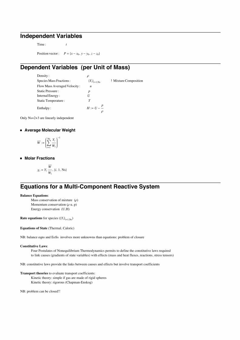
Independent VariablesTime : t
Position vector : P = 8x - x0, y- y0, z- z0<
Dependent Variables (per Unit of Mass)Density : r
Species Mass Fractions : 8Yi<i=1,Ns ! Mixture CompositionFlow Mass Averaged Velocity : uStatic Pressure : pInternal Energy : UStatic Temperature : T
Enthalpy : H := U -p
r
Only Ns+2+3 are linearly independent
ü Average Molecular Weight
W := ‚i=1
Ns YiWi
-1
ü Molar Fractions
ci = Yi W
Wi, 8i, 1, Ns<
Equations for a Multi-Component Reactive SystemBalance Equations:
Mass conservation of mixture (r)Momentum conservation (r u, p)Energy conservation (U,H)
Rate equations for species (8Yi<i=1,Ns)
Equations of State (Thermal, Caloric)
NB: balance eqns and EoSs involves more unknowns than equations: problem of closure
Constitutive Laws:Four Postulates of Nonequilibrium Thermodynamics permits to define the constitutive laws requiredto link causes (gradients of state variables) with effects (mass and heat fluxes, reactions, stress tensors)
NB: constitutive laws provide the links between causes and effects but involve transport coefficients
Transport theories to evaluate transport coefficients:Kinetic theory: simple if gas are made of rigid spheresKinetic theory: rigorous (Chapman-Enskog)
NB: problem can be closed!!

Velocity and Fluxes in Multi-Component Mixtures
ü Velocities
Absolute velocity of species : u j
Average Velocities
Average Velocity per Units of Mass : u =I⁄j=1Ns r j u jM
rwith r = ‚
j=1
Ns
r j
Average Velocity per Units of Mole : u* =I⁄j=1Ns c j u jMc
with c = ‚j=1
Ns
c j
Diffusion VelocitiesRelative Velocity per Units of Mass : V j = u j - uRelative Velocity per Units of Mole : V j
* = u j - u*
ü Fluxes
Absolute Mass Flux of species : m° j = r j u jAbsolute Molar Flux of species : n° j = c j u j
Relative Mass Flux of species : J j = r j Iu j - uM = r j V j with ‚j=1
Ns
J j = 0
Relative Molar Flux of species : J j* = c j Iu j - u*M = c j V j* with ‚
j=1
Ns
J j* = 0
Balance Equations
ü Eulerian Formulation (balance equation for a control volume fixed in space)
ü Integral Form
∂t‡V
Ñ
j „V = -‡V
Ñ
“ .@fD „V +‡V
Ñ
wj „V = -‡S=∂V
Ñ
f . n „S +‡V
Ñ
wj „V j œ R; f œ RN
∂t‡V
Ñ
f „V = -‡V
Ñ
“ .@TD „V +‡V
Ñ
w f „V = -‡S=∂V
Ñ
T . n „S +‡V
Ñ
w f „V f œ RN; T œ RNxN
ü Differential Form
∂tHjL = -“.@fD + wj j œ R; f œ RN
∂tH fL = -“.@TD + wf f œ RN; T œ RNxN
2 SummaryMCEqns.nb

ü Conservation Laws
Species Mass Evolution : j = r j = rY j ï ∂t IrY jM = -“ .AN jE + w j
Momentum conservation : f = r u u œ R3 ï ∂t H r uL = -“ .@QD +‚j=1
Ns
r j g j
Energy conservation : j = r U +1
2 u. u ï ∂t r U +
1
2 u. u = -“ .@ED +‚
j=1
Ns
r j u. g j
Mass conservation : ∂t r = -“ .@r uD
ü Definition of Combined Fluxes
N j = J j + r u Y j = r jIu+ V jM = r j u j r u Y j = species mass fraction convective flux HvectorL
Q = P + r u u = pU + T + r u u r u u = momentum convective flux HtensorL
E = e+ r u U +1
2 u. u = Hq+ P. u + qrad L + r u U +
1
2 u. u r u U +
1
2 u. u = internal + kinetic energy convective flux
ü Definition of Fluxes
J j = r j V j J j = j - th species mass flux
P = pU + T P = stress tensor ;U = unitary matrix;pU = hydrostatic pressure tensor;T = tangential stress tensor
e = q+ P. u + qrad = q+ pU. u + T . u+ qrade = energy fluxq = convective ê conductive heat flux;qrad = radiative heat fluxP. u = pU.u + T .u = stress tensor work;pU. u = p u = pressure tensor HreversibileLwork;T . u = tangential stress tensor HirreversibleLwork;
ü Definition of Total Derivative
Dt H.L := ∂t H.L + Hu.“L H.L∂t Hr jL + “ .@r u jD = r Dt HjL
∂t HrVL + “ .@r uVD = r Dt HVL
ü Lagrangian Formulation (balance equation for a particle of substance convected by the average flow velocity)
Species Mass Evolution r Dt IY jM = -“ .AJ jE + w j
Momentum conservation rDtH uL = -“ .@PD + r g
Energy conservation rDt U +1
2 u. u = -“ .@eD + r Hu.gL =
-“ .@q+ pU . u + T . uD + r Hu.gL = -“ .@qD - “ .@ pU. u D - “ .@ T . uD + r Hu.gL
Mass conservation Dt r = - r “ . @uD
ü Alternative Forms of the Conservation Law of Energy
SummaryMCEqns.nb 3

ü
Alternative Forms of the Conservation Law of Energy
InternalEnergyconservation r Dt HUL = -“.@qD - p “.@ u D - HT : “uL
“.@qD = divergence of heat flux
“.@ u D = divergence of flow H = 0, if fluid is incompressibleL
p “.@ u D =HreversibleL convertion of pressure work into internal energy Honly for compressible fluidsL
-HT : “uL > 0 = HirreversibleL convertion of tangential stress work into internal energy
T : “u ª ‚i,j
Ñ
ti,j ∂uj
∂xi
Enthalpyconservation r Dt HHL = -“.@qD - HT : “uL + Dt HpL
EOSs
ü Thermal Equation of State (Mixture of Ideal Gases); Units of Mass
p- r TRu
W= 0
ü Caloric Equation of State (Mixture of Ideal Gases); Units of Mass
h`i@TD = h
`f ,i +‡
Tref
Tc` p,i@tD „ t 8i, 1, Ns<
H` @T , YmassD := ‚
i=1
Ns
h`i@TD Yi;
U` @T , YmassD := H
` @T , YmassD -Ru T
W;
4 SummaryMCEqns.nb
Constitutive Laws
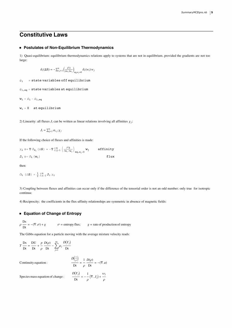
ü Postulates of Non-Equilibrium Thermodynamics
1) Quasi-equilibrium: equilibrium thermodynamics relations apply to systems that are not in equilibrium, provided the gradients are not toolarge;
∂t HDSL = -⁄i, j=1n J ∂2S
∂wi ∂w jNeq,wi=0
∂t HwiL w j
yi = state variables off equilibrium
yi,eq = state variables at equilibrium
wi = yi - yi,eq
wi = 0 at equilibrium
2) Linearity: all fluxes Ji can be written as linear relations involving all affinities c j;
Ji = ⁄j=1n ai, j c j
If the following choice of fluxes and affinities is made:
ci := T ∂wi HDSL = -T ⁄j=1n J ∂2S
∂wi ∂wjNeq,wi=0
wj affinity
Ji := ∂tHwiL flux
then:
∂t HDSL = 1T
⁄i=1n Ji ci
3) Coupling between fluxes and affinities can occur only if the difference of the tensorial order is not an odd number; only true for isotropiccontinua;
4) Reciprocity; the coefficients in the flux-affinity relationships are symmetric in absence of magnetic fields:
ü Equation of Change of Entropy
r Ds
Dt= -H“ .sL + g s = entropy flux; g = rate of production of entropy
The Gibbs equation for a particle moving with the average mixture velocity reads:
T Ds
Dt=
DU
Dt+p
r DHrLDt
-‚j=1
ns
m j DIY jM
Dt
Continuity equation :DJ 1
rN
Dt=
1
r DHrLDt
= -H“ .uL
Species mass equation of change :DIY jM
Dt= -
1
r I“ . J jM +
w j
r
SummaryMCEqns.nb 5

Internal energy equation of change :DU
Dt= -
1
r H“ .Hq+ qradLL -
p
r H“ . uL -
1
r Ht : “uL +‚
j=1
ns
IJ j. X jM
X j = external body forces
with the rate of production ê consumption of the j - th species : w j := ‚k=1
nr
Dn j,k rk
Substituting the substantial derivatives from the equation of continuity, species and internal energy conservation yields:
the entropy flux :
s =1
T Hq+ qradL -‚
j=1
ns
n j m j V j
the rate of production of entropy :
g = -1
T2 HHq+ qradL.“TL -‚
j=1
ns
n j V j. “m j
T-
1
T X j -
1
T Ht : “uL -
1
T ‚j=1
ns
m j w j
which indeed has the form :
∂t HDSL =1
T ‚i=1
n
Ji ci
ü Flux of Entropy
Define e as:
e := q+ qR -‚j=1
ns
n j H j V j
then:
s =e
T+‚
j=1
ns
n j S j V j
ü Rate of Entropy production
1. Define the "affinity" of k-th reaction:
Ak := -‚j=1
ns
m j Dn j,k
-1
T ‚j=1
ns
m j w j = +1
T ‚k=1
nr
rk Ak
The "affinity" the k-th reaction is in equilibrium if Ak is zero; if Ak is non zero then the reaction in in nonequilibrium, its net rate rk becomesnon zero and drives the state towards equilibrium.
2. Definedj as :
dj =nj
n K T Vsj -
mj
r “p + ‚
k=1,k≠j
ns ∂mj
∂xk p,T,xkHk≠jL “ck - Xj -
mj
r ‚k=1
ns
nk Xk
ck : molar fraction of k - th species
p = n K T ; for a perfect gas only
6 SummaryMCEqns.nb
mj nj = rj
Vsj =∂mj
∂p T,xkHk≠jL
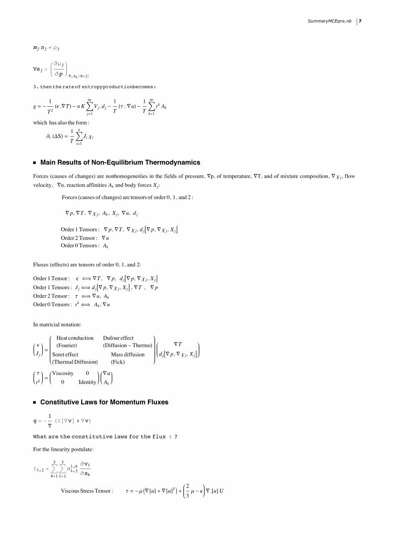
3. thenthe rateof entropyproductionbecomes:
g = -1
T2 He .“TL - n K ‚
j=1
ns
V j. d j -1
T Ht : “uL -
1
T ‚k=1
nr
rk Ak
which has also the form :
∂t HDSL =1
T ‚i=1
n
Ji ci
ü Main Results of Non-Equilibrium Thermodynamics
Forces (causes of changes) are nonhomogeneities in the fields of pressure, “p, of temperature, “T, and of mixture composition, “ c j, flowvelocity, “u, reaction affinities Ak and body forces X j:
Forces Hcauses of changesL are tensors of order 0, 1, and 2 :
“ p, “T , “ c j, Ak, X j, “u, d j
Order 1 Tensors : “ p, “T , “ c j, d jA“ p, “ c j, X jEOrder 2 Tensor : “uOrder 0 Tensors : Ak
Fluxes (effects) are tensors of order 0, 1, and 2:
Order 1 Tensor : e ó “T , “ p, d jA“ p, “ c j, X jEOrder 1 Tensors : J j ó d jA“ p, “ c j, X jE , “T , “ pOrder 2 Tensor : t ó “u, AkOrder 0 Tensors : rk ó Ak, “u
In matricial notation:
e
J j=
Heat conductionHFourierL
Dufour effectHDiffusion - ThermoL
Soret effectHThermal DiffusionL
Mass diffusionHFickL
“T
d jA“ p, “ c j, X jE
t
rk=
Viscosity 00 Identity
“uAk
ü Constitutive Laws for Momentum Fluxes
g = -1
T Ht@“vD : “vL
What are the constitutive laws for the flux t ?
For the linearity postulate:
ti,j = ‚k=1
3
‚l=1
3
ai,jl,k
∂vl
∂xk
Viscous Stress Tensor : t = - m I“@uD + “@uDTM +2
3 m - k “ .@uD U
SummaryMCEqns.nb 7
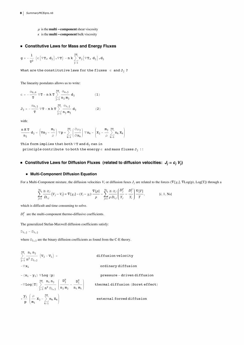
m is the multi -component shear viscosityk is the multi -component bulk viscosity
ü Constitutive Laws for Mass and Energy Fluxes
g = -1
T2 IeA“T, djE.“TM - n k ‚
j=1
ns
VjA“T, djE.dj
What are the constitutive laws for the fluxes e and Jj ?
The linearity postulates allows us to write:
e = -a0,0
T “T - n k T ‚
j=1
ns ao,j
nj mj dj H1L
Jj = -a0,j
T “T - n k T ‚
j=1
ns ai,j
nj mj dj H2L
with:
n K T
nj dj = Vsj -
mj
r “p + ‚
k=1
ns ∂mj
∂xk “xk - Xj -
mj
r ‚k=1
ns
nk Xk
This form implies that both “T and dj can in
principle contribute to both the energy e and mass fluxes Jj !!
ü Constitutive Laws for Diffusion Fluxes (related to diffusion velocities: Jj = cj Vj)
ü Multi-Component Diffusion Equation
For a Multi-Component mixture, the diffusion velocities Vi or diffusion fuxes J j are related to the forces (“@ciD, “Log(p), Log[T]) through aset of Ns PDEs:
‚j=1
Ns ci c j
Di, j IV j - ViM = “@ciD - HYi - ciL
“@pDp
-‚j=1
Ns ci c j
rDi, j D jT
Y j-DiT
Yi “@TDT
, 8i, 1, Ns<
which is difficult and time consuming to solve.
DiT are the multi-component thermo-diffusive coefficients.
The generalized Stefan-Maxwell diffusion coefficients satisfy:
i,j ~ i,j
where i,j are the binary diffusion coefficients as found from the C-E theory.
‚j=1
ns ni nj
n2 i,j IVj - ViM = diffusion velocity
-“xi ordinary diffusion
-Hxi - yiL “Log HpL pressure - driven diffusion
-“Log@TD ‚j=1
ns ni nj
n2 i,j
DjT
nj mj-
DiT
ni mithermal diffusion HSoret effectL
+yi
p
r
mi Xj - ‚
k=1
ns
nk Xk external forced diffusion
8 SummaryMCEqns.nb
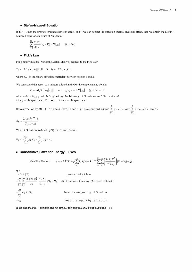
ü Stefan-Maxwell Equation
If Yi = ci then the pressure gradients have no effect, and if we can neglect the diffusion-thermal (Dufour) effect, then we obtain the Stefan-Maxwell eqns for a mixture of Ns species.
‚j=1
Ns ci c j
i, j IV j - ViM = “@ciD 8i, 1, Ns<
ü Fick's Law
For a binary mixture (Ns=2) the Stefan-Maxwell reduces to the Fick Law:
V1 = -1,2 “@Log@c1DD or J1 = -1,2 “@c1D
where 1,2 is the binary diffusion coefficient between species 1 and 2.
We can extend this result to a mixture diluted in the Ns-th component and obtain:
V j = - j “ALogAc jEE or c j V j = - j “Ac jE 8 j, 1, Ns - 1<where j º j,N , with j,N being the binary diffusion coefficients ofthe j - th species diluted in the N - th species.
However, only HN - 1L of the i are linearly independent since‚i=1
N
ci = 1, and‚i=1
N
ci Vi = 0; thus :
N =⁄j≠Nj “cj
⁄j≠N “cj
The diffusion velocity VN* is found from :
VN = -‚i=1
N-1
ci Vj = ‚i=1
N-1
i “ci
ü Constitutive Laws for Energy Fluxes
Heat Flux Vector : q = - k“@TD + r ‚i=1
Ns
hi Yi Vi + Ru T ‚i=1
Ns
‚j=1
Ns ci c j DiT
Wii, j IVi - V jM - qR
q =- k “@TD heat conduction
-‚i=1
ns
‚j=1
ns n K T DiT
ri xi xj
i,j IVj - ViM diffusive - thermo HDufour effectL
+‚j=1
ns
nj Hj Vj heat transport by diffusion
-qR heat transport by radiation
k is the multi - component thermal conductivity coefficient !!!
SummaryMCEqns.nb 9
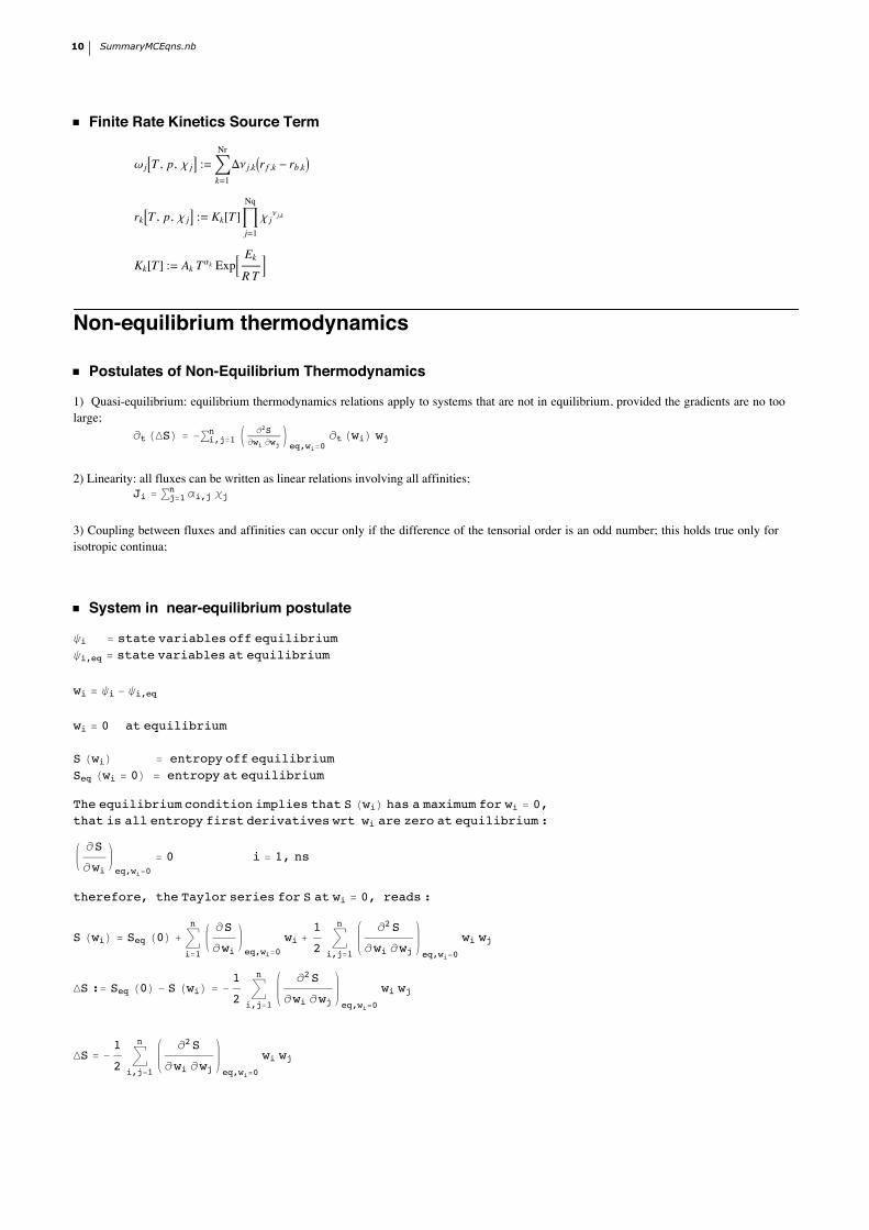
ü Finite Rate Kinetics Source Term
w jAT , p, c jE := ‚k=1
Nr
Dn j,kIr f ,k - rb,kM
rkAT , p, c jE := Kk@TD ‰j=1
Nq
c jn j,k
Kk@TD := Ak Tak ExpB EkR T
F
Non-equilibrium thermodynamics
ü Postulates of Non-Equilibrium Thermodynamics
1) Quasi-equilibrium: equilibrium thermodynamics relations apply to systems that are not in equilibrium, provided the gradients are no toolarge;
∂tHDSL = -⁄i,j=1n J ∂2S
∂wi ∂wjNeq,wi=0
∂tHwiL wj
2) Linearity: all fluxes can be written as linear relations involving all affinities; Ji = ⁄j=1
n ai,j cj
3) Coupling between fluxes and affinities can occur only if the difference of the tensorial order is an odd number; this holds true only forisotropic continua;
4) Reciprocity: the coefficients in the flux-affinity relationships are symmetric in absence of magnetic fields;
ü System in near-equilibrium postulate
yi = state variables off equilibriumyi,eq = state variables at equilibrium
wi = yi - yi,eq
wi = 0 at equilibrium
S HwiL = entropy off equilibriumSeq Hwi = 0L = entropy at equilibrium
The equilibrium condition implies that S HwiL has a maximum for wi = 0,that is all entropy first derivatives wrt wi are zero at equilibrium :
∂S
∂wi eq,wi=0
= 0 i = 1, ns
therefore, the Taylor series for S at wi = 0, reads :
S HwiL = Seq H0L + ‚i=1
n ∂S
∂wi eq,wi=0
wi +1
2 ‚i,j=1
n ∂2S
∂wi ∂wj eq,wi=0
wi wj
DS := Seq H0L - S HwiL = -1
2 ‚i,j=1
n ∂2S
∂wi ∂wj eq,wi=0
wi wj
DS = -1
2 ‚i,j=1
n ∂2S
∂wi ∂wj eq,wi=0
wi wj
10 SummaryMCEqns.nb
DS = - ‚i,j=1
n
eq,wi=0
wi wj
∂tHDSL = - ‚i,j=1
n ∂2S
∂wi ∂wj eq,wi=0
∂tHwiL wj
ü Linearity Postulate
Linear Relation between fluxes Ji and affinities cj is postulated(small departures from equilibrium)
Ji = ‚j=1
n
ai,j cj
ai,j direct HdiagonalL couplingsai,j off diagonal couplings
ü Onsager postulate (reciprocity)
The coefficients in the flux-affinity relationships are symmetric in absence of magnetic fields
ai,j = aj,i
What is the optimal choice for fluxes and affinities,so that the Onsager principle will hold ?
If the following choice of fluxes and affinities is made:
ci := T ∂wi HDSL = -T ‚j=1
n ∂2S
∂wi ∂wj eq,wi=0
wj affinity
Ji := ∂tHwiL flux
then:
∂t HDSL =1
T ‚i=1
n
Ji ci
ü Equation of Change of Entropy
r Ds
Dt= -H“.sL + g
Continuity equation :D I 1
rM
Dt=1
r D HrLDt
= -I“.vèM
Species mass equation of change :D IyjMDt
= -1
r I“.JjM +
wj
r
Internal energy equation of change :DU
Dt= -
1
r H“.Hq + qRLL -
p
r I“.vèM -
1
r It : “vèM + ‚
j=1
ns
IJj. XjM
Xj = external body forces
with the rate of productionêconsumption of j - th species : wj := ‚k=1
nr
Dnj,k rk
The Gibbs equation for a particle moving with the average mixture velocity reads:
T Ds
Dt=DU
Dt+p
r D HrLDt
- ‚j=1
ns
mj D IyjMDt
Substituting the substantial derivatives from the equation of continuity, species and internal energy conservation yields:
SummaryMCEqns.nb 11
Substituting the substantial derivatives from the equation of continuity, species and internal energy conservation yields:
the entropy flux :
s =1
T Hq + qRL - ‚
j=1
ns
nj mj Vj
the rate of production of entropy :
g = -1
T2 HHq + qRL.“TL - ‚
j=1
ns
nj Vj. “mj
T-1
T Xj -
1
T Ht : “vL -
1
T ‚j=1
ns
mj wj
ü Flux of Entropy
Define e as:
e := q + qR - ‚j=1
ns
nj Hj Vj
then:
s =1
T Hq + qRL - ‚
j=1
ns
nj mj Vj
s =1
T e + ‚
j=1
ns
nj Hj Vj - ‚j=1
ns
nj IHj - T SjM Vj
and finally
s =e
T+ ‚j=1
ns
nj Sj Vj
ü Rate of Entropy production
g = -1
T2 HHq + qRL.“TL - ‚
j=1
ns
nj Vj. “mj
T-1
T Xj -
1
T Ht : “vL -
1
T ‚j=1
ns
mj wj
The contribution to entropy production due to gradients of chemical potentials, temperature and external forces is:
g = -1
T2 HHq + qRL.“TL - ‚
j=1
ns
nj Vj. “mj
T-1
T Xj
g = -1
T2 HHq + qRL.“TL -
1
T ‚j=1
ns
nj Vj. T “mj
T- Xj
g = -1
T2 HHq + qRL.“TL -
1
T ‚j=1
ns
nj Vj. T “mj
T+1
T ‚j=1
ns
nj Vj.Xj
---------------------------------------
T “mj
T= T
“mj
T-
mj
T “T
T= “mj - mj
“T
T= “mj - IHj - T SjM
“T
T= “mj - Hj
“T
T+ T Sj
“T
T
“mj =∂mj
∂p T,xk Hk≠jL “p +
∂mj
∂T p,xk Hk≠jL “T + ‚
k=1,k≠j
ns ∂mj
∂xk p,T,xk Hk≠jL “xk
Vsj =∂mj
∂p T,xk Hk≠jL
12 SummaryMCEqns.nb

Sj = -∂mj
∂T p,xk Hk≠jL
“mj = Vsj “p - Sj “T + ‚k=1,k≠j
ns ∂mj
∂xk p,T,xk Hk≠jL “xk
T “mj
T= Vsj “p - Sj “T + ‚
k=1,k≠j
ns ∂mj
∂xk p,T,xk Hk≠jL “xk -
Hj
T “T + Sj “T
---------------------------------------
g = -1
T2 e + ‚
j=1
ns
nj Hj Vj .“T -
1
T ‚j=1
ns
nj Vj. Vsj “p - Sj “T + ‚k=1,k≠j
ns ∂mj
∂xk p,T,xk Hk≠jL “xk -
Hj
T “T + Sj “T +
1
T ‚j=1
ns
nj Vj.Xj
g = -1
T2 He.“TL -
1
T2 ‚j=1
ns
nj Hj Vj.“T -1
T ‚j=1
ns
nj Vj.Vsj “p -
1
T ‚j=1
ns
nj Vj. ‚k=1,k≠j
ns ∂mj
∂xk p,T,xk Hk≠jL “xk +
1
T ‚j=1
ns
nj Vj.Hj
T “T +
1
T ‚j=1
ns
nj Vj.Xj
g = -1
T2 He.“TL -
1
T ‚j=1
ns
nj Vj.Vsj “p -1
T ‚j=1
ns
nj Vj. ‚k=1,k≠j
ns ∂mj
∂xk p,T,xk Hk≠jL “xk +
1
T ‚j=1
ns
nj Vj.Xj
Jj = mj nj Vj = rj Vj
g = -1
T2 He.“TL -
1
T ‚j=1
ns
nj Jj.:Vsj
mj “p +
1
mj ‚k=1,k≠j
ns ∂mj
∂xk p,T,xk Hk≠jL “xk -
Xj
mj>
---------------------------------------
Define Lj as :
Lj :=Vsj
mj “p +
1
mj ‚k=1,k≠j
ns ∂mj
∂xk p,T,xk Hk≠jL “xk -
Xj
mj
so that:
g = -1
T2 He.“TL -
1
T ‚j=1
ns
nj Jj.Lj
---------------------------------------
Define dj as :
dj :=nj mj
n K T Lj -
1
r “p +
1
r ‚k=1
ns
nk Xk
substitute Lj in dj to have :
dj =nj
n K T
mj Vsj
mj-mj
r “p +
mj
mj ‚k=1,k≠j
ns ∂mj
∂xk p,T,xk Hk≠jL “xk -
mj Xj
mj-mj
r ‚k=1
ns
nk Xk
n K T
nj dj = Vsj -
mj
r “p + ‚
k=1,k≠j
ns ∂mj
∂xk p,T,xk Hk≠jL “xk - Xj -
mj
r ‚k=1
ns
nk Xk
introducing the definition of the diffusional forces dj in g yields :
SummaryMCEqns.nb 13

g = -1
T2 He.“TL -
1
T ‚j=1
ns
nj Jj.Lj =
= -1
T2 He.“TL - n K ‚
j=1
ns
Vj.dj
---------------------------------------
If we define
Ak := -‚j=1
ns
mj Dnj,k
as the "affinity" of k-th reaction, then the contribution to the entropy production due to chemical reactions is:
-1
T ‚j=1
ns
mj wj = +1
T ‚k=1
nr
rk Ak
---------------------------------------
g = -1
T2 He.“TL - n K ‚
j=1
ns
Vj.dj -1
T Ht : “vL -
1
T ‚k=1
nr
rk Ak
ü Rate of Entropy production as inner product between fluxes and affinities
∂t HDSL =1
T ‚i=1
n
Ji ci
g = -1
T2 He.“TL - n K ‚
j=1
ns
Vj.dj -1
T Ht : “vL -
1
T ‚k=1
nr
rk Ak
It follows that :
∂t HDSL ~ g
Curie's postulate insures that coupling might occur only betweentensors whose order differs by an odd number,that is:
Order 1 Tensors : e ó “T, djA“p, “xj, XjEOrder 1 Tensors : Jj ó djA“p, “xj, XjE , “T
Order 2 Tensors : t ó “v, AkOrder 0 Tensors : rk ó Ak, “v
or in matricial notation:
e
Jj=
Heat conduction Dufour effectHdiffusion - thermoL
Soret effectHthermal diffusionL
Mass diffusion
“T
djA“p, “xj, XjE
t
rk=
Viscosity 00 Identity
K“vAk
O
ü Constitutive Laws for the Momentum Flux
g = -1
T Ht : “vL
For the linearity postulate:
14 SummaryMCEqns.nb

ti,j = ‚k=1
3
‚l=1
3
ai,jl,k
∂vl
∂xk
For the Onsager principle:
ai,jl,k = al,k
i,j
Since the pressure tensor is symmetric, then:
ai,jl,k = aj,i
l,k
Combining the two properties yields:
ai,jl,k = ai,j
k,l
Therefore:
ti,j = -1
2 ‚k=1
3
‚l=1
3
ai,jl,k
∂vl
∂xk+
∂vk
∂xl
where only 21 ai,jl,k are independent, and are the elastic constants of the continuum medium.
If the medium is isotropic then the stress-strain relationship is indipendent of rotations of the reference frame, and there are only 2 independentconstants, that is m, the shear viscosity, and k, the bulk viscosity:
t = -m I“v + H“vLTM +2
3 m - k H“.vL U = -2 m S
where:
S =1
2 :I“v + H“vLTM -
2
3 m - k H“.vL U>
The shear and bulk (?) viscosity coefficients are found from the C-E theory
This is the linear stress-strain relationship adopted in the Navier-Stokes equations.
By replacing this last expression in g yields:
g = -1
T H-2 m S : “vL
g =2 m
T HS : SL +
k
T H“.vL2
where:
S =1
2 :I“v + H“vLTM +
2
3 m - k H“.vL U>
Since g r 0 for the 2 - nd principle of thermodynamics, and HS : SL r 0, H“.vL2 r 0, it follows that :
m, k r0
ü Constitutive Laws for the Chemical Reactions Flux
g = -1
T ‚k=1
nr
rk Ak
rk = rfk - rb
k = Kfk HTL ‰
j=1
ns
cj,kn' - Kb
k HTL ‰j=1
ns
cj,kn''
SummaryMCEqns.nb 15
ü Constitutive Laws for the Energy and Mass Fluxes
g = -1
T2 He.“TL - n k ‚
j=1
ns
Vj.dj
What are the constitutive laws for the fluxes e and Jj ?
The linearity postulates allows us to write:
e = -a0,0
T “T - n k T ‚
j=1
ns ao,j
nj mj dj H1L
Jj = -a0,j
T “T - n k T ‚
j=1
ns ai,j
nj mj dj H2L
with:
n K T
nj dj = Vsj -
mj
r “p + ‚
k=1
ns ∂mj
∂xk “xk - Xj -
mj
r ‚k=1
ns
nk Xk
This form implies that both “T and dj can in
principle contribute to both the energy e and mass fluxes Jj !!
---------------------------------------
For a perfect gas
p = n K T
mj = mj,0 HTL + k T LogAp xjE = mj,0 HTL + k T Log@p D + k T LogAxjEwhich implies:
Vsj =∂mj
∂p=k T
p=1
n;
∂mj
∂xj p,T,xk Hk≠jL=k T
xj;
∂mj
∂xk= 0
that is, the diffusional forces can be cast as:
n K T dj =nj
n-nj mj
r “p + n k T “xj -
nj mj
r
r
mj Xj - ‚
k=1
ns
nk Xk
dj = “xj + Ixj - yjM “Log HpL -yj
p
r
mj Xj - ‚
k=1
ns
nk Xk
---------------------------------------
From the C-E kinetic theory of diluted gases:
e = -l' “T - n k T ‚j=1
ns DjT
nj mj dj H3L
Jj = -DjT
T “T -
n2
r‚j=1
ns
mi mj i,j dj H4L
where, the coefficient l' is found from the C-E theory.
These are the generalized Fick equations for the mass fluxes.In matrix form they read:
@JD = @D “B Tdj
F
---------------------------------------
16 SummaryMCEqns.nb

---------------------------------------
Comparing (1-2) with (3-4) yields:
l' =a0,0
T
Multi -component thermal -diffusion coefficients: DjT = ao,j = aj,o
Multi -component Fick diffusivities: i,j =r K T
n mi mj
ai,j
nj mj+
1
ni mi ‚k=1,k≠j
ns
ai,k
Solving the generalized Fick equation wrt “B Tdj
F yields:
“B Tdj
F = -@D-1@JD
that is:
di = ‚j=1
ns ni nj
n2 i,j
DjT
nj mj-
DiT
ni mi “Log@TD + ‚
j=1
ns ni nj
n2 i,j IVj - ViM
These are the (ns-1) generalized Stefan-Maxwell equations.
Multi-component Stefan-Maxwell diffusivities: i,j = Ii,jMThe generalized Stefan-Maxwell diffusion coefficients satisfy:
i,j ~ i,j
where i,j are the binary diffusion coefficients as found from the C-E theory.
---------------------------------------
For a binary mixture, the generalized Stefan-Maxwell equations reduce to :
n2 1,2
n1 n2 Hd1 + kT “Log@TDL = V2 - V1
with kT :
kT :=r
n2 m1 m2 D1T
1,2
referred to as the thermal-diffusion ratio coefficient.
ü Returning to the mass fluxes (diffusion velocities):
By replacing the definition of di for diluted ideal gases in the generalized Stefan-Maxwell equation yields an equation for the diffusionvelocities in terms of state variables gradients:
‚j=1
ns ni nj
n2 i,j IVj - ViM = diffusion velocity
-“xi ordinary diffusion
-Hxi - yiL “Log HpL pressure - driven diffusion
-“Log@TD ‚j=1
ns ni nj
n2 i,j
DjT
nj mj-
DiT
ni mithermal diffusion HSoret effectL
+yi
p
r
mi Xj - ‚
k=1
ns
nk Xk external forced diffusion
---------------------------------------
SummaryMCEqns.nb 17
---------------------------------------
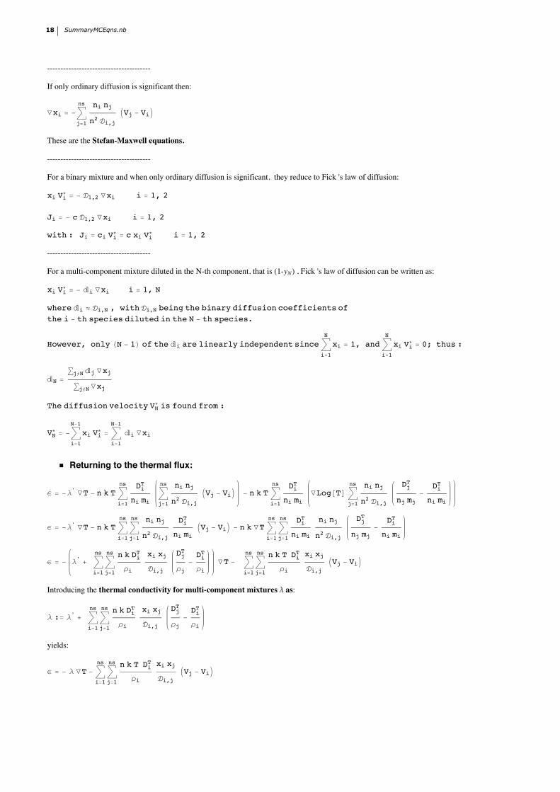
If only ordinary diffusion is significant then:
“xi = -‚j=1
ns ni nj
n2 i,j IVj - ViM
These are the Stefan-Maxwell equations.
---------------------------------------
For a binary mixture and when only ordinary diffusion is significant, they reduce to Fick 's law of diffusion:
xi Vi* = - 1,2 “xi i = 1, 2
Ji = - c 1,2 “xi i = 1, 2
with : Ji = ci Vi* = c xi Vi
* i = 1, 2
---------------------------------------
For a multi-component mixture diluted in the N-th component, that is (1-yN) , Fick 's law of diffusion can be written as:
xi Vi* = - i “xi i = 1, N
where i º i,N , with i,N being the binary diffusion coefficients ofthe i - th species diluted in the N - th species.
However, only HN - 1L of the i are linearly independent since‚i=1
N
xi = 1, and‚i=1
N
xi Vi* = 0; thus :
N =⁄j≠Nj “xj
⁄j≠N “xj
The diffusion velocity VN* is found from :
VN* = -‚
i=1
N-1
xi Vi* = ‚
i=1
N-1
i “xi
ü Returning to the thermal flux:
e = -l' “T - n k T ‚i=1
ns DiT
ni mi ‚
j=1
ns ni nj
n2 i,j IVj - ViM - n k T ‚
i=1
ns DiT
ni mi “Log@TD ‚
j=1
ns ni nj
n2 i,j
DjT
nj mj-
DiT
ni mi
e = -l' “T - n k T ‚i=1
ns
‚j=1
ns ni nj
n2 i,j DiT
ni mi IVj - ViM - n k “T ‚
i=1
ns
‚j=1
ns DiT
ni mi ni nj
n2 i,j
DjT
nj mj-
DiT
ni mi
e = - l' + ‚i=1
ns
‚j=1
ns n k DiT
ri xi xj
i,j DjT
rj-DiT
ri “T - ‚
i=1
ns
‚j=1
ns n k T DiT
ri xi xj
i,j IVj - ViM
Introducing the thermal conductivity for multi-component mixtures l as:
l := l' + ‚i=1
ns
‚j=1
ns n k DiT
ri xi xj
i,j DjT
rj-DiT
ri
yields:
e = - l “T - ‚i=1
ns
‚j=1
ns n k T DiT
ri xi xj
i,j IVj - ViM
18 SummaryMCEqns.nb
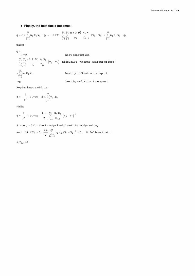
ü Finally, the heat flux q becomes:
q = e + ‚j=1
ns
nj Hj Vj - qR = - l “T - ‚i=1
ns
‚j=1
ns n k T DiT
ri xi xj
i,j IVj - ViM + ‚
j=1
ns
nj Hj Vj - qR
that is:
q =- l “T heat conduction
-‚i=1
ns
‚j=1
ns n k T DiT
ri xi xj
i,j IVj - ViM diffusive - thermo HDufour effectL
+‚j=1
ns
nj Hj Vj heat by diffusion transport
-qR heat by radiation transport
Replacing e and dj in :
g = -1
T2 He.“TL - n k ‚
j=1
ns
Vj.dj
yields:
g =l
T2 H“T.“TL -
k n
2 ‚i,j=1
ns xi xj
i,j IVj - ViM2
Since g r 0 for the 2 - nd principle of thermodynamics,
and H“T.“TL r 0,k n
2 ‚i,j=1
ns
xi xj IVj - ViM2 r 0, it follows that :
l, i,j r0
SummaryMCEqns.nb 19