Indefinite Zeta Functions

Gene S. Kopp

University of Bristol

Vanderbilt University Number Theory Seminar

September 22, 2020

1

Outline

Part One: Hilbert’s 12th ProblemMy personal motivation for this work

Part Two and Three: Indefinite Theta and Indefinite ZetaA general construction with potential applications beyond the

motivating problem

Part Four: Kronecker Limit FormulasAn application of the general construction to one aspect of the

motivating problem

2

Part One: Hilbert’s 12th Problem

3

Hilbert’s 12th problem

List of 23 open problems published in 190012th problem asks for an “Extension ofKronecker’s Theorem on Abelian Fields toany Algebraic Realm of Rationality.”Kronecker’s Theorem (Kronecker-Webertheorem) says that the abelian extensions ofQ are generated by the values ofe(z) = e2πiz at rational values of z.Given any base field (“realm of rationality”),Hilbert wanted “analytic functions” that playthe role of e(z).

4

Class field theory

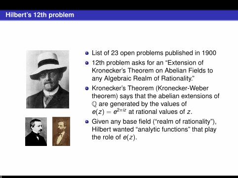
The imaginary quadratic case was mostly known to Hilbert anduses the theory of elliptic curves with complex multiplication(CM), due to Weber and others.Abstract class field theory, developed during the 1910s and1920s by Takagi and others, constructs class fields in an indirectmanner.

Goro Shimura generalized CM theory to“CM base fields” by replacing elliptic curveswith abelian varieties.

5

Stark conjectures

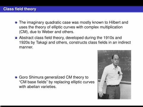
Introduced 1971–1980 by Harold StarkArtin L-function L(s, ρ) for irrepρ : Gal(L/K )→ GLn(C)

Taylor series at s = 0: L(s, ρ) = cr sr + · · ·

Leading coefficient cr conjectured to be a product of an algebraicnumber and a “Stark regulator”, a determinant of an r × r matrixof linear forms of logarithms of algebraic units.If L/K is an abelian, L(s, ρ) = L(s, χ) is a HeckeL-function—specified by data internal to K .Units are predicted to live in the corresponding class field.Partial answer to Hilbert’s 12th problem in the “rank 1” case(r = 1), when we can recover the Stark units by exponentiation.The rank 1 abelian Stark conjectures remain open for any realquadratic field, e.g., Q(

√3).

6

L-functions at s = 1: rational example

This formula can be proved using calculus. Try it! Hint: Replace 1n

with xn

n and take a derivative.

Example

1− 13− 1

5+

17

+19− 1

11− 1

13+

115

+−−+ · · · =1√2

log(

1 +√

2)

The left-hand side is the value L(1, χ), where χ(n) =( 2

n

)is the

Dirichlet character associated to the field extension Q(√

2)/Q. Theright-hand side involves ε = 1 +

√2, the fundamental unit of Q(

√2).

7

L-functions at s = 1: imaginary quadratic example

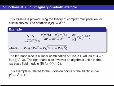
This formula is proved using the theory of complex multiplication forelliptic curves. The notation e(z) := e2πiz .

Example ∑∑(m,n)∈Z2\(0,0)

e(m/5)− e(2m/5)

m2 + mn + n2 =2π√

3log(ε1/5

)

where ε = 29 + 12√

5 + 2√

6(65 + 29√

5).

The left-hand side is a linear combination of Hecke L-values at s = 1for Q(

√−3). The right-hand side involves an algebraic unit ε in the

ray class field modulo (5) for Q(√−3).

This example is related to the 5-torsion points of the elliptic curvey2 = x3 + 1.

8

L-functions at s = 1: real quadratic example

This formula is an open conjecture!

Example∞∑

m=1

∑n∈Z

− 53 m≤n< 5

3 m

e (4m/5)− e (m/5)

3m2 − n2 =π

i√

3log (ε) ,

where ε ≈ 3.890861714 is a root of the polynomial equation

x8 − (8 + 5√

3)x7 + (53 + 30√

3)x6 − (156 + 90√

3)x5

+ (225 + 130√

3)x4 − (156 + 90√

3)x3 + (53 + 30√

3)x2

− (8 + 5√

3)x + 1 = 0.

The number ε is an algebraic unit in the narrow ray class field ofQ(√

3) modulo 5.

9

Kronecker limit formulas

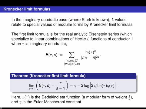
In the imaginary quadratic case (where Stark is known), L-valuesrelate to special values of modular forms by Kronecker limit formulas.

The first limit formula is for the real analytic Eisenstein series (whichspecialize to linear combinations of Hecke L-functions of conductor 1when τ is imaginary quadratic),

E(τ, s) :=∑

(m,n)∈Z2

(m,n) 6=(0,0)

Im(τ)s

|mτ + n|2s .

Theorem (Kronecker first limit formula)

lims→1

(E(τ, s)− π

s − 1

)= γ − 2 log

∣∣∣2√Im(τ)η(τ)∣∣∣ .

Here, η(τ) is the Dedekind eta function (a modular form of weight 12 ),

and γ is the Euler-Mascheroni constant.10

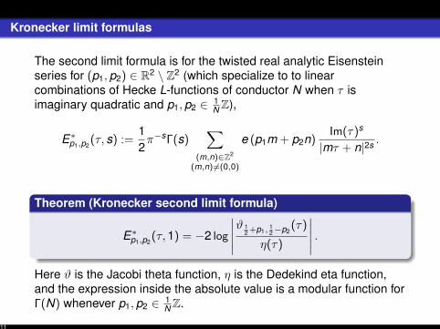
Kronecker limit formulas

The second limit formula is for the twisted real analytic Eisensteinseries for (p1,p2) ∈ R2 \ Z2 (which specialize to to linearcombinations of Hecke L-functions of conductor N when τ isimaginary quadratic and p1,p2 ∈ 1

N Z),

E∗p1,p2(τ, s) :=

12π−sΓ(s)

∑(m,n)∈Z2

(m,n) 6=(0,0)

e (p1m + p2n)Im(τ)s

|mτ + n|2s .

Theorem (Kronecker second limit formula)

E∗p1,p2(τ,1) = −2 log

∣∣∣∣∣ϑ 12 +p1,

12−p2

(τ)

η(τ)

∣∣∣∣∣ .Here ϑ is the Jacobi theta function, η is the Dedekind eta function,and the expression inside the absolute value is a modular function forΓ(N) whenever p1,p2 ∈ 1

N Z.

11

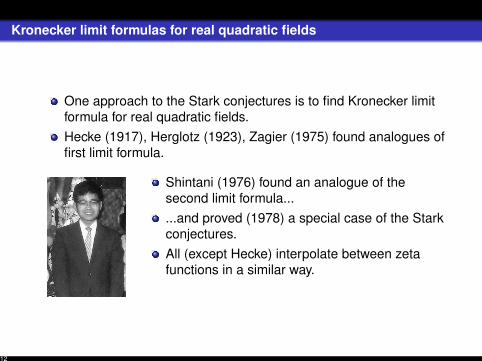
Kronecker limit formulas for real quadratic fields

One approach to the Stark conjectures is to find Kronecker limitformula for real quadratic fields.Hecke (1917), Herglotz (1923), Zagier (1975) found analogues offirst limit formula.

Shintani (1976) found an analogue of thesecond limit formula......and proved (1978) a special case of the Starkconjectures.All (except Hecke) interpolate between zetafunctions in a similar way.

12

Kronecker limit formulas for real quadratic fields

We introduce a new way of interpolating that preserves thefunctional equation......and obtain a new Kronecker limit formula (analogous tosecond).Gives a new, fast-converging analytic formula for (presumptive)Stark units......but does not (yet) help with proving algebraicity.

13

Part Two: Indefinite Theta Functions

14

Zwegers’s thesis

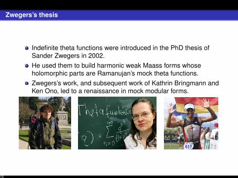
Indefinite theta functions were introduced in the PhD thesis ofSander Zwegers in 2002.He used them to build harmonic weak Maass forms whoseholomorphic parts are Ramanujan’s mock theta functions.Zwegers’s work, and subsequent work of Kathrin Bringmann andKen Ono, led to a renaissance in mock modular forms.

15

Generalizing Zwegers’s theta

Let M be a real symmetric matrix of signature (g − 1,1) andc1, c2 ∈ Rg satisfying c>j Acj < 0. Zwegers’s indefinite theta function isϑc1,c2

M (z, τ) for z ∈ Cg and τ ∈ H. We generalize it by...Replacing τM with a symmetric matrix Ω = N + iM such that Mhas signature (g − 1,1). Fairly straightforward.Allowing c1, c2 to take complex values. Not straightforward.To get a good transformation theory, the latter is required to oncewe do the former.

16

Siegel intermediate half-space

Definition (Siegel intermediate half-space)

For 0 ≤ k ≤ g, we define the Siegel intermediate half-space of genusg and index k to be

H(k)g = Ω ∈ Mg(C) : Ω = Ω> and Im(Ω) has signature (g − k , k).

17

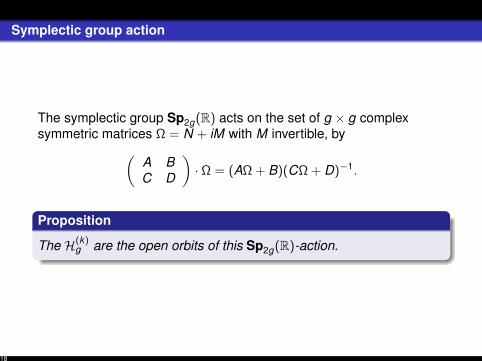
Symplectic group action

The symplectic group Sp2g(R) acts on the set of g × g complexsymmetric matrices Ω = N + iM with M invertible, by(

A BC D

)· Ω = (AΩ + B)(CΩ + D)−1.

Proposition

The H(k)g are the open orbits of this Sp2g(R)-action.

18

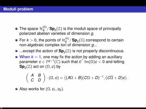
Moduli problem

The space H(0)g /Sp2(Z) is the moduli space of principally

polarized abelian varieties of dimension g.

For k > 0, the points of H(k)g /Sp2(Z) correspond to certain

non-algebraic complex tori of dimension g......except the action of Sp2(Z) is not properly discontinuous.When k = 1, one may fix the action by adding an auxiliaryparameter c ∈ Pg−1(C) such that c> Im(Ω)c < 0 and lettingSp2(Z) act on (Ω, c) by(

A BC D

)· (Ω, c) =

((AΩ + B)(CΩ + D)−1, (CΩ + D)c

).

Also works for (Ω, c1, c2).

19

Definition of definite (Riemann) theta function

This function was defined by Riemann and is known as the Riemanntheta function.

Definition (Definite theta function)

Let z ∈ Cg and Ω = N + iM ∈ H(0)g . Define

Θ(z; Ω) =∑n∈Zg

e(

12

n>Ωn + n>z).

The sum will only converge if the bilinear form QM(n) = 12 n>Mn is

positive definite—that is, if Ω ∈ H(0)g .

20

Definition of indefinite theta function

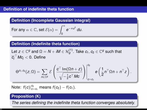
Definition (Incomplete Gaussian integral)

For any α ∈ C, set E(α) =

∫ α

0e−πu2

du.

Definition (Indefinite theta function)

Let z ∈ Cg and Ω = N + iM ∈ H(1)g . Take c1, c2 ∈ Cg such that

cj>Mcj < 0. Define

Θc1,c2 (z; Ω) =∑n∈Zg

E

c> Im(Ωn + z)√− 1

2 c>Mc

∣∣∣∣∣∣c2

c=c1

e(

12

n>Ωn + n>z).

Note: f (c)|c2c=c1

means f (c2)− f (c1).

Proposition (K)

The series defining the indefinite theta function converges absolutely.21

Theta functions with real characteristics

We switch to a different notation because it will make our formulasnicer.

Definition (Definite theta null with real characteristics)

For “characteristics” p,q ∈ Rg and Ω ∈ H(0)g , set

Θp,q(Ω) = e(

12

q>Ωq + p>q)

Θ (p + Ωq,Ω) .

Definition (Indefinite theta null with real characteristics)

For “characteristics” p,q ∈ Rg , Ω ∈ H(1)g , and c1, c2 ∈ Cg such that

cj> Im(Ω)cj < 0, set

Θc1,c2p,q (Ω) = e

(12

q>Ωq + p>q)

Θc1,c2 (p + Ωq; Ω) .

22

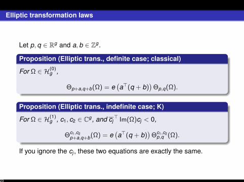
Elliptic transformation laws

Let p,q ∈ Rg and a,b ∈ Zg .

Proposition (Elliptic trans., definite case; classical)

For Ω ∈ H(0)g ,

Θp+a,q+b(Ω) = e(a>(q + b)

)Θp,q(Ω).

Proposition (Elliptic trans., indefinite case; K)

For Ω ∈ H(1)g , c1, c2 ∈ Cg , and cj

> Im(Ω)cj < 0,

Θc1,c2p+a,q+b(Ω) = e

(a>(q + b)

)Θc1,c2

p,q (Ω).

If you ignore the cj , these two equations are exactly the same.

23

Modular transformation laws, definite case

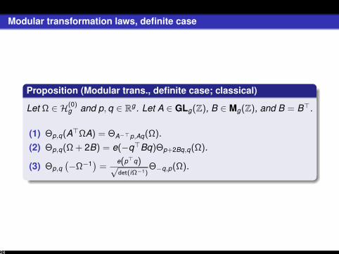
Proposition (Modular trans., definite case; classical)

Let Ω ∈ H(0)g and p,q ∈ Rg . Let A ∈ GLg(Z), B ∈ Mg(Z), and B = B>.

(1) Θp,q(A>ΩA) = ΘA−>p,Aq(Ω).(2) Θp,q(Ω + 2B) = e(−q>Bq)Θp+2Bq,q(Ω).

(3) Θp,q(−Ω−1

)=

e(p>q)√det(iΩ−1)

Θ−q,p(Ω).

24

Modular transformation laws, indefinite case

Theorem (Modular trans., indefinite case; K)

Let Ω = N + iM ∈ H(1)g , c1, c2 ∈ Cg such that cj

>Mcj < 0, andp,q ∈ Rg . Let A ∈ GLg(Z), B ∈ Mg(Z), and B = B>.

(1) Θc1,c2p,q (A>ΩA) = ΘAc1,Ac2

A−>p,Aq(Ω).

(2) Θc1,c2p,q (Ω + 2B) = e(−q>Bq)Θc1,c2

p+2Bq,q(Ω).

(3) Θc1,c2p,q (−Ω−1) = e(p>q)√

det(iΩ−1)Θ−Ω

−1c1,−Ω−1c2

−q,p (Ω).

The case when N is a constant multiple of M and c1, c2 ∈ Rg is due toZwegers. If you ignore the cj , these are exactly the same equationsas on the previous slide.

25

Part Three: Indefinite Zeta Functions

26

Definition of definite and indefinite zeta function

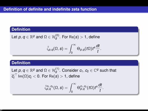
Definition

Let p,q ∈ Rg and Ω ∈ H(0)g . For Re(s) > 1, define

ζp,q(Ω, s) =

∫ ∞0

Θp,q(tΩ)ts dtt.

Definition

Let p,q ∈ Rg and Ω ∈ H(1)g . Consider c1, c2 ∈ Cg such that

cj> Im(Ω)cj < 0. For Re(s) > 1, define

ζc1,c2p,q (Ω, s) =

∫ ∞0

Θc1,c2p,q (tΩ)ts dt

t.

27

Analytic continuation and rapid convergence

Theorem (Analytic continuation; K)

For any choice of r > 0, the following expression is an analyticcontinuation of ζc1,c2

p,q (Ω, s) to the entire s-plane.

ζc1,c2p,q (Ω, s) =

∫ ∞r

Θc1,c2p,q (tΩ)ts dt

t

+e(p>q)√det(−iΩ)

∫ ∞r−1

ΘΩc1,Ωc2−q,p

(t(−Ω−1)) t

g2−s dt

t.

I have used this formula for computer calculations, as it may be usedto compute the indefinite zeta function to arbitrary precision inpolynomial time.

28

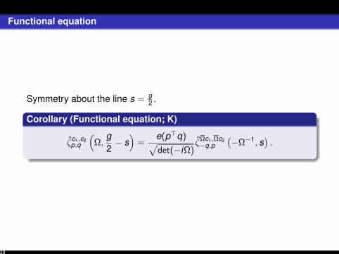
Functional equation

Symmetry about the line s = g2 .

Corollary (Functional equation; K)

ζc1,c2p,q

(Ω,

g2− s)

=e(p>q)√det(−iΩ)

ζΩc1,Ωc2−q,p

(−Ω−1, s

).

29

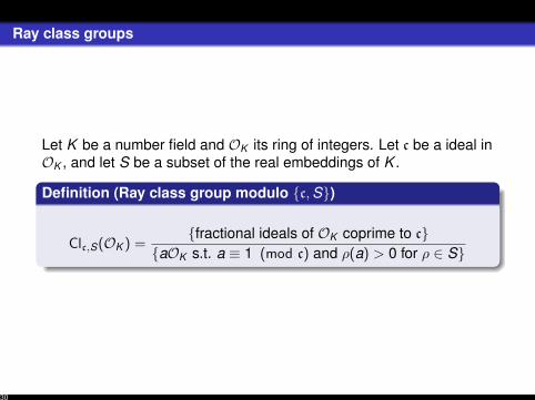
Ray class groups

Let K be a number field and OK its ring of integers. Let c be a ideal inOK , and let S be a subset of the real embeddings of K .

Definition (Ray class group modulo c,S)

Clc,S(OK ) =fractional ideals of OK coprime to c

aOK s.t. a ≡ 1 (mod c) and ρ(a) > 0 for ρ ∈ S

30

Zeta functions associated to ray classes

DefinitionFor A ∈ Clc,S(OK ), the associated zeta function is

ζ(s,A) =∑a≤OKa∈A

N(a)−s.

Let R ∈ Clc,S(OK ) be the ideal class

R = aOK : a ≡ −1 (mod c) and ρ(a) > 0 for ρ ∈ S.

DefinitionFor A ∈ Clc,S(OK ), the associated differenced zeta function is

ZA(s) = ζ(s,A)− ζ(s,RA).

31

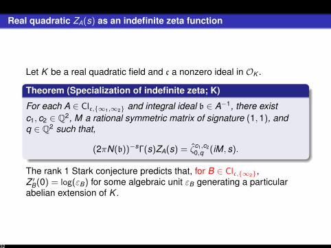
Real quadratic ZA(s) as an indefinite zeta function

Let K be a real quadratic field and c a nonzero ideal in OK .

Theorem (Specialization of indefinite zeta; K)

For each A ∈ Clc,∞1,∞2 and integral ideal b ∈ A−1, there existc1, c2 ∈ Q2, M a rational symmetric matrix of signature (1,1), andq ∈ Q2 such that,

(2πN(b))−sΓ(s)ZA(s) = ζc1,c20,q (iM, s).

The rank 1 Stark conjecture predicts that, for B ∈ Clc,∞2,Z ′B(0) = log(εB) for some algebraic unit εB generating a particularabelian extension of K .

32

Example

Let K = Q(√

3), so OK = Z[√

3], and let c = 5OK .The ray class group Clc,∞2

∼= Z/8Z. Let I be the identity.The ray class group Clc,∞1,∞2

∼= Z/2Z× Z/8Z. WriteI = I+ t I−, where I+ is the identity element of Clc,∞1,∞2.We have ZI(s) = ZI+ (s) + ZI−(s). But it turns out that ZI−(s) isidentically zero in this case, so ZI(s) = ZI+ (s).

For q = 15

(10

), c1 =

(01

), and P =

(2 31 2

),

Z ′I (0) = Z ′I+ (0)

= ζc1,P3c10,q (iM,0)

= ζc1,Pc10,q (iM,0) + ζPc1,P2c1

0,q (iM,0) + ζP2c1,P3c10,q (iM,0)

= ζc1,Pc10,q0

(iM,0) + ζc1,Pc10,q1

(iM,0) + ζc1,Pc10,q2

(iM,0),

where q0 = 15

(10

), q1 = 1

5

(21

), and q2 = 1

5

(24

).

33

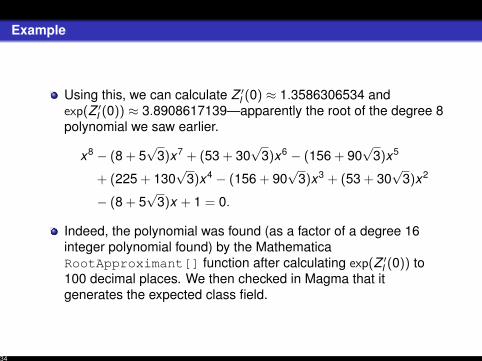
Example

Using this, we can calculate Z ′I (0) ≈ 1.3586306534 andexp(Z ′I (0)) ≈ 3.8908617139—apparently the root of the degree 8polynomial we saw earlier.

x8 − (8 + 5√

3)x7 + (53 + 30√

3)x6 − (156 + 90√

3)x5

+ (225 + 130√

3)x4 − (156 + 90√

3)x3 + (53 + 30√

3)x2

− (8 + 5√

3)x + 1 = 0.

Indeed, the polynomial was found (as a factor of a degree 16integer polynomial found) by the MathematicaRootApproximant[] function after calculating exp(Z ′I (0)) to100 decimal places. We then checked in Magma that itgenerates the expected class field.

34

Part Four: Kronecker Limit Formulas

35

Kronecker limit formula for definite zeta functions

Let p1,p2 ∈ R2 with 0 ≤ p1,p2 < 1. For τ ∈ H, set

fp1,p2 (τ) = e(−p2

2

)u

p212 + 1

12τ

(v

12τ − v−

12

τ

) ∞∏d=1

(1− ud

τ vτ) (

1− udτ v−1τ

)=

e((

p1 − 12

) (p2 + 1

2

))ϑ 1

2 +p2,12−p1

(τ)

η(τ),

where uτ = e(τ), vτ = e(p2 − p1τ), ϑ is the Jacobi theta function, andη is the Dedekind eta function. Let Log fp1,p2 is the branch satisfying

(Log fp1,p2 )(τ) ∼ πi(

p21 − p1 +

16

)τ as τ → i∞.

36

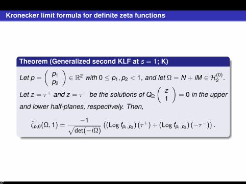
Kronecker limit formula for definite zeta functions

Theorem (Generalized second KLF at s = 1; K)

Let p =

(p1p2

)∈ R2 with 0 ≤ p1,p2 < 1, and let Ω = N + iM ∈ H(0)

2 .

Let z = τ+ and z = τ− be the solutions of QΩ

(z1

)= 0 in the upper

and lower half-planes, respectively. Then,

ζp,0(Ω,1) =−1√

det(−iΩ)

((Log fp1,p2 ) (τ+) + (Log fp1,p2 ) (−τ−)

).

37

Kronecker limit formula for indefinite zeta functions

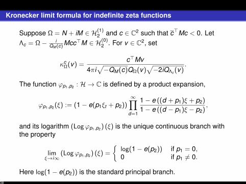
Suppose Ω = N + iM ∈ H(1)2 and c ∈ C2 such that c>Mc < 0. Let

Λc = Ω− iQM (c) Mcc>M ∈ H(0)

2 . For v ∈ C2, set

κcΩ(v) =

c>Mv4πi√−QM(c)QΩ(v)

√−2iQΛc (v)

.

The function ϕp1,p2 : H → C is defined by a product expansion,

ϕp1,p2 (ξ) := (1− e(p1ξt + p2))∞∏

d=1

1− e ((d + p1)ξ + p2)

1− e ((d − p1)ξ − p2),

and its logarithm (Logϕp1,p2 ) (ξ) is the unique continuous branch withthe property

limξ→i∞

(Logϕp1,p2 ) (ξ) =

log(1− e(p2)) if p1 = 0,0 if p1 6= 0.

Here log(1− e(p2)) is the standard principal branch.38

Kronecker limit formula for indefinite zeta functions

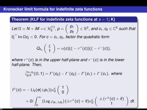
Theorem (KLF for indefinite zeta functions at s = 1; K)

Let Ω = N + iM =∈ H(1)2 , p =

(p1p2

)∈ R2, and c1, c2 ∈ C2 such that

cj> Im Ωcj < 0. For c = c1, c2, factor the quadratic form

QΛc

(ξ1

)= α(c)(ξ − τ+(c))(ξ − τ−(c)),

where τ+(c) is in the upper half-plane and τ−(c) is in the lowerhalf-plane. Then,

ζc1,c2p,0 (Ω,1) = I+(c2)− I−(c2)− I+(c1) + I−(c1), where

I±(c) = − Li2(e(±p1))κcΩ

(10

)+ 2i

∫ ∞0

(Logϕp1,±p2 ) (±τ±(c) + it)κcΩ

(± (τ±(c) + it)

1

)dt .

39

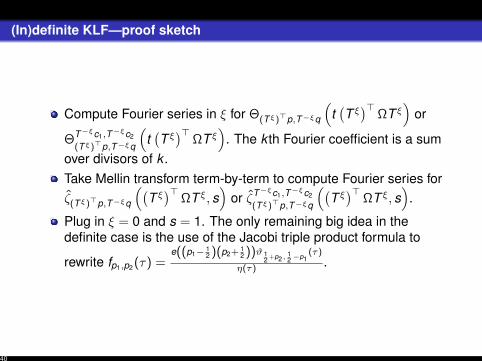
(In)definite KLF—proof sketch

Compute Fourier series in ξ for Θ(Tξ)>p,T−ξq

(t(T ξ)>

ΩT ξ)

or

ΘT−ξc1,T−ξc2

(Tξ)>p,T−ξq

(t(T ξ)>

ΩT ξ)

. The k th Fourier coefficient is a sumover divisors of k .Take Mellin transform term-by-term to compute Fourier series forζ(Tξ)>p,T−ξq

((T ξ)>

ΩT ξ, s)

or ζT−ξc1,T−ξc2

(Tξ)>p,T−ξq

((T ξ)>

ΩT ξ, s)

.

Plug in ξ = 0 and s = 1. The only remaining big idea in thedefinite case is the use of the Jacobi triple product formula to

rewrite fp1,p2 (τ) =e((p1− 1

2 )(p2+ 12 ))ϑ 1

2 +p2,12−p1

(τ)

η(τ) .

40

Indefinite KLF—proof sketch

In indefinite case, we obtain the following expression for the k thFourier coefficient of the theta function when k 6= 0.

bk (ξ) =∑n|k

|n|∫ ∞−∞

ρc1,c2M

((ξ1

)nt1/2

)

· e(

QΩ

(ξ1

)n2t + p>

(ξ1

)n)

e (−kξ) dξ.

Before taking the Mellin transform, we must shift some contoursof integration up and others down so that we get a convergentexpression afterwards.

bk (ξ) =∑n2|k

|n|∫ ∞+iλ( k

n ,n)

−∞+iλ( kn ,n)

ρc1,c2M

((ξ1

)nt1/2

)

· e(

QΩ

(ξ1

)n2t + p>

(ξ1

)n)

e (−kξ) dξ.

41

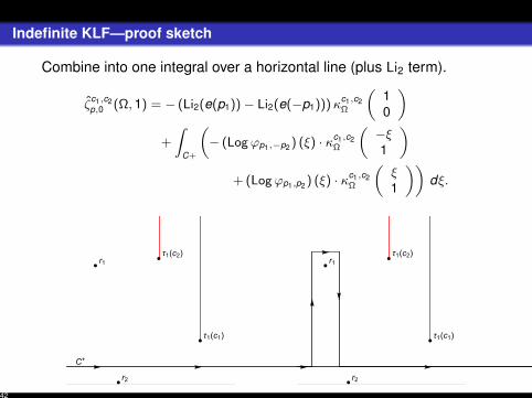
Indefinite KLF—proof sketch

Combine into one integral over a horizontal line (plus Li2 term).

ζc1,c2p,0 (Ω, 1) = − (Li2(e(p1)) − Li2(e(−p1)))κ

c1,c2Ω

(10

)+

∫C+

(− (Logϕp1,−p2 ) (ξ) · κc1,c2

Ω

(−ξ1

)+ (Logϕp1,p2 ) (ξ) · κc1,c2

Ω

(ξ1

))dξ.

r1

r2

τ1(c1)

τ1(c2)

C+

r1

r2

τ1(c1)

τ1(c2)

42

Indefinite KLF—proof sketch

After moving above the zeros of the QΛcj

(±ξ1

), the integral

can be split up into pieces for c1 and c2.Finally, we collapse the contours onto the branch cuts of

κcjΩ

(ξ1

).

r1

r2

τ1(c1)

τ1(c2)r1

r2

τ1(c1)

τ1(c2)

43

Example

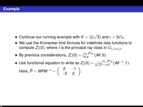
Continue our running example with K = Q(√

3) and c = 5OK .We use the Kronecker limit formula for indefinite zeta functions tocompute Z ′I (0), where I is the principal ray class in Clc,∞2.

By previous considerations, Z ′I (0) = ζc1,P3c10,q (iM,0).

Use functional equation to write as Z ′I (0) = −i2√

3ζc1,P3c1−q,0 (iM−1,1).

Here, P = MPM−1 =

(2 −1−3 2

).

44

Example

If we use the indefinite KLF directly, the branch cut of κP3c1Ω

(ξ1

)starts very close to the real axis, at ξ = −2340+i

√3

4053 . Convergence isslow in practical terms. Instead, split into three pieces:

ζc1,P3c1−q,0 (−Ω−1,1) = ζc,Pc

−q0,0(−Ω−1,1) + ζc,Pc−q1,0(−Ω−1,1) + ζc,Pc

−q2,0(−Ω−1,1),

where c =

(13

), q0 = 1

5

(10

), q1 = 1

5

(21

), and q2 = 1

5

(24

).

Now, branch cuts start at ±3+i√

36 , and convergence is rapid.

I0(Pc) − I0(c) ≈ −0.0592384392 + 3.6568783902i

I1(Pc) − I1(c) ≈ −1.3373302109 + 0.5247781254i

I2(Pc) − I2(c) ≈ 2.6405758737 + 0.5247781254i

Obtain Z ′I (0) ≈ 1.3586306534, just as before.

45

Thanks & Questions

Thank you for attending my talk! Thank you to Larry Rolen and theother organizers.

Questions?

46