Incremental Fusion of Structure-from-Motion and GPS

using Constrained Bundle Adjustments

Maxime Lhuillier

Institut Pascal, UMR 6602, CNRS/UBP/IFMA

24 avenue des Landais,

63177 Aubiere Cedex, France.

Mail: Maxime.Lhuillier [AT] free.fr

Tel: +33(0)4 73 40 75 93

Fax: +33(0)4 73 40 72 62

http://maxime.lhuillier.free.fr

The reference of this paper is: Maxime Lhuillier, Incremental Fusion ofStructure-from-Motion and GPS using Constrained Bundle Adjustments, IEEETransactions on Pattern Analysis and Machine Intelligence, 34(12), 2012.

The published version of this paper is available athttp://ieeexplore.ieee.org/xpl/tocresult.jsp?isnumber=6332439

Copyright c©2012 IEEE

1

Incremental Fusion of Structure-from-Motion and

GPS using Constrained Bundle Adjustments

Maxime Lhuillier

Abstract

Two problems occur when bundle adjustment (BA) is applied on longimage sequences: the large calculation time and the drift (or error accu-mulation). In recent work, the calculation time is reduced by local BAsapplied in an incremental scheme. The drift may be reduced by fusion ofGPS and Structure-from-Motion. An existing fusion method is BA min-imizing a weighted sum of image and GPS errors. This paper introducestwo constrained BAs for fusion, which enforce an upper bound for thereprojection error. These BAs are alternatives to the existing fusion BA,which does not guarantee a small reprojection error and requires a weightas input. Then the three fusion BAs are integrated in an incrementalStructure-from-Motion method based on local BA. Lastly, we will com-pare the fusion results on long monocular image sequences and low costGPS.

1 Introduction

Bundle adjustment (BA) is an iterative method of estimating camera poses and3d points detected in an image sequence [12]. The resulting poses and pointsminimize a sum of squared reprojection errors.

Recent BA developments mainly concern accelerations for long sequencessuch as multicore BA [13], conjugated gradient [1], and local BA (LBA) [10].

Another BA topic is fusion of data coming from several sensors. Fusionis useful for reducing the error accumulation of Structure-from-Motion (SfM),which is unavoidable for long image sequence (especially if the camera is monoc-ular). Global BA is used in aerial Photogrammetry to combine image, inertialand GPS measures: the cost function minimized by BA is a sum of image,inertial and GPS terms weighted by measure covariances [8]. There is alsoan attempt to include the GPS pseudo-ranges directly as measures in BA [3].In a different context, the reprojection errors of 3d points involved in BA aremodified such that points are constrained into vertical planes stored in a GISdatabase [7]. Recent work combines GPS and image measures [5] (or inertialand image measures [9]) using LBA, which minimizes a weighted sum of GPS(or inertial) and image terms. In [9], several weights are experimented. In [5],

2

the experiments are limited to a small sequence (70 m) and the GPS term isdefined by a high order polynomial.

In [6], new constrained BAs are introduced for SfM-GPS fusion. TheseBAs enforce an upper bound for the reprojection error, while the other fusionBAs [8, 9, 5] do not guarantee a small reprojection error and requires a weight.This paper also compares the results of the fusion BAs in a context which isuseful for applications: the incremental SfM based on LBA [10]. In experiments,low cost GPS and monocular (calibrated) camera are mounted on a car movingin urban area. The trajectory length is larger (4 km) than in the previous works.

The current paper is an improved version of [6]. The prerequisites detail ourassumptions (Section 2.1) and studies our upper bound-based fusion scheme ina simple case (Section 2.2): if the sum of squared reprojection errors is approx-imated by one quadratic Taylor expansion. Section 3 provides a brief overviewof BAs which solve the SfM-GPS fusion problem. Only sparse Levenberg-Marquardt [12] (second order) based methods are considered here. Section 4introduces our two constrained BAs for fusion, which involve inequality con-straint. Section 5 provides the detailed algorithms (useful for re-implementers).Lastly, Section 6 shows experiments in the same context as [6].

The additional contributions over [6] includes Section 2.2 and new exper-iments. Section 2.2 provides interesting properties and helps to convince thereader that SfM-GPS fusion is possible without calculation of SfM covariance.The properties detail the link between the ǫ-indifference region [2] defined byour upper bound, the SfM covariance (that we do not estimate), and the GPSlocations where fusion is possible.

The new experiments show the robustness of the fusion methods againstseveral important factors: upper bounds for image error and track lengths,time shift between GPS and video recorders, frequency of GPS perturbations,number of iterations, incomplete GPS data. Lastly, a 5 km long sequence isexperimented with GPS providing altitude (the GPS in [6] does not).

2 Prerequisites

Section 2.1 introduces notations and assumptions. Section 2.2 details our fusionscheme when the sum of squared reprojection errors is approximated by onequadratic Taylor expansion.

2.1 Main notations and assumptions

The Euclidean norm is ||.||. Different fonts are used for vectors (e.g. x), matrices(e.g. H) and function/real (e.g. e). Vector x concatenates the 3d parameters(camera poses and 3d points) and e(x) is the sum of squares of reprojectionerrors of x.

In this paper, we assume that the starting/input x of fusion BA is theminimizer x∗ of e, i.e. ∀x, e(x∗) ≤ e(x). Standard BA (not fusion BA) providesx∗.

3

Let x1 be location(s) of the camera. The variable ordering is such thatxT =

(

xT1 xT

2

)

. Let P =(

I 0)

be such that x1 = Px.Let x

gps1 be the location(s) of the camera provided by GPS at the same

time(s) as x1. Assuming that the GPS drift (or accumulation error) is boundedand that of SfM is not, the ideal output x of fusion BA meet x1 ≈ x

gps1 .

Vector x2 concatenates all 3d points, all rotations of the camera, and thecamera locations without GPS data.

Let et be a threshold which is slightly greater than the minimum e(x∗) of e.In our context, the final/output x of fusion BA is assumed to be acceptable ifits reprojection error is similar to the minimum of e, i.e.

e(x) < et. (1)

Last, we assume that H > 0, i.e. the hessian of e is positive definite in aneighborhood of x∗.

2.2 Quadratic Taylor approximation

Let q and H∗ be the quadratic Taylor expansion and Hessian of e at x∗. Sincee gradient is zero at x∗,

e(x∗ + ∆) ≈ q(∆) = e(x∗) + 0.5∆TH∗∆. (2)

In the paper we use block-wise notations(

x∗

1 x1 ∆1

x∗

2 x2 ∆2

)

=(

x∗ x ∆)

,

(

H1 HT21

H21 H2

)

= H∗. (3)

Assume that ∆1 is a step of x∗

1 to remove (or to reduce) the SfM drift, i.e.x∗

1 +∆1 = xgps1 . Now we should find x such that both Eq. 1 and x1 = x∗

1 +∆1

are meet.The set of values x defined by Eq. 1 is called ǫ-indifference region ([2], p.171)

where ǫ = et − e(x∗). Since ǫ is small and H∗ > 0, Eq. 2 is used to approximatethe ǫ-indifference region by ellipsoıd ([2], p.172)

Eǫx∗ = {x∗ + ∆, q(∆) ≤ e(x∗) + ǫ}. (4)

Now we should find x ∈ Eǫx∗ such that x1 = x∗

1 + ∆1. In other words, xgps1

should be in the ellipsoıd projection

Eǫx∗

1

= {x1, ∃x2,(

xT1 xT

2

)T∈ Eǫ

x∗}

= {x∗

1 + ∆1, ∃∆2, q(

(

∆1

∆2

)

) ≤ e(x∗) + ǫ}. (5)

Lemma 1 is useful to explicit Eǫx∗

1

.

Lemma 1: Function ∆2 7→ q((

∆T1 ∆T

2

)T) has minimum

q(

(

∆1

−H−12 H21∆1

)

) = e(x∗) + 0.5∆T1 C

−11 ∆1, (6)

4

where C1 = (H1 − HT21H

−12 H21)

−1 is the top-left block of H∗−1.

Proof: Thanks to H∗ > 0 and Section 6.1 of [12], H1 − HT21H

−12 H21 is the Schur

complement of H2 in H∗ and C1 is the top-left block of H∗−1. Furthermore, H∗ > 0

implies H2 > 0. Thus, quadratic function ∆2 7→ q((

∆T1 ∆T

2

)T) has minimizer

−H−12 H21∆1 and minimum

e(x∗) + 0.5∆T1

(

I

−H−12 H21

)T

H∗(

I

−H−12 H21

)

∆1. (7)

�

Thanks to Lemma 1, we can use ∆2 = −H−12 H21∆1 in Eq. 5 and obtain

Eǫx∗

1

= {x∗

1 + ∆1,∆T1 C

−11 ∆1 ≤ 2ǫ}. (8)

Theorem 1 summarizes the derivations of Section 2.2.

Theorem 1: Thanks to the quadratic Taylor approximation of e at x∗, thefusion problem defined by

e(x) ≤ et and x1 = xgps1 (9)

has solution(s) x if and only if xgps1 is in the ellipsoıd Eǫ

x∗

1

(Eq. 8) where ǫ =

et − e(x∗) and C1 = (H1 − HT21H

−12 H21)

−1. In this case, e(x) is minimized bychoosing

x2 = x∗

2 − H−12 H21(x

gps1 − x∗

1). (10)

If xgps1 /∈ Eǫ

x∗

1

, Theorem 1 can still be used to fuse SfM and GPS incompletely:

we replace xgps1 by x

gps1 ∈ Eǫ

x∗

1

such that xgps1 is close as possible to x

gps1 .

Lastly, we provide a probabilistic interpretation of C1 and Eǫx∗

1

. Remind that

x∗ is the minimizer of sum of squared reprojection errors. Under the assumptionthat the image noise follows the zero-mean normalized Gaussian vector, the x∗

covariance is approximated by H∗−1 [4]. Then we see that C1 is the covariancematrix of x∗

1 and Eǫx∗

1

is an uncertainty ellipsoıd of x∗

1.

3 BA candidates for SfM-GPS fusion

Here we review three BAs which fuse SfM and GPS. They meet the requirementsof Section 2.1.

5

3.1 UBA: BA without explicit constraint

Such a BA was used to combine measurements from different sensors [8]. Werefer to it as UBA or “unconstrained BA”. A sum of weighted terms is mini-mized:

eU (x) = e(x) + β||Px − xgps1 ||2. (11)

Here the problems are the adequate choice of weight β and the risk of inlier lossdue to the term β||Px − x

gps1 ||2. The inliers are the detected points involved

in e such that the reprojection error is less than a threshold. These problemsare similar if we generalize β||.||2 by a quadratic form defined by a covariancematrix. In our framework, the UBA output is ignored if e(x) > et

3.2 IBA: BA with inequality constraint

Another method uses penalty function ([2], p.141). In our context, the iterationsof this constrained BA enforce the inequality constraint in Eq. 1, i.e. cI(x) > 0where cI(x) = et − e(x). Here we minimize

eI(x) = γ/cI(x) + ||Px − xgps1 ||2 (12)

where γ > 0. Function x 7→ ||Px−xgps1 || is minimized while the penalty function

γ/cI(x) enforces the inequality constraint. Penalty is the main (positive infinite)term in the neighborhood of cI(x) = 0, and it does not change the minimizerstoo much of x 7→ ||Px− x

gps1 ||2 elsewhere.

Although the principle is simple, such an IBA was not used before for fusionof SfM and another sensor.

3.3 EBA: BA derived from equality constraints

BAs in [12] minimize e(x) subject to equality constraint c(x) = 0. At firstglance, we could try c(x) = Px− x

gps1 since we would like x1 ≈ x

gps1 .

One iteration improves x by adding step ∆ subject to the linearized con-straint c(x + ∆) ≈ c(x) + ∂c

∂x∆ = 0. Like unconstrained BA, damping is used

to define ∆ between the Gauss-Newton step, which minimizes the quadraticTaylor expansion of e, and a gradient descent step. The Taylor expansionsrequire a small enough ∆, which in turn requires a small enough value of||c(x)|| = || ∂c

∂x∆||.

Now we see that c(x) = Px − xgps1 can not be used: on the one hand the

constrained BAs in [12] require small ||c(x)||, while on the other c(x∗) = x∗

1 −x

gps1 may have large modulus since it is the drift between SfM and GPS.

Therefore we introduce EBA, which is derived from a constrained BA in [12].EBA is a different method and c is replaced by another function

cα(x) = Px− ((1 − α)xgps1 + αx∗

1) where α ∈ [0, 1]. (13)

6

Note that Eq. 13 is the same as Eq. 14 in [6], i.e. cα(x) = c(x)−αc(x∗). Eq. 13makes easier the understanding of cα(x) = 0: x1 is a linear interpolation of x

gps1

and x∗

1.Eq. 13 implies c1(x

∗) = 0 and c0(x) = c(x). EBA decreases α progressivelyfrom 1 (no constraint before all iterations) to 0 (full constraint). The final valueof α may be different to 0 and this measures the success of fusion between GPSand image data from α = 1 (failure) to α = 0 (100% success). A decreaseof α may produce an increase of e(x), but this increase is moderated since weintegrate in EBA the reduction method (a constrained BA in Section 4.4 of [12]).This is useful to meet Eq. 1.

Note that EBA minimizes α and the (integrated) reduction method mini-mizes e(x). For the paper clarity, the reduction method and EBA are describedin two different Sections 4.3 and 4.4.

4 Iteration of BAs

Section 4 describes the iterations of Levenberg-Marquardt (LM), IBA and EBA(the former is useful to explain the latters). The supplementary material showsthat successful iteration is possible in all cases.

The quadratic Taylor expansion of e at x is

e(x + ∆) ≈ e(x) + gT ∆ + 0.5∆TH∆ (14)

where g and H are the gradient and hessian of e. The projection functionE : R

n → Rm meets e(x) = ||E(x)||2. Let J be the jacobian of E at x. We have

g = 2JT E(x) and use the Gauss-Newton approximation H ≈ 2JTJ. We assumeJTJ > 0 since H > 0 (Section 2.1).

4.1 Levenberg-Marquardt without constraint

The LM iteration to minimize e(x) without constraint is the following [11] (UBAminimizes a different function using LM). Efficient sparse methods are used tosolve (H+λdiag(H))∆ = −g for the current value of x and a damping coefficientλ > 0. If e(x + ∆) < e(x), the iteration is successful: x is replaced by x + ∆

and λ is replaced by λ/10. Otherwise, λ is replaced by 10λ.

4.2 IBA

The method is the same as in Section 4.1, except for the calculation of ∆. Letxi be a coefficient of x and f(x) = γ/(et − e(x)). We have

∂f

∂xi

=γ

(et − e)2∂e

∂xi

∂2f

∂xi∂xj

=γ

(et − e)3((et − e)

∂2e

∂xi∂xj

+ 2∂e

∂xi

∂e

∂xj

). (15)

7

Then, we use the Gauss-Newton approximation H ≈ 2JTJ and obtain the gra-dient and hessian of eI :

gI =γ

(et − e)2g + 2PT (Px− x

gps1 )

HI ≈2γ

(et − e)3((et − e)JTJ + ggT ) + 2PTP. (16)

Now, the linear system (HI + λdiag(HI))∆ = −gI is solved. This can not besolved as in Section 4.1 since HI is not sparse due to the dense term ggT .Section 5.1 provides an efficient method to solve this linear system.

4.3 Reduction Method (BA with equality constraint)

Now the LM iteration to minimize e(x) subject to constraint c(x) = 0 is de-scribed [12]. We use notations

(

x1 ∆1 g1

x2 ∆2 g2

)

=(

x ∆ g)

,

(

H1 HT21

H21 H2

)

= H (17)

and jacobian(

C1 C2

)

of c at x. In our case, C1 = I, C2 = 0 and step ∆ is suchthat

c(x + ∆) ≈ c(x) + C1∆1 + C2∆2 = c(x) + ∆1 = 0. (18)

Then, ∆ is

∆(∆2) =(

−c(x)T ∆T2

)T. (19)

Thanks to Eq. 14 and ∆ = ∆(∆2), we obtain

e(x + ∆(∆2)) ≈ e2 + ∆T2 g2 + 0.5∆T

2 H2∆2 (20)

where

e2 = e(x) − gT1 c(x) + 0.5c(x)TH1c(x)

g2 = g2 − H21c(x) (21)

Step ∆2 meets (H2 +λdiag(H2))∆2 = −g2. Now the iteration is the same asin Section 4.1 using ∆ = ∆(∆2).

4.4 From Reduction Method to EBA

Assume that EBA is the reduction method using the constraint in Eq. 13.A problem is the descending condition e(x + ∆(∆2)) < e(x) to test step∆ = ∆(∆2). In our fusion context, the initial value of x is x∗, which mini-mizes e. So the descending condition can not be meet at the very beginning ofEBA. However, we remind that our condition for fusion is Eq. 1. We solve thisproblem, substituting the descending condition by

e(x + ∆(∆2)) < et. (22)

8

Now the ∆2 calculation in a successful EBA iteration is concisely writtenas: find positive δ and λ such that

g2 = g2 − H21cα−δ(x)(H2 + λdiag(H2))∆2 = −g2

e(x +(

−cα−δ(x)T ∆T2

)T) < et.

(23)

Then we add ∆ =(

−cα−δ(x)T ∆T2

)Tto x, and subtract δ from α. The

detailed algorithm is in Section 5.2. According to the supplementary material,Eqs. 23 have a solution thanks to small enough δ and large enough λ.

5 Implementation

Now we will explain how to implement efficiently IBA (Section 5.1) and EBA(Section 5.2).

5.1 IBA

In Section 4.2, (HI + λdiag(HI))∆ = −gI should be solved efficiently. Let ~H andg be such that

HI + λdiag(HI) = ~H + ggT , g =

√

2γ

(et − e)3g. (24)

Basic computation shows that

(~H + ggT )−1 = (I−~H−1ggT

1 + gT ~H−1g)~H−1. (25)

We introduce a = −~H−1gI , b = ~H−1g, and obtain

∆ = −(~H + ggT )−1gI = a −gTa

1 + gT bb. (26)

Now we explain how to estimate a and b. According to Eqs. 16 and 24, ~H

has the sparse structure of JTJ. More precisely [4], we have ~H =

(

U W

WT V

)

and

~H > 0 where U is a 6 × 6 block-wise matrix, V is a 3 × 3 block-wise invertiblediagonal matrix, and W is a 6 × 3 block-wise matrix such that the (i, j) blockis zero if the j-th 3d point is not seen in the i-th image. So linear systems~Ha = −gI and ~Hb = g are solved using the same efficient sparse method [4] asthe linear system (H + λdiag(H))∆ = −g.

The algorithm in C style is the following. The inputs are reprojection errore(x) = ||E(x)||2, GPS location(s) x

gps1 , initial x which minimizes e (i.e. x = x∗),

maximum number of iterations Itmax, and threshold et. The output is x suchthat e(x) < et and eI(x) has the smallest possible value.

9

err = γ/(et − e(x)) + ||Px− xgps1 ||2;

UpdateD = 1; λ = 0.001;for (It = 0; It < Itmax; It++) {

// derivative update and estimation of ∆

if (UpdateD) {UpdateD = 0;g = 2JT E(x); H = 2JTJ; // J is the jacobian of E at x

gI = γ(et−e)2 g + 2PT (Px − x

gps1 ); H = γ

(et−e)2 H + 2PTP;

g =√

2γ(et−e)3 g; // now, HI = H + ggT (don’t store HI)

}~H = H + λdiag(H + ggT );solve ~H

(

a b)

=(

−gI g)

∆ = a − (gT a)/(1 + gTb)b;// try to decrease eI

if (e(x + ∆) ≥ et) { λ = 10λ; continue; }err′ = γ/(et − e(x + ∆)) + ||P(x + ∆) − x

gps1 ||2;

if (err′ < err) {x = x + ∆;if (0.9999err < err′) break; // convergence is too slowerr = err′; UpdateD = 1; λ = λ/10;

} else λ = 10λ;}

5.2 EBA

Solving the linear system of Eqs. 23 is the main calculation. At first glance, thisshould be done for each tried (λ, δ) since g2 depends on cα−δ(x). Fortunately,we can reduce the number of these calculations. We solve ∆a

2 and ∆b2 such that

(H2 + λdiag(H2))(

∆a2 ∆b

2

)

=(

−g2 H21

)

(27)

and obtain ∆2 = ∆a2 + ∆b

2cα−δ(x). Now we see the improvement: once thelinear system in Eq. 27 is solved, ∆2 is obtained very efficiently for all tried δ.

We try δ ∈ {α, α/2, · · ·α/210} in the decreasing order. If all δ above fail, wechange the EBA iteration using ∆T =

(

0T (∆a2)

T)

. Then we find λ such thate(x + ∆) < e(x) as in unconstrained BA (U-iteration).

Remind that EBA minimizes α, but it is interesting to obtain the smalleste(x) for a given α. Thus, we alternate successful iteration with δ > 0 (E-iteration) and successful U-iteration to decrease e as much as possible. TheU-iterations do not update α. If α = 0, only U-iterations are applied untilconvergence.

The following algorithm in C style provides the remaining details. The inputsare reprojection error e(x) = ||E(x)||2, constraint c, initial x which minimizese, maximum number of iterations Itmax, and threshold et. The output is (x, α)such that e(x) < et, x1 = (1 − α)xgps

1 + αx∗

1 and the smallest α as possible.

10

err = e(x); c∗ = c(x);UpdateD = 1; λ = 0.001; α = 1;αold = 1; // αold is used to alternate E- and U-iterationsfor (It = 0; It < Itmax; It++) {

// derivative update and estimation of ∆a2 and ∆b

2

if (UpdateD) {UpdateD = 0;g = JT E(x); H = JTJ; // J is the jacobian of E at x(

g1

g2

)

= g;

(

H1 HT21

H21 H2

)

= H;

}solve (H2 + λdiag(H2))

(

∆a2 ∆b

2

)

=(

−g2 H21

)

// E-iteration: try to decrease α with bounded eif (0 < α && αold == α) {

for (It2 = 0, α′ = 0; It2 < 10; It2++) {cα′(x) = c(x) − α′c∗;∆2 = ∆a

2 + ∆b2cα′(x);

∆T =(

−cα′(x)T ∆T2

)

; err′ = e(x + ∆);if (err′ < et) break; // success if trueα′ = 1

2 (α + α′);}if (It2 < 10) { // success if true

αold = α; α = α′;x = x + ∆;err = err′; UpdateD = 1; continue;

}}// U-iteration: try to decrease e without α update∆2 = ∆a

2 ; ∆T =(

0T ∆T2

)

; err′ = e(x + ∆);if (err′ < err) {

x = x + ∆;if (α == 0 && 0.9999err < err′) break;αold = α, err = err′; UpdateD = 1; λ = λ/10;

} else λ = 10λ;}

6 Experiments

6.1 Integrating fusion to LBA-based SfM

SfM [10] reconstructs the very beginning of the sequence using standard methodsand then alternates the following steps: (1) a new keyframe is selected fromthe input video and interest points are matched with the previous keyframeusing correlation (2) the new pose is estimated using Grunert’s method andRANSAC (3) new 3d points are reconstructed from the new matches and (4)LBA refines the geometry of the n-most recent keyframes. In the LBA context, xconcatenates the 6D poses of the n-most recent images and the 3d points which

11

have observation(s) in these images, e(x) is the sum of squared reprojectionerrors of these 3d points in the N most recent images. There is no gaugefreedom and H > 0. Step 4 uses n = 3 and N − n = 7 [10].

Our paper adds step (5), a fusion step which is the local version of UBA, IBAor EBA: e is the reprojection error of the LBA which refines the geometry of thek-most recent keyframes. The minimizer x∗ of e is estimated before each fusionLBA using a single iteration of standard LBA. Vector x1 is the 3d location ofthe most recent key-frame. Fusion LBA does not involve point outliers sincethey are rejected by steps (3-4) as in [10].

UBA, IBA and EBA run under the same conditions: same keyframes, samematches, same maximum number of iterations (Itmax = 4), same k and et. Ourdefault values are k = 40 and et = 1.052e(x∗), i.e. a RMS increase of 5% isaccepted for fusion. The other (default) parameters of UBA and IBA are

β =e(x∗)

||Px∗ − xgps1 ||2

, γ =et − e(x∗)

10||Px∗ − x

gps1 ||2. (28)

These weights are such that the ratio between image term and GPS term in eU

(eI , respectively) is 1 (0.1, respectively) before the fusion optimization.Step (5) is used in the main loop once the SfM result is registered in the

GPS coordinate system. The registration method is the following. First weselect times t0 = 0 and t1 such that the distance between the two GPS positionsis greater than 10 meters. Then we define the vertical direction in the SfM resultassuming that both x-axis and motion of the camera are horizontal between t0and t1. Now three points are defined in both coordinate systems (SfM andGPS) and a similarity transformation is estimated from these points. Finally,the SfM result is mapped in the GPS coordinate system using the similaritytransformation.

6.2 Notations

The 3d location of keyframes are provided by six methods: SfM, GPS, GT(ground truth), UBA, IBA and EBA.

Let a and b be two different methods that we would like to compare. Let liaand ei

a be the 3d location and the reprojection error (RMS) provided by methoda at the i-th keyframe. We study the distribution of ∀i, ||lia − lib||, where a ∈{SfM, GPS, UBA, IBA, EBA}, b ∈ {GPS, GT}. Its mean, standard deviationand maximum are mb

a, σba and ∞b

a in meters. We also study the distribution of∀i, ei

a/ei

SfM, where a ∈ {UBA, IBA, EBA}. Its mean, standard deviation and

maximum are m2da , σ2d

a and ∞2da . We refer to these distributions as location

errors and image errors, respectively. Here lia and eia are estimated after the

calculation of the entire sequence by method a.

6.3 Experimental conditions for sequence 1

Our GPS and camera are mounted on a car. Its trajectory has straight lines,sharp curves, traffic circles, stop and go due to traffic lights. It is 4 km long.

12

Figure 1: Images of sequence 1.

f mgpsf σgps

f ∞gpsf mgt

f σgtf ∞gt

f m2df σ2d

f

SfM 165 172 591 164 172 592 1 0UBA 2.61 2.40 11.3 5.59 3.18 14.0 1.04 .044IBA 1.24 1.50 8.47 4.57 2.83 12.1 1.05 .046EBA 2.48 2.27 10.5 5.49 3.12 14.0 1.04 .045GPS 0 0 0 4.28 2.34 12.2 - -

Table 1: Location errors and image errors using the default parameters. If f ∈{UBA, IBA, EBA}, ∞2d

f ∈ [1.28, 1.3].

The scene includes low and high buildings, trees and moving vehicles.The GPS is low cost (Ublox Antaris 4). It provides one 2D location (longi-

tude, latitude) at 1Hz and the altitude is set to 0. Once the GPS coordinatesare converted to euclidean coordinates in meters, linear interpolation is usedto obtain a 3d GPS location at all times. The ground truth is provided at10Hz by IXSEA LandINS and RTK (not low cost) GPS. We have mgt

gps = 4.28,σgt

gps = 2.34 and ∞gtgps = 12.2, so the name “low cost GPS” is confirmed.

The camera is monocular and calibrated; it points forward and provides 640×352 images (Fig. 1) at 25 Hz. 2480 keyframes are selected from 14850 images,such that there are about 400 Harris point matches between three consecutivekeyframes. We assume that the distance between camera and GPS antennais small in comparison to GPS accuracy: the GPS coordinates of the camera(xgps

1 ) are approximated by those of the GPS antenna.

6.4 Comparison of UBA, IBA and EBA

Here we compare the methods using the default parameters in Section 6.1.Tab. 1 shows the location errors. The three fusions (UBA, IBA, EBA) greatlyreduce the errors relative to GPS to about 2 meters. The errors relative toground truth are also greatly reduced to about 5 meters, which is the magnitudeorder of the GPS accuracy. However, the fusion methods are not able to improvethe mean of GPS accuracy since the fusion errors are slightly larger than thepure GPS errors. According to values of mGPS

a and mGTa , the best results are

obtained by IBA, followed by EBA and UBA. Tab. 1 also shows the imageerrors. We check that they are acceptable for all fusion BAs since they show

13

Figure 2: Top views of trajectories: GPS+SfM (top left), GPS+IBA (bottom left).Local view (right) of GPS (black crosses), GT (black dots), UBA (red dots), IBA(green dots), EBA (blue dots). One dot is one keyframe.

that the increase of RMS reprojection errors per keyframe due to fusion is about5%. RMS ei

SfM ranges from 0.37 to 0.54 pixel (the mean is 0.44), which implies

that eif ≤ 0.702 pixel ∀f, ∀i.

Fig. 2 shows top views of GPS, SfM and IBA trajectories. We see the drift ofSfM compared to GPS (top left). At this scale, it is difficult to see a differencebetween GPS and IBA (bottom left). The same observation can be done forUBA and EBA. Fig. 2 also shows a local view of the 3d locations provided bythe fusion BAs (right), in the case where there are high buildings at the roadborder. The car moves from right to left. We see that the trajectory shapes ofthe fusion BAs are better than that of the GPS: fusion trajectories are smoothlike GT trajectory, GPS trajectory (using linear interpolation) is not smooth ata point on the left. We can also see that the GPS does not provide a good localscale factor to the trajectory.

The mean times of U-/I-/EBA are 0.25, 0.27 and 0.28 seconds for eachkeyframe, respectively. Here we use a core 2 duo 2.5Ghz laptop, sparse imple-mentation of hessians, and Cholesky factorization of reduced camera system tosolve the LM linear systems [12].

6.5 Weight changes for UBA and IBA

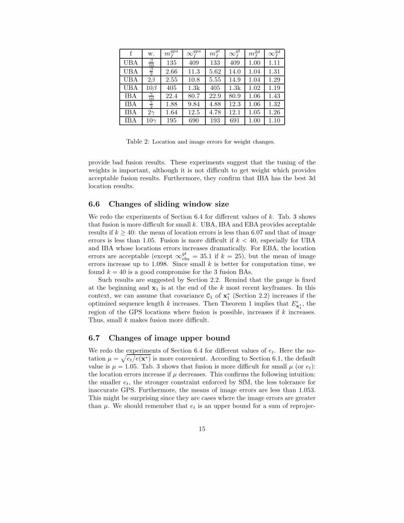
Remember that UBA and IBA require choosing weights β and γ, respectively.So we re-do the UBA and IBA fusions of Section 6.4 using different weightsaround the default values in Eq. 28. The results are given in Tab. 2. We cansee that the fusion results are similar if we divide or multiply the weights by 2.We can also see that large changes of weight (division or multiplication by 10)

14

f w. mgpsf ∞gps

f mgtf ∞gt

f m2df ∞2d

f

UBA β10 135 409 133 409 1.00 1.11

UBA β2 2.66 11.3 5.62 14.0 1.04 1.31

UBA 2β 2.55 10.8 5.55 14.9 1.04 1.29UBA 10β 405 1.3k 405 1.3k 1.02 1.19IBA γ

10 22.4 80.7 22.9 80.9 1.06 1.43IBA γ

2 1.88 9.84 4.88 12.3 1.06 1.32IBA 2γ 1.64 12.5 4.78 12.1 1.05 1.26IBA 10γ 195 690 193 691 1.00 1.10

Table 2: Location and image errors for weight changes.

provide bad fusion results. These experiments suggest that the tuning of theweights is important, although it is not difficult to get weight which providesacceptable fusion results. Furthermore, they confirm that IBA has the best 3dlocation results.

6.6 Changes of sliding window size

We redo the experiments of Section 6.4 for different values of k. Tab. 3 showsthat fusion is more difficult for small k. UBA, IBA and EBA provides acceptableresults if k ≥ 40: the mean of location errors is less than 6.07 and that of imageerrors is less than 1.05. Fusion is more difficult if k < 40, especially for UBAand IBA whose locations errors increases dramatically. For EBA, the locationerrors are acceptable (except ∞gt

eba = 35.1 if k = 25), but the mean of imageerrors increase up to 1.098. Since small k is better for computation time, wefound k = 40 is a good compromise for the 3 fusion BAs.

Such results are suggested by Section 2.2. Remind that the gauge is fixedat the beginning and x1 is at the end of the k most recent keyframes. In thiscontext, we can assume that covariance C1 of x∗

1 (Section 2.2) increases if theoptimized sequence length k increases. Then Theorem 1 implies that Eǫ

x∗

1

, the

region of the GPS locations where fusion is possible, increases if k increases.Thus, small k makes fusion more difficult.

6.7 Changes of image upper bound

We redo the experiments of Section 6.4 for different values of et. Here the no-tation µ =

√

et/e(x∗) is more convenient. According to Section 6.1, the defaultvalue is µ = 1.05. Tab. 3 shows that fusion is more difficult for small µ (or et):the location errors increase if µ decreases. This confirms the following intuition:the smaller et, the stronger constraint enforced by SfM, the less tolerance forinaccurate GPS. Furthermore, the means of image errors are less than 1.053.This might be surprising since they are cases where the image errors are greaterthan µ. We should remember that et is an upper bound for a sum of reprojec-

15

mgtuba mgt

iba mgteba m2d

uba m2diba m2d

eba ∞2d∗

default 5.59 4.57 5.49 1.037 1.049 1.038 1.301

k=25 54.0 195 6.62 1.013 1.009 1.098 1.439k=30 65.2 43.3 4.99 1.018 1.021 1.070 1.501k=35 34.6 33.5 5.15 1.035 1.032 1.051 1.392k=45 5.84 4.56 5.74 1.029 1.042 1.032 1.291k=50 6.07 4.59 5.86 1.027 1.035 1.028 1.263

µ=1.01 112 76.3 6.16 1.003 1.004 1.052 1.288µ=1.03 94.9 5.01 5.40 1.022 1.049 1.039 1.314µ=1.07 5.58 4.55 5.51 1.037 1.053 1.038 1.299

δt=-2 89.9 229 396 1.025 1.021 1.054 1.394δt=-1 8.68 5.49 5.84 1.063 1.081 1.074 1.501δt=-.5 5.39 4.87 5.59 1.058 1.061 1.052 1.456δt=.5 5.91 4.71 5.79 1.032 1.048 1.035 1.283δt=1 6.40 5.39 6.50 1.030 1.054 1.039 1.337δt=2 10.3 7.64 7.99 1.060 1.071 1.073 1.444δt=3 20.9 16.1 9.56 1.048 1.056 1.100 1.569

L∞=6 5.39 4.57 5.28 1.041 1.059 1.043 1.320L∞=7 5.37 4.67 5.10 1.045 1.067 1.047 1.343L∞=8 11.9 9.47 4.99 1.035 1.045 1.048 1.360L∞=9 54.4 48.5 5.09 1.015 1.020 1.055 1.368L∞=∞ 54.5 54.4 4.45 1.005 1.007 1.036 1.277

Itmx=1 85.1 120 4.61 1.015 1.027 1.057 1.312Itmx=2 4.81 4.61 4.61 1.041 1.059 1.050 1.366Itmx=3 5.49 4.56 4.83 1.038 1.051 1.042 1.306

Table 3: Location and image errors for parameter changes.

16

p msfmuba msfm

iba msfmeba mgps

uba mgpsiba mgps

eba ∞2d∗

10 4.56 4.04 1.31 10.7 11.0 9.95 1.48100 4.56 4.04 1.31 11.9 14.5 10.1 1.64200 442 11.4 10.2 443 10.4 9.31 1.48400 10.7 12.3 10.1 6.43 7.93 4.67 1.48800 10.3 12.4 9.94 3.91 6.62 2.17 1.481600 9.91 10.4 9.88 1.57 1.46 0.76 1.48

Table 4: Location and image errors if i 7→ ligps − l

isfm has period p.

tion errors over the k most recent keyframes; it does not enforce upper boundfor individual keyframe. Last, we see that EBA is the most robust to small et.

6.8 Time shift between GPS and video recorders

We redo the experiments of Section 6.4 for different values of δt, which is the timeshift between GPS and video recorders (in seconds). The previous experienceshave δt = 0 and now we try δt 6= 0 as if the experimenter synchronizes the tworecorders manually. Tab. 3 shows that the results are not dramatically corruptedby a bad synchronization: δt ∈ {−.5, 0, .5, 1} provides acceptable results, δt > 2does not. Such a conclusion depends on the camera speed: the larger speed, themore corrupted GPS location for camera (xgps

1 ) due to δt 6= 0, the more difficultfusion. Here the speed is less than 60 km/h.

6.9 Upper bound for track lengths

Tab. 3 shows that the result of SfM-GPS fusion depends on L∞, the upperbound of the track lengths of image points. The default value is L∞ = 5, e.g.if a point is tracked over 13 consecutive frames, then we split this track into 2tracks with length 5 and 1 track with length 3. Large L∞ makes fusion moredifficult (except EBA).

6.10 Number of iterations

Tab. 3 shows the fusion results for values of Itmax. UBA and IBA fail ifItmax = 1. If Itmax ∈ {2, 3, 4}, we see that (1) the location and image errorsare acceptable (2) the greater Itmax, the smaller image error. Furthermore, thegreater Itmax, the smaller α returned by EBA. If Itmax = 4, the mean value isα = 0.0017. If Itmax = 1, α = 0.13. Remind that α > 0 means that the EBAfusion is incomplete (Section 3.3). Other examples of incomplete EBA fusionare α(µ = 1.01) = 0.76 and α(k = 25) = 0.56.

17

p mgpsuba mgps

iba mgpseba m2d

uba m2diba m2d

eba

20 36.8 31.9 1.80 1.04 1.04 1.0630 98.4 33.3 1.96 1.03 1.04 1.0740 32.3 7.84 9.87 1.03 1.04 1.1250 153 421 175 1.02 1.03 1.08

Table 5: Location and image errors for incomplete GPS data.

6.11 GPS as a periodic perturbation of SfM

We redo the experiments of Section 6.4 with GPS data such that ligps = lisfm +

10(

cos(2πi/p) sin(2πi/p) 0)T

, where p is the period of a circular perturba-

tion around the SfM result and(

0 0 1)T

is the vertical direction. Tab. 4shows the fusion results for several p. For small periods (p ≤ 100), the fusion

is mainly SfM since msfmf < mgps

f . For large periods (p ≥ 800), the fusion is

mainly GPS since msfmf > mgps

f . This suggests that the fusion only uses the

low frequencies of i 7→ ligps − lisfm.

6.12 Incomplete GPS data

The experiments of Section 6.4 are redone with incomplete GPS data, as ifGPS satellites are occluded due to high buildings. ligps is available and fusionis done if and only if (i modulo p) ∈ [0, p/2], where p is a period. Tab. 5 showsthe fusion results for several p. EBA has the best results, but fusion is moredifficult for large values of p.

6.13 Experiment for sequence 2

Sequence 2 has the following differences with sequence 1: 3d locations providedby Flytec GPS at 1 Hz, H.264 compressed video at 30 Hz by Gopro camera,19515 images reduced to 640 × 480, 4000 keyframes, 5 km long trajectory loop(max speed 77 km/h), the altitude variation is 51 m. The ground truth isunknown. The camera and GPS recorders are manually synchronized.

Fig. 3 shows the recorders, three images of the sequence, and a top view of theGPS and IBA trajectories obtained using the default parameters (Section 6.1).Tab. 6 provides the location and image errors. Now EBA has the best mean oflocation errors and the image errors are larger than those of sequence 1. RMSei

SfM ranges from 0.35 to 0.51 pixel (the mean is 0.45), which implies that

fusions always have eif ≤ 0.77 pixel.

7 Conclusion

Two constrained bundle adjustments IBA and EBA were introduced to fuseGPS and Structure-from-Motion data. They enforce an upper bound for the

18

Figure 3: Video (Gopro) and GPS (Flytec) recorders, 3 images of sequence 2, topview of the GPS and IBA trajectories.

f mgpsf σgps

f ∞gpsf m2d

f σ2df ∞2d

f

SfM 387 224 767 1 0 1UBA 3.62 3.09 15.1 1.06 0.06 1.43IBA 2.32 2.84 14.6 1.09 0.05 1.51EBA 2.12 1.58 10.4 1.13 0.09 1.48

Table 6: Location errors and image errors for sequence 2.

reprojection errors and are described in details. The experiments compare ourtwo BAs with the existing UBA (which minimizes a weighted sum of imageand GPS errors) in the difficult context of incremental Structure-from-Motionapplied on long urban image sequences and low cost GPS. We also study thefusion results for several parameter settings. Such experiments were not donebefore.

The three fusion BAs greatly improve the poses of the Structure-from-Motion; the resulting increases of reprojection errors are small. According toground truth, the resulting pose accuracies are similar to that of the GPS. TheGPS accuracy is slightly better (it is the only sensor which provides absolutedata, our monocular camera can not). EBA has two advantages: it does not re-quire weight choice and it is the most robust method to bad parameter settingsand bad experimental conditions. IBA may provide the best results for goodparameter settings. UBA is ranked #3.

Future work includes experiments with other fusion BAs, improvement toinitialize the visual reconstruction in the GPS coordinate system, parametersetting from knowledge of the GPS performance, fusion with other sensors,application to georeferenced 3d modeling.

19

References

[1] S. Agarwal, N. Snavely, S.M. Seitz and R. Szeliski, “Bundle Adjustment inthe Large”, Proc. ECCV’10.

[2] Y. Bard, Non-Linear Parameter Estimation, Academic Press Inc. (London)LTD, 1974.

[3] C. Ellum, “Integration of raw gps measurements into a bundle adjustment”,Proc. IAPRS series vol. XXXV, 2006.

[4] R. Hartley and A. Zisserman, Multiple View Geometry in Computer Vision,Cambridge University Press, 2000.

[5] H. Kume, T. Takemoti, T. Sato, and N. Yokoya, “Extrinsic camera param-eter estimation using video images and gps considering gps position accu-racy”, Proc. ICPR’10.

[6] M. Lhuillier, “Fusion of GPS and Structure-from-Motion using constrainedBundle Adjustments”, Proc. CVPR’11.

[7] P. Lothe, S. Bourgeois, F. Dekeyser, E. Royer, and M. Dhome, “Towardsgeographical referencing of monocular slam reconstruction using 3d citymodels: Application to real-time accurate vision-based localization”, Proc.CVPR’09.

[8] J. McGlone, The Manual of Photogrammetry, Fifth ed (ISBN-101570830711), ASPRS, 2004.

[9] J. Michot, A. Bartoli, and F. Gaspard. “Bi-objective bundle adjustment withapplication to multi-sensor slam”, Proc. 3DPVT’10.

[10] E. Mouragnon, M. Lhuillier, M. Dhome, F. Dekeyser, and P. Sayd, “Genericand real-time structure from motion using local bundle adjustment”, Imageand Vision Computing, vol. 27, 2009.

[11] W. Press, S. Teukolsky, W. Vetterling, and B. Flannery, Numerical Recipiesin C, Second ed. Cambridge University Press, 1999.

[12] B. Triggs, P. F. McLauchlan, R. Hartley, and A. W. Fitzgibbon, “Bundleadjustment – a modern synthesis”, Proc. Vision Algorithms: Theory andPractice, 2000.

[13] C. Wu, S. Agarwal, B. Curless, and S.M. Seitz, “Multicore Bundle Adjust-ment”, Proc. CVPR’11.

20