Quaternion-based Kalman Filtering on INS/GPS

Yuhong Yang, Junchuan Zhou and Otmar Loffeld Center for Sensorsystems (ZESS), University of Siegen

Siegen, Germany

Abstract— In this paper, two quaternion-based nonlinear filtering methods are applied on the processing of measurements from the low-cost Micro-electromechanical Systems (MEMS) based Inertial Navigation system (INS) and Global Positioning System (GPS). One approach employs an Extended Kalman filter (EKF) propagating the quaternion vector using conventional vector addition operation. However, due to the fact that the unit sphere defined by the quaternion vector is not an Euclidean vector space, the vector addition and scaling should principally not be directly applied. Therefore, in the second approach, an Unscented Kalman filter (UKF) is used which propagates the quaternion vector based on the quaternion product chain rule, having a natural way of maintaining the normalization constraint. A field experiment based on the train ride is made for the comparison. The objective is to verify whether different handlings of nonlinearity in system models and different ways of propagating quaternion vector over time will practically yield differences in the estimation of attitude and sensor bias errors.

Keywords - Quaternion-based filtering; low-cost; INS/GPS integration, nonlinear filtering

I. INTRODUCTION The cheap MEMS-based inertial sensors do not exhibit

highly accurate navigation performance. However, they can meet the requirements of many land-based navigation applications when aided with GNSS devices. Nowadays, INS and GPS integrated solutions are the back-bone of many modern navigation systems, which are employed in industrial and military applications. Substantial research effort has been devoted to extensive algorithmic developments and performance analysis. The objective is mainly the promotion of system estimation accuracy with low-cost sensor systems, putting the focus on powerful sensor fusion algorithms.

In this paper, the tightly-coupled integration of INS and GPS is addressed, which is one of the promising approaches to fuse measurements of both sensors. However, when modeling the underlying problem, the system propagation and observation models are nonlinear. The most common application of the Kalman filter (KF) on nonlinear systems is the EKF [1-3], which is based on a first-order linearization of the nonlinear stochastic system models. Although the EKF maintains the elegant and computationally efficient update form of the KF, it suffers from a number of drawbacks. For instance, using the first order approximations could result in filter instabilities in the presence of higher order effects [4, 5], and the derivation of the Jacobian matrices itself can be a complicated mathematical task. The UKF algorithm is reported that it can accurately capture the mean and covariance estimates up to higher order terms of a Taylor series expansion

for any nonlinearity [6-8], leading to a better convergence performance from inaccurate initial conditions in estimation problems [5]. In this contribution, the EKF and UKF algorithms are applied on the INS/GPS integration using quaternion as the representation of attitude. Different ways of propagating quaternion vector over time are employed. In the EKF, the quaternion vector is treated as a usual vector on which the vector addition operation is directly applied. However, due to the fact that the unit sphere defined by the quaternion vector is not an Euclidean vector space [9, 10], the vector addition and scaling should principally not be applied on quaternion vectors for representing rotations. In addition, the quaternion unity magnitude constraint allows only three degrees of freedom instead of four. Thus, in the UKF algorithm, the quaternion vector is transformed to the rotational space to preserve the nonlinear nature of the unit vector [11-13]. In this way, the quaternion vector is updated using the quaternion product chain rule, having a natural way of maintaining the normalization constraint. That means, the successive rotation can be accomplished using quaternion multiplication in the same order as the direction cosine matrix multiplication [14]. In this paper, we use data collected from land-based field experiment to verify whether or not these two approaches will yield differences in the estimation of attitude and inertial sensor errors (i.e., gyro bias errors).

In the remainder of the paper, in Section 2, the quaternion-based EKF and UKF algorithms are introduced. In Section 3, field experiment is conducted based on a train ride. The data is processed with correct initial attitude information and with 30 degrees initial attitude errors in each axis for verifying the robustness of the proposed methods. Numerical results are compared and analyzed.

II. QUATERNION BASED LOW-COST INS/GPS INTEGRATION ALGORITHMS

The navigation performance of a low-cost MEMS-based inertial measurement unit (IMU) deteriorates over time due to the accumulation of combined sensor errors, such as noise, biases, etc. The accuracy achievable by inertial navigation depends on the quality of sensors in use and the modeling and compensation of sensor errors during run-time. Among other errors, the inaccuracies in attitude determination are the main contributors to position and velocity errors in inertial navigation systems. Up to today, this is the most researched topic related to inertial navigation [5]. For the integration of measurements coming from a single GPS receiver antenna and an INS without redundant attitude information (e.g., from magnetometers, or multi-antenna GPS systems), the INS

511

attitude and inertial sensor error observability is weak and depends on the dynamics of the platform during application [15-17]. It is the nonlinear system propagation model that relates the attitude and inertial sensor errors to the position and velocity errors. Therefore, the nonlinearity in the system state space models should be treated with care. As a conventional nonlinear filtering approach, in the EKF algorithm, the inertial error propagation equations are often used as the system propagation model, where the navigation errors and inertial sensor errors are chosen as states (i.e., error states) [2, 3, 9]. In an UKF algorithm, the navigation solutions (i.e., position, velocity and attitude) and inertial sensor errors are chosen as states (i.e., total states). The nonlinear system propagation and observation models are directly employed in the filter. In this way, the derivation of the complicated Jacobian matrices is prevented. In the following sections, the quaternion-based EKF and UKF algorithms are given. They differ not only in handling nonlinearities, but also in the way of propagating the quaternion vector over time.

A. Quaternion based EKF Algorithm Among many definitions of a quaternion vector, in this

paper, the quaternion vector is denoted as 1[ ]T Tq= q q , where

2 3 4[ ]Tq q q= q . It is used to represent the rotation from the navigation frame to body frame.

The attitude differential equation in terms of the quaternion vector q is given in (1). For a detailed derivation, the reader is referred to [9, 18].

12 b

bn=

ωq Q q , with

0

[ ]bbn

Tbbn

b bbn bn

⎡ ⎤⎡ ⎤− ⎣ ⎦⎢ ⎥=⎢ ⎥×⎣ ⎦

ω

ωQ

ω ω

(1)

In (1), the angular rate measurement vector b

bnω from the navigation frame to the body frame, expressed in the body frame, is equal to:

b b bbn in ib= −ω ω ω (2)

where b

ibω is the rotational rate vector of the body frame relative to the inertial frame, expressed in the body frame (i.e., IMU gyroscope raw measurements); b

inω represents the sum of the rotation of the earth with respect to the inertial frame plus the turn rate of the navigation frame with respect to the earth, expressed in the body frame, i.e., ( )b b n n

in n ie en= +ω R ω ω . Using a low-cost MEMS-based IMU, the earth rotation is

buried in sensor errors, and cannot be detected by the sensor. Thus, the Coriolis and centrifugal terms are not considered in the following. Moreover, for short distance applications, the transport rate is negligible. Considering these effects, we have

bin =ω 0 . Therefore, (2) turns to be:

b b b bbn ib bn ib= − ⇒ = −ω 0 ω ω ω (3)

where , , ,

Tb b b bib ib x ib y ib zω ω ω⎡ ⎤= ⎣ ⎦ω is the gyroscope raw data,

resolved in the body frame.

In this way, (1) can be approximated as:

12 b

bn=

ωq Q q , with

0 0

[ ] [ ]bbn

T Tb bbn ib

b b b bbn bn ib ib

⎡ ⎤ ⎡ ⎤⎡ ⎤ ⎡ ⎤− ⎣ ⎦ ⎣ ⎦⎢ ⎥ ⎢ ⎥= ≈⎢ ⎥ ⎢ ⎥× − − ×⎣ ⎦ ⎣ ⎦

ω

ω ωQ

ω ω ω ω

(4)

The simplified mechanization model for the IMU can be expressed in the navigation frame, as shown in (5). More sophisticated models can be found in [3, 19, 20].

( )12 b

bn

n nn b

n b ib n

=

= +

= ω

p v

v R q f g

q Q q

(5)

Here ng represents gravity indicated in the navigation

frame, which is assumed to be constant. The rotational transformation matrix ( )n

bR q from the body frame to the navigation frame is expressed using quaternion as:

2 2 2 21 2 3 4 2 3 1 4 1 3 2 4

2 2 2 22 3 1 4 1 2 3 4 3 4 1 2

2 2 2 22 4 1 3 1 2 3 4 1 2 3 4

2( ) 2( )( ) 2( ) 2( )

2( ) 2( )

T

nb

q q q q q q q q q q q qq q q q q q q q q q q qq q q q q q q q q q q q

⎡ ⎤+ − − − +⎢ ⎥= + − + − −⎢ ⎥⎢ ⎥− + − − +⎣ ⎦

R q

(6)

Equation (5) represents the mechanization model for the strapdown IMU, and it can be used as the INS/GPS propagation model for updating position, velocity and attitude over time. In this case, the IMU specific force and angular rate measurement errors (e.g., sensor biases) should be considered. They are modelled as constants superseded by random walk as:

bias biasb f b ω= =f w ω w， (7)

where fw and ωw are assumed to be zero mean, Gaussian distributed white noises.

It is worth mentioning that when using (5) as INS/GPS system propagation model, the IMU incoming measurements should be compensated by the current estimate of the sensor biases before further processing, i.e., b b bias

ib ib b f = − −f f f n , b b biasib ib b w= − −ω ω ω n ( fn and wn are assumed to be the

Gaussian white noises).

In the discrete-time domain with a sufficiently small time interval (e.g., 100Hz IMU update rate), and for low dynamic applications, we have:

512

,

, 1 , ,

, 1 , ,

1

, 1 , ,

, 1 , ,

( )

12

bbn k

n k n k n k

n bn k n k b k ib k n

k k k

bias biasb k b k f k

bias biasb k b k k

T

T

T

ω

+

+

+

+

+

= + ⋅

⎡ ⎤= + + ⋅⎣ ⎦⎛ ⎞= + ⋅⎜ ⎟⎝ ⎠

= +

= +

ω

p p v

v v R q f g

q q Q q

f f w

ω ω w

(8)

where “T” is system propagation time interval.

As shown in (8), a part of the system propagation model is nonlinear, e.g., ( )n

bR q contains quadratic terms of quaternion elements. Therefore, the linearization process is conducted.

In the scope of a tightly-coupled integration approach, we also need to model the receiver clock errors. The range-rate equivalent of the clock drift error is modelled as a constant plus a random walk process, while the range equivalent of the receiver clock bias error is the integral of the clock drift error. Thus, the linearized system propagation model used for INS/GPS tightly-coupled integration is formulated in (9), where error states are employed.

,

3 3 3 3 3 4 3 3 3 3 3 1 3 1, 1

3 3 3 3 23, 3 3 3 1 3 1, 1

1 4 3 4 3 4 4 4 3 4 1 4 1

, 13 3 3 3 3 4

, 1

1

1

( )1 12 2b kbn k

n k nk b k

n k

kbiasb kbiasb k

k

k

TT T

T T

c tc t

δδδδδδδ

× × × × × × ×+

× × × × ×+

+ × × × × × ×

+× × ×

+

+

+

⋅⎡ ⎤⎢ ⎥ ⋅ − ⋅⎢ ⎥⎢ ⎥ + ⋅ ⋅⎢ ⎥

=⎢ ⎥⎢ ⎥⎢ ⎥⎢ ⎥⎢ ⎥⎣ ⎦

qω

I I O O O 0 0pO I F R q O 0 0v

q O O I Q O Ω 0 0f

O O O Iω

,

,

,3 3 3 3 3 1 3 1

,3 3 3 3 3 4 3 3 3 3 3 1 3 1

3 1 3 1 4 1 3 1 3 1

3 1 3 1 4 1 3 1 3 1

10 1

n k

n k

kbiasb k kbiasb k

T T T T T k

T T T T T k

c tTc t

δδδ

δδδδ

× × × ×

× × × × × × ×

× × × × ×

× × × × ×

⎡ ⎤ ⎡ ⎤⎢ ⎥ ⎢ ⎥⎢ ⎥ ⎢ ⎥⎢ ⎥ ⎢ ⎥⎢ ⎥ ⎢ ⎥⎢ ⎥ ⋅ +⎢ ⎥⎢ ⎥ ⎢ ⎥⎢ ⎥ ⎢ ⎥⎢ ⎥ ⎢ ⎥⎢ ⎥ ⎢ ⎥⎢ ⎥ ⎣ ⎦⎣ ⎦

pvq

f wO 0 0ωO O O O I 0 0

0 0 0 0 00 0 0 0 0

(9)

where

[ ]

2 3 4

1 4 3

1 3 3 4 1 2

3 2 1

k

T

k

k

q q qq q q

q q q qq q q

×

− − −⎡ ⎤⎢ ⎥⎡ ⎤− −⎢ ⎥= =⎢ ⎥ ⎢ ⎥− × −⎢ ⎥⎣ ⎦ ⎢ ⎥−⎣ ⎦

q

qΩ

Ι q

(10)

and 23,kF is computed as:

1 4 3 2 3 4 3 2 1 1 4 2

23, 1 4 2 3 2 1 2 3 4 1 4 3

3 2 1 1 4 2 1 4 3 2

ˆ ˆ ˆ ˆ ˆ ˆ ˆ ˆ ˆ ˆ ˆ ˆ

ˆ ˆ ˆ ˆ ˆ ˆ ˆ ˆ ˆ ˆ ˆ ˆ2ˆ ˆ ˆ ˆ ˆ ˆ ˆ ˆ ˆ

x y z x y z x y z y x z

k y x z x y z x y z x y z

x y z y x z x y z

q f q f q f q f q f q f q f q f q f q f q f q f

q f q f q f q f q f q f q f q f q f q f q f q f

q f q f q f q f q f q f q f q f q f q

+ − + + − + − − +

= ⋅ − + − + + + − − +

− + − + − + −

F

3 4ˆ ˆ ˆx y z k

f q f q f

⎡ ⎤⎢ ⎥⎢ ⎥⎢ ⎥

+ +⎢ ⎥⎣ ⎦

(11)

where ( ), ,ˆ ˆb biasx ib x b x k

f f f= − , ( ), ,ˆ ˆb bias

y ib y b y kf f f= − ,

( ), ,ˆ ˆb biasz ib z b z k

f f f= − are the IMU raw data compensated by the

current estimate of the sensor biases expressed in the body frame.

For the observation model of the tightly-coupled integration, (12) is used. And ‘ j’ denotes the number of satellites in view; is the estimated line-of-sight unit vector

pointing from the initial estimate of the user position to the j-th satellite.

( )

( )( )

( )

1, 3 1 4 1 3 1 3 11 31, 1,

, , , 3 1 4 1 3 1 3 11 3

1, 1, 3 1 1, 4 1 3 1 3 11 3

, ,3 1 , 4 11 3

1 0ˆ

ˆ 1 0ˆ 0 1

ˆ

T T T T Tk

k k

T T T T Tj k j k j k

k T T T T Tk k k

T T Tj k j kj k

ρ ρ

ρ ρρ ρ

ρ ρ

× × × ××

× × × ××

× × × ××

× ××

−−⎡ ⎤⎢ ⎥⎢ ⎥⎢ ⎥− −⎢ ⎥= =

−⎢ ⎥ −⎢ ⎥⎢ ⎥⎢ ⎥−⎣ ⎦ −

l 0 0 0 0

l 0 0 0 0y

0 l 0 0 0

0 l 0

,

,

,

,

3 1 3 12 18

0 1

n k

n k

kbiasb k kbiasb k

kT T

kj

c tc t

δδδ

δδ

δδ× ×

×

⎡ ⎤ ⎡ ⎤⎢ ⎥ ⎢ ⎥⎢ ⎥ ⎢ ⎥⎢ ⎥ ⎢ ⎥⎢ ⎥ ⎢ ⎥

⋅ +⎢ ⎥ ⎢ ⎥⎢ ⎥ ⎢ ⎥⎢ ⎥ ⎢ ⎥⎢ ⎥ ⎢ ⎥⎢ ⎥ ⎢ ⎥

⎢ ⎥⎢ ⎥ ⎣ ⎦⎣ ⎦

pvq

f εω

0 0

(12) As opposed to Euler angle based algorithms, (9) does not

involve trigonometric operations which are not only error prone when implementing, but also exhibit the potential of singularities. In addition, this derivation does not contain the small angle assumptions from the perturbation analysis, which improves the system robustness.

In (8), the quaternion vector is updated using vector addition. This may cause additional errors as the usual definitions of vector addition and scaling can normally not be applied directly due to the fact that the unit sphere defined by a quaternion is not an Euclidean vector space [9]. In the UKF algorithm the quaternion product chain rule is applied to update the quaternion vector.

B. Quaternion-based UKF Algorithm In this approach, the quaternion vector is transformed to

the rotational space to preserve the nonlinear nature of the unit quaternion. This transformation will be carried out throughout the derivation given below. The quaternion vector is updated using the quaternion product chain rule, leading to a natural way of maintaining the normalization constraint. That is, the successive rotations can be accomplished using quaternion multiplication in the same order as the direction cosine matrix multiplication [14]. The system position, velocity and attitude updates in the discrete time domain are formulated in (13).

, 1 , ,

, 1 , ,

1

( )n k n k n k

n bn k n k b k ib k n

k k k

T

T+

+

+

= + ⋅

⎡ ⎤= + + ⋅⎣ ⎦= Δ ⊗

p p v

v v R q f g

q q q

(13)

where ⊗ denotes the quaternion product and cos(0.5 )

sin(0.5 )0.5

0.5

k

k kk

k

⎡ ⎤⎢ ⎥Δ = ⎢ ⎥⎢ ⎥⎣ ⎦

θq θ

θθ

; kθ represents the integral of the

IMU body frame angular rate measurements over IMU measurement update interval (e.g., k-1 to k).

The sensor biases, e.g., ,biasb kf and ,

biasb kω , are modelled as

constants superseded by random walk as:

, 1 ,

, 1 ,

k

k

bias biasb k b k f

bias biasb k b k ω

+

+

= +

= +

f f w

ω ω w

(14)

513

where fw and ωw are assumed to be zero mean, Gaussian white noise processes.

The incoming specific force and angular rate raw data are compensated with the estimated sensor biases, and only hereupon used in (14). The range-rate-type clock drift error is modeled as a constant plus a random walk process, while the receiver clock bias is modeled as the integral of the clock drift error.

1

1

10 1

k kclk

k k

c t c tTc t c t

+

+

Δ Δ⎡ ⎤ ⎡ ⎤⎡ ⎤= ⋅ +⎢ ⎥ ⎢ ⎥⎢ ⎥Δ Δ⎣ ⎦⎣ ⎦ ⎣ ⎦w

(15)

Equation (13), (14) and (15) form the system propagation

model. For the observation model, the nonlinear equations are directly employed. The predicted pseudorange measurement based on the current position estimate is formulated as:

2 2 2, , , , , ,

ˆˆ ˆ ˆ ˆ( ) ( ) ( )j j j jk n k n k e k e k d k d k kx x x x x x c tρ = − + − + − + Δ (16)

where ˆ jkρ is the predicted pseudorange measurement from the

j-th satellite; , , ,, ,j j in k e k d kx x x are the j-th satellite position

coordinates expressed in the North east down (NED) navigation frame; , , ,ˆ ˆ ˆ, ,n k e k d kx x x are the vehicle position estimates resolved in the NED navigation frame.

The predicted pseudorange-rate measurements are related to the velocity estimates as:

, , , , , , , , ,

, , , , , ,, , ,

2 2, , , , ,

ˆˆ ˆ ˆ ˆ( ) ( ) ( )

ˆ ˆ ˆwhere , ,ˆ ˆ ˆ

ˆ ˆ ˆ( ) ( ) (

j j j j j j jk n k n k n k e k e k e k d k d k d k k

j j jn k n k e k e k d k d kj j j

n k e k d kj j jk k k

j j jk n k n k e k e k d k

a x x a x x a x x c t

x x x x x xa a a

d d d

d x x x x x

ρ = − + − + − + Δ

− − − = = =

= − + − + 2,ˆ )j

d kx−

(17)

where ˆ jkρ is the predicted delta pseudorange measurement

from the j-th satellite; , , ,, ,j j jn k e k d kx x x are the j-th satellite

velocity coordinates expressed in NED navigation frame;

, , ,ˆ ˆ ˆ,n k e k d kx x x , are the vehicle velocity estimates in NED

navigation frame.

Given the system propagation and observation models, the UKF algorithm can now be applied. Among several UKF algorithms, the approach employing 2n equally weighted sigma points is used, which can be found in [7, 21]. Due to the quaternion normalization constraint, the degree of freedom of a quaternion vector is three rather than four. Thus, if we use quaternion vector elements as states, the dimension of the state vector is 18 1× , but the dimension of state error covariance matrix is 17 17× . This dimensional mismatch can be solved by transforming the quaternion vector error into its corresponding rotation vector in the rotation space. The state vector and its associated errors are defined (i.e., estimate minus truth) as:

, , ,

, , ,

, , ,

, , ,

18 1

ˆ ˆˆ ˆˆ ˆ

ˆ ˆˆ ˆ,ˆ ˆ

ˆ ˆˆ ˆ

n k n k n k

n k n k n k

k k

bias bias biasb k b k b kk kbias bias biasb k b k b k

k k k

k k k

c t c t c t

c t c t c t

δ

+ +

+ +

+ +

+ ++ +

+ +

+ +

+ +×

⎡ ⎤ ⎡ ⎤−⎢ ⎥ ⎢ ⎥−⎢ ⎥ ⎢ ⎥⎢ ⎥ ⎢ ⎥⎢ ⎥ ⎢ ⎥⎢ ⎥ ⎢ ⎥−= =⎢ ⎥ ⎢ ⎥

−⎢ ⎥ ⎢ ⎥⎢ ⎥ ⎢ ⎥Δ Δ − Δ⎢ ⎥ ⎢ ⎥⎢ ⎥ ⎢Δ Δ − Δ⎣ ⎦ ⎣ ⎦

p p pv v vq φ

f f fx xω ω ω

,

,

,

,

17 1

ˆˆˆˆ

ˆ

ˆˆ

n k

n k

k

biasb kbiasb k

k

k

c t

c t

δδ

δδ

δ

δ

+

+

+

+

+

+

+×

⎡ ⎤⎢ ⎥⎢ ⎥⎢ ⎥⎢ ⎥⎢ ⎥=⎢ ⎥⎢ ⎥⎢ ⎥⎢ ⎥

⎥ ⎢ ⎥⎣ ⎦

pvφ

fω

(18)

where ˆ k+φ is the rotation vector corresponding to ( ) 1

ˆ k k

−+ ⊗q q.

The state error covariance matrix is formulated as:

( )

( )( )

( )( )

( )

2ˆ 3 3 3 3 3 3 3 3 3 1 3 13 3

2ˆ3 3 3 3 3 3 3 3 3 1 3 13 3

2ˆ3 3 3 3 3 3 3 3 3 1 3 13 3

2ˆ3 3 3 3 3 3 3 3 3 1 3 13 3

2ˆ3 3 3 3 3 3 3 3 3 1 3 13 3

2ˆ3 1 3 1 3 1 3 1 3 1 11 1

0

k

T T T T Tc t

δ

δ

δ

δ

δ

σ

σ

σ

σ

σ

σ

× × × × × ××

× × × × × ××

× × × × × ××

+× × × × × ××

× × × × × ××

× × × × × ××

=

p

v

φ

f

ω

O O O O 0 0

O O O O 0 0

O O O O 0 0

O O O O 0 0P

O O O O 0 0

0 0 0 0 0

( )1

2ˆ3 1 3 1 3 1 3 1 3 1 1 1 1 1 17 17

0T T T T Tc tδ

σ× × × × × × × ×

⎡ ⎤⎢ ⎥⎢ ⎥⎢ ⎥⎢ ⎥⎢ ⎥⎢ ⎥⎢ ⎥⎢ ⎥⎢ ⎥⎢ ⎥⎢ ⎥⎢ ⎥⎢ ⎥⎣ ⎦0 0 0 0 0

(19)

We generate 2n (n=17) equally weighted sigma points as:

( )

, 1, , 1 , 1,

, 1, , 1 , 1,

1, 1, 1

, 1, , 11 1,

, 1,

+1,

+1,

ˆ ˆ ˆˆ ˆ ˆˆ ˆ ˆ( )ˆ ˆ ˆ,ˆ

ˆ

ˆ

n k i n k n k i

n k i n k n k i

k i k i kT bias bias

b k i b kk k ii bias

b k i

k i

k i

n

c t

c t

δ

+ + +− − −

+ + +− − −

+ + +− − −

+ ++ +− −− −

+−

−

−

⎡ ⎤Δ + Δ⎢ ⎥Δ + Δ⎢ ⎥⎢ ⎥ ⊗⎢ ⎥⎢ ⎥Δ + Δ= =⎢ ⎥Δ⎢ ⎥⎢ ⎥Δ Δ⎢ ⎥⎢ ⎥Δ Δ⎣ ⎦

p p pv v vφ q φ q

f fP χω

, 1,

, 1 , 1,

+ +1 1,

+ +1 1,

,ˆ ˆ

ˆ ˆ

ˆ ˆ

biasb k i

bias biasb k b k i

k k i

k k i

c t c t

c t c t

+−

+ +− −

− −

− −

⎡ ⎤⎢ ⎥⎢ ⎥⎢ ⎥⎢ ⎥⎢ ⎥⎢ ⎥

+ Δ⎢ ⎥⎢ ⎥Δ + Δ Δ⎢ ⎥⎢ ⎥Δ + Δ Δ⎣ ⎦

fω ω

( )

, 1 , 1,

, 1 , 1,

1, 1

, 1 , 1,1,

, 1 , 1,

+ +1 1,

+ +1 1,

ˆ ˆˆ ˆ

ˆ ˆ

ˆ ˆ

ˆ ˆ

ˆ ˆ

ˆ ˆ

n k n k i

n k n k i

k i k

bias biasb k b k ik i nbias biasb k b k i

k k i

k k i

c t c t

c t c t

δ

+ +− −

+ +− −

+ +− −

+ ++− −− ++ +

− −

− −

− −

⎡ ⎤− Δ⎢ ⎥− Δ⎢ ⎥⎢ ⎥− ⊗⎢ ⎥⎢ ⎥− Δ= ⎢ ⎥⎢ ⎥− Δ⎢ ⎥⎢ ⎥Δ − Δ Δ⎢ ⎥⎢ ⎥Δ − Δ Δ⎣ ⎦

p pv v

q φ q

f fχω ω

(20)

where 1,..., ,i n= and we denote:

514

1,

1, 1,

1,

1,

ˆcos(0.5 )

ˆ ˆ( )ˆsin(0.5 )

ˆ

k i

k i k i

k i

k i

δ−

− −

−

−

+

+ ++

+

⎡ ⎤⎢ ⎥⎢ ⎥ =⎢ ⎥⎢ ⎥⎣ ⎦

φ

q φ φφ

φ

(21)

In the time update, we pass sigma points through the

nonlinear system propagation model, and compute the mean as:

, , ,

, , ,

,

, , ,, , 1 1, ,

, , ,

,

,

ˆ ˆˆ ˆˆ ˆ

1ˆ ˆˆ( ) ,2ˆ ˆ

ˆ ˆˆ ˆ

n k i n k

n k i n k

k i kbias biasb k i b kk i k k k i k k ibias i biasb k i b k

k i k

k i k

fn

c t c t

c t c t

− −

− −

− −

− −− + − −− −

− = −

− −

− −

⎡ ⎤ ⎡ ⎤⎢ ⎥ ⎢ ⎥⎢ ⎥ ⎢ ⎥⎢ ⎥ ⎢ ⎥⎢ ⎥ ⎢ ⎥⎢ ⎥ ⎢ ⎥= = = =⎢ ⎥ ⎢ ⎥⎢ ⎥ ⎢ ⎥⎢ ⎥ ⎢ ⎥Δ Δ⎢ ⎥ ⎢ ⎥⎢ ⎥ ⎢ ⎥Δ Δ⎣ ⎦⎣ ⎦

p pv vq q

f fχ χ x χω ω

2

1

n

∑ (22)

Due to the fact that the unit quaternion is not

mathematically closed for addition and scalar multiplications, the renormalization must be conducted, which is handled by

ˆˆ

ˆk

kk

−−

−=

qq

q.

For updating the state error covariance matrix, we calculate it as:

2

11

1 ˆ ˆ2

n T

k k k kin

− − −−

=

⎡ ⎤ ⎡ ⎤= Δ Δ +⎣ ⎦ ⎣ ⎦∑P x x Q (23)

where

, , ,

, , ,

,

, , ,,

, , ,

,

,

ˆ ˆˆ ˆ

ˆˆ ˆˆ ˆˆ ˆ

ˆ ˆ

ˆ ˆ

n k i n k

n k i n k

k i

bias biasb k i b kk k i kbias biasb k i b k

k i k

k i k

c t c t

c t c t

− −

− −

−

− −− − −

− −

− −

− −

⎡ ⎤−⎢ ⎥−⎢ ⎥⎢ ⎥⎢ ⎥⎢ ⎥−Δ = − =⎢ ⎥

−⎢ ⎥⎢ ⎥Δ − Δ⎢ ⎥⎢ ⎥Δ − Δ⎣ ⎦

p pv v

φ

f fx χ xω ω

, and ,ˆ k i−φ is the

rotation vector corresponding to ( ) 1

,ˆ ˆk i k

−− −⊗q q . Having the a priori mean and covariance matrix, we

generate the sigma points for measurement updates as:

( )

, , , , ,

, , , , ,

, ,

, , , , ,,

, , , , ,

,

,

ˆ ˆ ˆˆ ˆ ˆˆ ˆ ˆ( )ˆ ˆ ˆ,ˆ ˆ ˆ

ˆ

ˆ

n k i n k n k i

n k i n k n k i

k i k i kT bias bias bias

b k i b k b k ik k ii bias bias bi

b k i b k b k i

k i

k i

n

c t

c t

δ

− − −

− − −

− − −

− − −− −

− −

−

−

⎡ ⎤Δ + Δ⎢ ⎥Δ + Δ⎢ ⎥⎢ ⎥ ⊗⎢ ⎥⎢ ⎥Δ + Δ= =⎢ ⎥Δ + Δ⎢ ⎥⎢ ⎥Δ Δ⎢ ⎥⎢ ⎥Δ Δ⎣ ⎦

p p pv v vφ q φ q

f f fP χω ω ω

,

,

,

ˆ ˆ

ˆ ˆ

as

k k i

k k i

c t c t

c t c t

−

− −

− −

⎡ ⎤⎢ ⎥⎢ ⎥⎢ ⎥⎢ ⎥⎢ ⎥⎢ ⎥⎢ ⎥⎢ ⎥Δ + Δ Δ⎢ ⎥⎢ ⎥Δ + Δ Δ⎣ ⎦

( )

, , ,

, , ,

,

, , ,,

, , ,

,

,

ˆ ˆˆ ˆ

ˆ ˆ

ˆ ˆ

ˆ ˆ

ˆ ˆ

ˆ ˆ

n k n k i

n k n k i

k i k

bias biasb k b k ik i nbias biasb k b k i

k k i

k k i

c t c t

c t c t

δ

− −

− −

− −

− −−+

− −

− −

− −

⎡ ⎤− Δ⎢ ⎥− Δ⎢ ⎥⎢ ⎥− ⊗⎢ ⎥⎢ ⎥− Δ= ⎢ ⎥⎢ ⎥− Δ⎢ ⎥⎢ ⎥Δ − Δ Δ⎢ ⎥⎢ ⎥Δ − Δ Δ⎣ ⎦

p pv v

q φ q

f fχω ω

(24)

where 1,..., ,i n= and,

, ,,

,

ˆcos(0.5 )

ˆ( ) ˆˆsin(0.5 )

ˆ

k i

k i k ik i

k i

δ

−

− −−

−

⎡ ⎤⎢ ⎥

= ⎢ ⎥⎢ ⎥⎢ ⎥⎣ ⎦

φ

q φ φφ

φ

.

We pass them through the nonlinear measurement models

and compute the predicted measurement and covariance matrices as:

2

,1

2

, ,1

2

, ,1

1ˆ ( )2

1 ˆ ˆ( ) ( )21 ˆ ˆ( )2

n

k k k ii

n Tyyk k k i k k k i k k

i

n Txyk k i k k k i k

i

hn

h hn

hn

−

=

− −

=

− − −

=

=

⎡ ⎤ ⎡ ⎤= − − +⎣ ⎦ ⎣ ⎦

⎡ ⎤ ⎡ ⎤= − −⎣ ⎦ ⎣ ⎦

∑

∑

∑

y χ

P χ y χ y R

P χ x χ y

(25)

The Kalman gain and the state correction terms are

computed as:

,

,

1,

,

+

+

ˆˆˆˆˆ ˆ( ) ( )=ˆ

ˆˆ

n k

n k

k

biasxy yyb kk k k k k k kbiasb k

k

k

c t

c t

+

+

+

+− +

+

⎡ ⎤Δ⎢ ⎥Δ⎢ ⎥⎢ ⎥⎢ ⎥⎢ ⎥Δ= ,Δ = −⎢ ⎥Δ⎢ ⎥⎢ ⎥Δ Δ⎢ ⎥⎢ ⎥Δ Δ⎣ ⎦

pvφ

fK P P x K y yω

(26)

The last step in the UKF algorithm is to apply the

corrections.

, ,

, ,

, ,

, ,

+

+

ˆ ˆˆ ˆ

ˆ ˆ( )ˆ ˆˆˆ ˆ

ˆ ˆ+ˆ ˆ+

n k n k

n k n k

k k

bias bias yy Tb k b kk k k k k kbias biasb k b k

k k

k k

c t c t

c t c t

− +

− +

+ −

− ++ + −

− +

−

−

⎡ ⎤+ Δ⎢ ⎥+ Δ⎢ ⎥⎢ ⎥⊗⎢ ⎥⎢ ⎥+ Δ= , = −⎢ ⎥

+ Δ⎢ ⎥⎢ ⎥Δ Δ Δ⎢ ⎥⎢ ⎥Δ Δ Δ⎣ ⎦

p pv vq φ q

f fx P P K P Kω ω

(27)

515

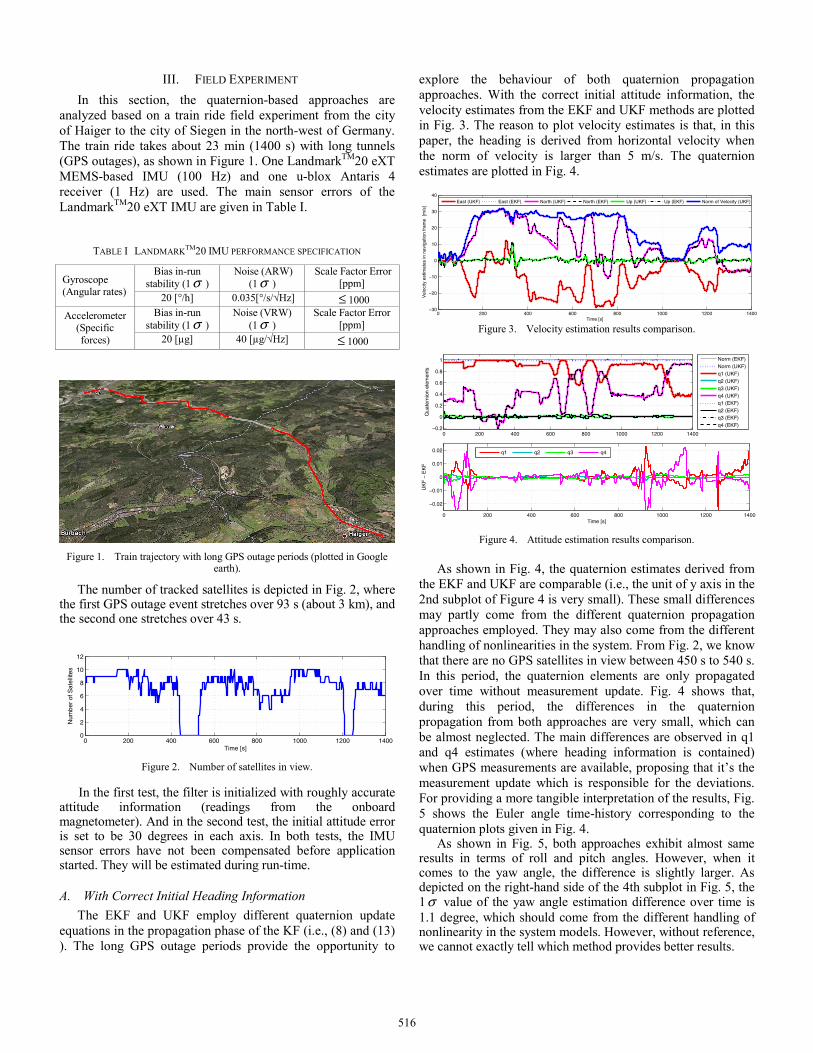
III. FIELD EXPERIMENT In this section, the quaternion-based approaches are

analyzed based on a train ride field experiment from the city of Haiger to the city of Siegen in the north-west of Germany. The train ride takes about 23 min (1400 s) with long tunnels (GPS outages), as shown in Figure 1. One LandmarkTM20 eXT MEMS-based IMU (100 Hz) and one u-blox Antaris 4 receiver (1 Hz) are used. The main sensor errors of the LandmarkTM20 eXT IMU are given in Table I.

TABLE I LANDMARKTM20 IMU PERFORMANCE SPECIFICATION

Gyroscope (Angular rates)

Bias in-run stability (1σ )

Noise (ARW) (1σ )

Scale Factor Error [ppm]

20 [°/h] 0.035[°/s/√Hz] ≤ 1000 Accelerometer

(Specific forces)

Bias in-run stability (1σ )

Noise (VRW) (1σ )

Scale Factor Error [ppm]

20 [µg] 40 [µg/√Hz] ≤ 1000

Figure 1. Train trajectory with long GPS outage periods (plotted in Google

earth).

The number of tracked satellites is depicted in Fig. 2, where the first GPS outage event stretches over 93 s (about 3 km), and the second one stretches over 43 s.

0 200 400 600 800 1000 1200 14000

2

4

6

8

10

12

Time [s]

Num

ber

of S

atel

lites

Figure 2. Number of satellites in view.

In the first test, the filter is initialized with roughly accurate attitude information (readings from the onboard magnetometer). And in the second test, the initial attitude error is set to be 30 degrees in each axis. In both tests, the IMU sensor errors have not been compensated before application started. They will be estimated during run-time.

A. With Correct Initial Heading Information The EKF and UKF employ different quaternion update

equations in the propagation phase of the KF (i.e., (8) and (13)). The long GPS outage periods provide the opportunity to

explore the behaviour of both quaternion propagation approaches. With the correct initial attitude information, the velocity estimates from the EKF and UKF methods are plotted in Fig. 3. The reason to plot velocity estimates is that, in this paper, the heading is derived from horizontal velocity when the norm of velocity is larger than 5 m/s. The quaternion estimates are plotted in Fig. 4.

0 200 400 600 800 1000 1200 1400−30

−20

−10

0

10

20

30

40

Vel

ocity

est

imat

es in

nav

igat

ion

fram

e [m

/s]

Time [s]

East (UKF) East (EKF) North (UKF) North (EKF) Up (UKF) Up (EKF) Norm of Velocity (UKF)

Figure 3. Velocity estimation results comparison.

0 200 400 600 800 1000 1200 1400−0.2

0

0.2

0.4

0.6

0.8

1

Qua

tern

ion

elem

ents

0 200 400 600 800 1000 1200 1400

−0.02

−0.01

0

0.01

0.02

Time [s]

UK

F −

EK

F

q1 q2 q3 q4

Norm (EKF) Norm (UKF)q1 (UKF)q2 (UKF)q3 (UKF)q4 (UKF)q1 (EKF)q2 (EKF)q3 (EKF)q4 (EKF)

Figure 4. Attitude estimation results comparison.

As shown in Fig. 4, the quaternion estimates derived from

the EKF and UKF are comparable (i.e., the unit of y axis in the 2nd subplot of Figure 4 is very small). These small differences may partly come from the different quaternion propagation approaches employed. They may also come from the different handling of nonlinearities in the system. From Fig. 2, we know that there are no GPS satellites in view between 450 s to 540 s. In this period, the quaternion elements are only propagated over time without measurement update. Fig. 4 shows that, during this period, the differences in the quaternion propagation from both approaches are very small, which can be almost neglected. The main differences are observed in q1 and q4 estimates (where heading information is contained) when GPS measurements are available, proposing that it’s the measurement update which is responsible for the deviations. For providing a more tangible interpretation of the results, Fig. 5 shows the Euler angle time-history corresponding to the quaternion plots given in Fig. 4.

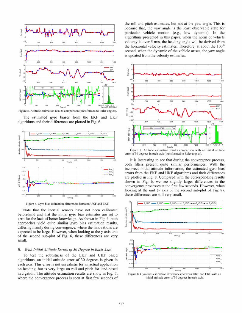
As shown in Fig. 5, both approaches exhibit almost same results in terms of roll and pitch angles. However, when it comes to the yaw angle, the difference is slightly larger. As depicted on the right-hand side of the 4th subplot in Fig. 5, the 1σ value of the yaw angle estimation difference over time is 1.1 degree, which should come from the different handling of nonlinearity in the system models. However, without reference, we cannot exactly tell which method provides better results.

516

0 200 400 600 800 1000 1200 1400−10

−5

0

5

10

Rol

l [de

g]

0 200 400 600 800 1000 1200 1400−10

−5

0

5

Pitc

h [d

eg]

0 200 400 600 800 1000 1200 1400−150

−100

−50

0

50

Yaw

[deg

]

0 200 400 600 800 1000 1200 1400−1

−0.5

0

0.5

1

UK

F−

EK

F [d

eg]

Time [s]

−3 −1.1 0 1.1 30

1

2

3

4

5x 10

4

Yaw (UKF−EKF) [deg]

Roll Pitch Yaw

UKFEKF

Figure 5. Attitude estimation results comparison (transformed to Euler angles).

The estimated gyro biases from the EKF and UKF algorithms and their differences are plotted in Fig. 6.

0 200 400 600 800 1000 1200 1400−0.2

−0.1

0

0.1

Time [s]

Gyr

o bi

as e

stim

ates

[deg

/s]

G

x (UKF) G

y (UKF) G

z (UKF) G

x (EKF) G

y (EKF) G

z (EKF)

0 200 400 600 800 1000 1200 1400−0.015

−0.01

−0.005

0

0.005

0.01

0.015

0.02

UK

F−E

KF

[deg

/s]

Time [s]

Gyro

x

Gyroy

Gyroz

Figure 6. Gyro bias estimation differences between UKF and EKF.

Note that the inertial sensors have not been calibrated beforehand and that the initial gyro bias estimates are set to zero for the lack of better knowledge. As shown in Fig. 6, both approaches yield quite similar gyro bias estimation results, differing mainly during convergence, where the innovations are expected to be large. However, when looking at the y axis unit of the second sub-plot of Fig. 6, these differences are very small.

B. With Initial Attitude Errors of 30 Degree in Each Axis To test the robustness of the EKF and UKF based

algorithms, an initial attitude error of 30 degrees is given in each axis. This error is not unrealistic for an actual application on heading, but is very large on roll and pitch for land-based navigation. The attitude estimation results are show in Fig. 7, where the convergence process is seen at first few seconds of

the roll and pitch estimates, but not at the yaw angle. This is because that, the yaw angle is the least observable state for particular vehicle motion (e.g., low dynamic). In the algorithms presented in this paper, when the norm of vehicle velocity is over 5 m/s, the heading angle will be derived from the horizontal velocity estimates. Therefore, at about the 100th second, when the dynamic of the vehicle arises, the yaw angle is updated from the velocity estimates.

0 200 400 600 800 1000 1200 1400−20

0

20

40

Rol

l [de

g]

0 200 400 600 800 1000 1200 1400−10

0

10

20

30

Pitc

h [d

eg]

0 200 400 600 800 1000 1200 1400−150

−100

−50

0

50

Yaw

[deg

]

0 200 400 600 800 1000 1200 1400−2

−1

0

1

2

UK

F−

EK

F [d

eg]

Time [s]

−3 −1.1 0 1.1 30

2

4

6

x 104

UKFEKF

Roll Pitch Yaw

Figure 7. Attitude estimation results comparison with an initial attitude

error of 30 degrees in each axis (transformed to Euler angles).

It is interesting to see that during the convergence process, both filters present quite similar performances. With the incorrect initial attitude information, the estimated gyro bias errors from the EKF and UKF algorithms and their differences are plotted in Fig. 8. Compared with the corresponding results shown in Fig. 6, we see slightly larger differences in the convergence processes at the first few seconds. However, when looking at the unit (y axis of the second sub-plot of Fig. 8), these differences are still very small.

200 400 600 800 1000 1200 1400−0.2

−0.1

0

0.1

Time [s]

Gyr

o bi

as e

stim

ates

[deg

/s]

G

x (UKF) G

y (UKF) G

z (UKF) G

x (EKF) G

y (EKF) G

z (EKF)

0 200 400 600 800 1000 1200 1400−0.025

−0.02

−0.015

−0.01

−0.005

0

0.005

0.01

UK

F−

EK

F [d

eg/s

]

Time [s]

Gyrox

Gyroy

Gyroz

Figure 8. Gyro bias estimation differences between UKF and EKF with an

initial attitude error of 30 degrees in each axis.

517

The reason why both approaches show similar convergence performances even when the initial attitude errors are set to be 30 degrees could because that, using the quaternion as the representation of attitude, the direction cosine matrix does not feature trigonometric operations, which reduce nonlinearity problems compared to the Euler angle-based approach. Performances from the Euler-angle based approaches can be found in [22-24].

On the processing load, the EKF requires a significantly lower computational burden (about 40% of the UKF approach). This processing time is evaluated using Matlab programming, which cannot be considered as a direct measure of the exact computational burden. For the knowledge on the exact processing load, usually, the number of multiplications and additions should be counted separately, as the way done in [25-26]. It is also worth mentioning that for any KF-based integration approach, correct tuning of the filter covariance parameters is crucial. A variation of these parameters may significantly change the system estimation performance. In order to prevent this problem, the same set of covariance parameters is applied to both methods throughout the results presented in this article.

IV. CONCLUSION In this contribution, the system performances of a tightly-

coupled INS/GPS system using quaternion-based EKF and UKF algorithms are analyzed. A train ride field experiment is evaluated. Numerical results show that both approaches yield comparable attitude and bias estimation accuracy. The different ways of propagating the quaternion vector over time do not imply a difference. The UKF should principally handle the nonlinear nature of the problem, and quaternion propagation in a more accurate manner. However, we do not see much difference with respect to the EKF results, even when the initial attitude errors are set to be 30 degrees in each axis.

ACKNOWLEDGMENT The first author gratefully acknowledges the support

provided by the Multi Modal Sensor Systems for Environmental Exploration and Safety (MOSES) from Center for Sensorsystems (ZESS) in University of Siegen, Germany.

REFERENCES [1] O. Loffeld, Estimationstheorie I + II. München: Oldenbourg Verlag,

1990. [2] R. G. Brown and P. Y. C. Hwang, Introduction to Random signals and

Applied Kalman Filtering, 3 ed. New York: John Wiley & Sons, 1997. [3] P. S. Maybeck, Stochastic Models, Estimation and Control vol. 1. New

York: Academic Press Inc., 1979. [4] D. Lerro and Y. Bar-Shalom, "Tracking with debiased consistent

converted measurements versus EKF," IEEE Trans. on Aerospace and Electronic Systems, vol. 29, pp. 1015 - 1022, 1993.

[5] J. L. Crassidis, "Sigma-Point Kalman Filtering for Integrated GPS and Inertial Navigation," in AIAA Guidance, Navigation, and Control Conference, San Francisco, California, 2005.

[6] S. J. Julier and J. K. Uhlmann, "Unscented filtering and nonlinear estimation," IEEE Review, vol. 92, pp. 401 - 422, 2004.

[7] S. J. Julier, J. K. Uhlmann, and H. F. Durrant-Whyte, "A new method for the nonlinear transformation of means and covariances in filters and estimators," IEEE Trans. on Automatic Control, vol. 45, pp. 477 - 482, 2000.

[8] S. J. Julier and J. K. Uhlmann, "A Consistent, Debiased Method for Converting Between Polar and Cartesian Coordinate Systems," in AeroSense: Acquisition, Tracking and Pointing XI, Orlando FL, 1997, pp. 110–121.

[9] A. Farrell, Aided Navigation: GPS with High Rate Sensors. New York: Mcgraw-Hill Professional, 2008.

[10] E.-H. Shin, X. Niu, and N. El-Sheimy, "Performance Comparison of the Extended and the Unscented Kalman Filter for Integrated GPS and MEMS-Based Inertial Systems," in ION NTM 2005, San Diego, CA, 2005, pp. 961-969.

[11] E.-H. Shin, "A Quaternion-Based Unscented Kalman Filter for the Integration of GPS and MEMS INS," in ION GNSS 2004, Long Beach, CA, 2004, pp. 1060-1068.

[12] E.-H. Shin and N. El-Sheimy, "Unscented Kalman Filter and Attitude Errors of Low-cost Inertial Navigation Systems," NAVIGATION, vol. 54, pp. 1-9, 2007.

[13] W. Khoder, B. Fassinut-Mombot, and M. Benjelloun, "Quaternion Unscented Kalman Filtering for integrated Inertial Navigation and GPS," in 11th International Conference on Information Fusion, 2008 Cologne, Germany, 2008.

[14] E. J. Lefferts, F. L. Markley, and M. D. Schuster, "Kalman Filtering for Spacecraft Attitude Estimation," Journal of Guidance, Control, and Dynamics, vol. 5, pp. 417-429, 1982.

[15] S. Hong, M. H. Lee, H.-H. Chun, S.-H. Kwon, and J. L. Speyer, "Observability of error States in GPS/INS integration," IEEE Trans. on Vehicular Technology, vol. 54, pp. 731 - 743, 2005.

[16] J. T. W. Ryley, P. M. G. Silson, A. Tsourdos, and S. Jordan, "Observability of a stationary GPS aided INS," in AIAA Guidance, Navigation, and Control Conference, Toronto, Ontario, 2010.

[17] I. Rhee, M. F. Abdel-Hafez, and J. L. Speyer, "Observability of an integrated GPS/INS during maneuvers," IEEE Trans. on Aerospace and Electronic Systems, vol. 40, pp. 526 - 535, 2004.

[18] W. R. Hamilton, Elements of Quaternions. London, England: Longmans, green and Co., 1866.

[19] S. Sukkarieh, E. M. Nebot, and H. F. Durrant-Whyte, "A High Integrity IMU/GPS Navigation Loop for Autonomous Land Vehicle Applications," IEEE Trans. on Robotics and Automation, vol. 15, pp. 572-578, 1999.

[20] D. H. Titterton and J. L. Weston, Strapdown Inertial Navigation Technology, 2 ed.: The institution of Electrical Engineers, 2004.

[21] D. Simon, Optimal State Estimation: Kalman, H Infinity, and Nonlinear Approaches, 1 ed. New Jersey: John Wiley & Sons, 2006.

[22] J. Zhou, E. Edwan, S. Knedlik, and O. Loffeld, "Low-cost INS/GPS with nonlinear filtering methods," in FUSION, Edinburgh, 2010.

[23] J. Zhou, Y. Yang, J. Zhang, E. Edwan, "Applying Quaternion-based Unscented Particle Filter on INS/GPS with Field Experiments", Proceedings of the 24th International Technical Meeting of The Satellite Division of the Institute of Navigation (ION GNSS 2011), Portland, Oregon, September 20 - 23, 2011.

[24] J. Zhou, S. Knedlik, O. Loffeld, "INS/GPS tightly-coupled integration using adaptive unscented particle filter", The Journal of Navigation (Royal Institute of Navigation), Vol. 63, no. 3, pp. 491-513, 2010.

[25] J. Zhou, S. Knedlik, O. Loffeld, "Sequential Processing of Integrated Measurements in Tightly-coupled INS/GPS Integrated Navigation System", AIAA Guidance, Navigation and Control, Toronto, Ontario, Canada, 2-5 August 2010.

[26] J. Zhou, S. Knedlik, and O. Loffeld, "INS/GPS for High-Dynamic UAV-Based Applications," International Journal of Navigation and Observation, vol. 2012, 2012.

518