Energy Conversion and Management 65 (2013) 397–407

Contents lists available at SciVerse ScienceDirect

Energy Conversion and Management

journal homepage: www.elsevier .com/ locate /enconman

Incremental artificial bee colony with local search to economic dispatch problemwith ramp rate limits and prohibited operating zones

Serdar Özyön a,⇑, Dogan Aydin b

a Electrical and Electronics Engineering Department, Dumlupınar University, 43100 Kütahya, Turkeyb Computer Engineering Department, Dumlupınar University, 43100 Kütahya, Turkey

a r t i c l e i n f o a b s t r a c t

Article history:Received 22 December 2011Received in revised form 6 July 2012Accepted 6 July 2012Available online 17 October 2012

Keywords:Economic power dispatchProhibited operating zonesRamp rate limitsIncremental artificial bee colony algorithmLocal search

0196-8904/$ - see front matter � 2012 Elsevier Ltd. Ahttp://dx.doi.org/10.1016/j.enconman.2012.07.005

⇑ Corresponding author. Tel.: +90 274 265 2031/42E-mail addresses: serdarozyon@dpu.edu.tr (S. Özy

(D. Aydin).

In this study, prohibited operating zone economic power dispatch problem which considers ramp ratelimit, has been solved by incremental artificial bee colony algorithm (IABC) and incremental artificialbee colony algorithm with local search (IABC-LS) methods. The transmission line losses used in the solu-tion of the problem have been computed by B-loss matrix. IABC, IABC-LS methods have been applied tothree different test systems in literature which consist of 6, 15 and 40 generators. The attained optimumsolution values have been compared with the optimum results in literature and have been discussed.

� 2012 Elsevier Ltd. All rights reserved.

1. Introduction

Today along with an increase in the need for electrical energy,economic power dispatch problem has become one of the mostimportant issues in the operation of power systems. Economicpower dispatch problem is known as the meeting of the presentload in the system by the generation units under system limits withthe minimum total fuel cost. In the solution of this kind of problems,the solution of the problems are simplified by ignoring some limitssuch as ramp rate limits belonging to generators and prohibitedoperating zones. These kinds of problems are known as simplifiedeconomic power dispatch problems partially carrying the character-istics of the real problems. Therefore, with the addition of theaforementioned limits economic power dispatch problems becomemuch closer to real problems. In this way, economic power dispatchproblems with additional limits are transformed to non-linear opti-mization problems with more limits. The economic power dispatchproblem with prohibited operating zone is a nonlinear problem theoptimum solution of which is rather difficult to find [1].

In the literature search, particle swarm optimization, improvedparticle swarm optimization and hybrid particle swarm optimiza-tion algorithms (NAPSO [1], FAPSO [1], MPSO [2], GCPSO [2], IPSO[3], PSO-LRS [4], NPSO [4], NPSO-LRS [4], PSO [5], APSO [6], SOH_P-SO [7], DSPSO-TSA [8], SA-PSO [9], CTPSO [10], CPSO [11], TVAC-

ll rights reserved.

64; fax: +90 274 265 2066.ön), dogan.aydin@dpu.edu.tr

IPSO [12], QPSO [13], QPSO-DM [13], PSO-TVAC [14]), honey beemating optimization and improved honey bee mating optimizationalgorithms (HBMO [15], IHBMO [15]), genetic, improved geneticand hybrid genetic algorithms (GA [16], SSGA [17], GA-MU [18],IGAMU [18], RCGA [19], GA-API [20]) approaches, evolutionaryprogramming, fast computation evolutionary programming andimproved evolutionary programming algorithms (EP [22], QEA[23], IQEA [23], CEP [24], FEP [24], MFEP [24], IFEP [24], ETQ[25], ESO [26]), mixed integer quadratic programming approach(MIQP [27]), artificial immune system optimization algorithm(AIS [28]), biogeography-based optimization and oppositional bio-geography-based optimization algorithms (BBO [29], OBBO [30]),simulated annealing approach (SA [31]), tabu search and multipletabu search algorithms (TS [31], MTS[31]), enhanced direct searchapproach (EDSA [32]), differential evolution, modified differentialevolution and hybrid differential evolution algorithms (DE [33],MDE [34], HDE [35]), harmony search and hybrid harmony searchalgorithms (HS [36], HHS [36]), artificial bee colony optimizationmethod (ABC [37]) civilized swarm and society-civilization optimi-zation algorithm (CSO [38], SCA [38]), effortless hybrid method(EHM [39]), shuffle frog leaping and hybrid shuffle frog leapingoptimization algorithms (SFLA [40], SFLA-SA [40]), bacterial forag-ing optimization with Nelder–Mead hybrid algorithm (BF-NM[41]) and firefly optimization algorithm (FA [42]) have been ap-plied to nonlinear economic power dispatch problems with prohib-ited operating zone.

In this study, for the solution of the economic power dispatchproblem with prohibited operating zone, incremental artificial

398 S. Özyön, D. Aydin / Energy Conversion and Management 65 (2013) 397–407

bee colony optimization (IABC) and incremental artificial bee col-ony optimization with local search algorithms (IABC-LS) have beenused. In the present study for the first time IABC and IABC-LS algo-rithms have been applied to economic power dispatch problemwith prohibited operating zones. In order to define the parametersbelonging to IABC and IABC-LS algorithms Iterated F-Race methodhas been used. IABC and IABC-LS algorithms are based on the prin-ciple of increase in population number during the process. Sociallearning is aimed to be realized in the algorithms.

2. Formulation of the problem

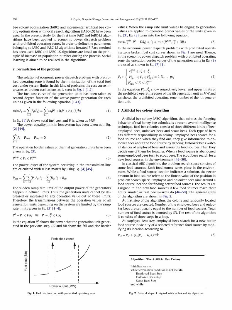
The solution of economic power dispatch problem with prohib-ited operating zone is found by the minimization of the total fuelcost under system limits. In this kind of problems the cost curve in-creases as broken oscillations as is seen in Fig. 1 [1,2].

The fuel cost curve of the generation units has been taken assecond degree function of the active power generation for eachunit as given in the following equation [1,43].

min FT ¼Xn

i¼1

FiðPiÞ ¼Xn

i¼1

ðaiP2i þ biPi þ ciÞ; ð$=hÞ ð1Þ

In Eq. (1) FT shows total fuel cost and Pi is taken as MW.The power equality limit in loss system has been taken as in Eq.

(2) [44].

Xn

i¼1

Pi � Pload � Ploss ¼ 0 ð2Þ

The operation border values of thermal generation units have beengiven in Eq. (3).

Pmini 6 Pi 6 Pmax

i ð3Þ

The power losses of the system occurring in the transmission lineare calculated with B loss matrix by using Eq. (4) [45].

Ploss ¼Xn

i¼1

Xn

j¼1

Pi:Bij:Pj þXn

i¼1

B0i:Pi þ B00 ð4Þ

The sudden ramp rate limit of the output power of the generatorshappen in defined limits. Thus, the generation units cannot be de-creased or increased to any operation value out of these limits.Therefore, the transmissions between the operation values of allgeneration units depending on the system are limited by the ramprate limits given in Eq. (5) [1–4].

P0i � Pi 6 DRi ve Pi � P0

i 6 URi ð5Þ

In the equation P0i shows the power that the generation unit gener-

ated in the previous step, DR and UR show the fall and rise border

Fuel

cos

t ($/

h)

Power output (MW)

Prohibited zones

Fig. 1. Fuel cost function with prohibited operating zone.

values. When the ramp rate limit values belonging to generationvalues are applied to operation border values of the units given inEq. (3), Eq. (3) turns into the following equation.

maxðPmini ; P0

i � DRiÞ 6 Pi 6 minðPmaxi ; P0

i þ URiÞ ð6Þ

In the economic power dispatch problems with prohibited operat-ing zone broken fuel cost curves shown in Fig. 1 are used. Thence,in the economic power dispatch problem with prohibited operatingzone the operation border values of the generation units in Eq. (3)are used as shown in Eq. (7) [1].

Pi 2Pmin

i 6 Pi 6 Pli;1

Pui;j�1 6 Pi 6 Pl

i;j

Pui;pzi6 Pi 6 Pmax

i

8>><>>:

j ¼ 2;3; . . . ;pzi ð7Þ

In the equation Pui;j, Pl

i;j show respectively lower and upper limits ofthe prohibited operating zones of the ith generation unit as MW andpzi shows the prohibited operating zone number of the ith genera-tion unit.

3. Artificial bee colony algorithm

Artificial bee colony (ABC) algorithm, that mimics the foragingbehavior of real honey bee colonies, is a recent swarm intelligencetechnique. Real bee colonies consist of three different kinds of bee:employed bees, onlooker bees and scout bees. Each type of beeshas different responsibility in colony. Employed bees search for afood source and when they find one, they give information to on-looker bees about the food source by dancing. Onlooker bees watchall dances of employed bees and assess the food sources. Then theydecide one of them for foraging. When a food source is abandonedsome employed bees turn to scout bees. The scout bees search for anew food sources in the environment [46–50].

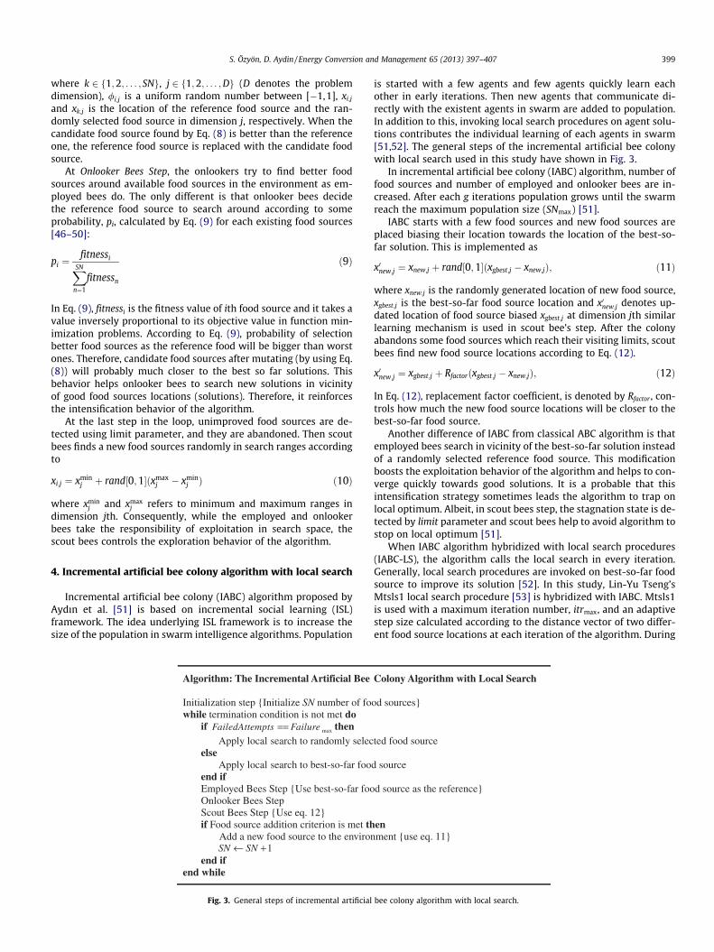
In classical ABC algorithm, the problem search space consists ofsome food sources. Each food source takes place in the environ-ment. While a food source location indicates a solution, the nectaramount in food source refers to the fitness value of the position inproblem search space. Employed and onlooker bees look around afood source location for finding better food sources. The scouts areassigned to find new food sources if few food sources reach theirlimits similar as real bee swarms do [46–50]. The general stepsof the algorithm are shown in Fig. 2.

At first step of the algorithm, the colony and randomly locatedfood sources are created. Number of the employed bees and onloo-ker bees are set usually equal to the number of food sources. Totalnumber of food source is denoted by SN. The rest of the algorithmis consists of three steps in a loop.

At employed bees step, employed bees search for a new betterfood source in vicinity of a selected reference food source by mod-ifying its location according to

v i;j ¼ xi;j þ /i;jðxi;j � xk;jÞ; i–k ð8Þ

Algorithm: The Artificial Bee Colony

Initialization stepwhile termination condition is not met do

Employed Bees StepOnlooker Bees StepScout Bees Step

end while

Fig. 2. General steps of original artificial bee colony algorithm.

S. Özyön, D. Aydin / Energy Conversion and Management 65 (2013) 397–407 399

where k 2 f1;2; . . . ; SNg, j 2 f1;2; . . . ;Dg (D denotes the problemdimension), /i;j is a uniform random number between [�1,1], xi;j

and xk;j is the location of the reference food source and the ran-domly selected food source in dimension j, respectively. When thecandidate food source found by Eq. (8) is better than the referenceone, the reference food source is replaced with the candidate foodsource.

At Onlooker Bees Step, the onlookers try to find better foodsources around available food sources in the environment as em-ployed bees do. The only different is that onlooker bees decidethe reference food source to search around according to someprobability, pi, calculated by Eq. (9) for each existing food sources[46–50]:

pi ¼fitnessi

XSN

n¼1

fitnessn

ð9Þ

In Eq. (9), fitnessi is the fitness value of ith food source and it takes avalue inversely proportional to its objective value in function min-imization problems. According to Eq. (9), probability of selectionbetter food sources as the reference food will be bigger than worstones. Therefore, candidate food sources after mutating (by using Eq.(8)) will probably much closer to the best so far solutions. Thisbehavior helps onlooker bees to search new solutions in vicinityof good food sources locations (solutions). Therefore, it reinforcesthe intensification behavior of the algorithm.

At the last step in the loop, unimproved food sources are de-tected using limit parameter, and they are abandoned. Then scoutbees finds a new food sources randomly in search ranges accordingto

xi;j ¼ xminj þ rand½0;1�ðxmax

j � xminj Þ ð10Þ

where xminj and xmax

j refers to minimum and maximum ranges indimension jth. Consequently, while the employed and onlookerbees take the responsibility of exploitation in search space, thescout bees controls the exploration behavior of the algorithm.

4. Incremental artificial bee colony algorithm with local search

Incremental artificial bee colony (IABC) algorithm proposed byAydın et al. [51] is based on incremental social learning (ISL)framework. The idea underlying ISL framework is to increase thesize of the population in swarm intelligence algorithms. Population

Algorithm: The Incremental Artificial Bee

Initialization step {Initialize SN number of fowhile termination condition is not met do

if maxFailedAttempts Failure== then Apply local search to randomly selec

else Apply local search to best-so-far foo

end if Employed Bees Step {Use best-so-far foo Onlooker Bees Step Scout Bees Step {Use eq. 12}

if Food source addition criterion is met thAdd a new food source to the environ

1SN SN← +end if

end while

Fig. 3. General steps of incremental artificial

is started with a few agents and few agents quickly learn eachother in early iterations. Then new agents that communicate di-rectly with the existent agents in swarm are added to population.In addition to this, invoking local search procedures on agent solu-tions contributes the individual learning of each agents in swarm[51,52]. The general steps of the incremental artificial bee colonywith local search used in this study have shown in Fig. 3.

In incremental artificial bee colony (IABC) algorithm, number offood sources and number of employed and onlooker bees are in-creased. After each g iterations population grows until the swarmreach the maximum population size (SNmax) [51].

IABC starts with a few food sources and new food sources areplaced biasing their location towards the location of the best-so-far solution. This is implemented as

x0new;j ¼ xnew;j þ rand½0;1�ðxgbest;j � xnew;jÞ; ð11Þ

where xnew;j is the randomly generated location of new food source,xgbest;j is the best-so-far food source location and x0new;j denotes up-dated location of food source biased xgbest;j at dimension jth similarlearning mechanism is used in scout bee’s step. After the colonyabandons some food sources which reach their visiting limits, scoutbees find new food source locations according to Eq. (12).

x0new;j ¼ xgbest;j þ Rfactorðxgbest;j � xnew;jÞ; ð12Þ

In Eq. (12), replacement factor coefficient, is denoted by Rfactor , con-trols how much the new food source locations will be closer to thebest-so-far food source.

Another difference of IABC from classical ABC algorithm is thatemployed bees search in vicinity of the best-so-far solution insteadof a randomly selected reference food source. This modificationboosts the exploitation behavior of the algorithm and helps to con-verge quickly towards good solutions. It is a probable that thisintensification strategy sometimes leads the algorithm to trap onlocal optimum. Albeit, in scout bees step, the stagnation state is de-tected by limit parameter and scout bees help to avoid algorithm tostop on local optimum [51].

When IABC algorithm hybridized with local search procedures(IABC-LS), the algorithm calls the local search in every iteration.Generally, local search procedures are invoked on best-so-far foodsource to improve its solution [52]. In this study, Lin-Yu Tseng’sMtsls1 local search procedure [53] is hybridized with IABC. Mtsls1is used with a maximum iteration number, itrmax, and an adaptivestep size calculated according to the distance vector of two differ-ent food source locations at each iteration of the algorithm. During

Colony Algorithm with Local Search

od sources}

ted food source

d source

d source as the reference}

enment {use eq. 11}

bee colony algorithm with local search.

400 S. Özyön, D. Aydin / Energy Conversion and Management 65 (2013) 397–407

algorithm in progress, the difference between any two food sourcelocation decreases and step size for Mtsls1 too. Thus, diversifica-tion behavior is boosted in early iterations of the IABC-LS, thendiversification of the algorithm is increased in later iterations [54].

In ABC-LS, we generated a mechanism for fighting stagnation. Iflocal search calls cannot improve the results after a maximumnumber of repeated calls (Failuresmax) the local search proceduresare applied to a randomly selected location. Furthermore, boundconstraints are not checked in classic Mtsls1. The following penaltyfunction is used for boundary constraint satisfaction [50,51,54]:

PðxÞ ¼ fes�XD

j¼1

BoundðxiÞ ð13Þ

In Eq. (13) fes refers to the number of function evaluations that havebeen used so far.

BoundðxiÞ ¼

0; if xmaxj > xj > xmin

j

ðxminj � xjÞ2; if xj < xmin

j

ðxmaxj � xjÞ2; if xj > xmax

j

8>><>>:

ð14Þ

Table 1The best parameter values of IABC and IABC-LS obtained by Iterated F-Race.

Algorithm SN Limit SNmax g Rfactor itrmax Failuresmax

Ranges [3,20] (1,100] (20,100] [1,10] (10�8,1) (1,200) (1,20)IABC 9 98 15 8 10�0.94 – –IABC-LS 5 11 88 6 10�0.94 192 19

4.1. Application IABC and IABC-LS algorithms to the problem

In this subsection, it is explained that how IABC and IABC-LS areused for economic dispatch problem with ramp rate limits andprohibited operating zones.

Before generating population, minimum and maximum poweroutputs of generation units are updated by using Eq. (6) accordingto P0

i , ramp up/down rate limits. Then population is created takingminimum and maximum power outputs of generation units intoaccount. For SN number of food sources, Pi values are calculatedfor ensuring equality in Eq. (3) by using following Eq. (15):

Pi ¼ Pmini þ rand½0;1� � ðPmax

i � Pmini Þ ; i 2 f1;2; . . . ; SNg ð15Þ

In equation, Pmini and Pmax

i are minimum and maximum power out-puts of ith generation unit updated by using Eq. (6). When a newfood source is added after each g iterations, the created Pnew valueusing Eq. (15) is updated considering Eq. (11) as the following:

P0new ¼ Pnew þ rand½0;1�ðPgbest � PnewÞ ð16Þ

where Pgbest refers to best food source location and P0new denotes up-dated location of food source.

Satisfaction of active power balance constraint given in Eq. (2) isvery important in swarm creation. To enforce active power equa-tion, lth dependent generator (slack bus), whose generation power,is Pi,l is selected randomly. The value of generation power, Pold

i;l , iscalculated by Eq. (17) where Pold

loss ¼ Pfirstloss ¼ 0 at starting condition:

Poldi;l ¼ Pload þ Ploss �

Xi2NG ;lRNG

Pi ð17Þ

After obtaining Poldi;l , Pnew

loss is determined by Eq. (4). According to this,Pnew

i;l is figured out from the following equation:

Pnewi;l ¼ Pold

i;l þ Pnewloss � Pold

loss ð18Þ

The result of this equation is controlled in Eq. (19) and if the error isbelow error tolerance value the equation satisfies the constraint de-fined in Eq. (3):

Error ¼ jPoldloss � Pold

lossj; Error 6 TOLerror ð19Þ

In this case, the obtained Pnewi;l is checked whether it satisfies the

constraint defined in Eq. (6) or not. If it does not satisfy, the algo-rithm turns back to Eq. (15) and tries the reassignment for the foodsource. If it satisfies, the objective value of the new food source iscalculated using Eq. (1) and the algorithm process continues. In this

paper, the result of Eq. (1) is defined as objective value for the prob-lem. This constraint satisfaction process is used after each functionevaluation (each change in food source locations) in the algorithm.Each created food source by this way contains suitable solutionsthen they are added to the population.

Furthermore, at each iteration of the algorithm, the modifiedfood source locations by bees should satisfy all the constraints de-fined in the problem. To enforce constraints, lower and upperboundaries of power values proposed by food source are updatedusing Eq. (6) according to ramp up/down rate limits. By using thisafter each function call, generation units are prevented to changeout of increasing/decreasing limits. Any power value in the solu-tion of a food source which doesn’t satisfy the constraint is en-forced by the boundary constraints by using following equation:

Pi ¼

Pmini if Pi < Pmin

i

Pli;j if Pl

i;j > Pi << Pui;pzi

Pui;pzi

if Pli;j >> Pi < Pu

i;pzi

Pmaxi if Pi > Pmax

i

8>>>>><>>>>>:

9>>>>>=>>>>>;

j ¼ 2; . . . ;pzi ð20Þ

4.2. Automatic parameter setting with Iterated F-Race

F-Race is used for selecting the best algorithm configuration (aparticular setting of numerical and categorical parameters of analgorithm) from of a set of candidate configurations under stochas-tic evaluations. In F-Race, candidate configurations are evaluatediteratively on a set of problem instances. As soon as sufficient sta-tistical evidence is gathered against a candidate configuration, it isdiscarded from the race. The process continues until a single can-didate configuration is selected, or until the maximum number ofevaluations or instances is reached.

The generation of candidate configurations is independent of F-Race. A method that combines F-Race with a process capable ofgenerating promising candidate configurations is called iteratedF-Race [55,56]. It consists in executing the steps of configurationgeneration, selection and refinement iteratively. For numericalparameters, the configuration generation step involves samplingfrom Gaussian distributions centered at promising solutions andwith standard deviations that vary over time in order to focusthe search around the best-so-far solutions. The process is de-scribed in detail in [55,56].

To use iterated F-Race, one needs to select the parameters to betuned, their range or domain, and the set of instances on whichtuning is to be performed. The set of parameters selected for tuningand their ranges, for both IABC and IABC-LS, are listed in Table 1.Other parameter settings are remained fixed.

Usually, problem instances are fed to F-Race as a stream. Thismeans that candidate configurations ‘‘see’’ different problem in-stances every time they are tested. After each candidate configura-tion in the race has been evaluated, a statistical test is applied inorder to determine whether there are configurations that have,up to that point, performed significantly worse than the others.In our case, it is not simple to generate many problem instances.Therefore, we rely on the test system with six generators. Duringtuning, at each step, candidate configurations are run once onthe test function.

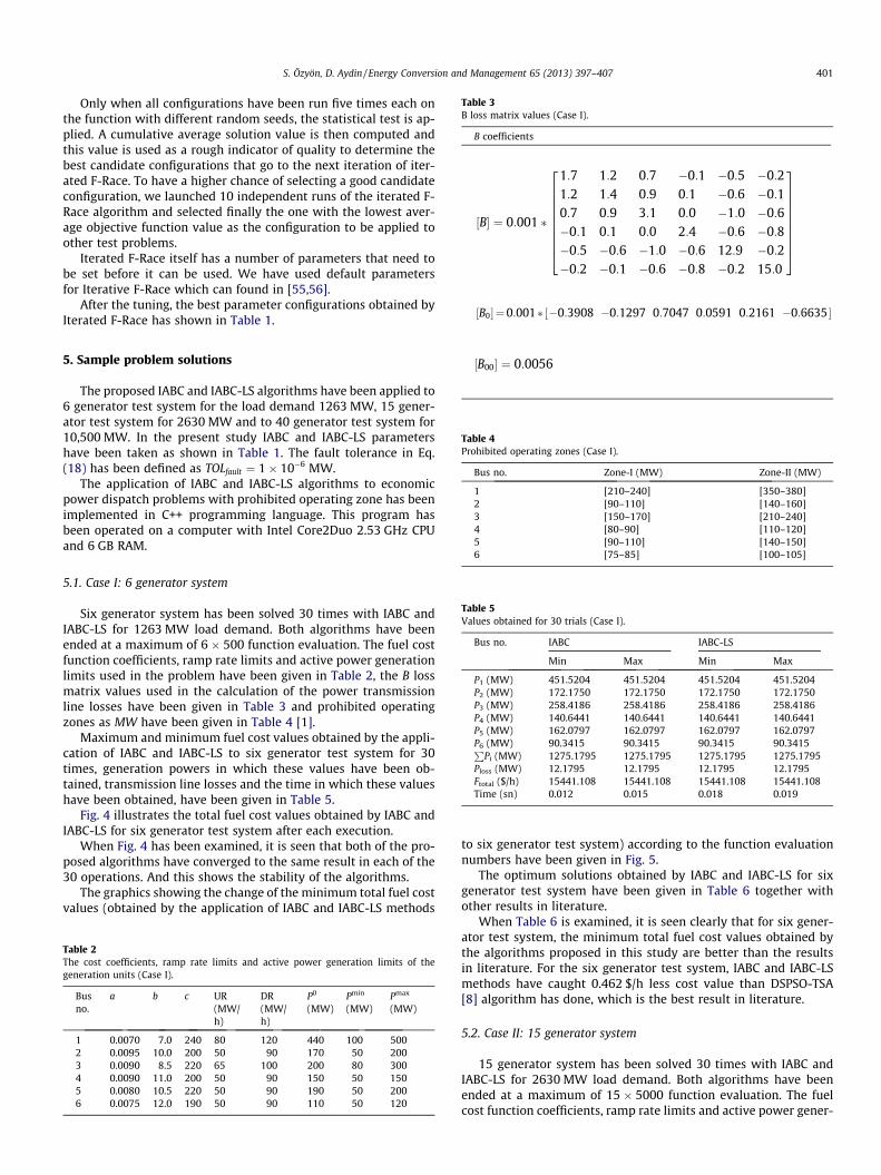
Table 3B loss matrix values (Case I).

B coefficients

½B� ¼ 0:001 �

1:7 1:2 0:7 �0:1 �0:5 �0:21:2 1:4 0:9 0:1 �0:6 �0:10:7 0:9 3:1 0:0 �1:0 �0:6�0:1 0:1 0:0 2:4 �0:6 �0:8�0:5 �0:6 �1:0 �0:6 12:9 �0:2�0:2 �0:1 �0:6 �0:8 �0:2 15:0

2666666664

3777777775

½B0� ¼0:001� �0:3908 �0:1297 0:7047 0:0591 0:2161 �0:6635½ �

S. Özyön, D. Aydin / Energy Conversion and Management 65 (2013) 397–407 401

Only when all configurations have been run five times each onthe function with different random seeds, the statistical test is ap-plied. A cumulative average solution value is then computed andthis value is used as a rough indicator of quality to determine thebest candidate configurations that go to the next iteration of iter-ated F-Race. To have a higher chance of selecting a good candidateconfiguration, we launched 10 independent runs of the iterated F-Race algorithm and selected finally the one with the lowest aver-age objective function value as the configuration to be applied toother test problems.

Iterated F-Race itself has a number of parameters that need tobe set before it can be used. We have used default parametersfor Iterative F-Race which can found in [55,56].

After the tuning, the best parameter configurations obtained byIterated F-Race has shown in Table 1.

½B00� ¼ 0:0056

Table 4Prohibited operating zones (Case I).

Bus no. Zone-I (MW) Zone-II (MW)

1 [210–240] [350–380]2 [90–110] [140–160]3 [150–170] [210–240]4 [80–90] [110–120]5 [90–110] [140–150]

5. Sample problem solutions

The proposed IABC and IABC-LS algorithms have been applied to6 generator test system for the load demand 1263 MW, 15 gener-ator test system for 2630 MW and to 40 generator test system for10,500 MW. In the present study IABC and IABC-LS parametershave been taken as shown in Table 1. The fault tolerance in Eq.(18) has been defined as TOLfault ¼ 1� 10�6 MW.

The application of IABC and IABC-LS algorithms to economicpower dispatch problems with prohibited operating zone has beenimplemented in C++ programming language. This program hasbeen operated on a computer with Intel Core2Duo 2.53 GHz CPUand 6 GB RAM.

6 [75–85] [100–105]

Table 5Values obtained for 30 trials (Case I).

Bus no. IABC IABC-LS

Min Max Min Max

P1 (MW) 451.5204 451.5204 451.5204 451.5204P2 (MW) 172.1750 172.1750 172.1750 172.1750P3 (MW) 258.4186 258.4186 258.4186 258.4186P4 (MW) 140.6441 140.6441 140.6441 140.6441P5 (MW) 162.0797 162.0797 162.0797 162.0797P6 (MW) 90.3415 90.3415 90.3415 90.3415P

Pi (MW) 1275.1795 1275.1795 1275.1795 1275.1795Ploss (MW) 12.1795 12.1795 12.1795 12.1795Ftotal ($/h) 15441.108 15441.108 15441.108 15441.108Time (sn) 0.012 0.015 0.018 0.019

5.1. Case I: 6 generator system

Six generator system has been solved 30 times with IABC andIABC-LS for 1263 MW load demand. Both algorithms have beenended at a maximum of 6 � 500 function evaluation. The fuel costfunction coefficients, ramp rate limits and active power generationlimits used in the problem have been given in Table 2, the B lossmatrix values used in the calculation of the power transmissionline losses have been given in Table 3 and prohibited operatingzones as MW have been given in Table 4 [1].

Maximum and minimum fuel cost values obtained by the appli-cation of IABC and IABC-LS to six generator test system for 30times, generation powers in which these values have been ob-tained, transmission line losses and the time in which these valueshave been obtained, have been given in Table 5.

Fig. 4 illustrates the total fuel cost values obtained by IABC andIABC-LS for six generator test system after each execution.

When Fig. 4 has been examined, it is seen that both of the pro-posed algorithms have converged to the same result in each of the30 operations. And this shows the stability of the algorithms.

The graphics showing the change of the minimum total fuel costvalues (obtained by the application of IABC and IABC-LS methods

Table 2The cost coefficients, ramp rate limits and active power generation limits of thegeneration units (Case I).

Busno.

a b c UR(MW/h)

DR(MW/h)

P0

(MW)Pmin

(MW)Pmax

(MW)

1 0.0070 7.0 240 80 120 440 100 5002 0.0095 10.0 200 50 90 170 50 2003 0.0090 8.5 220 65 100 200 80 3004 0.0090 11.0 200 50 90 150 50 1505 0.0080 10.5 220 50 90 190 50 2006 0.0075 12.0 190 50 90 110 50 120

to six generator test system) according to the function evaluationnumbers have been given in Fig. 5.

The optimum solutions obtained by IABC and IABC-LS for sixgenerator test system have been given in Table 6 together withother results in literature.

When Table 6 is examined, it is seen clearly that for six gener-ator test system, the minimum total fuel cost values obtained bythe algorithms proposed in this study are better than the resultsin literature. For the six generator test system, IABC and IABC-LSmethods have caught 0.462 $/h less cost value than DSPSO-TSA[8] algorithm has done, which is the best result in literature.

5.2. Case II: 15 generator system

15 generator system has been solved 30 times with IABC andIABC-LS for 2630 MW load demand. Both algorithms have beenended at a maximum of 15 � 5000 function evaluation. The fuelcost function coefficients, ramp rate limits and active power gener-

Fig. 4. Total fuel cost values obtained for 30 trials (Case I – IABC and IABC-LS).

Fig. 5. The change of the total fuel cost according to number of function evaluations (Case I – IABC and IABC-LS).

Table 6Results in literature and the optimum solution values obtained by the proposed IABCand IABC-LS (Case I).

Methods Best cost ($/h) Worst cost ($/h) Average cost ($/h)

NAPSO [1] 15443.765664 15443.765683 15443.765671FAPSO [1] 15445.244 15451.63 15448.052MPSO [2] 15443.0925 – –IPSO [3] 15,444 – 15446.3NPSO-LRS [4] 15,450 15,452 15450.5PSO [5] 15,450 15,492 15,454APSO [6] 15449.99 – –SOH-PSO [7] 15446.02 – –TSA [8] 15451.631 15462.263 15506.451DSPSO-TSA [8] 15441.57 15443.84 15446.22SA-PSO [9] 15,447 – –CPSO-1 [11] 15,447 15,490 15,449CPSO-2 [11] 15,446 15,490 15,449QPSO [13] 15442.7717 15467.7765 15446.0042QPSO-DM-1 [13] 15442.6573 15459.0539 15445.6263QPSO-DM-2 [13] 15442.3758 15450.4222 15445.5960GA [16] 15,459 15,524 15,469SSGA [17] 15,447 15,470 15,450GAAPI [20] 15449.78 15449.85 15449.81AIS [28] 15,448 15,472 15459.7BBO [29] 15443.0966 15443.0963 15443.0964OBBO [30] 15442.414 15442.419 15442.415TS [31] 15454.89 15498.05 15472.56MTS [31] 15450.06 15453.64 15451.17SA [31] 15461.10 15545.50 15488.98DE [33] 15449.766 15449.874 15449.777HS [36] 15,449 15,449 15,449HHS [36] 15,449 15,453 15,450EHM [39] 15441.5974 – –BF-NM [41] 15443.8164 – 15446.95383IABC 15441.108 15441.108 15441.108IABC-LS 15441.108 15441.108 15441.108

Table 7The cost coefficients, ramp rate limits and active power generation limits of thegeneration units (Case II).

Busno.

a b c UR(MW/h)

DR(MW/h)

P0

(MW)Pmin

(MW)Pmax

(MW)

1 0.000299 10.1 671 80 120 400 150 4552 0.000183 10.2 574 80 120 300 150 4553 0.001126 8.8 374 130 130 105 20 1304 0.001126 8.8 374 130 130 100 20 1305 0.000205 10.4 461 80 120 90 150 4706 0.000301 10.1 630 80 120 400 135 4607 0.000364 9.8 548 80 120 350 135 4658 0.000338 11.2 227 65 100 95 60 3009 0.000807 11.2 173 60 100 105 25 162

10 0.001203 10.7 175 60 100 110 25 16011 0.003586 10.2 186 80 80 60 20 8012 0.005513 9.9 230 80 80 40 20 8013 0.000371 13.1 225 80 80 30 25 8514 0.001929 12.1 309 55 55 20 15 5515 0.004447 12.4 323 55 55 20 15 55

402 S. Özyön, D. Aydin / Energy Conversion and Management 65 (2013) 397–407

ation limits used in the problem have been given in Table 7, the Bloss matrix values used in the calculation of the power transmis-sion line losses have been given in Table 8 and prohibited opera-tion zones as MW have been given in Table 9 [1]. Total fuel costvalues obtained by IABC and IABC-LS have been shown in Fig. 6.Each point in Fig. 6 indicates a solution value for each execution.

When Fig. 6 is examined, it is seen that although IABC algorithmobtains good results, when it is hybridized with local search proce-dures (IABC-LS) it can escape from local minimum points with a

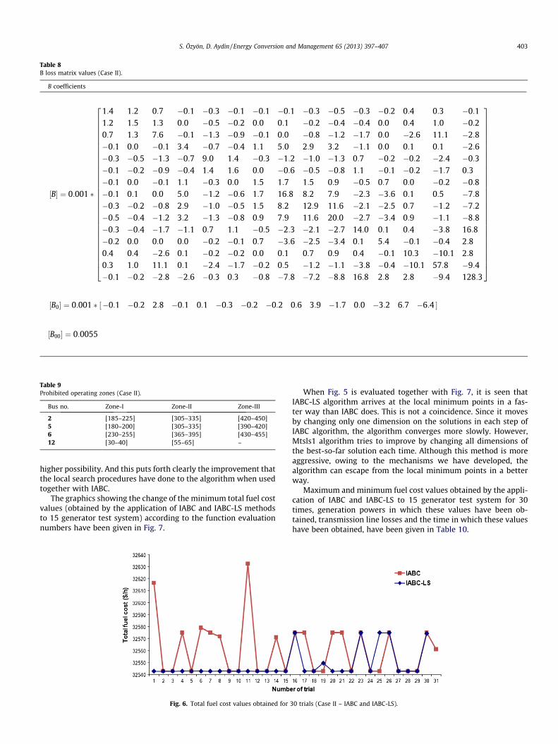
Table 8B loss matrix values (Case II).

B coefficients

½B� ¼ 0:001 �

1:4 1:2 0:7 �0:1 �0:3 �0:1 �0:1 �0:1 �0:3 �0:5 �0:3 �0:2 0:4 0:3 �0:11:2 1:5 1:3 0:0 �0:5 �0:2 0:0 0:1 �0:2 �0:4 �0:4 0:0 0:4 1:0 �0:20:7 1:3 7:6 �0:1 �1:3 �0:9 �0:1 0:0 �0:8 �1:2 �1:7 0:0 �2:6 11:1 �2:8�0:1 0:0 �0:1 3:4 �0:7 �0:4 1:1 5:0 2:9 3:2 �1:1 0:0 0:1 0:1 �2:6�0:3 �0:5 �1:3 �0:7 9:0 1:4 �0:3 �1:2 �1:0 �1:3 0:7 �0:2 �0:2 �2:4 �0:3�0:1 �0:2 �0:9 �0:4 1:4 1:6 0:0 �0:6 �0:5 �0:8 1:1 �0:1 �0:2 �1:7 0:3�0:1 0:0 �0:1 1:1 �0:3 0:0 1:5 1:7 1:5 0:9 �0:5 0:7 0:0 �0:2 �0:8�0:1 0:1 0:0 5:0 �1:2 �0:6 1:7 16:8 8:2 7:9 �2:3 �3:6 0:1 0:5 �7:8�0:3 �0:2 �0:8 2:9 �1:0 �0:5 1:5 8:2 12:9 11:6 �2:1 �2:5 0:7 �1:2 �7:2�0:5 �0:4 �1:2 3:2 �1:3 �0:8 0:9 7:9 11:6 20:0 �2:7 �3:4 0:9 �1:1 �8:8�0:3 �0:4 �1:7 �1:1 0:7 1:1 �0:5 �2:3 �2:1 �2:7 14:0 0:1 0:4 �3:8 16:8�0:2 0:0 0:0 0:0 �0:2 �0:1 0:7 �3:6 �2:5 �3:4 0:1 5:4 �0:1 �0:4 2:80:4 0:4 �2:6 0:1 �0:2 �0:2 0:0 0:1 0:7 0:9 0:4 �0:1 10:3 �10:1 2:80:3 1:0 11:1 0:1 �2:4 �1:7 �0:2 0:5 �1:2 �1:1 �3:8 �0:4 �10:1 57:8 �9:4�0:1 �0:2 �2:8 �2:6 �0:3 0:3 �0:8 �7:8 �7:2 �8:8 16:8 2:8 2:8 �9:4 128:3

266666666666666666666666666666664

377777777777777777777777777777775

½B0� ¼ 0:001 � �0:1 �0:2 2:8 �0:1 0:1 �0:3 �0:2 �0:2 0:6 3:9 �1:7 0:0 �3:2 6:7 �6:4½ �

½B00� ¼ 0:0055

Table 9Prohibited operating zones (Case II).

Bus no. Zone-I Zone-II Zone-III

2 [185–225] [305–335] [420–450]5 [180–200] [305–335] [390–420]6 [230–255] [365–395] [430–455]12 [30–40] [55–65] –

S. Özyön, D. Aydin / Energy Conversion and Management 65 (2013) 397–407 403

higher possibility. And this puts forth clearly the improvement thatthe local search procedures have done to the algorithm when usedtogether with IABC.

The graphics showing the change of the minimum total fuel costvalues (obtained by the application of IABC and IABC-LS methodsto 15 generator test system) according to the function evaluationnumbers have been given in Fig. 7.

Fig. 6. Total fuel cost values obtained for

When Fig. 5 is evaluated together with Fig. 7, it is seen thatIABC-LS algorithm arrives at the local minimum points in a fas-ter way than IABC does. This is not a coincidence. Since it movesby changing only one dimension on the solutions in each step ofIABC algorithm, the algorithm converges more slowly. However,Mtsls1 algorithm tries to improve by changing all dimensions ofthe best-so-far solution each time. Although this method is moreaggressive, owing to the mechanisms we have developed, thealgorithm can escape from the local minimum points in a betterway.

Maximum and minimum fuel cost values obtained by the appli-cation of IABC and IABC-LS to 15 generator test system for 30times, generation powers in which these values have been ob-tained, transmission line losses and the time in which these valueshave been obtained, have been given in Table 10.

30 trials (Case II – IABC and IABC-LS).

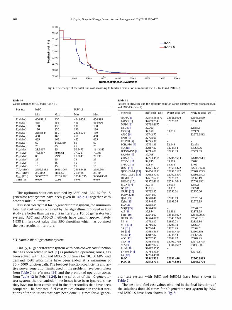
Fig. 7. The change of the total fuel cost according to function evaluation numbers (Case II – IABC and IABC-LS).

Table 10Values obtained for 30 trials (Case II).

Bus no. IABC IABC-LS

Min Max Min Max

P1 (MW) 454.9812 455 454.9859 454.999P2 (MW) 455 455 455 454.996P3 (MW) 130 130 130 130P4 (MW) 130 130 130 130P5 (MW) 235.5844 150 233.8026 150P6 (MW) 460 460 460 460P7 (MW) 465 465 465 465P8 (MW) 60 148.3389 60 60P9 (MW) 25 25 25 25P10 (MW) 28.9867 25 30.5473 111.3145P11 (MW) 76.8357 79.9761 77.0221 79.993P12 (MW) 80 79.99 79.9847 79.999P13 (MW) 25 25 25 25P14 (MW) 15 15 15 15P15 (MW) 15 15 15 15P

Pi (MW) 2656.3882 2658.3067 2656.3428 2656.304Ploss (MW) 26.3882 28.3057 26.3428 26.304Ftotal (R/h) 32542.732 32632.486 32542.735 32574.8361Time (sn) 0.090 0.093 0.078 0.080

Table 11Results in literature and the optimum solution values obtained by the proposed IABCand IABC-LS (Case II).

Methods Best cost ($/h) Worst cost ($/h) Average cost ($/h)

NAPSO [1] 32548.585876 32548.5904 32548.5869FAPSO [1] 32659.794 32676.07 32663.19MPSO [2] 32738.4177 – –IPSO [3] 32,709 – 32784.5PSO [5] 32,858 33,031 32,989APSO [6] 32742.77 – 32976.6812SPSO [7] 32798.69 – –PC_PSO [7] 32775.36 – –SOH_PSO [7] 32751.39 32,945 32,878TSA [8] 32917.87 33245.54 33066.76DSPSO-TSA [8] 32715.06 32730.39 32724.63SA_PSO [9] 32,708 – –CTPSO [10] 32704.4514 32704.4514 32704.4514CPSO-1 [11] 32,835 33,318 33,021CPSO-2 [11] 32,834 33,318 33,021QPSO [13] 32671.4755 32956.6422 32749.8628QPSO-DM-1 [13] 32656.1153 32797.7122 32702.9293QPSO-DM-2 [13] 32652.5750 32767.5801 32695.9502HBMO [15] 32637.6219 32676.07 32663.19IHBMO [15] 32552.4613 32554.6649 32552.8961SSGA [17] 32,711 33,005 32,802GA [20] 33,113 33,337 33,228GAAPI [20] 32732.95 32756.01 32735.06FCEPA [21] 32544.97 – –QEA [23] 32548.48 32806.89 32679.54IQEA [23] 32544.97 32699.56 32575.35ESO [26] 32568.54 – –MIQP [27] 32544.97 – 32544.97AIS [28] 32,854 32,892 32873.25BBO [30] 32544.67 32545.5927 32545.0906OBBO [30] 32544.8670 32545.1749 32545.0101TS [31] 32762.12 32842.71 32822.84MTS [31] 32716.87 32796.13 32767.4

404 S. Özyön, D. Aydin / Energy Conversion and Management 65 (2013) 397–407

The optimum solutions obtained by IABC and IABC-LS for 15generator test system have been given in Table 11 together withother results in literature.

It is seen clearly that for 15 generator test system, the minimumtotal fuel cost values obtained by the algorithms proposed in thisstudy are better than the results in literature. For 30 generator testsystem, IABC and IABC-LS methods have caught approximately1.938 $/h less cost value than BBO algorithm which has obtainedthe best results in literature.

SA [31] 32786.4 33028.95 32869.51DE [33] 32588.865 32641.419 32609.851MDE [34] 32917.87 33245.54 33066.76ABC [37] 32707.85 32708.27 32707.95CSO [38] 32588.9189 32796.7792 32679.8775SCA [38] 32867.025 33381.0607 33138.302EHM [39] 32672.9595 – –BF-NM [41] 32784.5024 – 32976.81FA [42] 32704.4501 – –IABC 32542.732 32632.486 32560.9885IABC-LS 32542.735 32574.8361 32548.3704

5.3. Sample III: 40 generator system

Finally, 40 generator test system with non-convex cost functionthat has been solved in Ref. [1] as prohibited operating zones, hasbeen solved with IABC and IABC-LS 30 times for 10,500 MW loaddemand. Both algorithms have been ended at a maximum of20 � 5000 function calls. The fuel cost function coefficients and ac-tive power generation limits used in the problem have been takenfrom Table 7 in reference [24] and the prohibited operation zonesfrom Table 12 in Refs. [1,24]. In the solution of the 40 generatortest system, the transmission line losses have been ignored, sincethey have not been considered in the other studies that have beencompared. The best total fuel cost values obtained in the last iter-ations of the solutions that have been done 30 times for 40 gener-

ator test system with IABC and IABC-LS have been shown inTable 7.

The best total fuel cost values obtained in the final iterations ofthe solutions done 30 times for 40 generator test system by IABCand IABC-LS have been shown in Fig. 8.

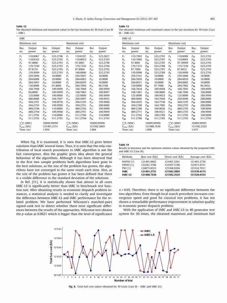
Table 12The obtained minimum and maximum values in the last iterations for 30 trials (Case III– IABC).

IABC

Minimum cost Maximum cost

Busno.

Outputpower

Busno.

Outputpower

Busno.

Outputpower

Busno.

Outputpower

P1 110.8067 P21 523.2798 P1 110.8107 P21 523.2827P2 110.8163 P22 523.2793 P2 110.8023 P22 523.2793P3 97.4000 P23 523.2793 P3 97.4001 P23 523.2798P4 179.7330 P24 523.2793 P4 179.7335 P24 523.2794P5 87.8133 P25 523.2793 P5 87.8004 P25 523.2792P6 139.9999 P26 523.2793 P6 140.0000 P26 523.2793P7 259.5996 P27 10.0000 P7 259.5997 P27 10.0000P8 284.6008 P28 10.0000 P8 284.6063 P28 10.0000P9 284.5997 P29 10.0000 P9 284.6039 P29 10.0000P10 130.0000 P30 91.4006 P10 204.7994 P30 96.3768P11 168.7998 P31 189.9999 P11 168.7984 P31 189.9999P12 94.0000 P32 189.9999 P12 168.7985 P32 189.9997P13 125.0000 P33 190.0000 P13 125.0000 P33 189.9999P14 400.0000 P34 164.7997 P14 299.9997 P34 199.9955P15 394.2791 P35 199.9978 P15 304.5195 P35 199.9986P16 394.2793 P36 199.9999 P16 394.2791 P36 200.0000P17 489.2796 P37 110.0000 P17 489.2792 P37 109.9999P18 489.2794 P38 109.9998 P18 489.2791 P38 109.9999P19 511.2792 P39 110.0000 P19 511.2796 P39 110.0000P20 511.2793 P40 511.2793 P20 511.2794 P40 511.2793P

Pi (MW) 10499.99999P

Pi (MW) 10499.99996Ftotal ($/h) 121491.2751 Ftotal ($/h) 121582.3865Time (sn) 1.950 Time (sn) 1.984

Table 13The obtained minimum and maximum values in the last iterations for 30 trials (CaseIII – IABC-LS).

IABC-LS

Minimum cost Maximum cost

Busno.

Outputpower

Busno.

Outputpower

Busno.

Outputpower

Busno.

Outputpower

P1 110.7992 P21 523.2792 P1 110.8008 P21 523.2793P2 110.7969 P22 523.2787 P2 110.8003 P22 523.2793P3 97.4001 P23 523.2785 P3 97.39999 P23 523.2793P4 179.7315 P24 523.2788 P4 179.7330 P24 523.2793P5 87.7984 P25 523.2787 P5 87.8012 P25 523.2793P6 139.9998 P26 523.2789 P6 139.9999 P26 523.2793P7 259.5741 P27 10.0000 P7 259.5996 P27 10.0000P8 284.5826 P28 10.0000 P8 284.6010 P28 10.0000P9 284.6011 P29 10.0000 P9 284.6002 P29 10.0000P10 130.0000 P30 87.7980 P10 204.7992 P30 96.3932P11 168.7834 P31 189.9904 P11 168.7995 P31 189.9999P12 168.7491 P32 190.0000 P12 168.7996 P32 190.0000P13 125.0000 P33 189.9923 P13 125.0000 P33 189.9999P14 400.0000 P34 164.7944 P14 299.9999 P34 200.0000P15 394.2635 P35 164.7749 P15 304.5195 P35 200.0000P16 394.2708 P36 164.7985 P16 394.2793 P36 200.0000P17 489.2788 P37 109.9036 P17 489.2793 P37 109.9999P18 489.2771 P38 109.9521 P18 489.2793 P38 109.9999P19 511.2792 P39 109.5789 P19 511.2795 P39 109.9998P20 511.2788 P40 511.2785 P20 511.2793 P40 511.2793P

Pi (MW) 10499.99999P

Pi (MW) 10499.99991Ftotal ($/h) 121488.7636 Ftotal ($/h) 121582.2525Time (sn) 1.898 Time (sn) 1.975

Table 14Results in literature and the optimum solution values obtained by the proposed IABCand IABC-LS (Case III).

Methods Best cost ($/h) Worst cost ($/h) Average cost ($/h)

NAPSO [1] 121491.0662 121491.5261 121491.2756FAPSO [1] 122261.3706 122597.5196 122471.0751PSO [1] 124875.8523 125368.9204 125162.7011IABC 121491.2751 121582.3865 121539.4175IABC-LS 121488.7636 121582.2525 121526.0333

S. Özyön, D. Aydin / Energy Conversion and Management 65 (2013) 397–407 405

When Fig. 8 is examined, it is seen that IABC-LS gives bettersolutions than IABC several times. Thus, it is seen that the only con-tribution of local search procedures to IABC algorithm is not thefast convergence. Also the graphic gives idea about the generalbehaviour of the algorithms. Although it has been observed thatin the first two sample problems both algorithms have gone tothe best solutions, as the size of the problem has grown, the algo-rithms have not converged to the same result each time. Also, asthe size of the problem has grown it has been defined that thereis a visible difference in the standard deviation of the solutions.

In Ref. [51], it is statistically shown that almost in all casesIABC-LS is significantly better than IABC in benchmark test func-tion suit. After obtaining results in economic dispatch problem in-stances, a statistical analysis is needed to clarify and investigatethe difference between IABC-LS and IABC performance for the re-lated problem. We have performed Wilcoxon’s matched-pairssigned-rank test to detect whether there exist significant differ-ences between the results of the approaches. Wilcoxon test obtainsthe p-value as 0.0621 which is bigger than the level of significance

Fig. 8. Total fuel cost values obtained for 3

a = 0.05. Therefore, there is no significant difference between thetwo algorithms. Even though local search procedure increases con-vergence speed and good for classical test problems, it has notshown a remarkable performance improvement in solution qualityin economic power dispatch problem.

With the application of IABC and IABC-LS to 40 generator testsystem for 30 times, the obtained maximum and minimum fuel

0 trials (Case III – IABC and IABC-LS).

406 S. Özyön, D. Aydin / Energy Conversion and Management 65 (2013) 397–407

cost values, the generation powers (MW) where these values havebeen obtained and the time in which these values have been ob-tained, have been given in Table 12 for IABC and in Table 13 forIABC-LS.

The optimum solutions obtained by IABC and IABC-LS for 40generator test system have been given in Table 14 with the otherresults in literature.

When Table 14 has been examined, the minimum total fuel costvalues for 40 generator test system obtained by the proposed algo-rithms in this study have been seen to be better than the results inliterature. For 40 generator test system IABC algorithm has caughtapproximately 0.2089 $/h more cost value than the best result inliterature, and IABC-LS algorithm has caught approximately2.3026 $/h less cost value than the best result in literature. WhenIABC has been used together with local search procedures (IABC-LS), the cost value for 40 generator test system has been decreasedas 2.5115 $/h.

6. Conclusion

In this study, for the solution of the economic power dispatchproblem with prohibited operating zone, IABC and IABC-LS meth-ods have been applied to 6, 15 and 40 generator test systems.The results obtained by the proposed algorithms have been seento have converged to the results given in literature and to have gi-ven better results than all the methods that have been compared.

When the speed of convergence of the sample systems is exam-ined, 6 generator system has caught the best total fuel cost valueby IABC at 750 function calls and by IABC-LS at 200 function calls.As for the 15 generator system, it has obtained the best total fuelcost value by IABC at approximately 48,000 function calls and byIABC-LS at approximately 29,000 function calls.

IABC algorithm, which is an improved variation of classical ABCalgorithm, depends on the principle of incremental social learning.Another characteristic of this algorithm is that it can form simpleand logic hybrid structures together with local search proceduresand can obtain better and more stable results. In this kind of algo-rithms, since the selection of the parameter values plays an impor-tant role in the performance of the algorithm, in this study IteratedF-Race algorithm, which realizes the automatic parameter configu-ration successfully, has been preferred.

Consequently, it can be said that in the solution of the real prob-lems where there are too many limits it is more advantageous touse IABC and IABC-LS algorithms. In the studies that will be donein the future, IABC and IABC-LS algorithms will be applied tonon-convex economic power dispatch problems with valve-pointeffects, environmental economic power dispatch problems andshort-term hydrothermal power dispatch problems.

References

[1] Niknam T, Mojarrad HD, Meymand HZ. Non-smooth economic dispatchcomputation by fuzzy and self-adaptive particle swarm optimization. ApplSoft Comput 2011;11(2):2805–17.

[2] Neyestani M, Farsangi MM, Nezamabadi-pour H. A modified particle swarmoptimization for economic dispatch with non-smooth cost functions. Eng ApplArtif Intell 2010;23(7):1121–6.

[3] Safari A, Shayeghi H. Iteration particle swarm optimization procedure foreconomic load dispatch with generator constraints. Expert Syst Appl2011;38(5):6043–8.

[4] Selvakumar AI, Thanushkodi K. A new particle swarm optimization solution tononconvex economic dispatch problems. IEEE Trans Power Syst2007;22(1):42–51.

[5] Gaing ZL. Particle swarm optimization to solving the economic dispatchconsidering the generator constraints. IEEE Trans Power Syst2003;18(3):1187–95.

[6] Panigrahi BK, Pandi VR, Das S. Adaptive particle swarm optimization approachfor static and dynamic economic load dispatch. Energy Convers Manage2009;49(6):1407–15.

[7] Chaturvedi KT, Pandit M. Self-organizing hierarchical particle swarmoptimization for nonconvex economic dispatch. IEEE Trans Power Syst2008;23(3):1079–87.

[8] Khamsawang S, Jiriwibhakorn S. DSPSO-TSA for economic dispatch problemwith nonsmooth and noncontinuous cost functions. Energy Convers Manage2010;51(2):365–75.

[9] Kuo CC. A novel coding scheme for practical economic dispatch by modifiedparticle swarm approach. IEEE Trans Power Syst 2008;23(4):1825–35.

[10] Park JB, Jeong YW, Shin JR, Lee KY. An improved particle swarm optimizationfor nonconvex economic dispatch problems. IEEE Trans Power Syst2010;25(1):156–66.

[11] Jiejin C, Xiaoqian M, Lixiang L, Haipeng P. Chaotic particle swarm optimizationfor economic dispatch considering the generator constraints. Energy ConversManage 2007;48(2):645–53.

[12] Mohammadi-ivatloo B, Rabiee A, Ehsan M. Time-varying accelerationcoefficients IPSO for solving dynamic economic dispatch with non-smoothcost function. Energy Convers Manage 2012;56:175–83.

[13] Sun J, Fang W, Wang D, Xu W. Solving the economic dispatch problem with amodified quantum-behaved particle swarm optimization method. EnergyConvers Manage 2009;50(12):2967–75.

[14] Chaturvedi KT, Pandit M, Srivastava L. Particle swarm optimization with timevarying acceleration coeffients for non-convex economic dispatch. Int J ElectrPower Energy Syst 2009;31(6):249–57.

[15] Niknam T, Mojarrad HD, Meymand HZ, Firouzi BB. A new honey bee matingoptimization algorithm for non-smooth economic dispatch. Energy2011;36(2):896–908.

[16] Orero SO, Irving MR. Economic dispatch of generators with prohibitedoperating zones: a genetic algorithm approach. IEE Proc Gener TransmDistrib 1996;143(6):529–34.

[17] Kuo CC. A novel string structure for economic dispatch problems with practicalconstraints. Energy Convers Manage 2008;49(12):3571–7.

[18] Chiang CL. Genetic-based algorithm for power economic load dispatch. IETGener Transm Distrib 2007;1(2):261–9.

[19] Amjady N, Nasiri-Rad H. Economic dispatch using an efficient real-codedgenetic algorithm. IET Gener Transm Distrib 2009;3(3):266–78.

[20] Ciornei I, Kyriakides E. A GA-API solution for the economic dispatch ofgeneration in power system operation. IEEE Trans Power Syst2012;27(1):233–42.

[21] Somasundaram P, Kuppusamy K, Kumuudini DRP. Economic dispatch withprohibited operating zones using fast computation evolutionary programmingalgorithm. Electr Power Syst Res 2004;70(3):245–52.

[22] Javabarathi T, Sadasivam G, Ramachandran V. Evolutionary programmingbased economic dispatch of generators with prohibited operating zones. ElectrPower Syst Res 1999;52(3):261–6.

[23] Neto JXV, Bernert DLA, Coelho LS. Improved quantum-inspired evolutionaryalgorithm with diversity information applied to economic dispatch problemwith prohibited operating zones. Energy Convers Manage 2011;52(1):8–14.

[24] Sinha N, Chakrabarti R, Chattopadhyay PK. Evolutionary programmingtechniques for economic load dispatch. IEEE Trans Power Syst2001;16(2):307–11.

[25] Lin WM, Cheng FS, Tsay MT. Nonconvex economic dispatch by integratedartificial intelligence. IEEE Trans Power Syst 2001;16(2):307–11.

[26] Pereira-Neto A, Unsihuay C, Saavedra OR. Efficient evolutionary strategyoptimisation procedure to solve the nonconvex economic dispatch problemwith generator constraints. IEE Proc Gener Transm Distrib2004;152(5):653–60.

[27] Papageorgiou LG, Fraga ES. A mixed integer quadratic programmingformulation for the economic dispatch of generators with prohibitedoperating zones. Electr Power Syst Res 2007;77(10):1292–6.

[28] Panigrahi BK, Yadav SR, Agrawal S, Tiwari MK. A clonal algorithm to solveeconomic load dispatch. Electr Power Syst Res 2007;77(10):1381–9.

[29] Bhattacharya A, Chattopadhyay PK. Solving complex economic load dispatchproblems using biogeography based optimization. Expert Syst Appl2010;37(5):3605–15.

[30] Bhattacharya A, Chattopadhyay PK. Solution of economic power dispatchproblems using oppositional biogeography-based optimization. Electr PowerCompon Syst 2010;38(10):1139–60.

[31] Pothiya S, Ngamroo I, Kongprawechnon W. Application of multiple tabu searchalgorithm to solve dynamic economic dispatch considering generatorconstraints. Energy Convers Manage 2008;49(4):506–16.

[32] Chen CL. Non-convex economic dispatch: a direct search approach. EnergyConvers Manage 2007;48(1):219–25.

[33] Noman N, Iba H. Differential evolution for economic load dispatch problems.Electr Power Syst Res 2008;78(8):1322–31.

[34] Amjady N, Sharifzadeh H. Solution of non-convex economic dispatch problemconsidering valve loading effect by a new modified differential evolutionalgorithm. Int J Electr Power Energy Syst 2010;32(8):893–903.

[35] Wang SK, Chiou JP, Liu CW. Non-smooth/non-convex economic dispatch by anovel hybrid differential evolution algorithm. IET Gener Transm Distrib2007;1(5):793–803.

[36] Fesenghary M, Ardehali MM. A novel meta-heuristic optimizationmethodology for solving various types of economic dispatch problem.Energy 2009;34(6):757–66.

[37] Hemamalini S, Simon SP. Artificial bee colony algorithm for economic loaddispatch problem with non-smooth cost functions. Electr Power Compon Syst2010;38(7):786–803.

S. Özyön, D. Aydin / Energy Conversion and Management 65 (2013) 397–407 407

[38] Selvekumar AI, Thanushkodi K. Optimization using civilized swarm: solution toeconomic dispatch with multiple minima. Electr Power Syst Res 2009;79(1):8–16.

[39] Pourakbari-Kasmaei M, Rashidi-Nejad M. An effortless hybrid method to solveeconomic load dispatch problem in power systems. Energy Convers Manage2011;52(8–9):2854–60.

[40] Niknam T, Narimani MR, Azizipanah-Abarghooee R. A new hybrid algorithmfor optimal power flow considering prohibited zones and valve point effect.Energy Convers Manage 2012;58:197–206.

[41] Panigrahi BK, Pandi VR. Bacterial foraging optimisation: Nelder-Mead hybridalgorithm for economic load dispatch. IET Gener Transm Distrib2008;2(4):556–65.

[42] Yang X, Hosseini SSS, Gandomi AH. Firefly algorithm for solving non-convexeconomic dispatch problems with valve loading effect. Appl Soft Comp2012;12(3):1180–6.

[43] Yas�ar C, Özyön S. A new hybrid approach for nonconvex economic dispatchproblem with valve-point effect. Energy 2011;36(10):5838–45.

[44] Yas�ar C, Özyön S. Solution to scalarized environmental economic powerdispatch problem by using genetic algorithm. Int J Electr Power Energy Syst2012;38(1):54–62.

[45] Wood AJ, Wollenberg BF. Power generation operation and control. NewYork: Wiley; 1996.

[46] Karaboga D. An idea based on honey bee swarm for numerical optimization.Technical report-TR06. Kayseri, Turkey: Erciyes University, EngineeringFaculty, Computer Engineering Department; 2005.

[47] Karaboga D, Bas�türk B. A powerful and efficient algorithm for numericalfunction optimization: artificial bee colony (ABC) algorithm. J Global Optim2007;39(3):459–71.

[48] Karaboga D, Bas�türk B. On the performance of artificial bee colony (ABC)algorithm. Appl Soft Comput 2008;8(1):687–97.

[49] Karaboga D, Akay B. A modified artificial bee colony algorithm for real-parameter optimization. Inf Sci 2012;192:120–42.

[50] Karaboga D. Artificial intelligence optimization algorithms. Istanbul: AtlasPublication Distribution; 2004.

[51] Aydın D, Liao T, Montes de Oca M, Stützle T. Improving performance viapopulation growth and local search: the case of the artificial bee colonyalgorithm. Proc Artif Evol 2011;(EA2011):131–42.

[52] Montes de Oca M, Stützle T, Van den Enden K, Dorigo M. Incremental sociallearning in particle swarms. IEEE Trans Syst Man Cybern Part B2011;4(2):368–84.

[53] Tseng L. Chen C. Multiple trajectory search for large scale global optimization.In: Proceeding of IEEE conference on evolutionary computing (CEC2008). IEEEPress; 2008. p. 3052–9.

[54] Liao T, Montes de Oca MA, Aydın D, Stützle T, Dorigo M. An incremental antcolony algorithm with local search for continuous optimization problems. In:Proceeding of genetic and evolutionary computation conference(GECCO2011); 2011. p. 125–32.

[55] Balaprakash P, Birattari M, Stützle T. Improvement strategies for the f-racealgorithm: sampling design and iterative refinement. In: HM 2007.Heidelberg: Springer-Verlag; 2007. p. 108–22.

[56] Birattari M, Yuan Z, Balaprakash P, Stützle T. F-race and iterated F-race: anoverview. Experimental methods for the analysis of optimization algorithms.Heidelberg: Springer-Verlag; 2010. p. 311–36.