Income-Maintenance Policy and Work Effort: Learning from

This PDF is a selection from an out-of-print volume from the National Bureauof Economic Research

Volume Title: Social Experimentation

Volume Author/Editor: Jerry A. Hausman and David A. Wise, eds.

Volume Publisher: University of Chicago Press

Volume ISBN: 0-226-31940-7

Volume URL: http://www.nber.org/books/haus85-1

Publication Date: 1985

Chapter Title: Income-Maintenance Policy and Work Effort: Learning fromExperiments and Labor-Market Studies

Chapter Author: Frank Stafford

Chapter URL: http://www.nber.org/chapters/c8374

Chapter pages in book: (p. 95 - 144)

3 Income-Maintenance Policy and Work Effort: Learning from Experiments and Labor-Market Studies Frank P. Stafford

In the years since the welfare-reform proposals of Milton Friedman (Friedman 1962) and James Tobin (Tobin 1965), social experiments have been undertaken on the effect on individual behavior of changes in income-maintenance policy. What has motivated these experiments? Friedman and Tobin proposed a universal income-support system to provide an income guarantee (G) or “negative tax” at a zero level of income, and a tax rate ( t ) at which benefits are reduced as income rises. A universal system of this sort, or negative income tax (NIT), was presented as an alternative to a welfare system that provides income in kind and discourages work through high implicit tax (benefit-reduction) rates.

Changes in the welfare system to provide both a reasonable guarantee and work incentives through reduced tax rates on earned income necessarily extend the income range of program coverage to persons previously outside the welfare system. This is because lower tax rates lead to a higher break-even income for a given guarantee of income support. As a consequence, a large number of near-poor come under the provisions of the welfare system, and it is their behavior, particularly with respect to hours of market work, that has attracted great interest and provided added impetus to research in this area.

The view expressed in this paper is that policy changes in the area of income maintenance should be informed by economic research utilizing a range of methodologies. Experiments are a new type of methodology in

Frank P. Stafford is professor of economics, University of Michigan, and research associate, National Bureau of Economic Research.

The author would like to thank Ned Gramlich, George Johnson, and Carl Simon for helpful comments. Research in this paper was supported, in part, by a grant from NSF Special Projects Division. This paper was prepared for a Conference on Social Experi- ments, Hilton Head, South Carolina, 5-7 March 1981.

95

96 Frank P. StatTord

this area, but so too is the use of large-scale micro data bases designed for general-purpose research on household behavior. One important question is the relative use of experiments and field studies in the formulation of welfare reform along the lines of an NIT. Aside from questions of labor-supply effects of NIT, there has been a widening set of questions on policy-induced changes in training, unemployment, family composition, and marital stability. What have we learned from experiments and labor- market studies? Do the Friedman-Tobin proposals look as attractive today as they did before the research?

This paper is organized into three sections. Section 3.1 gives an overview of the role of experimental studies on the effects of a negative income tax. Section 3.2 summarizes what has been learned from the experiments. Section 3.3 suggests directions for future research and offers brief comments on the food stamp program as a form of NIT.

3.1 An Overview of Experimental Studies and Their Connection to Income-Maintenance Policy

3.1.1 Why Do Experiments?

By postulating a specific behavior model and utilizing nonexperimental (field) survey data, one can obtain an understanding of how an individual’s labor-market hours change in response to changes in after-tax wage rates and lump-sum transfer payments. From such knowledge one could predict the labor-market hours of households under alternative income-support arrangements, which differ to the extent that they change after-tax wage rates and income guarantees.

From analysis of field studies, notably large-scale household surveys, labor economists have reached a consensus view that adult males have a labor supply that is relatively unresponsive to changes in income or wage rates, while adult women have a labor supply that is quite responsive to changes in income or wage rates. Given this prior research, a central issue is the role of experiments.

One possible role for experiments is to verify the impressions from field studies and to assure policy makers, who are unaccustomed to the ways of academic research. Policy makers can take the experiment as clearer evidence since experiments do not require one to make a commitment to any particular structural or behavioral model. Policy makers, it is argued, can remain agnostic or uninformed about scholarly research and can use the experiment to answer the direct question of whether a particular income-support system induces people to alter their hours of market work. A related, but simplistic view of social experiments is that they offer to social scientists as well as policy makers a major advantage over a

97 Income-Maintenance Policy and Work Effort

modeling approach. One need not presuppose any particular behavioral model to learn whether a given form of income system would lead to increased or reduced market work. That is, one can proceed with a deliberately agnostic view of various conceptual models of labor supply and all their accompanying assumptions-including the characterization of individual behavior as optimizing subject to constraints.

3.1.2 Limitations of Experiment and Advantages of Theory

If experimental and control treatments are assigned randomly and the time horizon for assessing response is agreed upon, then, in principle, the experiment can answer the question of labor-supply effects of a particular income-support policy. As a practical matter people are never assigned randomly to experimental and control groups (see Hausman and Wise, chapter 5 this volume), and there is not a consensus on relevant time horizon. It could be argued that incentives for lifetime labor supply and training are what really matter, hence forty-five years is a necessary time horizon for the experiment. But if we skip over that argument, we can see a more fundamental deficiency in a solely experimental approach.

Suppose there are several policy alternatives. If the actual policy chosen ex post is different from the experiment, then one is unable to generalize to a “nearby” alternative without an explicit or implicit model. This is because “nearby” must be defined by some change in the levels of the experimental variables. Without a theoretical model there is no way to determine what changes might be significant. To emphasize this point, consider the research on the effects of substances on health-an area where the biological process may be understood poorly or (equiva- lently?) there may be several competing theories. Suppose no effort is made to understand the underlying structural process. If alcohol were discovered, experiments would demonstrate that ethanol has some effects but is not fatal in small amounts. Yet, extrapolation to methanol would be unwarranted and a separate experiment would clearly be essen- tial. Just as there are many chemical possibilities, so too are there many income-support-policy combinations with different tax rates and income guarantees, and without an infinite amount of resources we could never check them all out by experiment. Further, just as some chemicals have adverse health effects after exposure twenty to twenty-five years earlier, so too may some labor-market environments have consequences that are only determined with a substantial time lag.

It seems obvious, therefore, that one major drawback of the structur- ally agnostic or “black box” approach that can be employed in an experiment is that it presupposes a single clear policy alternative. If, instead, a variety of policy alternatives is available, in principle one should have a separate experiment for each, and in practice there usually are several policy alternatives. In contrast, while one has to buy a general specifica-

98 Frank P. StatTord

tion using traditional research methods, it is possible to evaluate a variety of proposals for welfare reform if, for example, one considers the income and substitution responses arising for different income-support systems. To see the advantage of relying on a theoretical model one need only consider the long-standing debate on whether the negative income tax or the wage subsidy is the preferred policy alternative. Recently wage subsidies have been given greater policy attention, and even though the experiments for the NIT are nearly complete the question arises as to their applicability to a wage subsidy. If the experiments are seen as support for the well-known model of labor-leisure choice and as a means to better parameter estimates of income and substitution responses in that model, then they can be seen as input for deciding on wage subsidies as a policy. Without such a theory the ethanol-methanol analogy seems valid.

3.1.3

Theory has a way of becoming partly obsolete through discoveries. (This notion is really a variation on the theme that behavioral research requires belief in some structural model.) To illustrate, recent empirical work gives support to the view that there is a wage-hours locus and that the labor market generates a wage-rate premium to persons working full-time rather than part-time (Rosen 1976). Almost all of the field research on labor supply is based on the assumption that individuals face a parametric hourly market wage rate that may be calculated from tax tables and survey information on labor earnings and hours at work. This assumption is an important restriction on the statistical model to identify underlying behavioral responses to wage and nonlabor income changes. If the correct specification is a wage-hour locus with rising wage rates for long hours, then the constant wage assumption will bias the estimated effects of high wage rates in reducing labor supply. We shall return to the issue of nonconvexity in section 3.3.

Use of panel data has shown that for many people, labor-market activity is best characterized by large year-to-year variations in hours as well as in intermittent spells of work and nonparticipation or unemployment (Duncan and Morgan 1977). A range of econometric models has been set out to capture some of the patterns of behavior,' and recently an increased level of theoretical work has provided an interpretation of why such behavior might be plausible. The theoretical models and empirical

Problems with both Theory and Experiments

1 . See Heckman (1977). Data are presented on runs patterns from year to year over a three-year period on whether women worked at all in each year. Although 80 percent of the women either worked in each of the three years or did not work in any of the three years, 20 percent left or entered on this basis. Further, some may have been in and out within a year. Hours variations per year could be substantial even though participation may have occurred in adjacent years.


studies emphasize temporal changes in the value of time at home. Specifi- cally, child care during the early part of the life cycle, particularly care of preschoolers, is offered as a major reason for periods of reduced market hours or nonparticipation.

Models of unemployment based on a search-theoretic framework regard spells of unemployment as optimizing behavior in a world where information is costly and where workers respond to wage cuts from a particular employer on the assumption that the cuts are firm specific and do not apply to the full range of market opportunities (Phelps 1970a; Mortenson 1970). Empirical evidence on a lack of active search by large segments of unemployed workers, particularly in manufacturing (Feld- stein 1978), has led to interest in models where wages vary through time. In this setting, workers and firms form implicit contracts to allow for this variability, and layoffs occur with the understanding that subsequent reemployment will be with the firm. The effect of income-support systems on the form of the implicit contract has been emphasized (Feldstein 1976). While the specific models examine unemployment insurance, income guarantees can be regarded as a special case of unemployment insurance in which there is no experience rating of benefits and a specialized benefit reduction rate (Munts 1970). As a result the empirical work on unemployment-insurance effects can be used to gain insight into effects of an income-support system on unemployment.

Casual reflection on the nature of work leads to recognition that some jobs have a set number of hours of work and work pace. Work on assembly lines, the supermarket checkout, or administrative jobs can have a pace of work and hours set for an entire work group or organization. For example, production can be organized into several shifts of a given length so as to utilize more fully the capital stock (Deardorff and Stafford 1976). If so, workers then face a single wage-hours package at a given employer, and although they may adjust by choosing among employers, search and firm-specific training costs limits short-run mobility. Changes in labor supplied over the short and intermediate run may only be effected by decisions to work or not work, a simple all-or-nothing decision. To achieve a desired labor supply workers can work intermit- tently with the fraction of periods in the labor market as the decision variable. A somewhat related model is that developed by John Ham (1977), Orley Ashenfelter, and others in which unemployment is regarded as the consequence of temporary rationing on hours of work at a given wage rate. Still another model considers compensatory wage differentials to be necessary to attract employees when the job entails higher risk of unemployment (Abowd and Ashenfelter 1978). Here a relation between higher wage rates and fewer hours of work has quite a different interpretation from that given by the traditional labor-supply model.

If we define the traditional labor-supply model as one where a single

100 Frank P. Stafford

Known

Theory Unknown or many

person with a temporally stable objective function faces a temporally stable, exogenous wage rate with hours of work set totally on the supply side, then the share of the labor force for whom this definition applies is probably very small. The NIT-induced labor-supply responses, predicted under alternative approaches such as those suggested by the work of Ashenfelter and Abowd, Duncan and Morgan, Ham, Heckman, Phelps, Ashenfelter, Feldstein, and Deardorff and Stafford, differ from those predicted by the traditional model. Even where hours-of-work predictions are similar, these alternative approaches highlight periods in and out of employment.

If uncertainty arises as to which theoretical approach should be used, experiments look more attractive from the perspective of policy formulation. If the policy alternative is known in terms of both type (e.g., NIT versus wage subsidy) and magnitude (e.g., G = $5000, t = S), and the experiment covers a random assignment of those in the various labor- market circumstances, one can evaluate overall labor-supply effects regardless of the true theory. Either a total absence of theory or an abundance of theories seems to strengthen the case for experiment. This notion is summarized in table 3.1.

When the theory is “known” and the policy is certain (case l), the choice of experiment versus field research should be determined largely by the costs of evaluation under the two methods. Yet analysis of the experimental data often employs a structural model just as does the field method. That is, experimental data may be used to fit structural models in the well-known theory-uncertain policy case, if it is believed that only the experimental treatments are likely to represent exogenous variations in the same variables reported in field surveys. The use of experimental data to estimate structural models characterizes much of the analysis in the experiments (Spiegelman and Yaeger 1980). If the real world generated observable variations in the exogenous wage and income variables,

Policy Alternative

Certain Uncertain

I I1

E or F F E E

I11 IV

E Neither will help much


then, on a cost basis, field studies would clearly dominate. Much of the debate on whether experiments are “worth it” depends on one’s belief in the ability of the real world versus the experiment in generating truly exogenous variation in critical variables.

What are some of the sources of policy uncertainty? Voucher and categoric aid programs are common and combine with the cash transfer system. Some of the former programs such as the Food Stamp Program are income conditioned and thereby influence the effective marginal tax rate on labor income. For this reason it is often suggested that these programs be “cashed out” and blended with a universal cash transfer system. However, various categoric programs such as those for medical problems are not so simply dealt with. These needs-based programs will likely continue, and the issue of how they interrelate with the cash part of the system has never been resolved. This leads to uneasiness about the desirability of an NIT.

3.1.4 Long-Run Effects of Income Support

Income-maintenance research has traditionally focused on short-run labor-supply effects, but how sensible is this? Income-support systems can influence a range of individual and household decisions other than market work hours at a point in time. An intertemporal extension of the usual labor-supply model indicates that income effects toward reduced work hours will be greater if recipients expect the income support to continue through time and that if recipients believe the experiment to be temporary they will have leisure temporarily on sale; if so the short-run work-hours reduction could overstate the long-run hours reduction (Met- calf 1973, Lucas and Rapping 1970; Lillard 1978). As noted above, individuals may optimize by alternating their market work over eligibility periods from zero or few hours to full-time, receiving full benefits in the former periods and zero benefits in the latter periods. To discover effects such as these requires a longer period for each experimental sample point. These concerns motivated the long-term experiments (Seattle/ Denver), and the issue arises as to their effectiveness in illuminating such impacts.

There are several important but rather subtle long-term effects that income-support systems may induce, including on-the-job training and timing of retirement. In models where the objective function is maximum-discounted present value of lifetime earnings and where on-the- job training consists of time inputs only, it can be shown that training need not be influenced by a proportional income tax. However, variations on these models suggest that there may be important effects of taxes, particularly if leisure is a time use that enters the utility function. Unfortunately, these models become rather difficult to work with and only point to such possible outcomes of income-support systems on work


hours, training, and early retirement. Here there is a lack of understanding of how such structural models work to yield behavioral predictions, yet experiments as a substitute have the obvious limitation that the experimental period is long.

In addition to effects of welfare reform on training and work effort, there is a whole range of other possible longer-term effects. To illustrate, field research shows that the black-white individual-earnings ratio has improved secularly but that the black-white family-income ratio has not improved secularly. A reason for this disparity is that as incomes rise, families seek to alter their living arrangements to reduce the number of people outside the nuclear family in a given residence. As a result family income may decline through “undoubling” of families when individual incomes rise. Income-support systems often have price effects towards family-composition changes, and research has shown that AFDC payments increase the duration of spells of divorce in a fashion analogous to the impact of unemployment insurance on duration-of-unemployment spells. It is commonly assumed that such extended durations of divorce (or unemployment) are undesirable. Yet it can be argued that a desirable feature of a longer spell of divorce is a greater prospect for a more carefully chosen remarriage. These non-labor-supply aspects of income support have received much greater attention in recent years and raise important questions for experiments.

3.1.5

Should the experiment have a central focus for effects (e.g., labor supply) , with other outcomes considered to be subsidiary or add-ons? Should one perform separate experiments? These questions are important in deciding the scale of experiments because a sample size to achieve “sufficient” precision for one outcome may provide “insufficient” precision for another outcome. If one wishes to employ statistical decision theory in experimental design, the loss function for implementing the “wrong” policy drives the choice of sample size. The divorce example is interesting because some people interpret increased divorce rates arising from the policy as necessarily bad, whereas others may see rising divorce rates as possibly desirable-poorly formulated marriages may be dis- solved. The former group may want to employ a large sample size to learn if the divorce rate is or is not that much higher than that of the controls, whereas those less concerned about divorce may define possible losses from the policy solely in terms of reduced output via labor-market incentives.

Choice of outcomes examined in the experiment depends on who the experiments are intended to influence. If the experiments are sufficiently technical, their initial impact is on research scholars. If a consensus on the

Experimental Strategy and Sample Size


findings develops, it will be passed on to policy makers in the form of testimony, reports, and the like. Alternatively, one can argue that the experimental structure should be kept simple deliberately with few outcomes examined so that the experimental results can be conveyed directly to policy makers. Regardless of the route through which the experimental inferences pass to policy makers, there is the issue of the ultimate influence of the experiment on policy choices. Unlike general-purpose research, many social experiments are intended to influence policy, and their budgets are implicitly determined by the resource payoff of better parameter precision insofar as decisions will actually depend on knowledge of certain parameters. If in fact no decisions stem from the research, then a decision-theory approach implies that the optimal scale of evaluation is zero.

Can social experiments be effective in assessing market-level outcomes? The NIT experiments were primarily oriented toward individual labor-supply responses, but what will be the market consequence of this behavior once individual supply decisions are aggregated and interact with the demand side of the labor market? One possibility is to use field research on labor demand in conjunction with experimentally given supply responses, but such a synthesis quickly begins to require much more structure on the problem than the purely experimental approach does. Another possibility is the use of entire markets as sample points. Here a large fraction of persons in a given labor market are treated, and the experimental sample point becomes an entire labor market. Obvi- ously such a procedure is an expensive proposition, and the results will be difficult to interpret unless the treatment and control markets are selected on a probability sampling basis.

3.2 What We Know and How We Learned It

In this section we shall review the evidence on the impact of a negative income tax on a set of important behavioral outcomes. The outcomes of interest are hours supplied to the labor market, unemployment spells and intermittent labor-market activity, work effort or productivity, on-the- job training, early retirement, and divorce or other changes in family structure. In each behavioral area an effort will be made to utilize research findings based on both experiments and conventional survey data gathered from probability samples of households.

As argued in section 3.1, field research and model formulation are better seen as complements to rather than as substitutes for experiments. This can be seen in the progression of methods used to analyze hours of labor supply in the experiments. In the New Jersey-Pennsylvania experiment many of the early labor-supply findings are set out in a relatively

104 Frank P. StafTord

atheoretical fashion, whereas in later work on the experiments, the data are used to estimate specific and more carefully drawn structural models.*

3.2.1 Hours of Labor-Market Activity The Traditional Labor-Supply Model

Our starting point is the traditional labor-supply model-a model that has the longest research history and has received the greatest attention in the experiments. Coincident with the analysis of the first of the four large-scale income-maintenance experiments, Glen Cain and Harold Watts offered a review of the labor-market studies. Our purpose here is to offer a brief summary and update of that review given by Borjas and Heckman (1979) and to compare these studies with the experimental findings. What we will discover is that based on labor-market studies, there is a rather clear consensus on what changes to expect in labor- market hours when an NIT is introduced: men will not change their hours very much and married women will change their hours substantially.

From labor-market studies the major sources of disagreement about the responsiveness fall into two categories. The first category, emphasized by Borjas and Heckman (1979), is that of econometric implementation. They argue, quite convincingly, that within the confines of the traditional labor-supply model, correction for differences in econometric implementation with cross-sectional data leads to a narrowed range of wage and substitution effects for the labor supply of prime-age males.

If one is armed with parameter estimates and a belief that the traditional model is a valid specification, predictions of policy impacts can be developed as Ashenfelter and Heckman (1973) and Masters and Garfin- kel(l977) have shown. The validity of the underlying theoretical model is the other major source of disagreement on NIT labor-supply effects, and such disagreements are more difficult to resolve. A brief mention of some of the problems arising from disagreement over “correct” structural models will be presented in this section.

Table 3.2 presents the Borjas and Heckman summary of selected estimates of the traditional model for adult males. The fourth column of the table indicates which of three estimation problems may have had a serious impact on the analysis. The three problems are those advanced by Borjas and Heckman, namely: (1) sample-selection problems and/or inappropriate measures of the dependent variable, (2) inclusion of asset income or transfer payments as nonlabor income, and (3) measurement error in the wage and income variables. The problem of sample-selection bias arises in many of the studies because researchers attempt to restrict analysis to poor families. By setting an income limit ( I = wh + y ) for sample inclusion, one generates a correlation between the error term (u )

2 . The later results are from the rural, Gary, and Seattle-Denver experiments.

Table 3.2 Labor-Supply Elasticities for Adult Males: Conventional Analysis of Traditional Labor-Supply Males

Author

Type of Estima- Uncompensated Substitution Income Elasticity tion Problem Wage Elasticity Elasticity (A,B,C)

1. 2. 3. 4. 5. 6. 7. 8. 9.

10.

Ashenfelter and Heckman 1973 Boskin 1977 Fleisher, Parsons, and Porter 1973 Greenberg and Kosters 1973 Hall 1973 - Hausman 1981" Kalachek and Raines 1970 Masters and Garfinkel 1977 Rosen and Welch 1971 Staffordb

- .15 - .07 - .19 - .09

..18 to -.45 .01

- .55

- .27 .11'

.01 to -.11 -

.12

.10

.04

.20

.06

.17 3 6 to .76 ..04 to .06

.14

.21

- .27 - .17 - .23 - .29

-.24 to -.51 - .16

-.31 to -.33 - .06 to - .12

- .41 -.lo

C B1, C B1, C

C A, B1, C

B1, C A, B1, C

B1, C A, B1, B2, C

C ~~ ~ ~

"Hausman accounts for progressive taxes in his estimation. bFrank Stafford, special tabulation for this paper. "Preliminary.


and the “exogenous” variables, wage rate (w) and nonlabor income (j) in the equation:

where h denotes hours of market work. Nonlabor income often includes asset income, which would be in-

creased by past market work, earnings, and savings and will generally lead to a downward bias in the absolute value of the effect of income on hours of market work ( B 1). Transfer payments depend on labor-market earnings, and earnings, in turn, depend on hours worked. Including transfer payments in y therefore generates a spurious negative relation between nonlabor income and labor hours (B2). The wage rate, w, is often calculated by dividing the flow of labor income in a time interval by hours during that interval. If so, positive measurement error in hours, given income, will lead to a negative measurement error in the wage rate (and conversely for negative measurement error in hours). Such measurement error is potentially very great (see section 3.3) and would lead to an apparent reduction in the wage elasticity of labor supply. Other forms of measurement error arise when hours of work in a single survey week are used in combination with annual earnings reports and when wage imputations are made for those with missing wage data.

Based on the Borjas and Heckman review of labor-market studies of adult males, there is a possible consensus on the labor-supply parameters for adult males, though the number of studies with few estimation problems is small. These studies are shown in table 3.2. Essentially all the studies have some kind of measurement-error problem which limits their validity. They argue for consensus estimates of the uncompensated wage elasticity, as in the - .19 to - .07 range, and of the income elasticity in the range of - .29 to - .17. Based on these estimates the effect of a negative income tax of G = $2400 (1966 dollars) and t = .5 would lead to an 8 to 15 percent reduction in male labor supply for covered families. Can we believe this? As Hotz (1978) remarks, the work in this area is heavily based on the SEO data set. If other data sets are used, would similar results obtain? The Hausman study (1981) noted on table 3.2 uses 1975 data from the Panel Study on Income Dynamics and departs from the traditional model in that progressive taxes are accounted for. Despite these differences his results are not too far from the “consensus.”

From a sample of U.S. adults in 1975-76, I have found a modest, positive, uncompensated wage elasticity for adult males. The data are unique in that hours in the labor market are obtained from four time diaries taken over a calendar year at quarterly intervals, and the wage rate is calculated from an independent report of work hours in the normal


week and monthly labor earning^.^ Thus, while there is presumably measurement error in wage rates, there is not a built-in negative covari- ance between errors in the wage rate and errors in hours.

Let us now turn to estimates of conventional analysis of the traditional labor-supply model for married women. The differences between many of the studies turn on whether the author is concerned with variations in hours of those who work (h) or variations in participation rates ( p ) or both (h + p ) .

The consensus estimates from labor-market studies suggest that both labor-force participation and hours of work of married women are responsive to changes in (after-tax) wage rates. The participation elasticity ( p ) is commonly found in the range of .5 to 1.0, and the hours elasticity conditional on participation (h ) is usually found in the .1 to .3 range, yielding a total elasticity (h + p ) commonly in excess of unity. The income elasticity is usually found to be substantial, with the exception of the Schultz (1980) study. This study excludes income-conditioned transfer payments and, in this regard, should have a better income variable. However, once these sorts of income exclusions are made, the residual category of nonlabor, nontransfer income from other sources is in most surveys a residual consisting of miscellaneous items such as short-run cash flow from financial assets (a measure of past market work and earnings?), alimony payments, income from rental of part of one’s own residence, illicit income (?), gifts, and inheritances. In general, survey methods provide poor measures of nonlabor income.

Another way to get some idea of income effects is to consider the wife as a single utility maximizer and the husband’s wage or income as the exogenous income variation. In this exercise there are indeed large income elasticities. From Schultz’s work presented in table 3.3 these elasticities are on the order of - 1.0. Based on these estimates, it is fair to say that the consensus is for a wage elasticity in the range of more than one for total labor supply and for large income elasticities as well.

The two outliers in the studies entered into table 3.3 are the studies by Leuthold (1978) and by Nakamura and Nakamura (1981). In the Leuthold study variables such as age, education, home ownership, and attitudes toward work are included in the labor-supply function. A recon- ciliation of her “low-elasticity” results with the “high-elasticity” consensus is that many of her exogenous variables are really various indicators of

3. The time diaries began with the question, “What were you doing at midnight of diary day?” After responding to the question, people were asked, “And then what did you do?” After going through an entire daily chronology for four days (two weekdays, a Saturday, and a Sunday in four separate quarters for our 1975-76 study) with each respondent, an estimate of average weekly hours of market work was constructed. For a discussion of the time-diary methodology, see Robinson (1980).


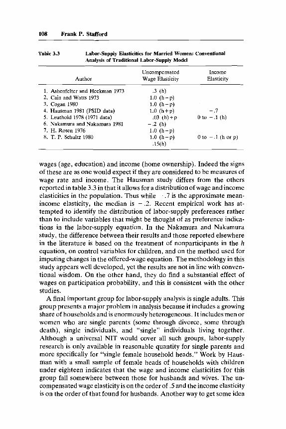
Table 3.3 Labor-Supply Elasticities for Married Women: Conventional Analysis of Traditional LaborSupply Model

Author Uncompensated Income Wage Elasticity Elasticity

1. Ashenfelter and Heckman 1973 2 . Cain and Watts 1973 3. Cogan 1980 4. Hausman 1981 (PSID data) 5. Leuthold 1978 (1971 data) 6 . Nakamura and Nakamura 1981 7. H. Rosen 1976 8. T. P. Schultz 1980

.3 (h) 1.0 (h+p) 1.0 (h+p) 1.0 (h+p) - .7 .03 (h)+p 0 to -.l (h)

- . 2 (h) 1.0 (h+p) 1.0 (h+p) 0 to - . l (h or p) .15(h)

wages (age, education) and income (home ownership). Indeed the signs of these are as one would expect if they are considered to be measures of wage rate and income. The Hausman study differs from the others reported in table 3.3 in that it allows for a distribution of wage and income elasticities in the population. Thus while - .7 is the approximate mean- income elasticity, the median is -.2. Recent empirical work has at- tempted to identify the distribution of labor-supply preferences rather than to include variables that might be thought of as preference indica- tions in the labor-supply equation. In the Nakamura and Nakamura study, the difference between their results and those reported elsewhere in the literature is based on the treatment of nonparticipants in the h equation, on control variables for children, and OR the method used for imputing changes in the offered-wage equation. The methodology in this study appears well developed, yet the results are not in line with conventional wisdom. On the other hand, they do find a substantial effect of wages on participation probability, and this is consistent with the other studies.

A final important group for labor-supply analysis is single adults. This group presents a major problem in analysis because it includes a growing share of households and is enormously heterogeneous. It includes men or women who are single parents (some through divorce, some through death), single individuals, and “single” individuals living together. Although a universal NIT would cover all such groups, labor-supply research is only available in reasonable quantity for single parents and more specifically for “single female household heads.” Work by Haus- man with a small sample of female heads of households with children under eighteen indicates that the wage and income elasticities for this group fall somewhere between those for husbands and wives. The uncompensated wage elasticity is on the order of .5 and the income elasticity is on the order of that found for husbands. Another way to get some idea


of the labor supply of female household heads is to look at the labor supply of married black women. Black families have historically had higher divorce rates than whites. Hence, a given married black woman is more likely to expect to be a single female household head.

If people formulate current labor-supply decisions in terms of their longer-run, expected marital status, and if current marital status is a less significant indicator of expected marital status for high-divorce-rate groups, evidence on the labor supply of black married women can be used for clues concerning the effect of “expected singleness” on labor supply. In this regard, Hausman’s estimates are consistent with Schultz’s results (see table 3.4). For virtually all age groups the total labor-supply elasticities for black married women are below those for white married women but above those for men (table 3.2). The results for nonmarrieds suggest that as more women (married or not) become “primary” earners or move along a continuum toward that end of the scale, they will have labor supply that is less responsive to the effects of income maintenance and tax systems.

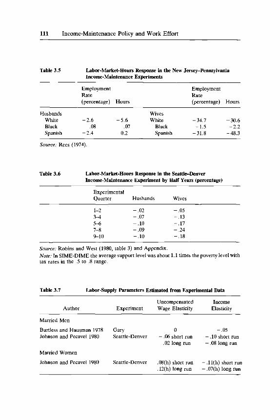
With our illustrative estimates of the traditional labor-supply model from conventional analysis, we now turn to a review of experimental analysis. Estimates from the three experiments are reviewed in tables 3.5 and 3.6. The major difference between the experimental method and the conventional method is not that the experiment is “theory free,” but that one hopes to obtain better exogenous variation in wage and income. As Rees argues, “in an experiment, differential tax rates create a truly exogenous source of differences in net wages” (Rees 1974). As the Hausman and Wise paper (chapter 5 ) demonstrates, there are serious practical problems that lead to voluntary participation and to selective attrition in the experiment. When this is so, a model of behavior, including both labor supply and participation in the experiment, is necessary. For purposes of this review, the assumption of random assignment will be made.

The results of the experiments, illustrated in tables 3.5 and 3.6, are consistent with the overall results from labor-market studies. In table 3.5 the major difference is between white and Spanish wives and all other groups. In table 3.6 the time response of labor supply is presented. Wives (two-thirds are white or Chicano) have a greater-percentage response to the treatment, and the temporal pattern is generally for a higher response the longer the duration of the treatment. This result is consistent with several of the hypotheses sketched out in section 3.1, including the leisure-on-sale model and the model of labor-supply choice subject to inertia from firm-specific work schedules and on-the-job training.

By using the experiments as a source of exogenous variation in wage rates and income, several authors have estimated labor-supply functions. These are illustrated in table 3.7. The results do not differ dramatically

Table 3.4 Elasticity Estimates of Labor Supply for Married Women

(1) (2) Participation Hours (3) Probability Worked Expected

(all persons) ( H 0) Labor Supply MLL OLS (1) + (2)

White Black White Black White Black Variable Wives Wives Wives Wives Wives Wives

Combined Labor Supply Model (all persons) (6)

Asymptotic t (4) (5) for (5)

OLS Tobit Tobit

White Black White Black White Black Wives Wives Wives Wives Wives Wives

Ages 14-24 Own wage Husband’s wage Nonemp. income

Own wage Husband’s wage Nonemp. income




Ages 25-34

Ages 3544

Ages 45-54

Ages 55-64

1.542 - .412

.0003

,860 - ,769 - .0062

.024

.047 - .0087

,034

,0150 - .195

1.57 - ,365 - .0084

,894

,0088 - ,964

1.58 - .288 - .0040

1.13 - 1.15 - ,0011

(5.88) (1.23) (.09)

(2.68) (1.76) (.40)

1.83 - ,382 - .001

1.12 - 1.06 - ,006

1.006 - 1.247

.0043

,861

,0028 - .932

,095

.0074 - ,463

,209 - ,334

.0025

1.10 - 1.71

.0117

1.07 - 1.27

,0053

,930

,0101 - 1.49

1.05 - 1.20 - .0003

1.16 - 1.65

.009

1.08 - 1.28

,002

(4.12) (6.40) (.80)

(5.53)

(.23) (3.98)

.I793 - .9704 - ,0207

.429

,0208 - ,673

- ,0448 - .383 - .0043

,201 - ,0579

.o005

,135 - 1.35 - ,0250

,630 - ,842 - ,017

.160 - 1.23 - ,0170

,598 - ,681

,020

,254 - 1.40 - .024

,590 - ,776

,022

(1.08) (7.08) (2.14)

(3.83) (3.11) (2.49)

.7529 - .9472 - .0553

.409 - ,848 - ,0117

.0719 - .282 - .0051

,271 ,0059

- .0056

,825 - 1.23 - ,060

,680 - .842 - ,017

,761 - 1.16 - ,0209

.714 - ,789 - .018

.946

- ,066 - 1.32

,647 - ,952 - .018

(4.74) (7.60) (3.98)

(3.58)

(1.33) (3.10)

1.690 - 1.223 - .0346

.681 - .747 - .0118

,284

.0065 - .I90

.115

.297 ,0022

1.97 - 1.41 - ,0281

,796 - .450 - .0096

1.93 - 1.34 - .023

,945 - .707 - ,017

,950 - ,919 - ,022

(7.09) (4.95) (1.60)

(2.37) (1.52) (.W

2.09 - 1.54 - ,050

Source: Schultz (1980)


Table 3.5 Labor-Market-Hours Response in the New Jersey-Pennsylvania Income-Maintenance Experiments

Employment Rate (percentage) Hours

Employment Rate (percentage) Hours

Husbands Wives White - 2.6 - 5.6 White - 34.7 -30.6 Black .08 .07 Black - 1.5 - 2.2 Spanish - 2.4 -0.2 Spanish -31.8 -48.3

Source: Rees ( 1974).

Table 3.6 Labor-Market-Hours Response in the Seattle-Denver Income-Maintenance Experiment by Half Years (percentage)

Experimental Quarter Husbands Wives

1-2 - .02 - .05 3 4 - .07 - .13 5-6 - .10 - .17 7-8 - .09 - .24 9-10 - .10 - .18

Source: Robins and West (1980, table 3) and Appendix. Note: In SIME-DIME the average support level was about 1.1 times the poverty level with tax rates in the .5 to .8 range.

Table 3.1 Labor-Supply Parameters Estimated from Experimental Data

Author Uncompensated Income

Experiment Wage Elasticity Elasticity

Married Men

Burtless and Hausman 1978 Gary 0 - .05 Johnson and Pecavel 1980 Seattle-Denver - .06 short run - .10 short run

- .08 long run .02 long run

Married Women

Johnson and Pecavel 1980 Seattle-Denver .08(h) short run - . l l ( h ) short run - .07(h) long run .12(h) long run


from those in most of the labor-market studies summarized in table 3.2, though there are what can be regarded as small differences in the reported results between Burtless and Hausman (1978) and others.

From the experimental- or labor-market-study estimates one can proceed to cost out a national NIT program in the short run. A brief summary of such estimates is given in table 3.8. The reason for negative cost entries under plan 1 is that it is less generous than the current system of transfer payments. The budget costs are highest for plan 2 since a larger guarantee and a lower tax rate lead the program to draw in many more families who would be eligible. Increasing the tax rate, which lowers the break-even income, lowers the costs dramatically.

In light of the small disparity between the experimental and nonexperimental results, a question that arises is whether the experiments were worth it. How does one go about answering such a question? The question is really one on the optimal scale of evaluation. Much of the literature on sample design for the NIT proceeds on the assumption of a known evaluation budget and then seeks to answer the question of whether the sample should be apportioned into various treatment groups based on the fact that the treatment groups have different costs per observation.

Table 3.8 Costs of NIT Based in SIME-DIME Results (1975)

Costs ($6 billion)

Number of Cost with

Plan Change (million) Supply Response Percentage Families No Labor Labor-Supply

1. G = 5 0 % , t = . 5 " Husbands - 7.0 Wives -23.3 Total H-W - 10.3 2.4 -0.1 0.2 Female Heads 0 2.3 - 1.9 - 3.0

2. G = loo%, t = .5" Husbands -6.2 Wives -22.7 Total H-W - 10.0 15.7 19.0 23.5 Female Heads - 12.0 3.6 4.0 4.5

3. G = 10070, t = .7" Husbands - 10.1 Wives - 32.0 Total H-W -20.6 5.8 6.5 9.6 Female Heads - 14.9 3.0 2.6 3.0

Source: Keeley et al. (1978). "Plans are defined by tax rate ( t ) ; percentage of poverty line represented by the guarantee (G).


Another way to proceed is to regard the experiment as part of a problem in statistical decision theory. A full elaboration of this approach is well beyond the scope of this paper, but it does seem worthwhile to outline the general idea. The first two ingredients in such an approach are: (1) listing the critical parameters about which we are uncertain and (2) relating these parameters to a loss function for policy-decision variables. In the case of NIT let us assume that there are two critical labor- supply parameters and two policy variables, G and t. How large a sample should be drawn given some known cost per sample point?

To answer this sort of question we must first begin by defining a function that relates gains to selection G and t , conditional on values of the unknown parameters. This can be set out with a labor-supply function and an indirect utility function for the NIT recipients as is done in Burtless and Hausman. The labor-supply function is given as

(1) h = k[w(l - t)]“(Y + G)b,

where h = hours of market work, w = wage, Y = nonlabor income, and a and b are the critical labor-supply parameters. Welfare of the recipients can be expressed as

k[w(l - t)]l+” (Y + G)’-b V = V[w(l- t ) , Y + GI = +- ,

l + a 1 - b

where v(.) is the indirect utility function or maximum utility that can be obtained given w(1 - t) and Y + G, for given values of a and b.

The “taxpaying” factors give a payment, P, of

(3) P = (G - twh)n

to the n recipient^.^ Substitution of equation (1) for equation (3) provides an expression for

the taxpayer costs. How does one translate this expression into a decision-theory framework to address the question of the optimal scale of evaluation? First, suppose we know a and b. What would be the optimal values of G and t? Here it seems necessary to impose an arbitrary social-welfare function. Following Orr (Orr 1976; Varian 1980, 19Sl), suppose the taxpayer gets Zutils from the utility of the welfare recipients.

(4) z = Z(V)

where 2’ > 0. One reason for this would be altruism. Another could be that the taxpayer assigns some probability that chance will place him or his heirs in the recipient category. If a and b are known, the task is to choose G and t to maximize taxpayers’ net utility.

4. This is obviously an oversimplification because who is a taxpayer and who is a recipient depends on whether G - twh is positive or negative for a given individual. Here we assume that all n recipients have known identical values of a and b.


(5) B = Z(V(w(1 - t ) , Y + G; a, b)) - P(G, t ; a, b) .

The reason for a social experiment or survey is to provide better information about a and b. These are not really known but are given by a joint prior probability density function (p.d.f.). Given the joint prior p.d.f., there can be defined an expected value maximizing choice of G and t in equation (5). Perhaps, however, we can do better through evaluation.

A sample that costs c per observation can be drawn to carry out the evaluation. As we contemplate samples of differing sizes, we may expect to leave the mean of the p.d.f. unchanged but to reduce the posterior variance. The incremental gain in the expected maximum value of B as we contemplate incremental sample sizes can be compared to the marginal sampling cost, c , ~ to determine an optimal sample size. In such an analysis the scale of the program (here, n ) will be important and could lead to a large evaluation expenditure of the magnitude involved for the NIT experiments.

Actual implementation of the approach set out in equations (1)-(5) would require a computer simulation and some prior-joint-density function for a and 6. Those skeptical of previous labor-market studies would want to use a diffuse prior, while Borjas and Heckman would want to use a rather tightly drawn prior. Simulation results would show a range of optimal sample sizes depending on the prior-density function. An important point of such an approach is that if the posterior mean values of a and b turn out to equal the prior means, this is not the basis for concluding that the experiments were not worth it. The expected postexperimental parameter precision will be greater and the expected value of the best policy can therefore be increased above its pre experimental value.

3.2.2 Unemployment Spells and Intermittent Labor-Market Attachment

Research on unemployment is based on two broad groups of theoretical models, which for the sake of discussion can be called rationing models or rational models. Rationing models postulate unemployment to be the consequence of events that limit a person’s ability to achieve a desired labor supply. The Keynesian involuntary-unemployment model is a rationing model. Constraints arising from lay-offs or reduced work hours lead to involuntary unemployment. In rational models people respond to exogenous events in a purposeful way. For example, the job-search models of unemployment regard informational investments as the source of time out of employment (Phelps 1970b), or in the models of Lucas and Rapping (1970) and Feldstein, (1978), in a downturn workers

5 . The cost per observation also depends on a and b but we can ignore it here.


take advantage of temporary discounts on leisure time and are not induced to work longer hours because the usual effects toward more market work when income falls are mitigated in an intertemporal setting.

Rather than develop a lengthy discussion of these theories, we will proceed by indicating some results from labor-market studies and the findings from research on SIME-DIME data.

The three labor-market studies we will discuss are those of Ehrenberg and Oaxaca (1976), Feldstein (1978), and Hamermesh (1980). These studies rely on what may be termed rational models. The Feldstein (1976) model postulates an implicit contract between the firm and its workers. The contract covers anticipated periods of high and low wages (based on high and low values of the firm’s output price) in light of knowledge of the unemployment insurance (UI) system. The UI system, by favorable income-tax treatment of benefits and imperfect experience rating of the tax for employer contributions to the UI system, encourages an implicit contract that places greater reliance on variations in the number of workers employed than on variations in hours per worker. Unemployed workers do not search but are only temporarily laid off in the sense that they anticipate eventual recall to their pre-lay-off job. The Ehrenberg and Oaxaca model postulates search behavior of the unemployed as motivated by a known dispersion of reemployment wages and knowledge of UI benefits. The Hamermesh model postulates maximization of the utility of expected income in light of a known value of the layoff probability, rules for UI benefits per week, and rules for potential duration of benefits.

Defining hours not on the job as reductions in labor supply, all three studies indicate possible labor-supply effects of the UI system. Ehrenberg and Oaxaca report that for older males who change employers, duration of spells of unemployment is increased by 1.5 weeks as a result of an increase in the replacement ratio from .4 to .5. Feldstein reports that for the mean replacement rate (3) about half of the temporary unemployment rate of 1.6 percentage points, or about 0.8 of a percentage point, is accounted for by UI benefits. The Hamermesh results also indicate that UI increases time not on the job for women by increasing the unemployment-spell duration. His work indicates that anticipated benefits also increase weeks worked per year. This suggests that the UI system creates incentives for intermittent labor supply on the part of women who would otherwise have a still weaker attachment to the labor force.

The labor-market studies are suggestive of the impacts one could expect from an NIT, but NIT benefits are not enhanced by previous labor-market earnings, and UI benefits are financed by experience-rated payroll taxes on employers, though some authors seem to believe it is so imperfectly experience-rated as to not be experience-rated at all. In the United States, UI benefits have been untaxed so annual earnings have


not affected benefits beyond their effect on eligibility. Because of substantial policy differences, a simple carry-over to NIT from labor-market studies on UI would be most tenuous. For these reasons the experimental results take on greater importance in evaluating a connection between unemployment and NIT.

A research memorandum by Robins and Tuma (1977) reports on treatment-control differences in the proportion employed and not employed, with an attempt to disaggregate those not employed into groups of “involuntarily unemployed” and “voluntarily unemployed.” The voluntarily-unemployed category may be termed “out of the labor force.” The results for wives (table 3.9) provide some interesting con- trasts with those of Hamermesh. Despite the large differences in theory and method between the two studies, it does seem that the NIT leads to reduced employment and increased unemployment at the expense of employment, whereas UI leads to an increase in both employment and unemployment at the expense of time out of the labor market.

3.2.3 Work Effort and Productivity

Both experimental methods and labor-market studies have treated respondent reports as the appropriate measure of labor supply, but it seems likely that work effort varies substantially across different jobs and that a person could respond to an income guarantee by reducing work effort rather than reducing elapsed hours on the job. As an empirical matter, work effort does vary substantially across types of jobs. For example, union members, particularly those in blue-collar operative jobs, report greater work effort (Duncan and Stafford 1980), partly because in capital-intensive production processes such as the assembly line, cost minimization by firms will lead to a faster work pace.

Suppose the rate of depreciation of the capital is, over some range, independent of the flow or rate of production per unit time. Then the rental rate for capital as a function of the production rate or work pace is a rectangular hyperbola with the hourly capital rental rate rising at a slower

Table 3.9 Observed Proportions in Employment States in SIME-DIME Control Treatment

Husbands Wives Female Heads ~~~

Employed .81 .78 .37 .31 .55 .52

Involuntarily unemployed .13 .16 .12 .14 .22 .22

Voluntarily unemployed .06 .05 .50 .54 .23 .26

Source: Robins and Tuma (1977, 28).


work pace and falling at a faster work pace. Consider a situation where workers have a U-shaped reservation wage function for work pace. Too slow a pace is boring and too fast a pace is fatiguing. Then cost minimization will lead to an outcome where workers are compensated to work at a pace beyond the minimum of their reservation wage function. The greater the capital-labor ratio, the further beyond the minimum will be the equilibrium work pace.

It is easy to imagine a slower work pace as a normal good. As income rises, the entire reservation wage function will shift upward and to the left, yielding a slower equilibrium work pace at a lower rate of capital utilization per unit time as well. Some empirical work by Scherer (1976) is consistent with this view, and causal reports of reduced work pace in U.S. auto assembly plants as income grew secularly are consistent with this sort of model. The income effects of the NIT should lead to a slower work pace or, more generally, reduced work effort.

A preliminary analysis of work pace and nonwork time on the job has been based on data from the Time Use Survey by the Survey Research Center of the University of Michigan (forthcoming). In addition to detailed time diaries, information was gathered on time spent in formal or scheduled breaks, in socializing, or in “personal business or just relaxing.” In an estimated equation to test some predictions of life-cycle training and labor-supply models, it was found that netting out training and nonwork time at work led to stronger age and education elasticities with effective work hours rather than elapsed hours on the job. As Harvey Rosen remarks, “To the extent that age and education are proxying for the wage, these results suggest that improper measurement of effective hours may be obscuring a positive wage response” (Rosen 1980, 173).

3.2.4 Training and Retirement

Do tax rates affect incentives to invest in human capital? In the well- known human-capital model of Ben-Porath (1967), this depends on whether the production of human capital requires both time and market inputs. When labor income is subject to a proportional income tax, the cost of investing is lowered along with the returns (Becker 1971). If the sole input to education is time, then both costs and returns are lowered by the same proportion. In the “neutral” case of the Ben-Porath model with no market inputs to human-capital production, the investment decision is unaltered by a proportional tax. In the simple model, leisure is not included in the objective function, so the question of income effects cannot be addressed.

If investment requires both time and market goods, a proportional income tax discourages investments since the price of only one input is reduced by a proportional income tax. As a result, investment declines. If


on-the-job training is regarded as using fewer market inputs, then we could expect a smaller training effect for adults than for those still in formal schooling.

In more complete models that include labor supply, clear results are difficult to obtain (Ghez and Becker 1975; Ryder, Stafford, and Stephan 1976; Blinder and Weiss 1976). This finding is of major importance in attempting to think of long-run incentive effects of NIT. Very difficult problems of theory combine with a paucity of long-term panel data from household surveys with exogenous tax-rate variations. The absence of good labor-market studies or experimental results leaves life-cycle training effects of taxes as true terra incognita, though Weiss, Hall, and Dong (1980) report a reduced training effect of NIT from the SIME-DIME study.

If one fears the unknown, one will not be comforted by the anomalous results in this literature which indicate that small changes in lifetime income and initial human capital can lead to a choice of radically different lifestyles: from one of little initial training with labor supply declining and leisure rising monotonically after an early life-cycle period, to one of large initial training with labor supply rising throughout most of the life cycle.6 The choice between these equal-utility life-styles could be training biased because one would receive all of the guarantee through the early life cycle when time is specialized to leisure and training.’ On the other hand, an NIT adds to the overall taxes on labor-market earnings and thereby would probably discourage training through substitution effects.

Research on the latter part of the life cycle has analyzed early retirement decisions with human capital exogenous. These studies imply that assets and Social Security “wealth” (discounted expected benefits) lead to early “retirement” (labor-market withdrawal or sharply reduced hours). Studies by Boskin (1972), Burkhauser and Turner (1978), and Quinn (1977), and research in progress by Tom Fraker (1981) clearly indicate impacts of Social Security wealth.

Fraker studies older unemployed male workers, using panel data to determine the resolution of unemployment spells. His question is whether, given health and other conditions prior to the unemployment spell, Social Security wealth induces a higher probability of “retiring” instead of becoming reemployed. The answer is clearly yes. For an older unemployed worker with a .5 probability of reentering the labor market, a one-standard-deviation increase in Social Security wealth would reduce the participation or reentry probability by .28.

6. Ryder, Stafford, and Stephan (1976,666). Recently several authors have emphasized aspects of income taxation that could encourage human-capital investments via insurance effects. See, for example, Eaton and Rosen (1980); Varian (1981).

7. This issue arises in the debate over college students being eligible for food stamps.


Based on these results for Social Security, is there anything that could be said about an NIT? One way to assess this is to consider the discounted NIT guarantee value as “NIT wealth.” This idea does not seem too far off, Even though the level of NIT wealth depends on a time path of labor supply, starting from any given possible “retirement” date, so too does Social Security wealth, at least over the age range of sixty-two to seventy- two. In this way it seems clear that a prediction of early retirement with an NIT is a warranted expectation. Moreover, Quinn’s results indicate a positive interaction of Social Security wealth and private pensions. In a similar fashion, if an NIT is available to increase retirement income or to tide one over until Social Security eligibility is obtained, this interaction could accentuate the increase in early retirements.

3.2.5 Divorce and Remarriage

One of the findings in the New Jersey-Pennsylvania and SIME-DIME analysis was that NIT treatments led to higher divorce rates (Bishop 1980). This finding can be regarded as a surprise in that, unlike the current public-assistance programs in many states, NIT payments are made to families regardless of whether or not the male adult is present. This result is less surprising in light of labor-market studies that show a strong effect of AFDC payments on the duration of spells of divorce.

One can develop a simple model of the sort implicit in Bishop’s discussion of marital instability. He talks of “independence effects” and “income effects.” To see these, suppose the husband ( M ) and wife ( F ) have separate utility functions, UM and U F . Within marriage there is defined a utility-possibility frontier that can be obtained by optimal variation in labor-market hours and nonmarket activity of both spouses in the absence of an income-support system. This is given in figure 3.1 as UPF.8 Outside of marriage there is some maximum utility attainable from becoming single (or finding another spouse), and this is given as URM for the husband and U R F for the wife.

Without the transfer system marriage continues, and the spouses may occasionally quarrel about where along the AB segment the family should be, The introduction of an income-support system should make the family better off (shifting the UPF outward to UPF’), but it can also increase well-being outside of marriage because some payment is available to single persons as well. Consequently, the U R M and U R F shift out from the origin to U R M ’ and U R F ‘ . As drawn in figure 3.1, the posttransfer

8. This sort of approach is adopted by Brown and Mauser (1977). See also Gerson (1981); Hill and Juster (1980). Rather than assume a common utility function, one can postulate family public goods as well as private goods for each partner entering into the individual utility functions. Empirical evidence indicates that time in household chores by one spouse substitutes for the other’s time in the household chores, but that spouses’ leisure-time activities are complementary.


“F

equilibrium would lead to dissolution. Here the independence effects dominate the gains within marriage effects.

To push the analysis a bit further, while the introduction of a cash transfer system can increase divorce rates when newly introduced, it may have a smaller long-run effect on divorce rates because marriages formed subsequent to its introduction will be based on new reservation utilities. It is changes in reservation utilities out of marriage rather than their level that affects divorce rates most strongly. This implies that the short-run effects of an NIT on divorce rates could be larger than the long-run effects.

AFDC payments conditioned on maintaining single status are another


matter. Analogous to UI, if AFDC is available contingent on maintaining a particular state (not married rather than not employed), then we would expect an effect on the duration of spells of divorce. Specifically, Hutch- ens estimates that if the AFDC guarantee of the high AFDC states (about $300 in 1971) were applied to the low AFDC states (about $60 in 1971), the two-year remarriage probability for a woman with three children would fall from S O to .15 (Hutchens 1979). This response seems to be very substantial.

A question would seem to be not whether NIT has an effect on remarriage but whether it has a smaller effect than a system it could replace, such as AFDC. In the NIT experiments one would expect that the remarriage rates conditional on divorce are affected less by the experimental treatment than by an AFDC-type system. If so, an NIT may affect duration of divorce spells, but less so than a system that has payments explicitly conditioned on marital status.

As we consider the areas of behavior, what have we learned from the experiments? To me it seems that, with the exception of areas productivity, training, and work effort, we have learned a substantial amount. Results based on the analysis of data collected in the experiment tell us there will likely be substantial behavioral responses to an income-support system. It would be unwarranted to conclude that a transfer-payment system can be designed without careful regard for work-incentive effects as well as other aspects of family decision making, including marital stability.

Avoiding unintended outcomes for national programs is extremely important. Better precision on various behavioral parameters is important because it can help us avoid such unintended outcomes. While a formal model of the optimal scale of evaluation for something as complex as an NIT is very difficult, my impression is that we have learned a great deal from the experiments. At a minimum, the experiments have reduced the variance of labor-supply parameters, even if they have not shifted the means very much. Such improvements in parameter precision are valu- able when applied to such an important social issue as income support. Further, the experiments represent a large social science data base that will help answer other important questions as more experience is gained in working with the data.

3.3 Directions for Future Research

Future research on labor supply, whether based on experimental variations in exogenous variables or on conventional household surveys, should focus on a number of shortcomings identified in section 3.2. These include pure measurement problems and problems with the theory. Neither of these areas received much attention within the experiments.


3.3.1 Some Methodological Problems

One of the universal labor-supply findings is that adult males have labor-supply responses that do not change much in light of wage and income changes. Although I do not think this finding is too far off, it could be quite wide of the mark on methodological grounds. Table 3.10 shows a comparison of hours per week from the time diary with hours per week based on respondent reports of usual hours on the job. In response to direct questioning, a remarkably high percentage of employed adult males claim to work forty hours per week and fall into the forty to forty-nine hours per week category. Generally, the off-diagonal entries to the southwest outnumber the off-diagonal entries to the northeast by about two to one.

One reason for believing that the time diary is a better basis for a point estimate of labor-market time is that the diary method is not directed to highlight a particular activity. Methodological work with beepers pro- grammed to emit a signal at random intervals led us to conclude that diaries provided unbiased estimates of most activities and that respondent reports usually overstate time in the specific activity.

Suppose that respondent reports of market work, particularly for men, are concentrated at forty hours per week when in fact the hours of market work have a lower mean and a greater variance. Then experimental or household surveys based on direct questioning will lead to a small apparent labor-supply response.

From our study we also estimated non-work time while at work in the market. Socializing, formal and informal breaks, and on-the-job training all reduce current labor supply. The disparity between respondent reports of work hours and diary hours adjusted for on-the-job training and leisure is very large. For men in the age groups under 25, 25-35, and 34-44, they are 40.1, 24.5; 42.8, 32.0; 41.1, 31.2, respectively (Stafford and Duncan 1980).

Table 3.10 Comparison of Alternative Hours at Work Measures for Employed Adult Males

Time Diary Report of Minutes Worked per Week Reported Hours per Week Under 1770- 2370- 2970 No Diary (average week) 1770 2369 2969 or more Time

Under 30 13 10 2 1 2 30-39 12 12 10 1 2 40-49 45 35 105 36 3 50 or more 6 10 23 27 0


3.3.2 Labor Supply through Time

Is there a connection between income-support systems and intermittant labor supply? Here we define intermittant labor supply as a temporal path of time at market work, with large variations including possible periods with no time at work and subsequent return. The traditional labor-supply model, particularly with progressive taxes, is virtually guaranteed to lead to a stable interior equilibrium provided wage rates and nonlabor income are unchanged. Intermittant labor-market activity is usually seen as the consequence of wage rates, that change through time because of business-cycle influences. The individual is postulated to take advantage of transient wage opportunities that arise through time from business-cycle or market specific wage changes. In such a setting various policies designed to stabilize income over the high- and low- demand periods can exacerbate cyclical swings in labor-market activity (Feldstein 1976).

A number of ways exist to explain intermittant labor supply in a world where wages do not vary through time because of changes in product demand. If the opportunity set is nonconvex and the utility function is subject to random fluctuations from period to period in the parameters that determine the relative value of leisure (e.g., simple shifts in the slopes of indifference curves), then rapid swings in desired work could appear from period to period even though the opportunity set is stable. An interpretation of such a model is that random events, such as a child’s illness or other nonmarket events, change the utility-function parameters from period to period.

The approach here is to develop a simple illustrative model that cap- tures the inherently variable nature of labor supply, at least for some sectors of the labor market, and then to ask what influence government policy could have on the path of labor-market effort, including periodic nonparticipation. Motivating factors for such a model include the secular rise in the unemployment rate and the evidence of intermittant labor- market behavior reported in section 3.2. The two critical elements that lead to periodic behavior in the model are scale economies in work effort as it relates to potential output (a type of nonconvexity) and a negative- feedback effect from sustained work effort to productivity potential. This type of specification squares with the observation that most labor markets are characterized by a wage premium for longer-duration employment spells and employment spells characterized by a larger fraction of time devoted to market activityeY Part-time jobs with short tenure usually pay

9. Note that measurement error in work hours will lend to a small apparent relation between average wage rates and hours, if wage rate is defined by dividing labor earnings by hours. Further, even if average hourly wage rises modestly for longer hours, the marginal wage can be rising sharply.


much lower wage rates to the same individual. The literature on firm- specific human capital highlights the incentives for firms to formulate work contracts that encourage employment over a longer duration, in order to realize returns on early investments. A second motivating fact is that most people actually work on an intermittant basis. They take weekends off. They take vacations. They have spells of non-participation in the labor market.“’ These occur in the absence of business cycles, though business cycles may certainly affect them. In the model set out below, such periods outside the labor market can regenerate market productivity.

A Model of Intermittent Work Effort and Unemployment

A decision to work leads to an output path that grows through time, but it also leads to a build-up of fatigue. The fatigue or reduced individual well-being acts to limit output and creates incentives to withdraw from work (or reduce work effort) to regenerate well-being. The disutility from work derives from work effort but also from fatigue. Just as in the traditional model, the gains from work include claims to output, but the model differs in that fatigue as well as work effort affect well-being. The disutility of work can be determined largely by cumulative effects of fatigue with a possibly small role for actual work effort.

The relationships between output, T, the well-being state, R, and work effort, u, are given by

(1) R = T ,

T T T = - C 2 R + g 1 U ,

where c 2 and g, are parameters with c2 > 0 and 0 < gl < 1, and I u I I 1. The individual well-being state is a supply-side factor. It can be thought

of as fatigue, and negative values imply that one is “fresh” and full of enthusiasm for work. Work output can be motivated on the demand side as well as on the supply side. On the demand side, firms have an interest in a sustained period of work effort, both because of job-specific training costs as well as other setup costs. On the supply side a worker can be more effective with a period of concentrated effort and attention at a given job. The intensity of work effort, u , can range from + 1 to - 1. The parameter, g,, can be thought of as a policy or productivity variable that affects the rate at which work effort is transformed into output available to the firm and its employees. It can include payroll taxes, personal income taxes, or any policy that alters the relation between work effort and output. A more complex specification could allow for a direct relation between u and R or a separate decision variable influencing R.

10. Another example is periodic urban migration from rural villages in less developed countries.


Consider a simple linear objective function where the flow of gains is defined as

(3)

In terms of an intertemporal objective function, we have a control problem of minimizing the negative of L over an infinite horizon. The intemporal objective function is

L = a n - R - y u .

(4) Jo = Jr - [UT - R - ' u ] dt ,

which is minimized subject to equations (1) and (2), and initial conditions on T and R.

To analyze this system it is convenient to transform the state variables R and n so that

C x1 =- R and

g1

We have the transformed-state equations as

(7)

The system (7) is known as the harmonic oscillator and is the basis for representing a wide variety of physical systems (Athans and Falb 1966). In this labor-supply model we will see that for our objective function, the model leads to an outcome of intermittant labor supply with piecewise continuous-control sequences of + 1, - 1, + 1, - 1, . . .

What is the control law for our system? If we define

(8) g2 = g1a 9

then our transformed system is

(9) min J1 = - [g2x2 - glxl - -yu]dt

plus equation (7) . The Hamiltonian for the transformed system is

(10) H = - g2x2 + g,x1 + y u + PlCXZ - P2cx, + P2U

= - g2x2 + g,x1 - P2cx1 + PlCXZ + u(P2 + y) *

Behavior of the System

Based on the general principle that

(11) H ( x * , u* , P * ) ( H ( X * , u , P * ) ,


for all admissable u and t E ( 0 , ~ ) (where * denotes values of the variables satisfying necessary conditions for an optimum), we can conclude that the optimal control is piecewise constant and is given as

(12) u* = - sgn (P2 + y)

where sgn denotes signum function." In analyzing this system we are interested in points where u* switches

from - 1 to + 1 and from + 1 to - 1. Given the system costate equations

(13) Pi = - 6 H / 6 ~ 1 = - g1 + c P ~ ,

(14) P2 = - 6H/8x2 = g, - cP , , and if P2 = 0 ,

then PI = g 2 / c .

We are interested in points where

(15)

and

and where

(16)

and

u* switches from + 1 to - 1 , P2(tl) = - Y

P2(tl> ' 0

u* switches from - 1 to + 1. P2(tl) = - Y

P2(tl) < 0

We know H = 0 (tf = and no specific time dependence in H ) (Athans and Falb 1966). If P2 = - y, then from (10) we have

- g2x2 + g,x, + u( - y + y) - ( - y)cx , + P1 cx2 = 0

or

From substituting equation (17) into equation (14) we have the following expression for P 2 :

11. n = sgn (m) means

n = + l i f m > O , n = - 1 i f r n < 0 , n undefined if m = 0

A possible difficulty is that the control law is not defined if P2 + y = 0 over some interval te ( t l , tz). If so, it can be shown that

P, = 0 = > P2 = g , / c > 0 .

This would contradictp, = - y, which implies that singular controls (where n is undefined) are not a concern here.


We can conclude then that

(19) i2>0 if xl,x2>0 or if xl,xz<O.

(20) P2<0 ifxl>O, x2<0 or ifx,<o, xZ>o .

The control law is defined by into which of the four quadrants the state variable pair falls. In quadrants I and 111, u* = - 1 and in quadrants I1 and IV, u* = + 1. The path of the state variables subject to a control sequence + (11), - 1 (I), + 1 (IV), - 1 (111) can be constructed by noting that if u = 0 through time, then (7) defines a circle with an origin of (0, 0). If u = + 1 through time, then the path is clockwise along a circle with an origin of (1, 0), and if u = - 1 through time, then the path is clockwise along a circle with an origin of ( - 1 , O ) . These trajectories are giveninfigure3.2. Apathsatisfyingequations(15), (16), (19), and(20) is given as a linking of segments of the various circles.

Discussion

An economic interpretation of the path suggests that there are two major phases-a work phase and what may be called a regeneration phase. Starting at A and moving clockwise the person begins from a period outside of the labor market with fatigue at its minimum. Entry into work is characterized by full effort (u* = + l), and combined with a low fatigue level, output rises rapidly until we reach B. From B on the person “coasts,” having built up a large productive capacity. One counterintui- tive result is that work effort slacks off (u* = - 1) when productivity is high. Does this make any sense? One way to consider it is to imagine an alternative plan, say, u = 0 or u > 0. In the case where u = 0 the path would be on a circle with the origin (0,O). This would lead to a future crossing of the x1 axis to the right of C and would hinder what can be termed the regeneration subarcs of CD and DA. In a sense u* = - 1 over BC forestalls an excessive build-up of fatigue. The regeneration phases consist of a segment of capital rebuilding and leisure (CD and DA). On the CD segment, u* = + 1 is required to build up productivity for a future work period given fatigue effects. On the DA segment, u* = - 1; this can be viewed as prework recreation which will lead to a more productive work period.I2

Before turning to effects of changes in the parameters c andgl, it can be

12. One colleague has remarked that the full path reminds him of the academic year with DA late summer, AB fall semester, BC winter semester, and CD early summer.

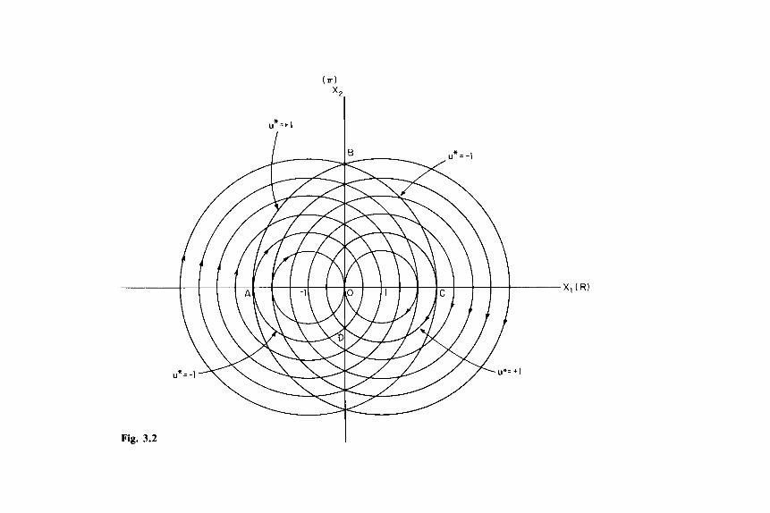
x


remarked that part of the BC segment could be thought to correspond to income support contingent on recent labor-market history. A large number of proposals have been advanced to make income transfers available only for those “willing to work.” If this translates into recent work history as a condition for income support (as with UI), then the BC segment could consist of drawing down on income eligibility. In part, an eligibility for future benefits can be thought of as defining our state equation which has an inherent scale economy in that .ir = f(u), rather than 7~ = f(u). This has been discussed in several recent models of labor-market behavior. l 3

What are the effects of reducing g, on labor-market behavior? A lower value can be thought of as an increased tax. Consider initial values ofg, = c = 1. In this case the transformed system (7) is coincident with the original system (1) and ( 2 ) . If g, is reduced, the absolute value of R and T

are reduced by that proportion in figure 3.2 . This implies that with a “tax” on work effort, the work phase is characterized by smaller positive output. The time required to move along an arc in figure 3.2 is given by the angle defined by the two line segments connecting the origin of the circle to the endpoints of the arc. What this implies is that time in the labor market is not influenced, though output from the path through the positive half-plane is reduced.

Effects of changes in other parameters on the solution are less readily interpretable as policy measures. A reduction in c2 leads to a path that moves through the x1x2 plane at a slower rate. If one thinks of adult workers as better conditioned to cope with fatigue effects of work, we would expect longer duration work spells in comparison with teenagers, who are less socialized to the world of work.

The point of our model is to indicate that a theory specifically oriented to represent intermittant labor supply can be developed. Research along these lines seems an important complement to the rapid growth of econometric studies on panel data and evidence from the NIT experiment on hours of work through time. These empirical results indicate that a great deal of labor-market activity is intermittant, a finding that takes on importance if the introduction of income-support systems leads to not only reduced average work hours but to a greater number of switches between market and nonmarket states. Moreover, our model suggests that while the time on the job and the frequency of switch may not change, the output can be reduced via taxes.

One puzzle in the model is that parameters in the objective function do not appear to alter the system behavior. My belief is that the simplicity (linearity) of the objective function reduces the system dependence on

13. Concerning UI effects see Mortenson (1977). Burkhauser and Turner (1978) have employed a model where Social Security leads to a connection between current work and future-income eligibility. This model leads to greater work effort in the prebenefit period.


these parameters. However, the potential for a model of this sort is not restricted to the linear objective function or the linearity in (1) and (2). In fact, as long as u enters equation (2) linearly, and F(T) and G(R) in R = F(T) and .ir = - G(R) are increasingly weak concave functions, a much more general objective function will still lead to solutions characterized by closed orbits.

3.3.3 Taxes, Television, and Work Effort

Based on current knowledge of labor supply, the issue of whether an NIT plan will ever be adopted can be raised. My guess is that a consensus still exists among economists that a modest scale NIT is a good public policy. Perhaps it does not appear as straightforward a matter as when Tobin and Friedman proposed it some fifteen or twenty years ago, but the idea does not look that bad either.

Although Congress has voted down NIT proposals with remarkable regularity, there has been an evolutionary series of changes in the federal food stamp program which have gradually moved it from a program to help with the distribution of “surplus” food to something close to an NIT. The change adopted in January 1979, which eliminated the purchase req~irement,’~ reduced substantially the voucher aspects of the program. As a consequence we have something close to an NIT in the current federal food stamp program. Did research have anything to do with this change? I think so, since many of the policy analysts concerned with the program felt that a move toward an NIT program was desirable.”

Has the evolutionary adoption of an NIT-like food stamp program reduced work incentives? I believe that it has had some effects based on the empirical evidence reported above and the fact that longer-term responses to wage and income effects are expected to exceed short-run effects. Further, the measurement of hours and the calculation of wage rates by dividing earnings by the same hours measure is likely to lead to an underestimate of the labor-supply response to wage rates. This tendency for errors in variables to convert what would be a positive labor-supply function to a negative one has been termed “division bias,” and recent evidence suggests it could be substantial (Borjas 1980).16 If in fact labor-supply functions are positively inclined for men, then the wage

14. Here is an illustration of the system before 1979. If a family eligible for $100 a month of food stamps at zero income had a monthly income of $200, then they had to pay $60 cash as the purchase requirement (with a benefit reduction rate of .3) to receive the $100 of food stamps. Although the “bonus value” of the stamps was only $40 ($100 less $a), barring illegal resale of the stamps, they had to spend at least $100 on food if they participated in the program. Now such a family would simply receive $0 worth of food stamps.

15. Research shows that the pre-1979 program did have voucher-like impacts. The marginal propensity to consume food out of food-stamp benefits was much higher than for other income sources. See Benus, Kmenta, and Shapiro (1976).

16. This has occurred to a minor extent with home repairs being the only market or nonmarket work activity to experience an increase between 1965 and 1975.


effects of an increase in the tax rate t would lead to reduced work, as would the guarantee. The benefit-reduction rate in the Food Stamp Program of about .3 can be regarded as a tax on labor income.

Another phenomenon is the secular rise in “full-employment rates” of unemployment in the United States. My view is that some specific theoretical work, perhaps along the lines suggested in this section, would lead to some empirically testable implications. Out of this we may gain a better understanding of the links between types of income-support systems and intermittent labor supply, including unemployment. In any event, it would seem desirable to explore a wider range of possible labor-supply models.

One of the findings from our time-use survey appears to lie outside the realm of accepted wisdom. Data comparing time use of those in the labor market between 1965 and 1975 show a rather strong shift away from work time, both in the market and at home, toward passive activities such as personal care and TV viewing. This shift can be seen in table 3.11. Part of this finding may be a cohort effect, since the 1975 cohort of 19 to 24 years old has a far smaller amount of total labor-market time (328 minutes per day) in comparison to the 1965 cohort of 19 to 24 year olds (408 minutes per day). However, the 25 to 34 and 35 to 44 year olds of 1965 who are 1975’s 35 to 44 and 45 to 54 year olds respectively, exhibited declines in total market work time of 415 to 387 minutes per day and 409 to 373 minutes per day. Further, the 45 to 54 year olds of 1965, who worked 397 minutes per day in the labor market, were working 323 minutes per day as the 55 to 64 year olds of 1975. Hence, the decline in labor-market time appears to hold across all age cohorts rather than simply being less hours worked by fresh cohorts of young people.

Other notable changes in time use between 1965 and 1975 include the very dramatic rise in time spent viewing TV by the college-educated, higher-income, professional and female respondents and a large percentage rise in active leisure and household repairs such as maintenance and gardening. However, the groups with the largest increases in active leisure and household repairs are quite different. For the former those with the largest increases are in the lowest-income groups, and for the latter the largest increases are for managers, professionals, craftsmen, and operatives.

The overall shift toward passive activities is not consistent with a rising wage rate, since many such activities are very time intensive, and rising taxes on market earnings should lead to a shift toward nonmarket work. One can employ a household-production approach to gain some insight on the matter. The widespread availability of color TV and the attempt of the networks to capture a better-educated and higher-income audience can be regarded as a home-technology shift that has favored this activity and led to more time in passive activity. What this suggests is that the

Table 3.11 Time Use of Men and Women by Minutes per Day at Work and at Home, 1965 and 1975

Labor-Market Time" Work at Home

House- hold Shop-

Travel Repairs, ping, Total Main Second to House- Upkeep, Child Finan- Work

Totalb Job Job Work work Gardening Care cia1 Time

1965 1975 1965 1975 1965 1975 1965 1975 1965 1975 1965 1975 1965 1975 1965 1975 1965 1975

Average 409 367 350 318 7 3 37 33 76 64 8 13 19 19 47 40 559 500 Married men 451 428 383 365 9 7 43 40 23 25 13 18 17 15 44 37 548 523 Unmarried men 454 353 394 309 8 2 33 34 37 38 2 10 5 5 36 29 534 435 Married women 337 276 294 242 2 0 28 21 181 143 4 10 29 31 51 55 602 515 Unmarried women 350 353 300 305 5 0 31 32 121 89 2 7 19 27 56 41 548 517

Passive Leisure Total

Per- Orga- TV Other Non- sonal Educa- niza- Social Active View- Activ- work Sample Care tion tions Events Leisure ing ities Time Size'

1965 1975 1965 1975 1965 1975 1965 1975 1965 1975 1965 1975 1965 1975 1965 1975 1965 1975

Average 647 662 11 20 16 15 39 34 24 34 84 117 60 55 881 937 864 557 Married men 639 642 10 18 16 15 35 29 26 31 103 132 62 51 891 918 448 248 Unmarried men 636 667 20 34 15 12 78 48 27 59 73 118 57 66 904 1004 73 88 Married women 652 685 4 7 9 16 30 35 23 24 59 105 62 53 839 925 190 119 Unmarried women 671 684 17 20 23 10 46 36 18 24 68 94 54 55 893 923 152 104

Source: National time-use surveys conducted by the Survey Research Center of the University of Michigan. "Labor-market participants was defined by ten or more hours of work per week. bIncluding time at lunch. 'Subgroup sample sizes may not add to totals due to missing data.


Table 3.12 Estimates of Weekly Hours at Work by Sex and Marital Status, 1965-76

Time Diary Estimates for Those Working"

Normal Work Travel to Work

Percent 1965 1975 Change

Percent 1965 1975 Change

Married men 44.7 41.3 - 7.6 Unmarried men 46.0 35.2 -23.5 All men 44.9 39.9 -11.1

Married women 34.3 26.5 -22.7 Unmarried women 34.9 35.6 +2.0 All women 34.6 30.8 -11.0

5.0 4.5 -10.0 3.9 4.4 +12.8 4.8 4.2 -12.5

3.2 2.3 - 28.1 3.6 3.7 +2.8 3.4 2.9 -14.7

Current Population Survey Estimates

Hours Worked Last Week Participation Rates

Percent Percent 1965 1975 Change 1965 1975 Change

Married menb 44.2' 42.9' -2.9 95.5' 92.2d -3.5 Married womenb 34.5' 34.0' -1.4 38.7' 49.0d 25.6 Men, 20-64 years 43.9 42.6 -3.0 94.6' 92.2" -2.5 Women, 2 M 4 years 35.7 35.0 -2.0 51.7" 58.5' 13.2

Source: See table 3.11. "Hours of normal work were defined to include regular work for pay outside the home or brought home, overtime, waiting or interruption during work time (for example, machine breakdown), and coffee breaks. Data are weighted using day of the week as a stratification variable and are available only for those reporting at least ten hours per week in the labor market. bMarried, spouse present. dMay. 'November 'April.

United States has been moving toward what my colleague, John Robin- son, has referred to as the "post-industrious'' society, with large shifts toward passive forms of leisure for reasons in addition to taxes and income-support effects. If so, this shift could be a major source of the apparent productivity decline of the last decade. What our data seem to indicate is that, as a first approximation, we are simply working less, as well as possibly working less productively. While our time-diary data show substantial declines in work hours, official statistics do not (see table 3.12), and in fact, this disparity can account for much of the recorded productivity decline (Stafford and Duncan 1980).

One more view of labor supply is that "leisure activities" and market activities are complements. The industrial revolution gave rise to interest


in “hobbies” which mirror innovation and thought at work. Our time- diary data are consistent with this leisure-and-work-as-complements hypothesis. For example, craftsmen and operatives are most likely to seek out physically active recreation. Of course, it is possible that certain types of work sort out people with certain inclinations and preferences, but it is possible that leisure and work reinforce each other. If so, should we consider reverse ca~sa t ion?’~ That is, will a major exogenous shift to passive activities outside the workplace lead to mental capital that is less productive in the market? Perhaps. If so, we may need a labor supply- side economics to explain the decline in productivity growth and hours of market work by a more inclusive group than the working poor. A model of the type in section 3.3.2 could be used to represent the connection between leisure-time activity and the regeneration of market productivity.

Comment Sherwin Rosen

Frank Stafford’s paper is a thoughtful and wide-ranging review of income-maintenance experiments and labor supply. He begins by discus- sing the relationship between experiments and economic theory and concludes that experiments cannot be agnostic about matters of theory: there is an intimate connection between the two. Theories discipline thought on what questions to ask and how to ask them, and thinking of data in the context of an econometric model adds precision to the analysis and interpretation of results. But that is true whether the data come from social experiments or from “market experiments.” The main virtues of social experimentation are to obtain more useful information on a particular question than is contained in available data (often collected for some other purpose) on market outcomes and to acquire superior control over variation in those exogenous variables thought to influence behavior. The better the data and experimental design, the less elaborate the model and analysis needed to answer the interesting questions. A test of any hypothesis is simultaneously a joint test of all the maintained hypotheses necessary to interpret it, and there is no way of separating the two, given the data. The less maintained the hypotheses, the better. Good experimental design can minimize potentially important interven- ing factors.

This line of thought suggests a trade-off between elaborate designs and

17. Sociologists have argued for a connection between work and leisure life-styles.

Sherwin Rosen is professor of economics, University of Chicago, and research associate, National Bureau of Economic Research.


elaborate models. Consequently, the optimum experiment will combine theorizing and design in the most economical proportions. The tighter the design around some very specific theory, the more likely are things of importance to be left out. All good theories are gross simplifications of actual behavior, and blind adherence to a specific theory can lead one wildly astray, unless of course the theory happens to be the correct theory. The costs of social experiments are sufficiently great that the prudent course includes some hedging. The design must be flexible enough to incorporate a wide class of influences and behavioral responses, yet not so wide that it cannot discriminate among alternative models.

The economic content of income-maintenance experiments has been greatly influenced by the neoclassical analysis of labor supply originating in the work of Paul Douglas and Lionel Robbins-the prevailing economic view on these matters in the 1960s when the possibility for experiments came to be realized. It is clear in retrospect that the simple neoclassical theory is a special case of a more general theory of time allocation, one in which Stafford’s own work with time-budget data will play an important role toward further development and refinement. The neoclassical theory is fundamental, but there is a host of broader and more complex issues that must be considered. First, the marked increase in marital instability in the 1970s raised important questions about the nature of the income-support unit. Is the support unit the individual or the family, and how should the family be defined for these purposes? Whose welfare is it that we wish to change by these subsidies, and how do subsidies interact with private transfer mechanisms within and between families? Second, the nature of the choice set facing potential workers has been clarified in recent years. The many dimensions of labor supply include weeks worked, hours per day, full-time or part-time, etc., and supply responses to subsidies may differ among them. Furthermore, the nature of many employment contracts may dictate different restrictions on hours variation on a given job than between jobs, so a person’s choice of labor supply may be a simultaneous choice of an employer offering the desired wage-hours package. Jobs are heterogeneous in many other dimensions. Stafford’s work indicates that there is considerable variety and trend in what can be termed “on-the-job” leisure, or the intensity of work. There are a host of other factors as well, including general working conditions, opportunities for advancement, skill acquisition, and the like. How do income-maintenance schemes influence these other dimensions of choice, and how do these forces interact in determining the final distribution of welfare in society? If a given scheme was actually adopted, how would the organization of labor markets be altered to respond to the changing needs and desires of workers that are affected? The emergence of panel data (of which, perhaps, negative-income-tax experimental data


are no small part) has widened the scope of labor-supply inquiry to incorporate life-cycle considerations. To what extent do we want income maintenance to subsidize transitory deviations from permanent, life- cycle earnings relative to life-cycle earnings themselves? What deter- mines the length of working life and retirement decisions? What roles do intermittent labor-force attachment and unemployment spells play in this, and how do income-maintenance subsidies and other social- insurance programs affect this class of behavior? We have come to recognize that there are important interpersonal differences in preferences and opportunities that are known to economic agents but which cannot be observed by investigators. These differences lead to compli- cated selectivity issues which interact with observed behavior and which must be treated statistically by maintained assumptions on distributions of unobservables. Estimates are known to be sensitive to assumed-func- tional forms, which cannot be verified.

These important points, some of which and more are discussed at length in Stafford’s paper, apply independent of how actual-behavior data are generated. They are as valid for social experiments as for market experiments. It is a truism that so long as there is scientific progress, something of interest will be left out of any investigation. I take it as an indication of the fruitfulness of applied economics in this particular area that so many new developments have come forward in recent years and that perhaps the rate of obsolescence is higher than in other areas. The larger it is, so much the better! There is no denying that many of these factors, including the work on marital instability, variable length of horizon among experimental subjects, and localizing the experiment in a single market area, have been at least partically anticipated in the experimental design; these issues are difficult to handle in market experimental data. No doubt there is room for improvement. There is also greater hope for handling selectivity issues with experimental data. Ran- dom assignment of experimental subjects to a wide variety of treatments can overcome many thorny selection problems that simply cannot be handled except by excessively complex statistical models in nonexperimental data.

What are we to make of the fact that experimental results have been more or less similar to findings from nonexperimental data? First, the comparison is not entirely complete because most nonexperimental results have been derived from the same or very similar sets of data. Also, it is well known that estimated income effects from nonexperimental data for males typically yield unsatisfactory results, often suggesting on face value that leisure is an inferior good. And since sharp estimates of income effects are crucial in going from uncompensated to compensated behavior, which in turn is necessary for welfare analysis, the potential for improvement with experimental data is apparent. Second, that the results


would be similar could not have been known in advance. Many of the nonexperimental results were arrived at first; perhaps analysts of experimental data have followed the privately optimal research stopping rule of ceasing analysis when an acceptable result was found. Perhaps further analysis going beyond existing results will change the conclusions. Third, that theories become obsolete with new findings surely does decrease the discounted future benefits of any analysis, but again that is true of both experiments and nonexperiments. If it is possible to handle some of these new factors in nonexperimental data, then the methods and extensions of maintained hypotheses that are necessary to do so can be just as well applied to experimental data too, and with more informative sources of variation added in the bargain.

It has been said that one of the main things economists have learned from social experiments is how to run experiments. To my mind that is surely a second-rate benefit because it is an awfully expensive way to learn. A superior way of learning some of the methods is to become involved in survey research at the grass-roots level. So far we as a profession have engaged in excessive division of labor with regard to microdata collection. Thinking about survey instruments themselves and how they relate to economic phenomena and economic theories is probably an area where the social rate of return is fairly large. The apparent divergence between relative private and social rates in this use of economists’ time, compared to other uses, is a fact worth contemplating.

Comment Zvi Griliches

At least three topics are covered in Stafford’s excellent paper: (1) Do we need social experiments? (2) What do we know about what an NIT would do and how (where from) do we know it? and (3), the importance of “effort” and the implication of the changing uses of time on the measurement of “real” hours of work. I shall comment only on the first two.

The tone of the paper appears to question the utility of social experiments. As I see it, we need experiments for two related reasons: (1) randomization of treatment allows us to ignore a whole slew of otherwise complicating variables and considerations; (2) application of treatment makes the relevant variable “exogenous.” In observational field-survey studies we are never sure how a particular X arose and whether or not the causality runs the other way, from the variables we treat as dependent to X .

Zvi Griliches is professor of economics, Harvard University, and research associate, National Bureau of Economic Research.


Surveys are also subject to the problem that little relevant information is found in the observed variation in Xit , either over people or over time. Consider, for example, housing prices or wage rates. In cross sections, the variation is largely due to quality differences. Over time, the “real” variation is largely common to all individuals or areas and is confounded with other time-series events, while purely individual variation is largely transitory or erroneous. Here is where experiments can and do help. They, in turn, are subject to serious self-selection and attrition problems, but so also are survey panel data. Good experimental design could alleviate such problems significantly.

The tone of the paper indicates that the view that experiments help is “simplistic.” Is it really? Experiments turn out to be difficult, compli- cated, and often botched up. I am not ready to say that good, simple experiments could not be run. Most of the earlier ones were too ambi- tious. (Reminds me of my view about econometric research, which parallels the Downs Law of Traffic Congestion: as new data sources become available, models and the questions they ask expand to the point that average certainty [validity] of the answers remains the same-all t-ratios tend to 2.) Stafford argues that because we will want to extrapo- late, we will want to fit a structural model after all, and for that we will need a wider range of variation (such as contained in surveys). I agree with Hausman and Wise that it is better to know something right in a small range, than be quite uncertain about what the wider-range relationship may actually mean. I am less worried about the extrapolation problem (similar problems arise, after all, in the analysis of survey data). I do not disagree, however, with Stafford that ultimately we want a structural theory, and hence we have to either fit it to or integrate it with the experimental results. The role of theory is threefold here: it should be guiding the experiment; it may be changed by it; and it could be changing exogenously, thereby making the experiment less interesting than was thought originally.

Ultimately Stafford concludes that theory and survey data complement experiments and help in their interpretation. I have no quarrel with that conclusion except to note that we would be less secure in our interpretation of the survey-based results if the experimental ones had not come out in the same ball park.

References

Abowd, John, and Orley Ashenfelter. 1978. Unemployment and com- pensating wage differentials. Paper presented at the NBER Universi- ties Conference on Low Income Labor Markets.


Ashenfelter, Orley, and James Heckman. 1973. Estimating labor supply functions. In Zncome maintenance and labor supply. See Cain and Watts 1973.

Athans, Michael, and Peter L. Falb. 1966. Optimal control: An introduction to the theory and its applications. New York: McGraw-Hill.

Becker, Gary S. 1971. Economics of discrimination. 2d ed. Chicago: University of Chicago Press.

Ben-Porath, Yoram. 1967. The production of human capital and the life cycle of earnings. Journal of Political Economy 75 (August): 352-65.

Benus, Jacob, Jan Kmenta, and Harold Shapiro. 1976. The dynamics of household budget allocation to food expenditures. Review of Eco- nomics and Statistics (May): 129-38.

Bishop, John. 1980. Jobs, cash transfers, and marital instability: A review and synthesis of the evidence. Journal of Human Resources 15 (Sum- mer): 301-34.

Blinder, Alan, and Yoram Weiss. 1976. Human capital and labor supply: A synthesis. Journal of Political Economy 84 (June): 449-72.

Borjas, George. 1980. The relationship between wages and weekly hours of work: the role of division bias. Journal of Human Resources 15 (Summer): 409-23.

Borjas, George, and James Heckman. 1979. Labor supply estimates for public policy evaluation. In Proceedings of the thirty-jirst annual meeting. Chicago: Industrial Relations Research Association.

Boskin, Michael. 1977. Social security and retirement decisions. Eco- nomic Inquiry 15 (January): 1-25.

. 1967. The negative income tax and the supply of work effort. National Tax Journal 20: 353-67.

Brown, Murray, and Marylin Mauser. 1977. Bargaining analysis of household decisions. Paper presented at the Conference on Women in the Labor Market, Barnard College.

Burkhauser, Richard, and John Turner. 1978. A time series analysis on social security and its effect on the market wage of men at younger ages. Journal of Political Economy 86 (August): 701-15.

Burtless, Gary, and Jerry A. Hausman. 1978. The effect of taxation on labor supply: Evaluating the Gary Negative Income Tax Experiment. Journal of Political Economy 86 (no. 6): 1103-30.

Cain, Glen G., and Harold W. Watts, eds. 1973. Zncome maintenance and labor supply. New York: Academic Press.

Cogan, John. 1980. Married women labor supply: A comparison of alternative estimation procedures. In Female labor supply: Theory and estimation, ed. James Smith. Princeton: Princeton University Press.

Deardorff, Alan, and Frank Stafford. 1976. Compensation of coop- erating factions. Econornetrica 44 (July): 671-84.


Duncan, Greg J., and James Morgan, eds. 1977. Five thousand American families: Patterns of economic progress. Ann Arbor: Survey Research Center, University of Michigan.

Duncan, Gregg J., and Frank Stafford. 1980. Do union members receive compensation wage differentials? American Economic Review 70 (June): 355-71.

Eaton, Johnathan, and Harvey Rosen. 1980. Taxation, human capital, and uncertainty. American Economic Review 70 (September):

Ehrenberg, Ronald G., and Ronald Oaxaca. 1976. Unemployment insurance, duration of unemployment, and subsequent wage gain. Amer- ican Economic Review (December): 754-66.

Feldstein, Martin S. 1978. The effect of unemployment insurance on temporary layoff unemployment. American Economic Review (December): 834-46.

.1976. Temporary layoffs in the theory of unemployment. Journal of Political Economy 84 (October): 937-57.

Fleisher, Belton, Donald Parsons, and R. D. Porter. 1973. Asset adjust- ment and labor supply of older workers. In Zncome maintenance and labor supply, 279-327. See Cain and Watts 1973.

Fraker, Thomas. 1981. The effects of social security wealth for the resolution of unemployment spells of older men. Ph.D. diss., Univer- sity of Michigan.

Friedman, Milton. 1962. Capitalism and freedom. Chicago: University of Chicago Press.

Gerson, Janet. 1981. The allocation of time in the household: A theory of marriage and divorce. Ph.D. diss., University of Michigan.

Ghez, Gilbert, and Gary Becker. 1975. The allocation of time and goods over the life cycle. National Bureau of Economic Research. New York: Columbia University Press.

Greenberg, David H., and Marvin Kosters. 1973. Income guarantees and the working poor: The effect of income maintenance programs on the hours of work of male family heads. In Income maintenance and labor supply, 14-101. See Cain and Watts 1973.

Hall, Robert E. 1973. Wages, income, and hours of work in the U.S. labor force. In Income maintenance and laborsupply, 102-62. See Cain and Watts 1973.

Ham, John. 1977. Rationing and the supply of labor: An econometric approach. Working paper no. 13. Industrial Relations section, Prince- ton University.

Hamermesh, Daniel F. 1980. Unemployment insurance and labor supply. International Economic Review (October): 517-27.

Hausman, Jerry A. 1981. Labor supply. In How taxes affect economic

705-15.


behavior, ed. Henry Aaron and Joe Pechman, 27-72. Washington, D.C., Brookings Institution.

Heckman, James. 1977. New evidence on the dynamics of female labor supply. Paper presented at the ASPER-DOL Conference on Women in the Labor Market, held in New York.

Hill, Martha S. , and F. Thomas Juster. 1980. Constraints and com- plementarities in time use. Survey Research Center, University of Michigan.

Hotz, Joseph. 1978. Discussion. In Proceedings of the thirty-first annual meeting. Chicago: Industrial Relations Research Association.

Hutchens, Robert M. 1979. Welfare, remarriage, and marital status. American Economic Review 69 (June): 369-79.

Johnson, T. R., and J. H. Pencavel. 1980. Utility-based hours of work functions for husbands, wives, and single females estimated from Seattle-Denver experimental data. Research memorandum 71, Stanford Research Institute, Menlo Park, Calif.

Kalacheck, E. D., and S. Q. Raines. 1970. Labor supply of lower income workers. In Technical Studies, President’s Commission on Income Maintenance Programs, 159-86. Washington, D.C. : GPO.

Keeley, Michael C., Philip K . Robins, Richard W. West, and Robert G. Spiegelman. 1978. The estimation of labor models using experimental data. American Economic Review (December): 873-87.

Leuthold, Jane H. 1978. The effect of taxation on the hours worked by married women. Industrial and Labor Relations Review 31 : 520-26.

Lillard, Lee A. 1978. Estimation of permanent and transistory response functions in panel data: A dynamic labor supply model. Annales de I’ZNSEE 30 (no. 1): 367-94.

Lucas, Robert, and Leonard Rapping. 1970. Real wages, employment, and inflation. In The microeconomic foundations of inflation and unemployment. See Phelps 1970a.

Masters, Stanley, and Irwin Garfinkel. 1977. Estimating the labor supply effects of income maintenance experiments. New York: Academic Press.

Metcalf, Charles. 1973. Making inferences from controlled income maintenance experiments. American Economic Review 63 (June): 478-83.

Mortenson, Dale. 1977. Unemployment insurance and job search decisions. Industrial and Labor Relations Review 30 (July): 505-17.

. 1970. Job search, the duration of employment and the Phillips curve, American Economic Review 60 (December): 847-62.

Munts, Raymond. 1970. Partial benefit schedules in unemployment insurance: Their effect on work incentive. Journal of Human Resources 5 (Spring): 160-76.


Nakamura, Alice, and Masao Nakamura. 1981. A comparison of the labor force behavior of married women in the United States and Canada, with special attention to the impact of income taxes. Econ- ometrica 49 (March): 451-90.

Orr, Larry. 1976. Income transfers as a public good: An application to AFDC. American Economic Review 76 (June): 359-71.

Phelps, Edmund S. , ed. 1970a. The microeconomic foundations of inflation and unemployment. New York: W. W. Norton.

. 1970b. Introduction: The new microeconomics in employment and inflation theory. In The microeconomic foundations of inflation and unemployment. See Phelps 1970a.

Quinn, Joseph. 1977. Microeconomic determinants of early retirement; A cross-sectional view of white married men. Journal of Human Re- sources 12: 329-46.

Rees, A. 1974. Summary of results on negative income tax. Journal of Human Resources 9 (Spring): 158-80.

Robins, Philip K., and Nancy B. Tuma. 1977. Changes in rates of entering and leaving employment under a negative income tax program: Evidence from the Seattle and Denver Income Maintenance Experiments. Research memorandum 48, Stanford Research Insti- tute, Menlo Park, Calif.

Robins, Philip K., and Richard W. West. 1980. Program participation and labor supply response. Journal of Human Resources (Fall): 524-44.

Robinson, John P. 1980. Alternative methods of measuring time use. Survey Research Center, University of Michigan.

Rosen, Sherwin, and Finis Welch. 1971. Labor supply and income redis- tribution. Review of Economics and Statistics 53: 278-82.

Rosen, Harvey. 1980. What is labor supply and do taxes affect it? American Economic Review 70 (May) 171-76.

. 1976. Taxes in a labor supply model with joint-wage hours determination. Econometrica 44 (May): 485-507.

Ryder, Harl, Frank Stafford, and Paula Stephan. 1976. Labor, leisure, and training over the life cycle. International Economic Review 17 (October) : 651-74.

Schultz, T. Paul. 1980. Estimating labor supply functions for married women. In Female labor supply, ed. James P. Smith. Princeton: Princeton University Press.

Scherer, F. M. 1976. Industrial structure, scale economies, and worker alienation. In Essays on industrial organization in honor of Joe S. Bain, ed. Robert F. Masson and P. David Qualls. Cambridge: Ballinger.

Spiegelman, Robert G., and K. E. Yaeger. 1980. Overview: The Seattle and Denver income maintenance experiments. Journal of Human Resources 15 (no. 4): 463-79.


Stafford, Frank P. , and Greg Duncan. 1980. The use of time and technology by households in the United States. In Research in labor economics, ed. R. G. Ehrenberg, vol. 3. Greenwich, Conn.: JAI Press.

Time Use Survey. Forthcoming. In Time Goods and Well-Being, ed. F. Thomas Juster and Frank Stafford. Ann Arbor, Mich.: Institute for Social Research, University of Michigan.

Tobin, James. 1965. Improving the economic status of the Negro. Dae- dalus 94 (Fall): 878-98.

Varian, Hal R. 1981. Progressive taxes as social insurance. Department of Economics, University of Michigan. Typescript.

. 1980. Redistributive taxation as social insurance. Journal of Public Economics 14 (August): 49-60.

Weiss, Yoram, Arden Hall, and Fred Dong. 1980. The effects of price and income on investment in schooling. Journal of Human Resources 15 (Fall): 611-39.

This Page Intentionally Left Blank

Documents

Income-Maintenance Policy and Work Effort: Learning from