. Charles E. Metcalf

MAKING INFERENCES FROM CONTROLLED INCOME

MAINTENANCE EXPERIMENTS

103-71

p

MAKING INFERENCES FROM CONTROLLED INCOME MAINTENANCE EXPERIMENTS

Charles E. Metcalf

The research reported here was supported by funds granted to theInstitute for Research on Poverty at the University of Wisconsin by theOffice of Economic Opportunity pursuant to the provisions of the EconomicOpportunity Act of 1964. The author is a staff member of the Instituteand an assistant professor of economics. The author wishes to thankGlen Cain, Robert Haveman, and Walter Nicholson for their comments onan earlier draft of this paper. Valuable comments were also receivedfrom participants in seminars sponsored by the Institute for Researchon Poverty and the Social Systems Research Institute. The conclusionsare the sole responsibility of the author.

September 1971

ABSTRACT

There are a wide variety of issues related to how controlled

income maintenance experiments should be interpreted. This paper

addresses a single question: If an experiment of limited duration

is conducted under "ideal" conditions, what can be inferred from the

experimental results about individual behavior in a world where a

negative income tax is adopted permanently?

Part I of the paper summarizes a conventional analysis of the

effects of a negative income tax, given a one period, static model

of behavior. Part II i~troduces a simplified multiperiod model to

compare the effects of a temporarily and a permanently adopted

negative income tax. Part III considers how one might make inferences

about permanent behavior based upon the results of a temporary exper­

iment and summarizes how the results derived from the presented two

good model can be extended to apply to the multigood case. Part IV

briefly explores the implications of the results outside'the context

of income maintenance experimentation and outlines some mitigating

complications which would alter the results presented'in this paper.

MAKING INFERENCES FROM CONTROLLEDINCOME MAINTENANCE EXPERIMENTS

Introduction

Since 1968 substantial resources have been devoted to the design

and execution of controlled income maintenance experiments.l

In the

typical experiment, a sample of low income households is placed on a

variety of negative income tax plans for a temporary period of time

(usually three years). The primary objective of these experiments has

been to determine the impact of a negative income tax on work incentives

and the effect of this impact on the monetary cost of adopting such

a welfare scheme nationally.

While there are a wide variety of issues related to how the results

of such experiments are to be interpreted, this paper addresses a single

question. If an experiment of limited duration is conducted under "ideal"

conditions, what can be inferred from the experimental results about

individuai behavior in a world where a negative income tax is adopted

permanently?

By assuming "ideal" conditions, we mean (a) that individuals (or. 2

households) in the experiment are utility maximizers in the conventional

sense, given the structure of the experiment, and (b) that the experiment

is sufficiently well designed to measure the differential response of

individuals to the experiment. 3 The discussion is limited to a partial

equilibrium analysis of an individual's supply of labor, or, equivalently,

his demand for leisure time.

Part I of the paper summarizes a conventional analysis of the effects

of a negative income tax given a one period, static model of behavior.

',,0

2

Part II introduces a mu1tiperiod model to compare the effects of a tem-

porari1y and a permanently adopted negative income tax. Part III

considers how one might make inferences about permanent behavior based

upon the results of a temporary experiment, and summarizes how the

results derived from the presented two good model can be extended to

apply to the mu1tigood case. Part IV briefly explores the implications

of the results outside the context of income maintenance experimentation

and outlines some mitigating complications which would alter the results

presented in this paper.

I

Consider a one period model in which a we11~behaved function

U(C,L) may be used to represent the maximum utility an individual may

obtain from C dollars of goods purchases and ~ hours of leisure

consumption. Given fixed goods prices, a nonwage income of G dollars,

and a fixed quantity of time L, the individual (by assumption). may

allocate his consumption between goods and leisure by varying his

quantity of labor supplied at a fixed net wage rate W. He. is assumed

to maximize

(1) U(C ,L) subject to [G + W(L-L} CJ ~ 0.

With a binding budget constraint and the. absence of corner solutions

the conditions for a utility optimum become

(2) u - A = 0C

UL

- AW = 0

[G + W(L - L) - C] = o and

(3) IHI > 0,

1, ;

3

where IHI is the determinant of the Hessian matrix of second or~er

conditions.

A negative income tax (N.I.T.), ordinarily provides a household with

i" a fixed income guarantee and simultaneously taxes other income sources

of the household at a positive rate up to the "break-even" point where

, the amount of the guarantee is exhausted. In this model, the N.I.T •. is

assumed t.o increase nonwage income (dG > 0) and to decrease the net

4wage rate (dW < 0). The household is assumed to be below the break-even

point, such that

(4) dG + (1-1)dW > O.

The e f fec t 0 faN. I •T. on the demand for leisure time can D,e derived

by totally differentiating (2) •

(5) Cl1 - (WUCC - U1C!=ClG~

(6) Cl1 - Cl1 A= -(1-1)- + THTClW ClG

If leisure is a normal good, an increase in the guarantee raises the

demand for 'leisure time. A decline in the net wage rate (through an

increase in the tax rate) decreases the demand for leisure through the

income effect (again if leisure is normal good) and increases the demand

for leisure through the substitution effect. From condition (A), the

income effect of the guarantee dominates the income effect of the reduc-

tion in the wage rate. Thus, if leisure is a normal good, the N.I.T.,

unambiguously increases the demand for leisure, compared to a situation

where no such program is in effect.

----------~------------_._--------- -~---------.--------------- ._-.1

(7)

(8)

4

II

In order to compare the effects' of a temporary' and a permanent

N.l.T., the above analysis must be extended to a multiperiod framework.

Consider an intertemporally additive utility function of the form

N l' iV = ~ (l+d) -1 U (C., L.),

i=l 1 1

where d is the individual's subjective discount rate and where the form

of Ui (.) may vary, across time periods. 5 The individual maximizes (7)

subject to the income constraint

N 'l-i -

~ (l+r) ,[G. + W.(L-L.) - C.) > 0,. 1 1 1 1 ....1=

where r'is,the real period market rate of interest (assumed to be constant).'

With a binding budget constraint and the absence of corner solutions, the

conditions for a regular multiperiod utility optimum become

I'

'(l+d)l-i(9)l+r

UC~ - A = °1

i-I"" •. N,

I, ••.• N,i

(

l+d)l-i . U i - AW. = °-- L. l'

. l+r 1

N~' (l+r)l~i [G. + W.(~L.) - C.] =

i=l 1 1 1 10, and

(10) IH*I > 0

where IH*I'is the 'determinant of the relevant Hessian matrix. With the

added assumptions that ~ = £' that Ui (.) is identical for all time per­

iods, and that relative prices are fixed through all time periods, the

optimization of (7) would imply a uniform consumption stream throughout

the life of the individual. We shall proceed without imposing these

added assumptions, but shall note their implications for the derived re-

suIts as they are presented.

5

A. temporary N.I.T., effective during the first period of the indivi-

dual's lifetime, can now be compared with a permanent N.I.T., in force

throughout the individual's life. 6 In comparing these two situations,I

we assume that the individual knows with certainty the duration of the

N.I.T. in each instance, as well as all other relevant information about

the future.

A. Temporary Negative Income Tax

The effects of a temporary N.I.T. can be. derived by changing the

values of Gl and WI" By differentiating (91 we obtain the. effect of

a temporary N. I.T. upon the firs t period demand for leisure time. ..

(11) . and

(12)2,N 2,N' 2,N'I; ( IJ. I II ID. I)] - [ IIi 1 j#i J j

where we define

[D. I =J

IJ.[1

5+d"f-i i~) UCC

~+-i .~+rJ U~c

-(l+r) l-i

(l+d)l-j jl+r UCL

(l+d\l-jjl+r/ ULL

(l+df- i il+rJ UCL

(l+df- i i1+r) ULL

-1

-W.1

o

j = 1, .... N; and

7i = 1, 00 ooN

Equations (11) and (12) are qualitatively similar to equations (5) and

(6) in Part I. What must be ascertained is whether or not the magnitudes

~~- ..-._-_.~ _--- ----------_------.!

6

are unbiased estimates of the magnitudes associated

with a permanent change in G and W.

B. Permanent Negative Income Tax

(13) N= L:

i=l

1 . 811 811 h(l+r) -1 = (1 R) , were

'8G +"3G".1 1

'. (14)8L

1---=8W

N l-i _ 8Ll A 1 2,N 2,N-L: (l+r) (L-1.) aG - TH*T {[Dee L: (/J·I II ID.I)]i=l 1 1 I nUl i' 1 jr:i J

(15).8L

l- -_.=8W

Equation (13) reflects the conventional result that a transitory change

in income will have a smaller effect on consumption than a permanent

change. Evaluated locally, the income effect of a permanent N.I.T. is

larger than the income effect of a temporary N.I.T. by the multiple (l+R).

From (14) and (15) we observe that the difference in price effects has both

income and substitution components. If leisure is a normal good, the

estimated effect of a reduction in the net wage rate on the demand for

leisure, based upon a temporary experiment, will typically overstate the

.1,

,..

i :,

,I

.; I

7

price effect of a permanent N.r.T. for two reasons. First, the negative

influence of the income effect (for a normal good) is understated due

to the downward bias in the income effect. Second, the difference between

the permanent and transitory substitution effects, measured by the final

term in equation (15), will typically assume a negative value. 8

Two basic results can be stated concerning biases in estimates of

the effect of a N.r.T. on the demand for leisure derived from a tem-

porary experiment. First, the income effect is understated by the

experiment. Second, both the gross a.nd the compensated price effects

are Qverstatedby the experiment. It should be noted that a directional

statement can be made concerning the bias in the gross price effect

even though the price effect itself is ambiguous in sign. 9

rII

The above results complicate the process of drawing inferences

about permanent behavior from a temporary experiment. First, in order

to make proper inferences the magnitude of the identified biases must

be determined. Second, in order to sort out the bias~s, independent

,estimates of the income and substitution effects must be obtained. This

'implies the need to vary income guarantees and tax rates independently

facross sample points in a N.I.T. experiment, rather than compare a single

N.LT. scheme to a control group. Third, to the extent that policymakers

are concerned with the efficiency implications of the N.r.T. rather than

,with the demand for leisure per se (this may not in fact be true), it

should be noted that the estimates derived from the experiments place

an outer bound on the substitution effect, upon which efficiency

implications depend.

A further examination of equations (13) - (15) suggests procedures

for measuring the biases in the estimated income and substitution effects. lO

---------------

8

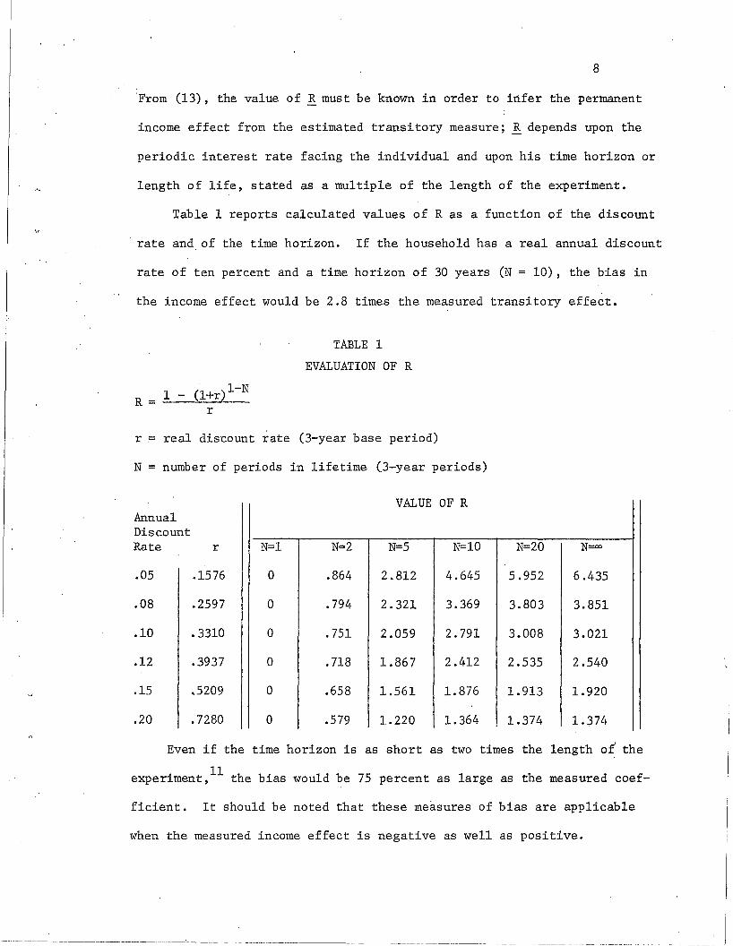
'From (13), the value of R must be known in order to infer the permanent

income effect from the estimated transitory measure; R depends upon the

periodic interest rate facing the individual and upon his time horizon or

length of life, stated as a multiple of the length of the experiment.

Table 1 reports calculated values of R as a function of the discount

rate and of the time horizon. If the household has a real annual discount

rate of ten percent and a time horizon of 30 years (N = 10), the bias in

the income effect would be 2.8 times the measured transitory effect.

TABLE 1

EVALUATION OF R

1 - (l+r)l-NR =

r

r = real discount rate (3-year base period)

N = number of periods in lifetime (3-year periods)

VALUE OF RAnnualDiscountRate r N=l N=2 N=5 N=lO N=20 N=CXl

.05 .1576 0 .864 2.812 4.645 5.952 6.435

.08 .2597 0 .794 2.321 3.369 3.803 3.851

.10 .3310 0 .751 2.059 2.791 3.008 3.021

.12 .3937 0 .718 1.867 2.412 2.535 2.540

.15 .5209 0 .658 1.561 1.876 1.913 1.920

.20 .7280 0 .579 1.220 1.364 1.374 1.374

Even if the time horizon is as short as two times the length of the

. 11 h b . ld b 75 1 h d fexper~ment, t e ~as wou e percent as arge as t e measure coe-

ficient. It should be noted that these measures of bias are applicable

when the measured income effect is negative as well as positive.

--------------------------------------------

9

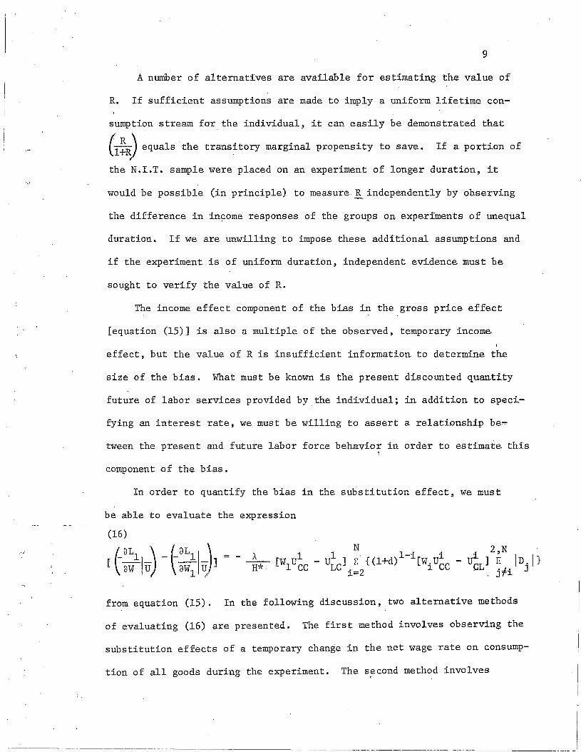
A number of alternatives are available for estimating the value of

R. If sufficient assumptions are made to imply a uniform lifetime con-

sumption stream for, the individual, it can easily be demonstrated that

(l~R) equals the transitory marginal propensity to save. If a portion of

the N.I.T. sample were placed on an experiment of longer duration, it

would be possible (in principle) to measure R independently by observing

the difference in income responses of the groups on experiments of unequal

duration. If we are unwilling to impose these additional assumptions and

if the experiment is of uniform duration, independent evi.dence must be

sought to verify the value of R.

The income effect component of the bias in the gross price effect

[equation (15)J is also a multiple of the observed, temporary income

effect, but the value of R is insufficient information to determine the

size of the bias. What must be known is the present discounted ~uantity

future of labor services provided by the individual; in addition to speci-

fying an interest rate, we must be willing to assert a relationship be~

tween the present and future labor force behavior in order to estimate this1

component of the bias.

In order to quantify the bias in the substitution effect, we must

be able to evaluate the expression

(16)

[t:~llu) -t:~~lu} =A.H*

. 2,Nul.

CL] II In. I}

• ..J.. J. JTl.

from equation (15). In the following discussion, two alternative methods

of evaluating (16) are presented. The first method involves observing the

substitution effects of a temporary change in the net wage rate on consump-

tion of all goods during the experiment. The second method involvesI

. --_.__._--------------

,"

10

placing restrict'ions on the fonn of the singl~ period utility function

(U~) and calculating (16) as a function of marginal budget shares

expended on cash consumption and leisure.

In the single period optimization problem of part I we can state

the conventional adding-up condition from neoclassical consumption

theory that the price-weighted sum of substitution effects of a single

price change across all goods eq~als zero:

(17) 3C I3W U + W31,-= 03W

In the multiperiod model of part II we are concerned with a first

period change in the wage rate resulting from the experiment. The

adding-up condition comparable to (17) places a zero restriction on

the price-weighted substitution effects summed over all time periods,

but places no restriction on the substitution effects summed only over

the period of the experiment. The deviation of this sum from zero is

directly related to the substitution bias in (16).

After differentiating (9)

weighted sum of (_ 3111_) andI 3W U

1

(18)

'3LI 3C11{-W1 3w

llu - 3W

lU} =

to obtain compensated price effects, the

(

3111 ~ can be written as- 3Wl ~

which is positive or negative depending upon whether leisure is a

normal or an inferior good during the experimental period.

The importance of the present discounted quanti.ty of future labor

services in detennining the income effect component of the bias in the

gross price effects was mentioned above; similarly, the marginal share

of leisure in future consumption is the remaing element needed to

quantify the substitution bias. Again, differentiating (9), we obtain

I

I

II

I

I

I

/

"i(

I\ 11

II

(1+dri i . 1,M'

- l+r [WiUCC - UJ. ] II /1 n. I(19) aL. LC (J

J. Hi and=aG1 IH*I

i\

,~

, 'l-i 1 1 N(1~) [/J.lrrln,IJ

ac, aL. r . J. '#' J':--; I J J.

(20) J. ' J. I[W + Wi aG1J =

IH*li

1

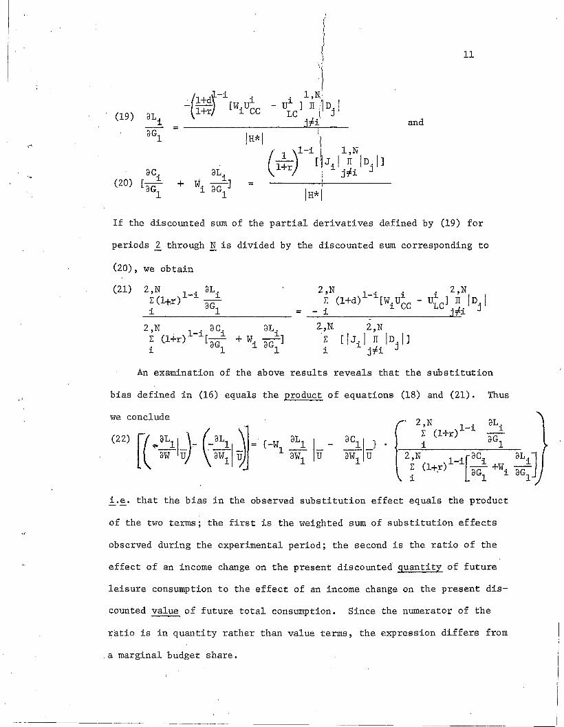
If the discounted sum of the partial derivatives defined by (19) for

periods 1 through N is divided by the discounted sum corresponding to

(20), we obtain

(21) 2,N l' aL.-J. J.~ (l+-d aG

1 =

2.,N. 2,NL; [IJ.I II In,l]i J. j#i J

"

An examination of the above results reveals that the substitution

bias defined in (16) equals the product of equations (18) and (21). Thus

we conclude

(22)

, 2,N l' aL.L; (l+r) -J. J.i aG1

2,N 1 ,[ac~ aL'J-J. J. J.~ (l+.r) aG

1+Wi aG

1

i.e. that the bias in the observed substitution effect equals the product

of the two terms; the first is the weighted sum of substitution effects

observed during the experimental period; the second is the ratio of the

effect of an income change on the present discounted quantity of future

leisure consumption to the effect of an income change on the present dis-

counted value of future total consumption. Since the numerator of the

ratio is in quantity rather than value terms, the expression di.ffers from

,a marginal budget share.

._~--------_._---_._------~---~----------

12

Evaluation of the substitution bias requires some estimate of

future leisure consumption. If we were to impose the additional res-

trictions cited in part II as being sufficient to guarantee a uniform

life-time consumption stream [i.e. ~ = ~' Ui (.) identical for all time

periods, and fixed relative prices through time], the ratio required

in (22) would equal the corresponding ratio observed during the exper-

imental period. The same result would hold with i ~ ~' if we were to

iadd the requirement that U (.) be homogeneous. It should be emphasized,

however, that so long as the assumptions of our more general model are

fulfilled, failure of the more stringent restrictions to hold affects

our ability to estimate the substitution bias only insofar as it affects

the accuracy of our estimate of the relative future consumption of

leisure. A given error in the estimated value of the ratio in (22)

translates into an equal percentage error in the estimated substitution

bias. Failure to estimate the appropriate market interest rate or the

time horizon of the individual plays precisely the same role. It

should be noted that the fact that relative leisure consumption increases

substantially after an individual reaches retirement age does not have a

major impact on the appropriateness of using current leisure behavior

as an approximation of discounted future behavior, since consumption

patterns in the distant future are presumably discounted heavily.

While the expression in (22) is directly measurable, given assump-

tions about the relationship between present and future leisure

consumption, it provides no intuitive assessment of the relative magni-

tude of the substitution bias. By again placing further

\": "

" 'j

, "I. ~ ..' :'! .

13

restrictions on the form of the utility function, we can state the'

ratio of the transitory and permanent substitution effects in terms

of the marginal shares of expenditures on leisure and cash consump-

tion.

Reevaluating the components of (22), the first element drawn

from equation (18) can be written as

(23)

where MPS is the marginal propensity to save observed during the exper-

. 1 . d 12J.menta perJ.o • If, in addition, we impose the approximation that

(24) 2,N l' aL.-J. J.~ (l.+r) aG

l2,N 1 ,[ac,-J. J.~ (l+r) aG

l+ WI :~~J

'V -::----=---- =

equation (22) can be rewritten as

(25)

[t :~llu) -(- :~~I~] ~_ Ul ]2

LC

If we now impose the restrictions that d = r, that prices are

uniform across time, and ,that Ui (.) is identical in every time period

and additive within as well as acrossaLl A. '

results that - aw I U = ~ and

1 1 2 W 2 1(26) "[WIUCC - ULC ] = 1 UCC

III 1 1[UCCULL - UCLULC ] U

LL

time periods, we can utilize the

14

to obtain

(27) L(- :~llu)

~ :~llu )(MPS) •

Thus the substitution bias as a proportion of the permanent substitution

effect equals the product of the observed marginal propensity to save

~nd the ratio of marginal budget shares expended on leisure and cash

. . h .. d 13consumpt~on, g~ven t e restr~ct~ons state .I

In section III we identified the bias in the income effect to be

a function of R, which is a function of the interest rate and the

time horizon of the household. The bias in the substitution effect

can be identified by measuring the weighted sum of single period

substitution effects, and by approximating future relative leisure

consumption; under more stringent restrictions, the substitution bias

depends upon the marginal propensity to save and marginal budget shares.

The results of this paper can easily be extended to a model with

mogoods. The reported results concerning income effects can be gener-

a1ized directly to the multigood case. The biases in the substitution

effects of a price change on any two goods can be shown to be propor-

tiona1 to the effects of an income change on consumption of the two

14goods. If an approximation such as (24) holds as an equality for

the good undergoing the price change, the price-weighted sum of sub-

stitution biases will equal the deviation of the observed sum of

substitution effects from zero.

15

IV

The above analysi"s- concerns- a si:tuation in which there exists a

desire to make inferences about permanent behavioral relationships

from measurements of behavior generated from a temporary experiment.

The converse problem exists in many discussions of the use of fiscal

instruments, where policy makers may wish to predict the effect of

temporary fiscal measures, based upon the observed empirical effects

of earlier' fiscal measures which were viewed to be permanent. For

example, if one used evidence drawn from the 1964 reduction in U.S.

Personal Income Tax rates (viewed to be permanent) to predict the

effect on consumption of the. 1968 Income Tax Surcharge (viewed to be

temporary) one would expect the income effect of the 1968 Surcharge

to have been substantially overestimated.. The permanent income

hypothesis has been widely cited in making this argument concerning

the effects of temporary changes in income tax rates; the analysis

of income effects in this paper corresponds to the implications of

. the permanent income hypothesis.

Furthermore, the analysis of this paper suggests that temporary

fiscal measures which affect the prices faced by decisionmakers (such

as investment credits, excise taxes on consumer durables, and general

sales or expenditure taxes) will have a stronger effect on short-run

behavior than would be predi.cted from empirical ·measures of responses

to price changes viewed to be permanent. This paper suggests procedures

for predicting the strength of such fiscal measures. The reader must

be cautioned, h9wever, that this paper, as a partial equilibrium analysis,

stops far short of making pr'edictions about the general equilibrium

or macroeconomic magnitude of such measures.

II

II

...'. ; r· .',,. j.

16

At least three critical assumptions implied in the above analysis

would, if relaxed, create mitigating complications in the reported

results. First, it is assumed that the households in question face

perfect capital and labor markets. The nature of borrowing and labor

market constraints facing low income households, and the expected

impact of these constraints on behavior, must be investigated before

considering seriously either the results of current negative income

tax experiments or the measures of bias in those results suggested in

this paper. Second, it is assumed that the households in question

adjust instantaneously and costlessly to changes in their economic

·environment. Again, the magnitude of adjustment costs and lags must

be investigated. Finally, it is assumed that the households behave

as if they know with certainty the duration of the experiment. Given

the possibility that households may expect a negative income tax

similar to the experiment~l tax to be permanently enacted prior to

the end of the experiment, and given that the conductors of the

experiment may have obscured its duration in the minds of the parti-

cipating households, the effects of uncertainty and of different

patterns of ~xpectations on behavior must also be accounted for.

17

NOTES

1. In addition to the New Jersey - Pennsylvania Graduated WorkIncentive Experiment and the Rural Graduated Work IncentiveExperiment (Iowa-North Carolina) funded through the Office ofEconomic Opportunity, 'similar experiments are operating or in theplanning stages in Gary, Seattle, and Denver.

2. The terms "individual" and "household" are used interchangeablyin this paper. The household is assumed to possess a singledecision maker and to have a finite lifetime corresponding to,that of the decision maker.

3. We are abstracting from all problems related to sample designand stochastic estimation. The analysis of this paper is donein a nonstochastic framework. For a discussion of sample designprocedures in such experiments, see Orcutt and Orcutt [3], andConlisk and Watts [1].

4. For expositional purposes, we now treat the income guarantee asthe only source of nonwage income.

5. The individual is assumed to have no bequest motive;, he derivesutility only from his own consumption.

6. We can interpret the individual's "lifetime" as being that portionof his life commencing with the initiation of the negative incometax. Given the form of (7), behavior prior to "period 1" affectsbehavior during the period of analysis only through its effect onthe budget constraint.

7. It should be noted that

(a)

IH*IN

= L:

i=l

N(IJ.I II ID.I)

~, Jj:ri> °

Additional requirements implied by the ~econd order conditons foroptimization include

(b) IJ. I > 0, all i, and~

(c) '{ IJ. I. ID. I + IJ . I ·1 D. I} > 0, all i j, i:lj~,J J ~

Conditions (b) and (c) imply that 'In.l have a nonpositive value forat most one j. If IDj/. is positive for all j, an increase in thepresent value of the individual's income stream will increase totalexpenditures in every time period. If IDjl is negative for one j,an increase in the present 'value of income wil), lead to an increasein expenditures in all other periods. (If IDj I = 0 for one j, ex­penditures would increasa in per£od j and remain constant in allother periods) . In this paper i.t is assumed"tIiat /.Dj I. > 0 for all j,

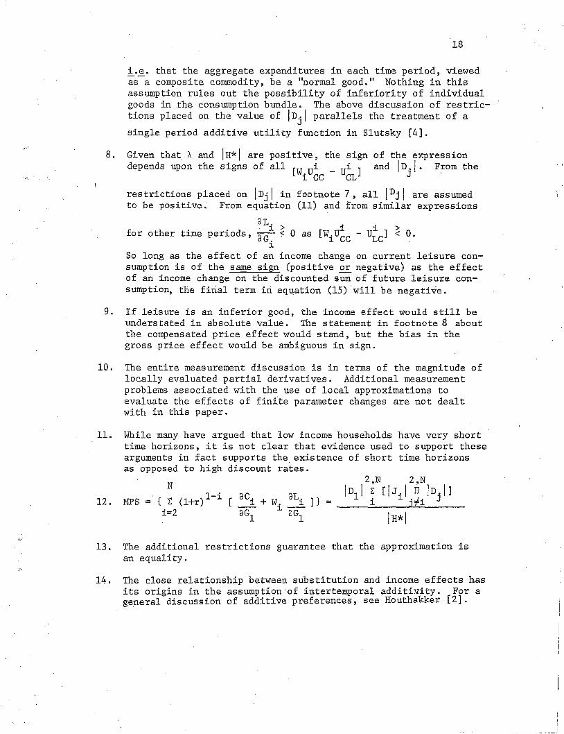
18

Le. that the aggregate expenditures in each time period, viewedas a composite commodity, be a "normal good." Nothing in thisassumption rules out the possibility of inferiority of individualgoods in the consumption bundle. The above discussion of restric­tions placed on the value of fDjl parallels the treatment of a

single period additive utility function in Slutsky [4].

Given that A and IH*I aredepends upon the signs of

8. positive, the sign of the expressionall [W Ui _ Ui ] and ID.I· F~om the

i CC CL J

restrictions placed on [Djl in footnote 7, all [Djl are assumedto be positive. From equation (11) and from similar expressions

ClL. •.. ' 1 > 11>

for other time per10ds, ClG. ~ a as [WiUCC - ULC ] < ~.

1

So long as the effect of an income change on current leisure con­sumption is of the same sign (positive or negative) as the effectof an income change on the discounted sum of future leisure con­sumption, the firial term iri eq~ation (15) 'will be negative.

9. If leisure is an inferior good, the income effect would still beunderstated in absolute value. The statement in footnote 8 aboutthe compensated price effect would stand, but the bias in thegross price effect would be ambiguous in sign.

10. The entire measurement discussion is in terms of the magnitude oflocally evaluated partial derivatives. Additional measurementproblems associated with the use of local approximations toevaluate the effects of fin{te parameter changes are not dealtwith it). this paper.

11. While many have argued that low income households have very shorttime horizons, it is not clear that evidence used to support thesearguments in fact supports the, existence of short time horizonsas opposed to high discount rates.

N

12. MPS =' { ! (l+r)l-ii=2

2,N 2,N

C " IDII l:. [I J.; I ':fIT. IDJ. I]Cl i + W. oLi ]} = ~__ 1 __ _ 1 ....J"-'-1 _

ClGl ClGl IH*I

13. The additional restrictions guarantee that the approximation isan equality.

14. The close relationship between substitution and income effects hasits origins in the assumption 'of intertemporal additi~ity. For a~eneral discussion of additive preferences, see Houthakker [2].

(_.

19

REFERENCES

[1] J. Conlisk and H. Watts, "A Model for Optimizing ExperimentalDesigns for Estimating Response Surfaces," 1969 Proceedings ofthe Social Statistics Section, American Statistical Association,pp. 150-156.

[2] H.S. Houthakker, "Additive Preferences," Econometrica 28(April 1960): pp. 244-256.

[3] G.H. Orcutt and A.G. Orcutt, "Incentive and DisincentiveExperimentation for Income Maintenance Policy Purposes,"The American Economic Review 58 (September 1968): pp. 754-772.

[4] Eugen E. Slutsky, "On the Theory of the Budget of the 'Consumer,"Giornale degli Economisti, Vol. LI (1915), pp. 1-26, reprintedin American Economic Association, Readings in Price Theory,(Homewood, Illinois, 1952): pp. 27-56.