Income and Expenditure Accounts technical series

Chain Fisher Volume IndexMethodologyby Michel Chevalier

Income and Expenditure Accounts Division21st Floor, R.H. Coats Building, Ottawa, K1A 0T6

Telephone: 1 613 951-3640

This paper represents the views of the author and does not necessarily reflect the opinions of Statistics Canada.

Canada

Income and Expenditure Accounts technical series

Catalogue no. 13-604-MIE — No. 42

ISSN: 1707-1739

ISBN: 0-662-35296-3

Research Paper

On May 31, 2001 the quarterly income and expenditure accounts adopted the Fisher index formula,chained quarterly, as the official measure of real gross domestic product in terms of expenditures. This formulawas also adopted for the Provincial Accounts on October 31, 2002.

There were two reasons for adopting this formula: to provide users with a more accurate measure of realGDP growth between two consecutive periods and to make the Canadian measure comparable with theIncome and Product Accounts of the United States, which has used the chain Fisher index formula since 1996to measure real GDP.

OttawaNovember 2003

Catalogue no. 13-604-MIE no. 42ISBN: 0-662-35296-3ISSN: 1707-1739

Catalogue no. 13-604-MPE no. 42ISBN: 0-662-35295-5ISSN: 1707-1720

Published by authority of the Minister responsible for Statistics Canada

© Minister of Industry, 2003

All rights reserved. No part of this publication may be reproduced, stored in a retrieval system or transmittedin any form or by any means, electronic, mechanical, photocopying, recording or otherwise without prior writtenpermission from Licence Services, Marketing Division, Statistics Canada, Ottawa, Ontario, Canada K1A 0T6.

The paper used in this publication meets the minimum requirements of American National Standard forInformation Sciences - Permanence of Paper for Printed Library Materials, ANSI Z39.48 - 1984.

Chain Fisher Volume Index Methodology


Statistics Canada – Catalogue no. 13-604-MIE no. 42 i

Table of contents 1.0 Introduction ......................................................................................................................................... 1 2.0 Building an index and chaining .......................................................................................................... 1

Example 1 : A wine and cheese economy ............................................................................................. 2 Example 2 : Wine and cheese production without the price effect ........................................................ 3 Example 3 : Another way to remove the price effect ............................................................................. 4

3.0 Choice of index..................................................................................................................................... 5 4.0 Application in the Income and Expenditure Accounts..................................................................... 6

Example 4 : In the real world : the deflation method.............................................................................. 7

4.1 Annual and quarterly National Economic and Financial Accounts.......................................... 9 Level of detail at the national level................................................................................................... 9

4.2 The problem of inventory.............................................................................................................. 9 4.3 The provincial accounts.............................................................................................................. 10

Level of detail at the provincial level .............................................................................................. 10 Sources of bias between the national and the provincial systems................................................ 11

5.0 The problem of non-additivity........................................................................................................... 11

Contribution to a GDP change series................................................................................................... 12 Appendix I: Transformation of Laspeyres and Paasche indexes........................................................ 13 Appendix II: Contribution to change formula ........................................................................................ 14 Bibliography .............................................................................................................................................. 17 Technical series ........................................................................................................................................ 19


Statistics Canada – Catalogue no. 13-604-MIE no. 42 1

Chain Fisher Volume Index Methodology by Michel Chevalier

1.0 Introduction

Growth in the current gross domestic product (GDP) or any other nominal value aggregate can be decomposed into two elements: a “price effect”, or the part of the growth linked to inflation, and a “volume effect”, which covers the change in quantities, quality and composition of the aggregate. The volume effect is presented in the National Accounts by what is referred to as the “real” series (such as the real GDP). In the Canadian National Accounts, the volume effect is determined using the deflation method, which eliminates the price effect from each component of the aggregate and then aggregates the components thus deflated to obtain the “total” volume effect. There are several ways to aggregate the components of an aggregate in order to calculate the volume effect. Index number theory offers a wide range of tools to this end. Since spring 2001, Statistics Canada has preferred the chain Fisher index. This measure is theoretically superior to the former fixed-base Laspeyres measure and also makes the Canadian data comparable with the United States’ official measures of economic activity. Furthermore, it offers compliance with the recommendations of the System of National Accounts 1993 (SNA).1 The following paragraphs provide a simplified explanation of the methods that will henceforth be used by the National Accounts to measure the country’s real economic activity.

2.0 Building an index and chaining

A given nominal aggregate (GDP or other) represents a summation of quantities evaluated in the same monetary unit, at the prices of the current period. To use GDP as an example, this summation can be expressed as GDP = Σpq , which is the sum of all quantities of goods and services transacted in the economy, multiplied by their respective prices. The change or variation in nominal GDP, between a period o and a period t, can therefore be expressed in index2 form by:

(1) ∑∑=∆

oo

ttot qp

qpGDP /

where: ∆GDPt/o is the GDP variation index pt is the price at time t p0 is the price at time o qt is the quantity at time t qo is the quantity at time o

1 System of National Accounts 1993. Prepared under the auspices of the Inter-Secretariat Working Group on National Accounts: Commission of the European Communities – Eurostat; International Monetary Fund; Organisation for Economic Co-operation and Development; United Nations; World Bank. Brussels/Luxembourg, New York, Paris, Washington, D.C., 1993. 2 That is, by establishing a ratio between the size of the current period and the size of a preceding period.


2 Statistics Canada – Catalogue no. 13-604-MIE no. 42

A calculation of a GDP value index is shown in Example 1: A wine and cheese economy. The change obtained by this formula may theoretically be divided into a change in prices and a change in volume. If there were an “average” GDP price then it would be quite simple to divide the change in GDP (given by Equation (1)) by this average price to obtain the average change in quantities. Most of the time in the National Accounts, there is no such average price. Thus, the total change in quantities can only be calculated by adding the changes in quantities in the economy. However, creating such a summation is problematic in that it is not possible to add quantities with physically different units, such as cars and telephones, even two different models of cars. This means that the quantities have to be re-evaluated using a common unit. In a currency-based economy, the simplest solution is to express quantities in monetary terms: once evaluated, that is, multiplied by their prices, quantities can be easily aggregated.

Example 1: A wine and cheese economy… In an insular economy where there would be only wine and cheese, we find the following portrait of production for the last four quarters :

Q1 Q2 Q3 Q4 q 100 105 108 112 p 15 16 18 20

Cheese (kilos)

v 1,500 1,680 1,944 2,240 q 25 30 38 50 p 22 20 16 12

Wine (liters)

v 550 600 608 600 Total GDP v 2,050 2,280 2,552 2,840

In this economy, the quantity of cheese produced rises regularly, as well as its price. However, the quantity of wine produced raises very quickly as its price drops significantly. What would the growth of the nominal GDP be between, say, Q1 and Q3? The calculation of the index defined by the equation (1) gives the answer:

245.1050,2

552,2

)2225()15100(

)1638()18108(

11

331/3 ==

×+××+×==∆

∑∑

QQ

QQQQ

qp

qpGDP

The growth of the economy, in nominal terms, will therefore be 24.5% between Q1 and Q3 (we get the percentage growth by subtracting 1 from the ratio given by the index and by multiplying the result by 100). This calculation can be done for all the periods relative to Q1. At the end, we obtain an index that covers the four periods :

Q1 Q2 Q3 Q4 ∆GDP i 1.000 1.090 1.245 1.385

What would the growth be between periods Q3 and Q4? Here, the ratio of the indexes in Q3 and Q4 gives the answer :

112.1245.1

385.13/4 ==∆ QQGDP

The growth will therefore be 11.2% between periods Q3 and Q4.

An intuitive way to measure changes in quantity over time is to take the prices available for a given period and to multiply the quantities from the subsequent periods by these same prices. It amounts to re-evaluating current quantities at prices fixed in time, which essentially “removes” the price effect. In mathematical terms, this can be expressed by the formula for the fixed-base Laspeyres index:

(2) ∑∑=

oo

toot qp

qpLQ /



where: LQt/o is the Laspeyres quantity index

p0 is the price at time o qt is the quantity at time t qo is the quantity at o The only difference from Equation (1) is found in the numerator, where the quantities at time t are multiplied this time by the prices at time o. An application of this formula is shown in Example 2: Wine and cheese production without the price effect. It is quite clear with such a formula that the results are highly dependent on the structure of prices at time o. Should this structure change with time, for example as a result of a drop in the price of one component compared with the others, then the index from Equation (2) will eventually be biased by the fact that it is dependent on an outdated price structure. One way to overcome this type of problem is to periodically update the weighting base to bring it in line with the current period. This technique was used in the past by the System of National Accounts (SNA) when the real series was rebased every five or six years to reflect changes in the price structure.

Example 2 : Wine and cheese production without the price effect… Still using our wine and cheese economy, this time we want to evaluate the increase in GDP between period Q1 and periods Q2, Q3 and Q4, excluding the price effect. In our table of the economy, we will use the prices in Q1 as « fixed prices » :

Q1 Q2 Q3 Q4 q 100 105 108 112 p 15 16 18 20

Cheese (kilograms)

1,500 1,680 1,944 2,240 q 25 30 38 50 p 22 20 16 12

Wine (liters)

550 600 608 600 Total GDP 2,050 2,280 2,552 2,840

Applying equation (2), we obtain, for the growth between Q1 and Q3 :

198.1050,2

456,2

)2225()15100(

)2238()15108(

11

311/3 ==

×+××+×==

∑∑

QQ

QQQQ

qp

qpLQ

The growth in real GDP is 19.8% between Q1 and Q3. The same index can be calculated for all of the periods, still using Q1 as a base :

Q1 Q2 Q3 Q4 LQt/Q1 i 1.000 1.090 1.198 1.356

This time, the growth between periods Q3 and Q4, excluding the price effect, is 13.2% :

132.1198.1

356.13/4 ==∆ QQLQ

It is noteworthy that this growth of real GDP between Q3 and Q4 is greater than the growth in nominal GDP, which is 11.2%. According to this fixed-base Laspeyres index, the implicit price of the GDP, i.e. the nominal GDP divided by the real GDP (we also call it the general level of prices), has therefore dropped between Q3 and Q4.



It is possible, however, for the price structure to change more quickly that usual. The weighting base then becomes outdated quickly, perhaps making it necessary to increase the frequency of the rebasing. Ultimately, the weighting base can be systematically moved from period to period so that it is defined as being the period preceding the current period:

(3) ∑∑

−−

−− =

11

11/

tt

tttt qp

qpLQ

where we find, in place of po from Equation (2), pt-1. For the current period t, this “mobile-base” index gives the growth in volume weighted according to prices t-1. To some extent it incorporates the frequency of the rebasing, thereby eliminating the arbitrariness of a rebasing done only on an “as required” basis.

Example 3: Another way to remove the price effect In the previous example, the growth in GDP between Q3 and Q4 was evaluated using Q1 prices. However, with time a change in the price structure of our isolated economy is becoming evident : the liter of wine, more expensive than the kilogram of cheese in Q1, becomes less expensive by Q3. Thus, this time, we will measure the growth between Q3 and Q4 using Q3 prices as the base.

Q1 Q2 Q3 Q4 q 100 105 108 112 p 15 16 18 20

Cheese (kilograms)

1,500 1,680 1,944 2,240 q 25 30 38 50 p 22 20 16 12

Wine (liters)

550 600 608 600 Total GDP 2,050 2,280 2,552 2,840

Applying equation (3) gives us :

103.1552,2

816,2

)1638()18108(

)1650()18112(

33

433/4 ==

×+××+×==

∑∑

QQ

QQQQ

qp

qpLQ

The growth in real GDP is now evaluated at 10.3% between Q3 and Q4, rather than 13.1% with the fixed-based Laspeyres index. What happened? The change in quantities in the previous box were evaluated using a different price structure : the change in production from 38 to 50 liters of wine was evaluated at 22$/litre, while now this increase in production is evaluated at 16$/litre. The increase in « quantity » thus carries less weight in the balance when the aggregation is done. What would be the growth between Q1 and Q3? Since equation (3) measures only the relationship between the current and the previous period, we cannot deduct this directly from this equation. However, we can multiply the successive growth of each period between Q1 and Q3. For example, if the growth is 2.3% between Q1 and Q2 and 4.3% between Q2 and Q3, the growth between Q1 and Q3 will be 1.023 X 1.043 = 1.067, so 6.7%. This calculation, the same as that of compound interest, illustrates the principle of chaining. Applied to our economy, equations (3) and (4) give us :

Q1 Q2 Q3 Q4 Unchained Laspeyres index 1.000 1.090 1.091 1.103 Chained Laspeyres index 1.000 1.090 1.190 1.313

The growth between Q1 and Q3 will therefore be 19.0% :

190.1000.1

190.11/3 ==∆ QQLQ



In the short term, this type of index can be adapted to cover several periods. Equation (3) can be chained by successive multiplications, that is, in each period, it can be multiplied by the results obtained from the preceding period. The prices used for weighting in the resulting chain are very recent prices and never become obsolete. Using our example, a chain index would have the following form:

(4) ∑∑

∑∑

∑∑

∑∑

−−

−

−−

− ×××××=11

1

11

1

11

211 ......nn

nn

tt

tt

oo

oC qp

qp

qp

qp

qp

qp

qp

qpLQ

where n is the number of periods over which the chain index extends. Example 3 : Another way to remove the price effect shows how such a formula can be used. The System of National Accounts, 1993 recommends using chain indexes. Statistics Canada has been following this recommendation since the spring of 2001 for quarterly National Accounts and since the fall of 2002 for the Provincial Economic Accounts. Systematic chaining allows for constant renewal of the weighting base, thus avoiding the problem of outdated data associated with a fixed-base index.

3.0 Choice of index

The previous examples refer to a Laspeyres-type index. However, index number theory provides numerous other indices that differ in the way the components are weighted. For example, although the quantities in the Laspeyres index are weighted with the prices of a previous period, in the Paasche index they are weighted with the prices of the current period:

(5) ∑∑=

ot

ttot qp

qpPQ /

where PQt/o is the Paasche quantity index. This index is in fact the reciprocal of the Laspeyres index. Used in its fixed-base form, it presents the same problem as that described earlier, but the inverse: it does not adequately reflect changes in the structure of the economy for previous periods. However, the Paasche index can be chained in the same way as the Laspeyres index (as in Equation (4)). It can be shown that, in general, a Laspeyres quantity index will generate a larger increase over time than a Paasche quantity index. This occurs when prices and quantities are negatively correlated, that is, when goods or services that had become relatively more expensive are replaced by goods and services that have become relatively less expensive. This common substitution effect says to economic theory that the Laspeyres and Paasche indexes set upper and lower limits for a theoretically ideal, less biased, index. This theoretical index can be approached by a Fisher-type index, representing the geometric mean of a Laspeyres and Paasche index:

(6) ∑∑

∑∑ ×=×=

ot

tt

oo

toototot qp

qp

qp

qpPQLQFQ ///

where FQt/o is the Fisher quantity index. This index is not only superior theoretically, but it also includes a number of desirable properties from the standpoint of the National Accounts. For example, it is “reversible over time”, that is, the index showing the change between period o and period t is the reciprocal of the index showing the change between period t and period o. Another interesting feature is the “reversibility of factors” by which the product of the price and quantity indexes is equal to the index of the change in current values:

∑∑

∑∑

∑∑

∑∑

∑∑ =×××=×

oo

tt

ot

tt

oo

to

to

tt

oo

ototot qp

qp

qp

qp

qp

qp

qp

qp

qp

qpFQFP //



This brings us back to our index of nominal change in Equation (1) and the decomposition of the “price effect” and “volume effect” discussed at the start of this paper. From there, it is quite easy to find the implicit Fisher price of GDP by dividing GDP in current dollars by real GDP using the Fisher formula. The Laspeyres and Paasche indexes do not have either of these two properties. The Income and Expenditure Accounts use the chain Fisher index as a measure of real GDP. Following the same sequence that we used with Equation (4), chaining Equation (6) gives us:

(7)∑∑

∑∑

∑∑

∑∑

∑∑

∑∑

−−−

−

−−−

− ×××××××=111

1

111

1

1

111 ......nn

nn

nn

nn

tt

tt

tt

tt

ooo

oC qp

qp

qp

qp

qp

qp

qp

qp

qp

qp

qp

qpFQ

This is the formula used as the basis of the calculations of real GDP for the National and Provincial Accounts.

4.0 Application to the Income and Expenditure Accounts

In practice, the formulae provided above cannot be used as is, given the absence of data on quantities and price levels. The Accounts have only current value (C) series and price indexes (thus, relative prices). Formulas have to be transformed using the fact that the price multiplied by the quantity (ptqt) equals the series in current dollars (Ct). We then get formulae expressed in terms of nominal series (Ct) and relative prices (pt/pt-1 or the reverse). This then gives us, for Laspeyres (using Equation (3)):

(8) ∑

∑−

−

−

=1

1

1/t

tt

t

tt C

Cp

p

LV

… for Paasche (using Equation (5)):

(9)

∑

∑

−−

−

=

11

1/

tt

t

ttt

Cp

p

CPV

… and lastly, for Fisher (geometric mean of Equations (8) and (9)):

(10)

∑∑

∑∑

−−

−

−

−

×

=

11

1

1

1/

tt

t

t

t

tt

t

tt

Cp

p

C

C

Cp

p

FV

It is this formula, chained, that is used in practice. The detail of the transformations can be examined in Appendix I. Since the series are no longer expressed in terms of quantities, we will now refer to them as volume index. The concept of volume is broader than that of quantity, because it includes variations in quality and ultimately, changes in the composition of the economy.



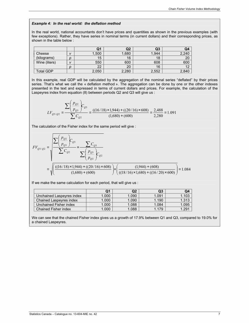
Example 4: In the real world: the deflation method In the real world, national accountants don’t have prices and quantities as shown in the previous examples (with few exceptions). Rather, they have series in nominal terms (in current dollars) and their corresponding prices, as shown in the table below :

Q1 Q2 Q3 Q4 v 1,500 1,680 1,944 2,240 Cheese

(kilograms) p 15 16 18 20 v 550 600 608 600 Wine (liters) p 22 20 16 12

Total GDP 2,050 2,280 2,552 2,840 In this example, real GDP will be calculated by the aggregation of the nominal series “deflated” by their prices series. That’s what we call the « deflation method ». The aggregation can be done by one or the other indexes presented in the text and expressed in terms of current dollars and prices. For example, the calculation of the Laspeyres index from equation (8) between periods Q2 and Q3 will give us :

091.1280,2488,2

)600()680,1()608)16/20(()944,1)18/16((

2

33

2

2/3 ==+

×+×=

=∑

∑

Q

QQ

Q

QQC

Cp

p

LV

The calculation of the Fisher index for the same period will give :

084.1)600)20/16(()680,1)16/18((

)608()944,1(

)600()680,1(

)608)16/20(()944,1)18/16((

22

3

3

2

33

2

2/3

=

×+×

+×

+

×+×=

×

=

∑

∑∑

∑

QQ

Q

Q

Q

QQ

Q

QQ

Cp

p

C

C

Cp

p

FV

If we make the same calculation for each period, that will give us :

Q1 Q2 Q3 Q4 Unchained Laspeyres index 1.000 1.090 1.091 1.103 Chained Laspeyres index 1.000 1.090 1.190 1.313 Unchained Fisher index 1.000 1.088 1.084 1.095 Chained Fisher index 1.000 1.088 1.179 1.291

We can see that the chained Fisher index gives us a growth of 17.9% between Q1 and Q3, compared to 19.0% for a chained Laspeyres.



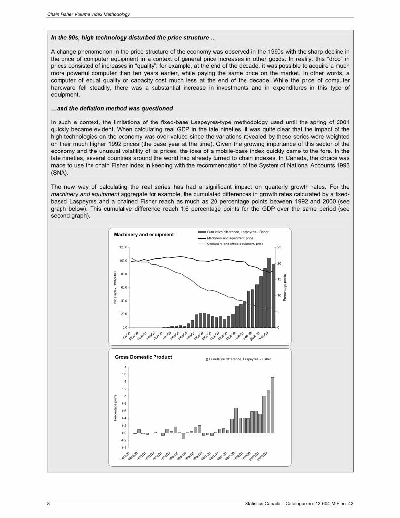
In the 90s, high technology disturbed the price structure … A change phenomenon in the price structure of the economy was observed in the 1990s with the sharp decline in the price of computer equipment in a context of general price increases in other goods. In reality, this “drop” in prices consisted of increases in “quality”: for example, at the end of the decade, it was possible to acquire a much more powerful computer than ten years earlier, while paying the same price on the market. In other words, a computer of equal quality or capacity cost much less at the end of the decade. While the price of computer hardware fell steadily, there was a substantial increase in investments and in expenditures in this type of equipment. …and the deflation method was questioned In such a context, the limitations of the fixed-base Laspeyres-type methodology used until the spring of 2001 quickly became evident. When calculating real GDP in the late nineties, it was quite clear that the impact of the high technologies on the economy was over-valued since the variations revealed by these series were weighted on their much higher 1992 prices (the base year at the time). Given the growing importance of this sector of the economy and the unusual volatility of its prices, the idea of a mobile-base index quickly came to the fore. In the late nineties, several countries around the world had already turned to chain indexes. In Canada, the choice was made to use the chain Fisher index in keeping with the recommendation of the System of National Accounts 1993 (SNA). The new way of calculating the real series has had a significant impact on quarterly growth rates. For the machinery and equipment aggregate for example, the cumulated differences in growth rates calculated by a fixed-based Laspeyres and a chained Fisher reach as much as 20 percentage points between 1992 and 2000 (see graph below). This cumulative difference reach 1.6 percentage points for the GDP over the same period (see second graph).

Machinery and equipment

0.0

20.0

40.0

60.0

80.0

100.0

120.0

1992

Q1

1992

Q3

1993

Q1

1993

Q3

1994

Q1

1994

Q3

1995

Q1

1995

Q3

1996

Q1

1996

Q3

1997

Q1

1997

Q3

1998

Q1

1998

Q3

1999

Q1

1999

Q3

2000

Q1

2000

Q3

Pric

e in

dex,

199

2=10

0

0

5

10

15

20

25

Per

cent

age

poin

ts

Cumulative dif ference, Laspeyres - Fisher

Machinery and equipment, price

Computers and of fice equipment, price

Gross Domestic Product

-0.4

-0.2

0.0

0.2

0.4

0.6

0.8

1.0

1.2

1.4

1.6

1.8

1992

Q1

1992

Q3

1993

Q1

1993

Q3

1994

Q1

1994

Q3

1995

Q1

1995

Q3

1996

Q1

1996

Q3

1997

Q1

1997

Q3

1998

Q1

1998

Q3

1999

Q1

1999

Q3

2000

Q1

2000

Q3

Per

cent

age

poin

ts

Cumulative difference, Laspeyres - Fisher



4.1 Annual and quarterly National

Economic and Financial Accounts

Real aggregates published by the Income and Expenditure Division (IEAD) are calculated using Equation (10) shown above. For each real aggregate, an index is calculated from component series, then chained quarter by quarter as shown in examples 3 and 4. The chained index series thus obtained is then benchmarked to a reference year in order to express it in dollars. Benchmarking consists of putting the level of the chained index series to a level such that, for a given reference year, it is equal to the corresponding aggregate in current dollars, while keeping the quarterly growth rates intact.

What is the difference between the base period and the reference period? The prices used to compile the volume indexes are prices from the base period, while the period in which the value of a series in constant dollars is equal to the value of said series in current dollars is the reference period. In the former real GDP measure, using the fixed-base Laspeyres method, the reference period and the base period were the same. In a chain volume measure, however, the two periods are not necessarily the same. For example, the chain Fisher series in our publication are referenced in 1997 (current dollars equal constant dollars for 1997) but the base corresponds to a combination of the current period and the period immediately before the current period, because it is a chain Fisher index. The reference period serves only to benchmark the series and a change in the reference period does not change any aspect of the growth rates of the series or the aggregates. The only change occurs with the levels, which are benchmarked on a different value.

For this reason, the chain Fisher series currently published cannot be said to be “at 1997 prices”, because the prices of the reference period are not used in any way in the calculation of the quarters preceding or following the reference year. However, it can said that these are series expressed in real terms, thereby easing the price effects, at a level at which they are equal to the nominal aggregate level for 1997. In other words, a real series in which the reference year is 1997 is the equivalent of a nominal series in which the price effect has been removed since 1997.

The level of detail - that is, the number of components used in each of the aggregates - is determined by the availability of data and by certain determinants of overall quality (such as the stability of seasonality). At the national level, 435 series in current dollars and the same number of corresponding price series are used to calculate real GDP using the chain Fisher index. The following table shows how these series are distributed between the various aggregates presented in Table 3 of the publication National Income and Expenditure Accounts, Quarterly Estimates (13-001).

None of the Fisher index calculations are done on an annual basis. The real annual aggregates are simple averages of the year’s four quarters. These are the official measures of real annual national GDP.

4.2 The problem of inventory

For most of the items in publication Table 3 and other tables in real terms, the Fisher calculation does not present any real technical problems. This is not the case for the investment in inventory series, which are first-difference series. Since these series fluctuate around zero, the Laspeyres and Paasche indexes take opposite signs; since Fisher is the geometric mean of these two indexes, it becomes indeterminate.

Table 1: Level of detail at the national level Personal expenditure on consumer goods and services 130 Durable goods 22 Semi-durable goods 15 Non-durable goods 14 Services 79 Government current expenditure on goods and services 24 Government gross fixed capital formation 14 Government investment in inventory 1 Business gross fixed capital formation 18 Residential structures 4 Non-residential structures and equipment 14 Non-residential structures 4 Machinery and equipment 10 Business investment in inventory 110 Non-farm 76 Farm 34 Exports of goods and services 69 Goods 64 Services 5 Imports of goods and services 68 Goods 63 Services 5 Statistical discrepancy 1 Gross domestic product at market prices 435 Final domestic demand 186



As published by the IEAD, real investment in inventories is not the result of a direct chained Fisher calculations as shown above, but rather an approximation. The approach used by the IEAD is based on the fact that an investment in inventory represents the variation of a total stock, which is always positive. In principle, a Fisher index can be calculated on a total stock series. Once this index is benchmarked to the dollar value of a reference year, one can suppose that the first differences of this series, in dollars, represents an estimate of the real series of the investment in inventories. If such a method is easily applicable to the calculation of the real inventory series, it is however unusable in the context of the calculation of real GDP. Indeed, the calculation of real GDP should be done with series of investment in inventories, and not with series of total stock. To bypass this problem, the IEAD uses two series of total stock rather than one for each series of investment in inventories: a first series of the stock in the current period (with a positive sign); and a second series, of the stock in the previous period (with a negative sign). This last series is in fact a series of total stock with a one-period lag. At any time t, the difference between these two series corresponds to the investment in inventories during the same period. If in the GDP we replace every series of investment in inventories by these two series of stocks, one positive and the other negative and lagged, we can calculate the real GDP with the chained Fisher index formula. The prices used for total stocks are those of investment in inventories. The calculation of the real aggregates of investment in inventories involves the same series of total stock. For each aggregate of investment in inventories, a chain Fisher index is obtained from the series of total stock in the current period and another one from the series of the lagged total stock. Once benchmarked to the reference period, these chained Fisher series can be subtracted from each other to simulate a real series of investment in inventories. This is the way that the real aggregates of the investment in inventories are calculated by the Income and Expenditure Accounts Division.

The methodology for calculating the investment in inventory explains the fact that, in Table 1, there are 110 inventory series used in the Fisher calculation, of which 76 are non-agricultural and 34 agricultural (when, in fact, there are 55 inventory series published in current dollars, of which 38 are non-agricultural and 17 agricultural).

4.3 Provincial Accounts

At the provincial level, real values are calculated the same way as they are at the national level, but on an annual basis. Investment in inventory is calculated according to the methodology described above, on an annual basis, with average prices for the year. The level of detail of the provincial accounts differs from that of the quarterly national accounts. For each province, 502 series are used in calculating real GDP. Table 2 shows the distribution of these series through the items in Table 3 of the publication Provincial Economic Accounts (13-213). This distribution is slightly different than the national structure because of the different availability and quality of provincial data.

Table 2: Level of detail at the provincial level Personal expenditure on consumer goods and services 130 Durable goods 22 Semi-durable goods 15 Non-durable goods 14 Services 79 Government current expenditure on goods and services 24 Government gross fixed capital formation 3 Government investment in inventory 1 Business gross fixed capital formation 5 Residential structures 3 Non-residential structures and equipment 2 Non-residential structures 1 Machinery and equipment 1 Business investment in inventory 110 Non-farm 76 Farm 34 Exports of goods and services 114 Exports to other countries 57 Exports to other provinces 57 Imports of goods and services 114 Imports from other countries 57 Imports from other provinces 57 Statistical discrepancy 1 Gross domestic product at market prices 502 Final domestic demand 162



Sources of bias between the national and provincial system The national and provincial systems are additively consistent when expressed in nominal value. However, in real terms, the properties of the chain Fisher index are such that this consistency can no longer be guaranteed. First, real series based on a chain Fisher calculation are not additive. This means that for each province and for Canada as a whole, the sum of the aggregates will not equal the main aggregate (for example, the sum of the aggregates of Table 3 in our publication does not equal GDP). Another consequence of this non-additivity problem is that for each aggregate, the sum of the provinces will not equal the national level (for example, the sum of expenditure on consumer goods and services in all of the provinces will not equal the national expenditure on consumer goods and services). Secondly, real series are calculated differently at the national and provincial levels. While the national annual series represent an average of the quarters, the provincial annual series represent a chain Fisher index calculated on the year. These two different methodologies produce different results. Thirdly, there are theoretically two ways to calculate real series at the national level. Fisher indexes can be calculated with the national series (these being the sum of the provincial series), or calculated directly with the provincial series. Since Fisher is an index sensitive to the number of series involved in the calculation, the two calculations do not produce exactly the same result. Lastly, the level of detail is different between the national and provincial calculations (435 and 502 series, respectively). Since Fisher is an index sensitive to the number of series involved in the calculation, the difference in level of detail produces an inevitable bias between the national and provincial calculation. For these reasons, it is unlikely that the provincial real GDP series will be additively consistent with the national series.

5.0 The problem of non-additivity

The chain Fisher series published by the Income and Expenditure Accounts Division are not additive, and this problem increases with distance from the reference period. Non-additivity of real series comes both from chaining and from the Fisher formula itself. Chaining destroys the additive consistency of accounting equations and the Fisher formula (as opposed to the Laspeyres formula) doesn’t have the additivity property. The fact that the real series are not additive makes them more difficult to manipulate than in the past, when the calculations were based on a fixed-base Laspeyres index. For example, it becomes difficult to measure the contribution of an individual aggregate or sector to a bigger whole knowing that the sum of the aggregates does not add up to the total. It is also imprudent to create aggregates from other aggregates. There are a variety of ways to overcome this additivity problem. For some summary analysis, current dollar data may be enough and even desirable, because they reflect the economic structure at current prices. This is especially true if the aggregates being studied do not exhibit large price variations or if these variations are relatively uniform. For those who want to use real data and create aggregations, one solution is to calculate Fisher indexes using existing Fisher data. Diewert (1978) demonstrated that a Fisher index was approximately consistent, and that therefore it was possible to calculate Fisher indexes from aggregates already in Fisher, what he called a “Fisher of Fishers”. This solution provides a valid approximation provided that the aggregates used in the calculation are relatively consistent in terms of prices (this solution should not be used, for example, if the calculation involves inventory series). A more “structural” solution is to play with the benchmarking frequency. Since additivity decreases with distance from the reference year, rebenchmarking the series to bring the reference year closer may alleviate part of the problem without, however, making the whole strictly additive. It is important to note that, in the case of real data based on chain Fisher index calculations, changing the reference period does not have any impact on the growth rates of real series. Since it is not possible to make the levels additive, the IEAD, following the lead of the Bureau of Economic Analysis in the United States, suggests a strictly additive decomposition of the variations of the aggregates for tables published from real data. The formula used reweights the contributions to the series in such a way that they become strictly additive at the total variation of the aggregate:



(11)

∑ −−

−−

−

×+

−×+×=∆

i

it

t

iti

t

it

it

t

iti

t

tti

qFPpp

qqFPpp

11

11

/1,

)(

)()(100%

Or, in a form that applies to nominal series and to prices,

(11a)

∑ ∑∑

∑

+

−+

−

×

×=∆

−−

−−−

−

−−

i i it

it

ttt

it

iti

titt

iti

t

iti

ti t

i t

tti

ppCFVC

ppCCFVC

ppC

CC

11

111

1

1

/1, 100%

This formula is the basis of the contribution to change series published by the SNA. A detailed mathematical demonstration is available in Appendix II.

Contribution to a GDP change series The contribution of an aggregate to the percentage change in GDP in real terms is presented in Table 4 of the quarterly publication (13-001). Contribution to change tables are also calculated for various grand aggregates (see Tables 18, 21, 24 and 27). Each of these tables follows the layout of the corresponding real data table. Instead of real data, they show the percentage contribution to the variation of the reference aggregate mentioned in the table’s title. For example, Table 4 of our quarterly publication follows the layout of Table 3, and shows the contribution of the aggregates in Table 3 to the percentage growth in real GDP. These contributions are not presented as proportions, but directly as percentage points. For example, a contribution of the aggregate of personal consumption expenditure of 0.453 to real GDP growth of 1.473% means that 0.453 percentage points of the 1.473 are due to personal consumption expenditure.

The formula for percentage contribution to change presented earlier applies only to a single period. To use the same formula over a longer period of time, a Fisher non-chained value is required where the weighting bases correspond to the periods to be analysed. For example, to analyse the growth in durable consumer goods between the fourth quarter of 1996 and the fourth quarter of 2000, it is possible to calculate a Fisher index in which the weighting is explicitly a function of the prices in the fourth quarter of 1996 and of the fourth quarter of 2000. To some degree, it amounts to a fixed-base Fisher index. Once this index has been calculated, the percentage contribution to change formula can be used directly. Users can do such calculations themselves, if they have all of the series included in the aggregate. Otherwise, they can be prepared by Statistics Canada on request.



Appendix I

Transformation of Laspeyres and Paasche indexes

Laspeyres volume index The best known volume index is Laspeyres. For this index, weighting is done using prices from a pre-determined base year.

(1) ∑∑=

oo

to

otqp

qpLQ /

or, in a version that can be chained: (2)

∑∑

−−

−− =

11

11/

tt

tttt qp

qpLQ

where: LQ is the Laspeyres quantity index for period t in relation to period o

p represents the price series q represents the quantity series

By using the identity C = pq (value equals price multiplied by quantity), formula (2) can be expressed in a more usable form:

(3) ∑∑

−−

−

−

=11

1

1/tt

tt

tt

tt qp

qp

pp

LQ

⇒

(4) ∑∑

−−

−

−

=11

1

1/tt

ttt

t

tt qp

qpp

p

LQ

and:

(5) ∑

∑−

−

−

=1

1

1/t

tt

t

tt C

Cp

p

LV

Paasche volume index As well as referring to a previous period, a volume index can be based on prices from the current period. This is known as a Paasche index.

(6) ∑∑=

ot

tt

otqp

qpPQ /

or, in a version that can be chained: (7)

∑∑

−− =

11/

tt

tttt qp

qpPQ

By performing the same substitutions that we did with the Laspeyres index, we get:

(8)

∑∑

−−

−−

=

11

1

1/

tt

tt

tttt

qp

pp

qpPQ

⇒ (9)

∑

∑

−−−

−

=

111

1/

ttt

t

tttt

qpp

p

qpPQ

and: (10)

∑∑

−−

−

=

11

1/

tt

t

ttt

Cp

p

CPV



Appendix II

Contribution to change formula

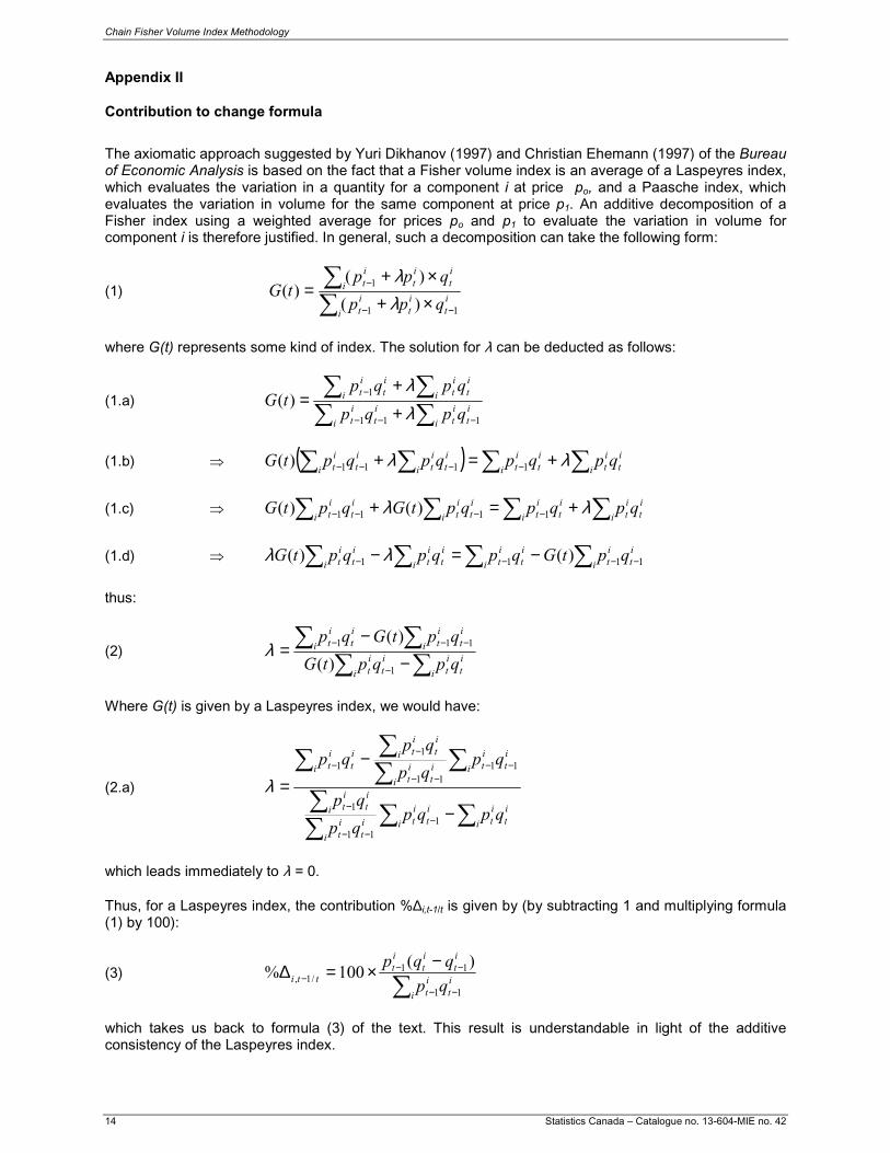
The axiomatic approach suggested by Yuri Dikhanov (1997) and Christian Ehemann (1997) of the Bureau of Economic Analysis is based on the fact that a Fisher volume index is an average of a Laspeyres index, which evaluates the variation in a quantity for a component i at price po, and a Paasche index, which evaluates the variation in volume for the same component at price p1. An additive decomposition of a Fisher index using a weighted average for prices po and p1 to evaluate the variation in volume for component i is therefore justified. In general, such a decomposition can take the following form:

(1) ∑∑

−−

−

×+×+

=i

it

it

it

i

it

it

it

qpp

qpptG

11

1

)(

)()(

λλ

where G(t) represents some kind of index. The solution for λ can be deducted as follows:

(1.a) ∑∑∑∑

−−−

−

++

=i

it

iti

it

it

i

it

iti

it

it

qpqp

qpqptG

111

1)(

λλ

(1.b) ⇒ ( ) ∑∑∑∑ +=+ −−−− i

it

iti

it

iti

it

iti

it

it qpqpqpqptG λλ 1111)(

(1.c) ⇒ ∑∑∑∑ +=+ −−−− i

it

iti

it

iti

it

iti

it

it qpqpqptGqptG λλ 1111 )()(

(1.d) ⇒ ∑∑∑∑ −−−− −=−i

it

iti

it

iti

it

iti

it

it qptGqpqpqptG 1111 )()( λλ

thus:

(2) ∑ ∑

∑∑−

−=

−

−−−

i i

it

it

it

it

i

it

iti

it

it

qpqptG

qptGqp

1

111

)(

)(λ

Where G(t) is given by a Laspeyres index, we would have:

(2.a)

∑ ∑∑∑

∑∑∑∑

−

−=

−−−

−

−−−−

−−

i i

it

it

it

it

i

it

it

i

it

it

i

it

it

i

it

it

i

it

it

i

it

it

qpqpqp

qp

qpqp

qpqp

111

1

1111

11

λ

which leads immediately to λ = 0. Thus, for a Laspeyres index, the contribution %∆i,t-1/t is given by (by subtracting 1 and multiplying formula (1) by 100):

(3) ∑ −−

−−−

−×=∆i

it

it

it

it

it

tti qp

qqp

11

11/1,

)(100%

which takes us back to formula (3) of the text. This result is understandable in light of the additive consistency of the Laspeyres index.



Where G(t) is given by a Fisher index, we have:

(2.b) ∑ ∑

∑∑−

−=

−

−−−

i i

it

it

it

itt

i

it

itti

it

it

qpqpFV

qpFVqp

1

111λ

where FVt is the Fischer volume index at time t. By dividing the numerator and denominator by Σptqt , we obtain:

(2.c)

11

111

−

−=

∑∑

∑∑

∑∑

−

−−−

i

it

it

i

it

it

t

i

it

it

i

it

it

t

i

it

it

i

it

it

qp

qpFV

qp

qpFV

qp

qp

λ

or:

(2.c')

1

1

−

−=

t

t

tt

t

t

PV

FVFPFV

FV

PPλ

where PPt is the Paasche price index at time t, and FPt is the Fisher price index at time t. If we multiply (2.c') by FPt at the numerator and denominator, we obtain:

(2.d) tt

t

t

FPLP

PP

FP

−

−=

1λ

which, multiplied by PPt at the numerator and denominator, becomes:

(2.e) tttt

tt

tt

FPPPLPPP

PPPP

FPPP

−

−=λ

by reducing and using the equivalence PPtLPt = FPt

2, we obtain:

(2.f) ( ) tttt

tt

FPPPFPFP

PPFP 1=−

−=λ



Formula (1) then becomes:

(4)

∑

∑

−−

−

×+

×+=

i

it

t

iti

t

i

it

t

iti

t

t

qFPpp

qFPpp

FV

11

1

)(

)(

To obtain the contribution of a single component to the percentage growth of the aggregate, we take FVt-1 and multiply by 100:

(4.a)

∑ −−

−−

−

×+

−×+×=∆

i

it

t

iti

t

it

it

t

iti

t

tti

qFPpp

qqFPpp

11

11

/1,

)(

)()(100%

This formula is sometimes difficult to operationalize given that it is expressed in terms of price and quantity. For a version expressed in terms of current dollar values and prices (as used by the IEAD), we can multiply the numerator and denominator by FVtFPt:

(4.b)

∑ ∑ −−−

−−−−

−

+

−−+×=∆

i it

it

it

ttit

ittt

t

it

iti

tit

t

it

iti

tittt

tti

FPqpFPFVqpFPFV

FPqpqpFP

qpqpFPFV

111

1111

/1,

)(100%

or:

(4.c) ∑ ∑

∑∑

∑∑

−

−−−

−−

− +

−

−+

×=∆i i

it

ittt

it

itt

it

i t

i titt

it

it

i t

i t

tti qpFVC

qpFVCC

CCFVqp

CC

1

111

11

/1, 100%

by consolidating the sums of the values in current dollars:

(5)

∑ ∑∑

∑

+

−+

−

×

×=∆

−−

−−−

−

−−

i i it

it

ttt

it

iti

titt

iti

t

iti

ti t

i t

tti

ppCFVC

ppCCFVC

ppC

CC

11

111

1

1

/1, 100%



Bibliography Berthier, J.P. (2002), Réflexions sur les différentes notions de volume dans les comptes nationaux, Direction des études et synthèses économique, Institut national de la statistique et des études économiques. Bureau of Economic Analysis (1998), Updated Summary NIPA Methodologies, Survey of Current Business. Bureau of Economic Analysis (1998), National Income and Product Accounts 1929-94 - vol.1, definitions and classifications. Diewert, W.E. (1978), Superlative Index Numbers and Consistency in Aggregation, Econometrica, Vol. 46 no. 4. Diewert, W.E. (1995), Price and Volume Measures in the System of National Accounts, Discussion paper no. 95-02, Department of Economics, University of British Columbia. Eurostat (2001), Handbook on price and volume measures in national accounts, Methods and Nomenclatures. Inter-Secretariat Working Group on National Accounts (1993), System of National Accounts 1993, with the participation of : Commission of the European Communities – Eurostat, International Monetary Fund, Organization for Economic Co-operation and Development, United Nations, World Bank. Jackson, C. (1996), The effect of rebasing on GDP, Technical series no. 35, Statistics Canada, Income and Expenditure Accounts Division. Kemp, K. and Smith, P. (1988), Laspeyres, Paasche and Chain Price Indexes in the Income and Expenditure Accounts, Technical series no. 1, Statistics Canada, Income and Expenditure Accounts Division. Landefeld, J.S. and Parker, R.P. (1997), BEA's Chain Indexes, Time Series, and Measures of Long-Term Economic Growth, Survey of Current Business, Bureau of Economic Analysis. Landefeld, J.S. and Parker, R.P. (1995), Preview of the Comprehensive Revision of the National Income and Product Accounts: - BEA's New Featured Measures of Output and Prices, Survey of Current Business, Bureau of Economic Analysis. Marshall, B.R., Diewert, W.E. and Ehemann, C. (2000), Additive Decompositions for Fisher, Törnqvist and Geometric Mean Indexes, Discussion Paper no. 01-01, Department of Economics, University of British Columbia. McLennan, W. (1998), Introduction of Chain Volume Measures in the Australian National Accounts, Information paper 5248.0, Australian Bureau of Statistics. Moulton, B.R., Parker, R.P. and Seskin, E.P. (1999), A Preview of the 1999 Comprehensive Revision of the National Income and Product Accounts - Definitional and Classificational Changes, Survey of Current Business, Bureau of Economic Analysis. Moulton, B. R. and Seskin, E.P. (1999), A Preview of the 1999 Comprehensive Revision of the National Income and Product Accounts - Statistical Changes, Survey of Current Business, Bureau of Economic Analysis. Moulton, B.R. and Sullivan, D.F. (1999), A Preview of the 1999 Comprehensive Revision of the National Income and Product Accounts - New and Redesigned Tables, Survey of Current Business, Bureau of Economic Analysis. Rossiter, R.D. (2000), Fisher Ideal Indexes in the National Income and Products Accounts, Journal of Economic Education, Fall 2000. Saulnier, M. (1990), Real Gross Domestic Product: Sensitivity to the Choice of Base Year, Technical series no. 6, Statistics Canada, Income and Expenditure Accounts Division. Seskin, E.P. (1999), Improved Estimates of the National Income and Product Accounts for 1959-98 - Results of the Comprehensive Revision, Survey of Current Business, Bureau of Economic Analysis. Triplett, J.E. (1992), Economic Theory and BEA's Alternative Quantity and Price Indexes, Survey of Current Business, Bureau of Economic Analysis. Varvares, C., Prakken, J. and Guirl, L. (1997), Macro Modeling with Chain-type GDP, Macroeconomic Advisers, LLC. Whelan, K. (2002), A Guide to U.S. Chained Aggregated NIPA Data, Review of Income and Wealth, Series 48, no. 2. Wilson, K. (1991), The Introduction of Chain Volume Indexes in the Income and Expenditure Accounts, Technical series no. 14, Statistics Canada, Income and Expenditure Accounts Division. Young, A.H. (1993), Alternate Measures of Change in Real Output and Prices, Quarterly Estimates for 1959-92, Survey of Current Business, Bureau of Economic Analysis. Young, A.H. (1992), Alternate Measures of Change in Real Output and Prices, Survey of Current Business, Bureau of Economic Analysis.



Documents from the OECD meeting of national accounts experts: September 2000, U.S. National Income and Products Accounts: Annual and quarterly chain measures of quantity and prices, Bureau of Economic Analysis, U.S. Department of Commerce. September 2000, The Chain Index for GDP Volume Measures: the Italian Experience, ISTAT – ITALY. September 2000, Consistent Aggregation and Chaining of Price and Quantity Measures, University of Munich, Germany. September 2000, Chain Volumes Based on the Hillinger Aggregation Method, National Accounts - OECD, France. September 2000, How the Chain-Additivity Issue is Treated in the U.S. Economic Accounts, Bureau of Economic Analysis, U.S. Department of Commerce. September 1998, Quarterly Chain Series, Statistics Netherlands. September 1998, Introduction of chain volume measures - the Australian experience, Australian Bureau of Statistics.



Technical Series

The Income and Expenditure Accounts Division (IEAD) has a series of technical paper reprints, which users can obtain without charge. Alist of the reprints currently available is presented below. For copies, contact the client services representative at 613-951-3810 or write to IEAD,Statistics Canada, 21st Floor, R.H. Coats Building, Tunney's Pasture, Ottawa, Ontario, K1A OT6. (Internet: [email protected])

1. “Laspeyres, Paasche and Chain Price Indexes in the Income and Expenditure Accounts”, reprinted from National Income andExpenditure Accounts , fourth quarter 1988.

2. “Technical Paper on the Treatment of Grain Production in the Quarterly Income and Expenditure Accounts”, reprinted from NationalIncome and Expenditure Accounts , first quarter 1989.

3. “Data Revisions for the Period 1985-1988 in the National Income and Expenditure Accounts”, reprinted from National Income andExpenditure Accounts , first quarter 1989.

4. “Incorporation in the Income and Expenditure Accounts of a Breakdown of Investment in Machinery and Equipment”, reprinted fromNational Income and Expenditure Accounts , third quarter 1989.

5. “New Provincial Estimates of Final Domestic Demand at Constant Prices”, reprinted from National Income and Expenditure Accounts ,fourth quarter 1989.

6. “Real Gross Domestic Product: Sensitivity to the Choice of Base Year”, reprinted from Canadian Economic Observer , May 1990

7. “Data Revisions for the Period 1986 1989 in the National Income and Expenditure Accounts”, reprinted from National Income andExpenditure Accounts , first quarter 1990.

8. “Volume Indexes in the Income and Expenditure Accounts”, reprinted from National Income and Expenditure Accounts , first quarter1990.

9. “A New Indicator of Trends in Wage Inflation”, reprinted from Canadian Economic Observer , September 1989.

10. “Recent Trends in Wages”, reprinted from Perspectives on Labour and Income , winter 1990.

11. “The Canadian System of National Accounts Vis-à-Vis the U.N. System of National Accounts”, reprinted from National Income andExpenditure Accounts , third quarter 1990.

12. “The Allocation of Indirect Taxes and Subsidies to Components of Final Expenditure”, reprinted from National Income and ExpenditureAccounts , third quarter 1990.

13. “The Treatment of the GST in the Income and Expenditure Accounts”, reprinted from National Income and Expenditure Accounts , firstquarter 1991.

14. “The Introduction of Chain Volume Indexes in the Income and Expenditure Accounts”, reprinted from National Income and ExpenditureAccounts , first quarter 1991.

15. “Data Revisions for the Period 1987-1990 in the National Income and Expenditure Accounts”, reprinted from National Income andExpenditure Accounts , second quarter 1991.

16. “Volume Estimates of International Trade in Business Services”, reprinted from National Income and Expenditure Accounts , third quarter1991.

17. “The Challenge of Measurement in the National Accounts”, reprinted from National Income and Expenditure Accounts , fourth quarter1991.

18. “A Study of the Flow of Consumption Services from the Stock of Consumer Goods”, reprinted from National Income and ExpenditureAccounts , fourth quarter 1991.

19. “The Value of Household Work in Canada, 1986”, reprinted from National Income and Expenditure Accounts , first quarter 1992.

20. “Data Revisions for the Period 1988-1991 in the National Income and Expenditure Accounts”, reprinted from National Income andExpenditure Accounts , Annual Estimates, 1980-1991.

21. “Cross-border Shopping - Trends and Measurement Issues”, reprinted from National Income and Expenditure Accounts , third quarter1992.

22. “Reading Government Statistics: A User's Guide”, reprinted from Policy Options , Vol. 14, No. 3, April 1993.



23. “The Timeliness of Quarterly Income and Expenditure Accounts: An International Comparison”, reprinted from National Income andExpenditure Accounts , first quarter 1993.

24. “National Income and Expenditure Accounts: Revised Estimates for the period from 1989 to 1992”, reprinted from National Income andExpenditure Accounts , Annual Estimates, 1981-1992.

25. “International Price and Quantity Comparisons: Purchasing Power Parities and Real Expenditures, Canada and the United States”,reprinted from National Income and Expenditure Accounts , Annual Estimates, 1981-1992.

26. “The Distribution of GDP at Factor Cost by Sector”, reprinted from National income and Expenditure Accounts , third quarter 1993.

27. “The Value of Household Work in Canada, 1992”, reprinted from National Income and Expenditure Accounts , fourth quarter 1993.

28. “Assessing the Size of the Underground Economy: The Statistics Canada Perspective”, reprinted from Canadian Economic Observer ,May 1994.

29. “National Income and Expenditure Accounts: Revised Estimates for the period from 1990 to 1993”, reprinted from National Income andExpenditure Accounts , first quarter 1994.

30. “The Canadian National Accounts Environmental Component: A Status Report”, reprinted from National Income and ExpenditureAccounts , Annual Estimates, 1982-1993.

31. “The Tourism Satellite Account”, reprinted from National income and Expenditure Accounts , second quarter 1994.

32. “The 1993 International System of National Accounts: Its implementation in Canada”, reprinted from National Income and ExpenditureAccounts , third quarter 1994.

33. “The 1995 Revision of the National Economic and Financial Accounts”, reprinted from National Economic and Financial Accounts , firstquarter 1995.

34. “A Primer on Financial Derivatives”, reprinted from National Economic and Financial Accounts , first quarter 1995.

35. “The Effect of Rebasing on GDP”, reprinted from National Economic and Financial Accounts , second quarter 1996

36. “Purchasing Power Parities and Real Expenditures, United States and Canada - An Update to 1998”, reprinted from National Income andExpenditure Accounts , third quarter 1999.

37. “Capitalization of Software in the National Accounts”, National Income and Expenditure Accounts , February 2002.

38. “The Provincial and Territorial Tourism Satellite Accounts for Canada, 1996”, National Income and Expenditure Accounts , April 2002.

39. “Purchasing Power Parities and Real Expenditures, United States and Canada”, National Income and Expenditure Accounts , June 2002.

40. “The Provincial and Territorial Tourism Satellite Accounts for Canada, 1998”, National Income and Expenditure Accounts , June 2003.

41. “Government revenue attributable to tourism, 1998”, National Income and Expenditure Accounts , September 2003.

42. “Chain Fisher Index Volume Methodology”, National Income and Expenditure Accounts , November 2003.