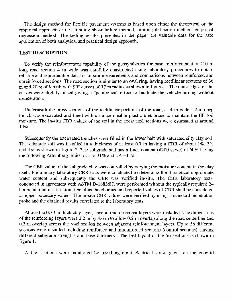
IN-GROUND TEST FOR GEOSYNTHETIC REINFORCED FLEXIBLE PAVED ROADS

ANDREA CANCELLI, UNIVERSITY OF MILAN, ITALY FILIPPO MONTANELLI, TENAX SPA, ITALY

ABSTRACT

The traffic of vehicles on the surface of roads yield deformations in the pavement structure that are a function of both the traveling loads and the mechanical characteristics of the pavement 0 itself. These deformations are either reversible (elastic deflections) or permanent (plastic ruts). With the cyclic application of traffic load, these deformations degrade the pavements and irregularities, ruts, longitudinal asphalt cracks, alligator cracks appear on the surface.

The structural strength of flexible pavement is related to its constitutive elements: the asphalt layer, the granular base, the in-situ subgrade soil and the geosynthetic reinforcement. Geosynthetics are, nowadays, commonly used in flexible road base reinforcement by inserting them typically at the interface between the aggregate base course and the subgrade.

The aim of this in-ground test is to quantify and evaluate the structural contribution of geosynthetic reinforcement to pavement systems and to develop a sound design algorithm based upon actual empirical testing of geogrid reinforced road sections.

INTRODUCTION

This paper deals with the analysis of the results of a full scale pavement test conducted on several reinforced and unreinforced paved sections where the following variables were investigated: subgrade strength, gravel base thickness, geosynthetic type, number of Equivalent Axle Loads (EAL). This is a continuation of previously published papers on the ability of geosynthetics to successfully improve the pavement life and reduce the creation of ruts (Montanelli et. al., 1997 and Cancelli et al. 1996). Similar existing studies were performed on unreinforced and reinforced sections and a comprehensive discussion of the results is given by Perkins and Ismeik (1997).

The design method for flexible pavement systems is based upon either the theoretical or the empirical approaches: i.e.: limiting shear failure method, limiting deflection method, empirical regression method. The testing results presented in the paper are valuable data for the safe application of both analytical and practical design approach.

TEST DESCRIPTION

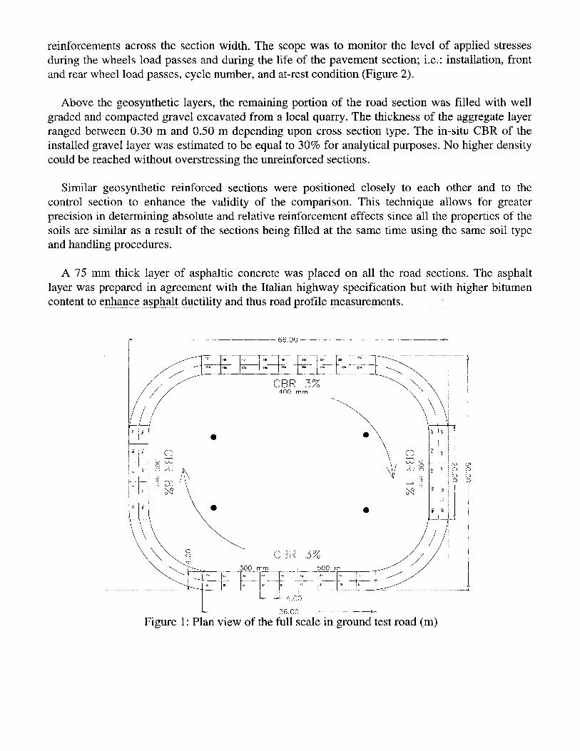
To verify the reinforcement capability of the geosynthetics for base reinforcement, a 210 m long road section 4 m wide was carefully constructed using laboratory procedures to obtain reliable and reproducible data for in-situ measurements and comparisons between reinforced and unreinforced sections. The road section is similar to an oval ring, having rectilinear sections of 36 m and 20 m of length with 90” curves of 17 m radius as shown in figure 1. The outer edges of the curves were slightly raised giving a “parabolica” effect to facilitate the vehicle turning without deceleration.

Underneath the cross sections of the rectilinear portions of the road, a 4 m wide 1.2 m deep trench was excavated and lined with an impermeable plastic membrane to maintain the fill soil moisture. The in-situ CBR values of the soil in the excavated sections were estimated at around 10%.

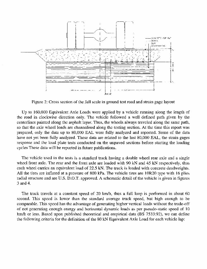
Subsequently the excavated trenches were filled in the lower half with saturated silty clay soil. The subgrade soil was installed in a thickness of at least 0.7 m having a CBR of about l%, 3% and 8% as shown in figure 2. The subgrade soil has a fines content (#200 sieve) of 60% having the following Attemberg limits: L.L. = 3 1% and I.P. = 11%.

The CBR value of the subgrade clay was controlled by varying the moisture content in the clay itself. Preliminary laboratory CBR tests were conducted to determine the theoretical appropriate water content and subsequently the CBR was verified in-situ. The CBR laboratory tests, conducted in agreement with ASTM D-1883:87, were performed without the typically required 24 hours minimum saturation time, thus the obtained and reported values of CBR shall be considered as upper boundary values. The in-situ CBR values were verified by using a standard penetration probe and the obtained results correlated to the laboratory tests.

Above the 0.70 m thick clay layer, several reinforcement layers were installed. The dimensions of the reinforcing layers were 2.2 m by 4.6 m to allow 0.2 m overlap along the road centerline and 0.3 m overlap across the road section between adjacent reinforcement layers. Up to 56 different sections were installed including reinforced and unreinforced sections (control sections), having different subgrade strengths and base thickness’. The test layout of the 56 sections is shown in figure 1.

A few sections were monitored by installing eight electrical strain gages on the geogrid

reinforcements across the section width. The scope was to monitor the level of applied stresses during the wheels load passes and during the life of the pavement section; i.e.: installation, front and rear wheel load passes, cycle number, and at-rest condition (Figure 2).

Above the geosynthetic layers, the remaining portion of the road section was filled with well graded and compacted gravel excavated from a local quarry. The thickness of the aggregate layer ranged between 0.30 m and 0.50 m depending upon cross section type. The in-situ CBR of the installed gravel layer was estimated to be equal to 30% for analytical purposes. No higher density could be reached without overstressing the unreinforced sections.

Similar geosynthetic reinforced sections were positioned closely to each other and to the control section to enhance the validity of the comparison. This technique allows for greater precision in determining absolute and relative reinforcement effects since all the properties of the soils are similar as a result of the sections being filled at the same time using the same soil type and handling procedures.

A 75 mm thick layer of asphaltic concrete was placed on all the road sections. The asphalt layer was prepared in agreement with the Italian highway specification but with higher bitumen content to enhance asphalt ductility and thus road profile measurements. -.............-_-...-.........-....~.--..- _......-...-_..............-.--................-..-.. . ..__.._.._..___..._~....~.~~..~.~~~~~...~..~~.......~.~~~.~....~.~ ..__.._................~~~~.~........~~.-~~...~~......~--~~~.......~~~~~..................~..~......~~..~..~......~~~..........~...

3 66.00

^ _-.-- -- _ .- _____ .-----_ 36.00 .-.- - _-_ .- .- ____. ___._. . _--- 1

Figure 1: Plan view of the full scale in ground test road (m)

T

CONCRETE ASPHALT

Figure 2: Cross section of the full scale in ground test road and strain gage layout

Up to 160,000 Equivalent Axle Loads were applied by a vehicle running along the length of the road in clockwise direction only. The vehicle followed a well defined path given by the centerlines painted along the asphalt layer. Thus, the wheels always traveled along the same path, so that the axle wheel loads are channalised along the testing section. At the time this report was prepared, only the data up to 80,000 EAL were fully analyzed and reported. Some of the data have not yet been fully analyzed. These data are related to the last 80,000 EAL, the strain gages response and the load plate tests conducted on the unpaved sections before starting the loading cycles These data will be reported in future publications.

The vehicle used in the tests is a standard truck having a double wheel rear axle and a single wheel front axle. The rear and the front axle are loaded with 90 kN and 45 kN respectively, thus each wheel carries an equivalent load of 22.5 kN. The truck is loaded with concrete deadweights. All the tires are inflated at a pressure of 800 kPa. The vehicle tires are lOR20 type with 16 plies radial structure and are U.S. D.O.T. approved. A schematic detail of the vehicle is given in figures 3 and 4.

The truck travels at a constant speed of 20 km/h, thus a full loop is performed in about 60 second. This speed is lower than the standard average truck speed, but high enough to be comparable. This speed has the advantage of generating higher vertical loads without the trade-off of not generating enough energy and horizontal dynamic loads as per pseudo-static speed of 10 km/h or less. Based upon published theoretical and empirical data (BS 7533:92), we can define the following criteria for the definition of the 80 kN Equivalent Axle Load for each vehicle lap:

9.0 t, dual wheel axle loa

Pirelli TH 20 Radial 16 PLIES lO.OOR20 DOT XJ 2J APPROVED

Figure 3: Side view of the truck vehicle and longitudinal cross section

a SI I

0 z 1 -- -.

5 3

7

L---- ---. --~-------~.-4 o()(+-------- ---A

I ,200~12001 1200 --,-?I% REAR AXLE I

125 125

L fz, 1850 ._ - ----mu!!., F-R[-JNl- AXL_ E

Figure 4: Rear view of the truck vehicle and cross section

l The rear double wheel axle load of 90 kN is equivalent to 1.61 EAL of 80 kN (18,000 lb.) due to the fourth power law applied to the load ratio: (90/80)4 = (factor of 1.61);

l The front single wheel axle load of 45 kN is equivalent, for road sections having a structural number SN between 2.5 and 4.0, to a double wheel axle load of 90’kN (factor of 1.61);

l Each axle passes, being channalised along a single track and not distributed across the full width of the road is equivalent to 3 passes (factor of 3) (Figure 5,6 and 7);

l Thus, for each vehicle cycle, the EAL load factor is: (1.61 + 1.61) x 3 = 9.66. For simplicity, we will use a factor of 10 in the following discussions.

Some of the geosynthetics tested are listed in table 1 together with their reported properties. The products tested can be classified among the following categories:

a) single layer biaxially oriented polypropylene geogrids manufactured by extrusion process; b) multi-layers biaxially oriented polypropylene geogrids manufactured by extrusion process; c) woven polyester geogrids; d) slit film woven fabrics; e) composite structures: i.e.: extruded eeoerid and nonwoven geotextiles. woven and nonwoven

/

geotextiles. I w u U

Table 1: Product codes and nominal properties

Product Category MDxTD MDxTD MDxTD MDxTD Code Tensile Strength, Tensile Strength Junction Strength, Aperture Size,

N. Layers kN/m @ 2% E, kNm kN/m mm GGML2 b - 2 13.5 X 20.5 4.1 X 6.0 12.2 x 18.5 21 X25 GGML3 b - 3 20.0 x 30.7 6.1 X 9.0 18.0 X 27.7 14x 17 GGMLS b - 5 22.0 x 35.0 6.0 X 10.0 19.8 x 31.5 12x 12 GGRl a-l 12.1 X 20.5 4.0 X 5.8 10.9 x 18.4 25 X 33 GGR2 a- 1 17.0 x 31.5 5.4 x 8.7 15.3 X 28.3 25 X 33 WGTX- d- 1 30.0 x 30.0 4.0 x 5.0 I-- --I

DATA COLLECTION AND ANALYSIS

The rut depths were measured as a function of the numbers of cycles, aggregate thickness, sub- grade shear strength and geosynthetic type. The data were collected to determine the ability of the reinforcements to distribute the load over a wider sub-grade surface area, to minimize differential settlement and thus to extend the pavement life.

The rut depths were measured by means of a specially designed rectilinear beam, having a 2 m span, over which an electronic micrometer having an accuracy of 20.01 mm was installed. The beam was placed across the road section to be measured and properly positioned horizontally by

means of a waterlevel having an accuracy of +0.02 mm/m; thus an overall accuracy of +0.05 mm across the beam width for the overall device was reached (figure 8).

The test sections were marked with a solid yellow line along the centerline and along the measurement cross-sections placed in the middle of each section. The transversal borderlines of each section were marked with dotted yellow lines (figure 9). The measurement cross-section lines were marked with a Fisher type nail at the intersections with the centerline.

The head of the nails were used during each measurement either for shooting the elevation measurements by means of a telescopic unit and for zeroing the micrometer prior to taking the measurements. The rut measurements across the cross-sections were taken every 0.10 m starting from the nail head.

The rut depths were measured at 0, 30, 50, 100, 300, 500, 1000, 2000, 4000, 8000 cycles on most of the sections, together with the elevation quotes. In the following analysis, the maximum rut depths for each cross-section is defined as the difference of the maximum uplift and downlift values for the specific cycle of measures (figure 11). This criterion is given by the fact that, for the quality of the road surface, both the truck and the driver are sensible to the difference 8 between the uplift and the downlift rut and not to the downlift values only. .

Post traffic photos on most of the sections were taken to record and qualitatively compare the performance behavior. The asphalt layer was inspected to determine the longitudinal and transverse cracks or the formation of alligator cracks.

Some measurements and tests were performed prior to the actual experimental portion of the full scale test. The soil and asphalt were classified in respect to the type, gradation and moisture content, and CBR tests were performed both in the laboratory and in-situ In situ the layer thickness and density were inspected. On the geosynthetics, the following tests were performed: tensile properties, unit weight, mesh size and other typical QC tests. Load plate tests were conducted on the unpaved sections for the determination of the Ev2 moduli performed in agreement with SNV 670317a with 300 mm plate. In addition up to 8 strain gages were glued on the geogrid layers for the determination of actual in-situ geogrid stress (Figure 2). 8

SCOPE OF THE TEST ANALYSIS

The results of the reinforced sections are compared with the corresponding unreinforced section to show the advantages of geosynthetics in increasing the road service life, reducing the rut depth and savings in aggregate. The tests are analyzed to show the following results: l comparisons between reinforced and unreinforced sections; l comparisons between reinforced sections at several gravel thickness’; l comparisons between reinforced sections at different CBRs; l qualitative comparison between geosynthetics.

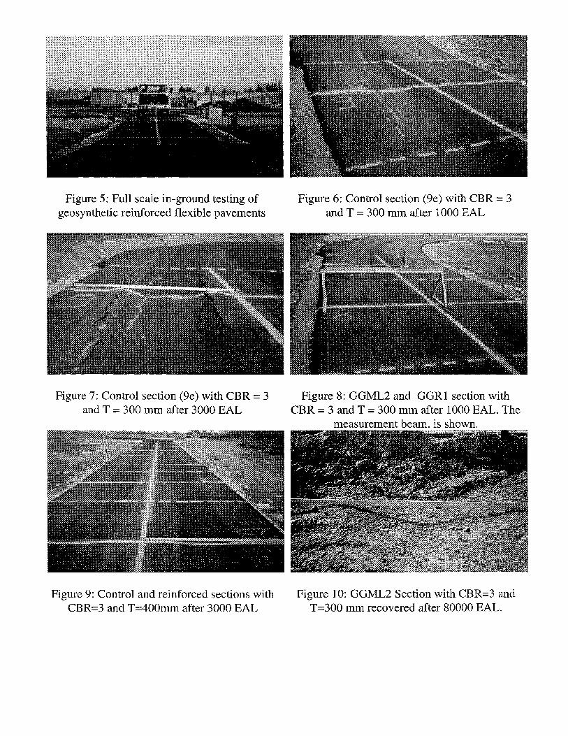
Figure 5: Full scale in-ground testing of Figure 6: Control section (9e) with CBR = 3 geosynthetic reinforced flexible pavements and T = 300 mm after 1000 EAL

Figure 7: Control section (9e) with CBR = 3 and T = 300 mm after 3000 EAL

Figure 8: GGML2 and GGRl section with CBR = 3 and T = 300 mm after 1000 EAL. The

measurement beam. is shown.

Figure 9: Control and reinforced sections with CBR=3 and T=400mm after 3000 EAL

Figure 10: GGML2 Section with CBR=3 and T=300 mm recovered after 80000 EAL.

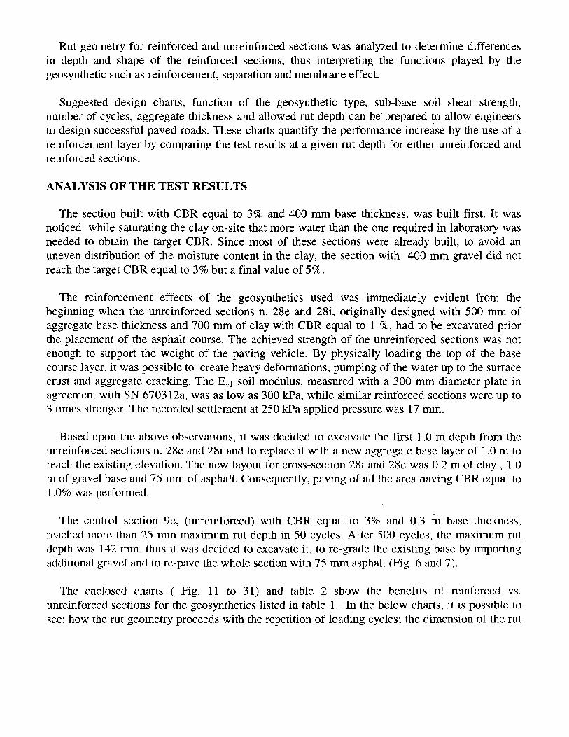
Rut geometry for reinforced and unreinforced sections was analyzed to determine differences in depth and shape of the reinforced sections, thus interpreting the functions played by the geosynthetic such as reinforcement, separation and membrane effect.

Suggested design charts, function of the geosynthetic type, sub-base soil shear strength, number of cycles, aggregate thickness and allowed rut depth can be’ prepared to allow engineers to design successful paved roads. These charts quantify the performance increase by the use of a reinforcement layer by comparing the test results at a given rut depth for either unreinforced and reinforced sections.

ANALYSIS OF THE TEST RESULTS

The section built with CBR equal to 3% and 400 mm base thickness, was built first. It was noticed while saturating the clay on-site that more water than the one required in laboratory was needed to obtain the target CBR. Since most of these sections were already built, to avoid an uneven distribution of the moisture content in the clay, the section with 400 mm gravel did not reach the target CBR equal to 3% but a final value of 5%.

The reinforcement effects of the geosynthetics used was immediately evident from the beginning when the unreinforced sections n. 28e and 28i, originally designed with 500 mm of aggregate base thickness and 700 mm of clay with CBR equal to 1 %, had to be excavated prior the placement of the asphalt course. The achieved strength of the unreinforced sections was not enough to support the weight of the paving vehicle. By physically loading the top of the base course layer, it was possible to create heavy deformations, pumping of the water up to the surface crust and aggregate cracking. The EV1 soil modulus, measured with a 300 mm diameter plate in agreement with SN 6703 12a, was as low as 300 kPa, while similar reinforced sections were up to 3 times stronger. The recorded settlement at 250 kPa applied pressure was 17 mm.

Based upon the above observations, it was decided to excavate the first 1.0 m depth from the unreinforced sections n. 28e and 28i and to replace it with a new aggregate base layer of 1.0 m to reach the existing elevation. The new layout for cross-section 28i and 28e was 0.2 m of clay , 1.0 m of gravel base and 75 mm of asphalt. Consequently, paving of all the area having CBR equal to 1 .O% was performed.

The control section 9e, (unreinforced) with CBR equal to 3% and 0.3 m base thickness, reached more than 25 mm maximum rut depth in 50 cycles. After 500 cycles, the maximum rut depth was 142 mm, thus it was decided to excavate it, to re-grade the existing base by importing additional gravel and to re-pave the whole section with 75 mm asphalt (Fig. 6 and 7).

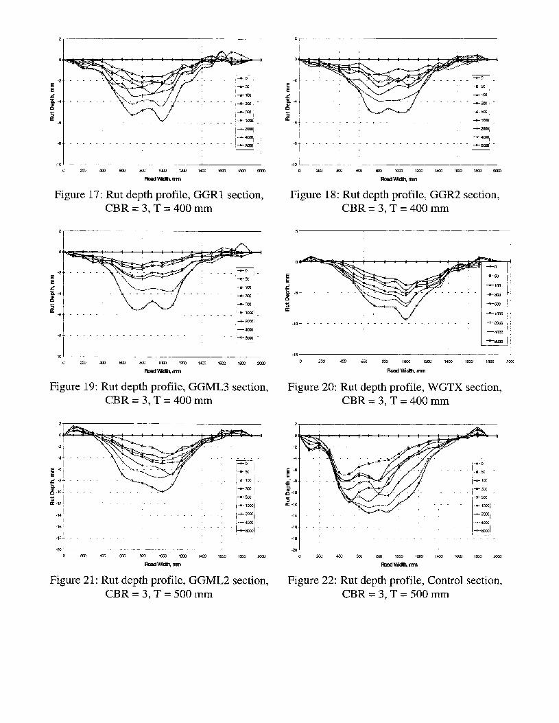
The enclosed charts ( Fig. 11 to 31) and table 2 show the benefits of reinforced vs. unreinforced sections for the geosynthetics listed in table 1. In the below charts, it is possible to see: how the rut geometry proceeds with the repetition of loading cycles; the dimension of the rut

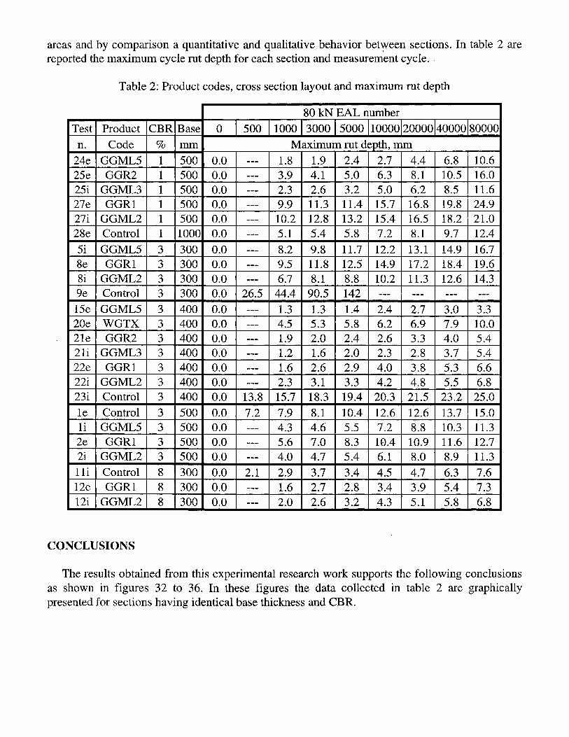
areas and by comparison a quantitative and qualitative behavior between sections. In table 2 are 6 reported the maximum cycle rut depth for each section and measurement cycle. .

Table 2: Product codes, cross s action layout and m; .ximum rut depth

80kNEALr umber 500 1000 I 3000 I5000 Test Product CBR Base 0

n. Code % mm Maximum rut d zpth;mm 1.8 ( 1.9 I 2.4 2.7 1 4.4 1 6.8 1 10.6 24e [GGML51 1 1 500 1 0.0 -me

25e 1 GGR2 1 1 I500 1 0.0 25 I GGML3 I 1 I 500 I 0.0 27e 1 GGRl I 1 I500 I 0.0 2% 1 GGML2 I 1 1500 1 0.0 28e I Control I 1 IlOOOl 0.0 5i I GGMLS I 3 I 300 1 0.0 8e GGRl 3 300 0.0 8i GGML2 3 300 0.0 9e I Control I 3 I 300 1 0.0 15e 1 GGML5 I 3 I 400 1 6.0 20e WGTX 3 400 0.0 21e GGR2 3 400 0.0 21i I GGML3 I 3 1400 1 0.0

3.9 I 4.1 I 5.0 6.3 1 8.1 1 10.5 1 16.0 5.0 1 6.2 1 8.5 1 11.6 15.7 16.8 [ 19.8 1 24.9 15.4 1 16.5 1 18.2 1 21.0

I--

2.3 1 2.6 1 3.2 9.9 I 11.3 I 11.4 10.2 1 12.8 1 13.2 5.1 1 5.4 1 5.8 7.2 1 8.1 1 9.7 1 12.4

12.2 1 13.1 1 14.9 1 16.7

---

8.2 1 9.8 1 11.7 9.5 1 11.8 1 12.5 14.9 1 17.2 1 18.4 1 19.6

10.2 1 11.3 I 12.6 I 14.3 B-M

6.7 1 8.1 1 8.8 26.5 44.4 1 90.5 1 142

1.3 11.3 r 174 2.4 12.7-3.07- 3.3 45 . 5.3 1 5.8 6.2 1 6.9 1 7.9 1 10.0 19 . 2.0 1 2.4 26 . 33 . 1)1)-

111

-mm

-111

13.8 72 l

1 1 1

m-m

--I

21 . --I -II-

1.6 1 2.0 23 . 28 . 16 . 2.6 1 2.9 38 . 22e GGRl 3 400 0.0

22i GGML2 3 400 0.0 23i Control

23 . 42 . 48 . 18.3 1 19.4 21.5 23.2 1 25.0

le I Control I 3 I 500 I 0.0 li 1 GGMLS 1 3 I500 1 0.0 2e GGRl 3 500 0.0 2i GGML2 3 500 0.0 lli I Control 1 8 1 30m 12e 1 GGRl I 8 1300 I 0.0 12i ( GGML2 I 8 I 300 I 0.0

8.1 r10.4 12.6 12.6 4.6 1 5.5 72 .

56 . 7.0 1 8.3 11.6 1 12.7 61 . 80 . 8.9 1 11.3

29 . 6.3 1 7.6 16 . 2.7 1 2.8 34 . 39 . 5.4 I 7.3 20 . 2.6 1 3.2 43 . 51 . 5.8 1 6.8

CONCLUSIONS

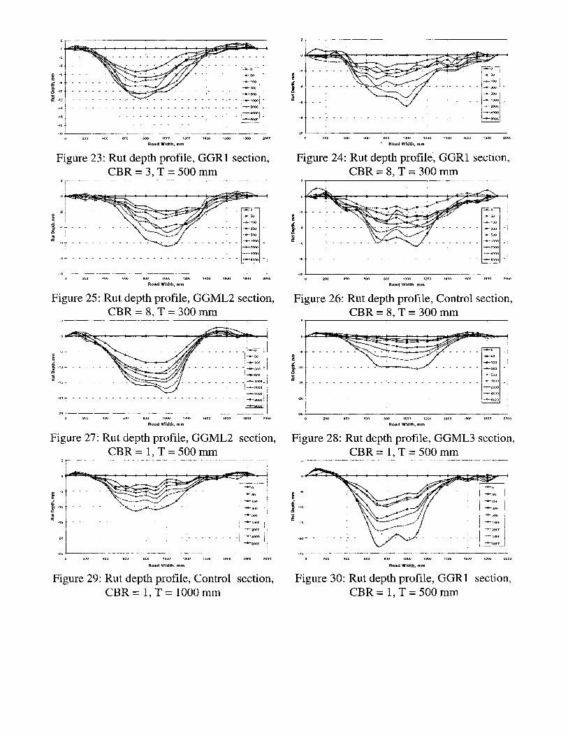
The results obtained from this experimental research work supports the following conclusions as shown in figures 32 to 36. In these figures the data collected in table 2 are graphically presented for sections having identical base thickness and CBR.

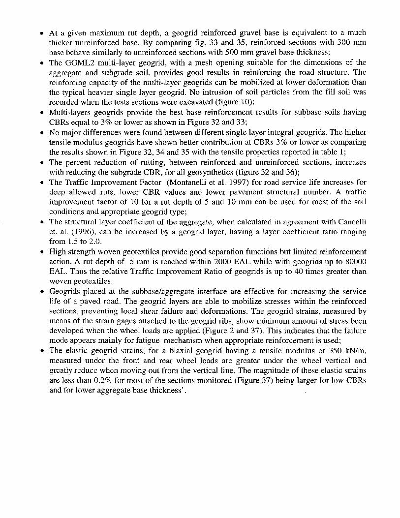
l At a given maximum rut depth, a geogrid reinforced gravel base is equivalent to a much thicker unreinforced base. By comparing fig. 33 and 35, reinforced sections with 300 mm base behave similarly to unreinforced sections with 500 mm gravel base thickness;

l The GGML2 multi-layer geogrid, with a mesh opening suitable for the dimensions of the aggregate and subgrade soil, provides good results in reinforcing the road structure. The reinforcing capacity of the multi-layer geogrids can be mobilized at lower deformation than the typical heavier single layer geogrid. No intrusion of soil particles from the fill soil was recorded when the tests sections were excavated (figure 10);

l Multi-layers geogrids provide the best base reinforcement results for subbase soils having CBRs equal to 3% or lower as shown in Figure 32 and 33;

.

l No major differences were found between different single layer integral geogrids. The higher tensile modulus geogrids have shown better contribution at CBRs 3% or lower as comparing the results shown in Figure 32, 34 and 35 with the tensile properties reported in table 1;

l The percent reduction of rutting, between reinforced and unreinforced sections, increases with reducing the subgrade CBR, for all geosynthetics (figure 32 and 36);

l The Traffic Improvement Factor (Montanelli et al. 1997) for road service life increases for deep allowed ruts, lower CBR values and lower pavement structural number. A traffic improvement factor of 10 for a rut depth of 5 and 10 mm can be used for most of the soil conditions and appropriate geogrid type;

l The structural layer coefficient of the aggregate, when calculated in agreement with Cancelli et. al. (1996), can be increased by a geogrid layer, having a layer coefficient ratio ranging from 1.5 to 2.0.

l High strength woven geotextiles provide good separation functions but limited reinforcement action. A rut depth of 5 mm is reached within 2000 EAL while with geogrids up to 80000 EAL. Thus the relative Traffic Improvement Ratio of geogrids is up to 40 times greater than woven geotextiles.

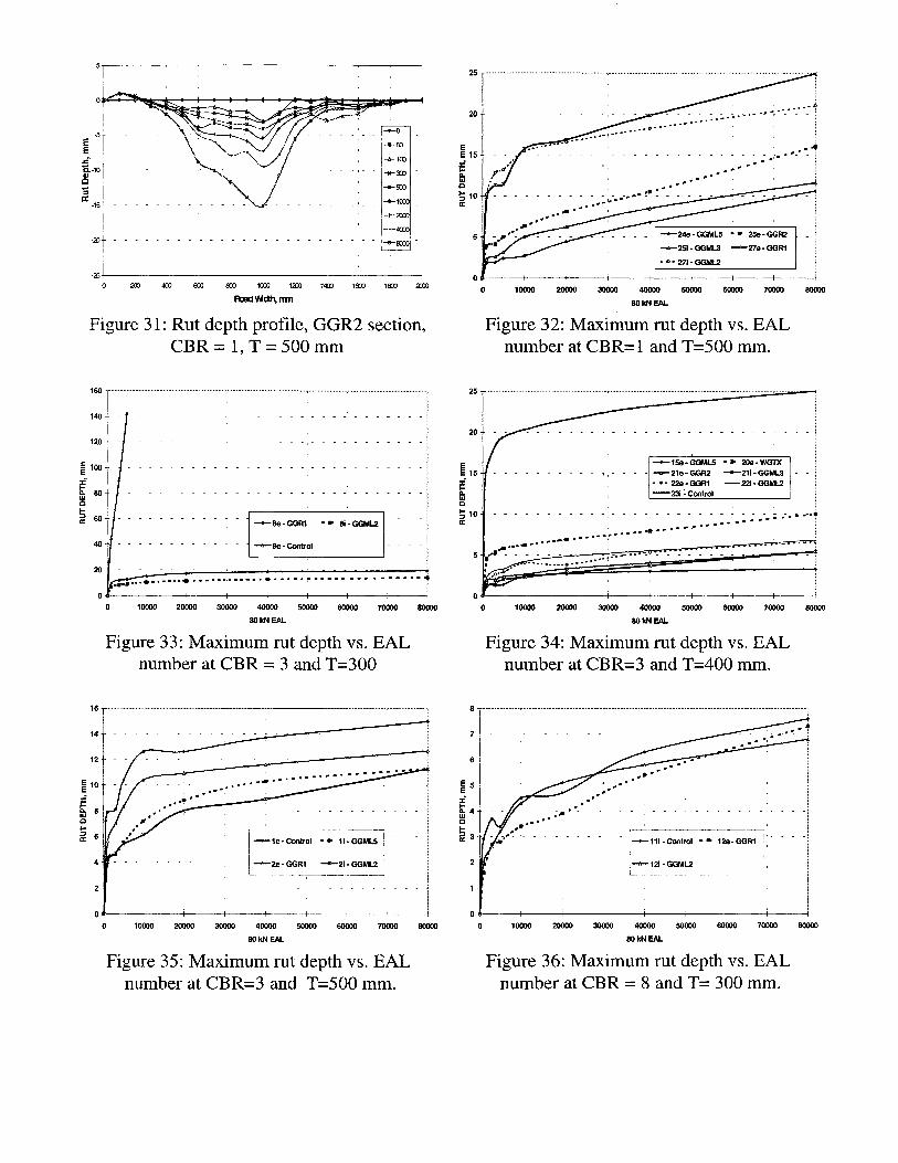
l Geogrids placed at the subbase/aggregate interface are effective for increasing the service life of a paved road. The geogrid layers are able to mobilize stresses within the reinforced sections, preventing local shear failure and deformations. The geogrid strains, measured by means of the strain gages attached to the geogrid ribs, show minimum amount of stress been developed when the wheel loads are applied (Figure 2 and 37). This indicates that the failure mode appears mainly for fatigue mechanism when appropriate reinforcement is used;

l The elastic geogrid strains, for a biaxial geogrid having a tensile modulus of 350 kN/m, measured under the front and rear wheel loads are greater under the wheel vertical and greatly reduce when moving out from the vertical line. The magnitude of these elastic strains are less than 0.2% for most of the sections monitored (Figure 37) being larger for low CBRs and for lower aggregate base thickness’.

,

-100 1 /

0 200 400 600 a00 loo0 12aI 1400 1600 la00 xxx)

Roadwidth,m

Figure 12: Rut depth profile, Control section, CBR=3,T=3OOmm

Figure 11: Cross-sectional profile of the test sections, showing the maximum (total) rut depth

and downlift and uplift rut.

- - - -

-tO

.Ja..w -

--bloO

-n-300 -

-E-500

-+-1ocxJ -

+2om

-4000

-8000

-+O

..a.. i=JJ

-&-loo -

*3CO -

-X-500

+1mo-

+2ooo-

-4000

-wcoo-

s CT -12

-14 J -20 0 200

Figure 14: Rut depth profile, GGRl section, CBR=3,T=3OOmm

Figure 13: Rut depth profile, GGML2 section, CBR=3,T=300mm

2 I 2-

-24 - - - _ t

v ._-,

-+0

..*-. 5(J

--leloo

*ZOO

+500

+1000

+2000

-4000

-8000 __.- _.. - ? - -

+0 ---I- ..(p-. CJ)

--blOO

*m -

-?K-500

l-

+1coo /

+2000

--4om

+8ooo- -8. - I .- -10 I--- __------- - . . .._ - -.-.- --..- I .--_ -L--. ._-----._---_/__L 2&j I- --__-. .

0 200 400 600 mo loo0 1200 1400 1600 1800 2ca

Fioi3dwdth,m

0 200 400 600 800 Km 1200 1400 1600 leo0 2cm

l3oad\Mdth,m

Figure 15: Rut depth profile, Control section, Figure 16: Rut depth profile, GGML2 section, CBR=3.T=400mm CBR=3,T=400mm

I

-+-* -

-ii+-!3

-a-100

*300 -

-u-500

-1oco

+2OW

--4ooo

-c*-aooo-

d 5 a s a

1”

0 200 400 600 600 loo0 1200 1400 1600 1800 m

ludwclth,ITm

Figure 18: Rut depth profile, GGR2 section, CBR=3,T=400mm

0 200 403 600 tm loo0 1200 1400 1600 laoo 2ooo

RoadMdth,m

Figure 17: Rut depth profile, GGRl section, CBR=3,T=400mm

21 I

+0

-+-60

-a-loo

*3CO

-!%Cl

-1000

+2ooo

-4000

-8ooo

-* -

..a.. !jo

*100

*m -

-w-500

+loo0

+2000

-4WO

-s-8000-

---- -- - ------_-__

-1-J

0 200 400 600 800 loo0 1200 1400 1600 1800 2ooc

Roadwidth,m

Figure 19: Rut depth profile, GGML3 section, Figure 20: Rut depth profile, WGTX section, CBR=3,T=400mm CBR=&T=400mm

-CO

-P- 50

+100 -

*300 . ..*e. 500

-+-looo -

+2ooo.. ..a- 4(-j@j

+acm- -7

-14-- - - - - -

-16-7 _ _ - - -_-- ______

1400 1600 la00 2ao

&----.--~-- ---_ - ---’ -----L--- - --__ ____.______________~

0 2m 400 600 8cQ lcxn Km 1400 1600 lam 2oco

FloEwnActtr,IYm

Figure 21: Rut depth profile, GGML2 section, Figure 22: Rut depth profile, Control section, CBR=3,T=5OOmm CBR=3,T=5OOmm

-6

I -20 J , 0 200 400 600 800 1000 1200 1400 1600 1000 2000

Road Width, mm

-10

0 200 400 600 800 1000 1200 1400 1600 1600 2000

8 Road Width, mm

Figure 23: Rut depth profile, GGRl section, CBR=3,T=500mm

Figure 24: Rut depth profile, GGRl section, CBR=8,T=3OOmm

2 2 1 I

0

.

Ii

-4

-6

- - r - - - - - - - - , - - - I - -

- - r - - ,- - - - - - - - -

- - - - - - - - - - - - - ___-______

--- - - --- --- - - - - _-________ -6

-10 J 0 200 400 600 600 1000 1200

Road Width, mm

J 1400 1600 1600 2000 200 800 1000 1200

Road Width, mm

2000

Figure 25: Rut depth profile, GGML2 section, Figure 26: Rut depth profile, Control section, CBR=8,T=300mm CBR=8,T=3OOmm 5 5

--to

.*-* 50

+100

*300 -

-500 I -1000

+2000

-4000

i -8000 -

f B if .,o - - - - - ,- - - - 2 -15 _ _ _ _ - - - - I_ - - - - - - - - - -

200 400 600 000 1000 1200

Road Width, mm 1400 1600 1000 2000 800 1000 1200

Road Width, mm

Figure 27: Rut depth profile, GGML2 section, Figure 28: Rut depth profile, GGML3 section, CBR=l,T=500mm CBR=l,T=5OOmm

i -5

. g -10

s a -15

--.- -_ 1800 2000 800 1000 1200

Road Width, mm

600 1200 1400 1600 400 600 800

Road Width, mm

Figure 29: Rut depth profile, Control section, Figure 30: Rut depth profile, GGRl section, CBR = 1, T = 1000 mm CBR= l,T=5OOmm

5

0

-5

E

c" E-10

8

s K

-15

-a

-25

---- - --- - - --- - - -- -_______

-+O

-4-50

-bloo

*300 -

*SOJ

-+lOCO

+ZWO

-4coo

+m-

0 2x3 400 600 800 mtl mo 1400 lalo la00 mo

F+3tWM~mn

Figure 31: Rut depth profile, GGR2 section, Figure 32: Maximum rut depth vs. EAL CBR= l,T=SOOmm number at CBR=l and T=500 mm.

160

140

120

p0 .

z 4 80 P k 2 60

40

20

0

-_-____---_--- ---__-_____

i ------_---_--- - -----_____ I

-&-GGRI -) 8i-GGML2 : - - -

-_-__-______ 1 -9e-controi

80kNEAL

Figure 33: Maximum rut depth vs. EAL Figure 34: Maximum rut depth vs. EAL number at CBR = 3 and T=300 number at CBR=3 and T=400 mm.

16

0 10000 20000 30000 40000 50000 60000 70000 80000 0 10000 20000 30000, 40000 50000 60000 70000 80000

80kNEAL 80kNEAL

Figure 35: Maximum rut depth vs. EAL Figure 36: Maximum rut depth vs. EAL number at CBR=3 and T=500 mm. number at CBR = 8 and T= 300 mm.

25

E E I5

f ti P

g IO K

25

20

E I5 m E

8 2 IO K

5

0

. . . . . . ..‘..“.........................................................~...........-........... . . . . . . . . . . . . . . ..“................................................

- - - I- - - -I-

- - - - - ____-______-_

0 10000 20000 30000 40000 50000 60000 70000 80000

80kNEAL

0 10000 20000 30000 40000 50000 60000 7OWO 80000

80kNEAL

8 . . . . . . . . . . . . . . . . . . . . . . . . . . . . . . . . . . . . . . . . . . . “ . . . . . . . . . . . . . . . . . . . . . . . . . . . . . . . . . . . . . - . . . . . . . . . . . . . . . . . . . . . . . . . . . . . . . . . . . . . . . . . . - . . . . . . . . . . . . . . . . . . . . . . . . . . . . . . . . . , . _ . . . . _ . . . . . _ . . . _ _ _ . .

6

--____ - -.-.______ +IIi-Control I) 12e-GGRI '-

-a-121-GGML2 l- -.-____-__---~~ -...-.

0.08

0.04

0.02

0.00

Geogrid Strain under Axle Loads BIAXIAL GEOGRID @ 8000 cycles, CBR=3% AND 300 mm BASE

+Oa

+l b . . .:.:,: .._ ,., 2 c

++ 3d

+4e

-e-5%

10 . 15 . 2.0 2.5

Time, (set)

Figure 37: Geogrid rib tensile strain at 8000 cycles measured under the front (left) and rear (right) wheel passage.

REFERENCES

ASTM D1883:87, 1987, “Standard Test Method for CBR (California Bearing Ratio) of Laboratory- Compacted Soils” Annual Book of ASTM Standards.

BS 7533:1992, 1992, “Guide for structural design of pavements constructed with clay of concrete block pavers” British Standards Institution.

Cancelli, A., Montanelli, F., Rimoldi, P., and Zhao, A., 1996, “Full scale laboratory Testing on geosynthetics reinforced paved roads” Proceedings of the International Symposium on Earth Reinforcement, pp. 573-578. .

Montanelli, F., Zhao, A., and Rimoldi, P., i 997, “Geosynthetics-reinforced pavement system: testing and design” Proceeding of Geosvnthetics ‘97, pp. 619-632.

Perkins, S.W., and Ismeik, M., 1997, “A synthesis and evaluation of geosynthetic-reinforced base layers in flexible pavements: part I”, Geosvnthetics International, pp. 549-604.

SNV 6703la, 1981, “Essai de charge avec plaques M $ Association Suisse de Normalisation.