Embed Size (px)
Citation preview
Author:
J. Kars, University of Twente
Master: Industrial Engineering & Management
Track: Production & Logistics Management
Supervisors:
Dr. ir. J.M.J. Schutten, University of Twente
Dr. P.C. Schuur, University of Twente
Ing. E. Mulder, DS Smith Packaging B.V.
Improved performance by integrated
corrugator and convertor scheduling
Master thesis, September 2014

Author
J. (Jeroen) Kars
University
Unversity of Twente
Master programme
Industrial Engineering & Management
Specialization
Production & Logistics Management
Graduation date
19 September 2014
Graduation committee
Dr. ir. J.M.J. Schutten
University of Twente
Dr. P.C. Schuur
University of Twente
Ing. E. Mulder
DS Smith Packaging B.V.
University of Twente
Drienerlolaan 5
7522 NB Enschede
The Netherlands
DS Smith Packaging B.V.
Coldenhovenseweg 130
6961 EH Eerbeek
The Netherlands

DS Smith Packaging B.V. Management Summary i
MANAGEMENT SUMMARY This research is as part of the Master Industrial Engineering and Management at the University
of Twente. The aim of this project is to deliver a solution that models the tasks of the production
planners at DS Smith Packaging B.V. located in Eerbeek, The Netherlands. This model gives
valuable insights for improving production planning and scheduling. This solution decreases the
tardiness of orders from to 7.04% and even to 2.76% if we correct for orders that are confidential
only 4 hours tardy.
PROBLEM IDENTIFICATION Currently DS Smith is using an ERP system that separately solves the cutting stock problem and
scheduling problems. Production planners build and change production schedules based on
intuition and experience. However, the complexity is high, so it is hard to keep track of the
performance of a schedule while making the schedules separately. This results in schedules that
cause disruptions in the production process. We use the following main research question for
this research:
“How should DS Smith Packaging B.V. solve the cutting stock problem and generate
production schedules in order to find a good balance between minimizing waste,
minimizing idle times of machines, and maximizing the on time delivery performance of
orders?”
THE GENERAL MODEL In order to model the different tasks of the production planners, we use a modular approach.
Each module performs a task of the production planners. We have to deal with NP-hard
problems. Therefore we decide that we are modeling the different tasks in modules that solve
the problems separately instead of solving the whole problem at once. The solution consists of
five modules: an order selection module, a cutting stock problem module, a corrugator
scheduling module, a converting scheduling module, and a Pentek (buffer zone) module.
The order selection module selects the orders that enter the cutting stock problem module.
Deckle solutions are generated in the cutting stock problem module. A deckle solution is the set
of Corrugator Instruction (CI) jobs of a certain board grade. These deckle solutions are
scheduled in the corrugator scheduling module with the objective to minimize setups of the
corrugator machine and tardiness of the corrugator jobs. The converting scheduling module
schedules the converting jobs based on the FIFO principle by using the first available production
time. After that, a load balancing procedure is used to check if alternative machine routings may
improve the solution. The Pentek module uses the starting and finishing times of the corrugator
and converting jobs to calculate the fill rate of the Pentek. This module may be used for timely
identifying problems caused by the Pentek and make important (re)scheduling decisions.
ALTERNATIVES We formulate alternative objective functions for solving the cutting stock problem. Currently,
trim loss minimization is used as objective function. We formulate objective functions that
minimize the needed total run length of the corrugator machine and an alternative that
minimizes production costs of the corrugator machine. For solving the corrugator scheduling
problem we formulate three alternative approaches. The first approach uses a 1-Opt heuristic.
This heuristic selects a random deckle solution and inserts it at another place. The second is a

DS Smith Packaging B.V. Management Summary ii
heuristic based on simulating annealing (SA) and the third heuristic is based on the adaptive
search (AS). After each approach, we use an integrated corrugator and converting scheduling
heuristic. We also formulated an alternative where we only use the integrated heuristic. This
results in eight alternative solutions that we test with a simulation for weeks 14 and 15 in 2014.
RESULTS The alternative minimum run length and minimum cost objective function show significant
differences on total run length, trim loss, and number of paper width changes with the trim loss
objective function. We propose the cost objective function with production costs of per confidential
hour as best solution. Even if the production cost per hour ranges between €600 and €1600, the
maximum cost deviation is at most 0.07%.
We evaluate the eight model alternatives based on eight criteria: tardiness, earliness, output of
the corrugator machine, trim loss, waiting time, waiting on corrugator (WOC) idle time, fill rate
of the Pentek, and simplicity of the alternative (see Table 0.1 for the overview of the evaluation).
We propose alternative 5 as best solution. This alternative uses the 1-Opt heuristic and the cost
objective for the cutting stock problem. It performs best on tardiness (2.76% corrected tardy
orders). This is a large improvement compared to the current situation where of the confidential
orders are tardy. Next to this, it also performs well on the output of the corrugator, WOC idle
time, fill rate of the Pentek, and on simplicity. Alternatives 3, 4, 7, and 8 are not interesting
because they score low on tardiness, earliness, output of the corrugator machine, or fill rate of
the Pentek.
Alternative Tardiness Earliness Output Trim loss Waiting
time WOC
idle time Fill rate Simplicity
1 (1-Opt – trim) + +/- +/- - +/- + +/- +
2 (SA – trim) ++ +/- +/- - +/- +/- +/- -
3 (AS – trim) -- - +/- - +/- +/- -- -
4 (Int – trim) +/- + - - + - - +
5 (1-Opt – cost) ++ +/- + - - + + + 6 (SA – cost) + +/- +/- - +/- +/- + -
7 (AS – cost) -- - + - - + -- -
8 (Int – cost) +/- + - - + - +/- + Table 0.1 Final results: the trim loss results of all alternatives are worse than the current situation and
comparable to each other. Therefore, all get the score -. In bold the alternative we propose.
CONCLUSIONS The Pentek module gives a good insight in the future fill rate of the Pentek and helps in making
timely (re)scheduling decisions. Moreover, we recommend implementing the cost minimization
objective for the cutting stock problem. Another important recommendation is the use of
performance measurements for scheduling. Currently the production planners do not have
insight in the performance of the generated schedules. Finally, implementing the method for
coping with uncertainty improves the robustness and reliability of production scheduling.
Overall, this research has provided valuable insights that help DS Smith in improving their
production planning and scheduling. This may lead to a decrease in waste and idle time of
machines, and an increase in the on time delivery performance. This helps DS Smith in being
more competitive in the market and to meet customer demands.
DS Smith Packaging B.V. Preface iii
PREFACE This thesis is the result of my graduation project at DS Smith Packaging B.V., located in Eerbeek.
The aim of this project was to deliver a solution that models the different tasks of the production
planners. This was a very challenging goal; the situation at DS Smith is complex with many
restrictions and limitations that need to be considered. I am happy that after seven months I
completed the project with the expected result.
I thank DS Smith for giving me the opportunity to perform this graduation project. I really enjoyed
my time in Eerbeek and learned a lot during the project about business specific processes and
working in a professional environment. I thank my colleagues Evert Berends and Riny Wiggers for
their help with understanding the whole planning and scheduling process. I also thank Edwin
Mulder, my external supervisor, for his support during the project. Next to them, I thank Marco
Schutten and Peter Schuur, my supervisors from the University of Twente, for giving me valuable
feedback for writing this thesis. This thesis would have been of less quality without their feedback.
Finally, I thank my family and friends for their unconditional support during my study and
graduation. Their support, encouragement, and belief have been of great help for successfully
ending my study.
Jeroen Kars
Eerbeek, September 2014

DS Smith Packaging B.V. Preface iv

DS Smith Packaging B.V. Glossary and list of abbreviations v
GLOSSARY AND LIST OF ABBREVIATIONS AS: Adaptive Search, construction algorithm for solving combinatorial optimization problems
Board grade: The paper quality measured in grams per square meter
CI job: Corrugator Instruction job
Converting machines: The machines that convert the corrugated board sheets into boxes
Corrugating Instruction (CI) job: A corrugator job consisting of one or two orders of a certain board grade for a certain run length
Corrugator machine: The machine that makes the corrugated board sheets
Corrugator roll: Part of the corrugator machine that makes the flutes of the cardboard
Creases: A line made on the corrugated board to ease folding
CSP: Cutting stock problem
Die Cutter: Converting machine that has a high die cutting capability and no ability to fold boxes
Deckle solution (ds): Combination of jobs for the corrugator machine in order to reduce waste
Flute: The wavy paper in the middle of corrugated board
FFG: Flexo Folder Gluer, a converting machine with a small die cutting capability and the ability to fold boxes
1-Opt: Greedy Insertion heuristic
IF: In Full delivery, order is delivered between the minimum and maximum order size
ILP: Integer Linear Programming
MILP: Mixed Integer Linear Programming
OT: On Time delivery of an order
OTIF: On Time and In Full delivery of an order
Pentek: This is the automated WIP buffer between the corrugator machine and the converting machines
RCCP: Rough Cut Capacity Planning
SA: Simulated Annealing, local search algorithm for solving combinatorial optimization problems
Trim loss: Waste of the corrugator machine at the sides
TS: Tabu Search, local search algorithm for solving combinatorial optimization problems
WIP: Work in Process
WOC: Waiting on Corrugator
WOP: Waiting On Pentek

TABLE OF CONTENTS
Management Summary ................................................................................................................. i
Preface ....................................................................................................................................... iii
Glossary and list of abbreviations ................................................................................................. v
1. Introduction ......................................................................................................................... 1
1.1. COMPANY DESCRIPTION ................................................................................................................ 1
1.2. PROBLEM DESCRIPTION ................................................................................................................ 2
1.3. RESEARCH QUESTIONS ................................................................................................................. 3
2. Current situation .................................................................................................................. 5
2.1. THE GENERAL PROCESS AT DS SMITH .............................................................................................. 5
2.2. CORRUGATOR MACHINE ............................................................................................................... 7
2.3. THE PENTEK (WIP BUFFER) .......................................................................................................... 8
2.4. CONVERTING AND EXPEDITION DEPARTMENT ................................................................................. 10
2.5. PLANNING DEPARTMENT ............................................................................................................. 12
2.6. CURRENT EVALUATION AND PERFORMANCE OF SCHEDULING ............................................................. 15
2.7. PROBLEM IDENTIFICATION ........................................................................................................... 16
2.8. CONCLUSIONS ........................................................................................................................... 18
3. Theoretical framework ....................................................................................................... 19
3.1. PERFORMANCE MEASUREMENT ................................................................................................... 19
3.2. CUTTING STOCK PROBLEM ........................................................................................................... 22
3.3. CLASSIFICATIONS OF PRODUCTION SCHEDULING .............................................................................. 24
3.4. ALGORITHMS FOR PRODUCTION SCHEDULING ................................................................................. 26
3.5. COMBINING THE CUTTING STOCK PROBLEM AND PRODUCTION SCHEDULING ........................................ 28
3.6. COPING WITH UNCERTAINTY ........................................................................................................ 28
3.7. CONCLUSIONS ........................................................................................................................... 29
4. Model development ........................................................................................................... 31
4.1. BASIC CHARACTERISTICS .............................................................................................................. 31
4.2. SOLUTION METHOD ................................................................................................................... 32
4.3. GENERAL MODEL ....................................................................................................................... 34
4.4. ALTERNATIVE SOLUTIONS ............................................................................................................ 43
4.5. CONCLUSIONS ........................................................................................................................... 51

5. Evaluating alternative solutions .......................................................................................... 53
5.1. ALTERNATIVE CUTTING STOCK PROBLEM OBJECTIVES ........................................................................ 53
5.2. ALTERNATIVE INTEGRATED SOLUTIONS .......................................................................................... 57
5.3. COMPARISON PROPOSED MODEL WITH CURRENT SITUATION ............................................................. 63
5.4. CONCLUSIONS ........................................................................................................................... 65
6. Implementation.................................................................................................................. 67
6.1. IMPLEMENTATION ISSUES ............................................................................................................ 67
6.2. EVALUATING PRODUCTION SCHEDULING ........................................................................................ 68
6.3. IMPACT FACTORS ....................................................................................................................... 70
6.4. IMPLEMENTING PARTS OF THE SOLUTION ....................................................................................... 71
6.5. CONCLUSIONS ........................................................................................................................... 72
7. Conclusions and recommendations ..................................................................................... 73
7.1. CONCLUSIONS ........................................................................................................................... 73
7.2. LIMITATIONS ............................................................................................................................. 75
7.3. RECOMMENDATIONS ................................................................................................................. 75
7.4. SUBJECTS FOR FURTHER RESEARCH ............................................................................................... 76
Bibliography .............................................................................................................................. 77
Appendix ...................................................................................................................................... I
APPENDIX A: APPROACH AND STRUCTURE OF THE LITERATURE REVIEW .............................................................. I
APPENDIX B: CUTTING STOCK PROBLEM ..................................................................................................... III
APPENDIX C: MODEL INDICES, PARAMETERS, AND VARIABLES ......................................................................... V
APPENDIX E: SETUP TIMES CORRUGATOR .................................................................................................. VII
APPENDIX F: TRANSPORTATION TIMES ...................................................................................................... VII
APPENDIX G: STAKEHOLDER ANALYSIS ...................................................................................................... VIII
APPENDIX H: PENTEK OVERVIEW ............................................................................................................... XI
APPENDIX I: CORRUGATOR AND CONVERTING SCHEDULING OVERVIEW .......................................................... XIII
APPENDIX J: OVERVIEW EXPERIMENTS CSP .............................................................................................. XIV
APPENDIX K: RESULTS ALPHA SETTINGS TESTING ......................................................................................... XV

DS Smith Packaging B.V. Introduction Page 1
1. INTRODUCTION This thesis is part of a master graduation project for the master Industrial Engineering and
Management at the University of Twente. This project is performed at DS Smith Packaging B.V.,
located in Eerbeek, The Netherlands. Currently the production schedules at DS Smith result in
problems in the production process. This was the reason to start this research graduation
project about production scheduling at DS Smith Packaging. Section 1.1 provides a description
of the company and a brief overview of the production process at DS Smith. Section 1.2 provides
a description of the main problems and Section 1.3 formulates the main research question and
its sub questions.
1.1. COMPANY DESCRIPTION DS Smith is one of the market leaders in the packaging industry in the world. It is capable of
designing, producing, supplying, and recycling packaging. This means that they can supply all
solutions for packaging. DS Smith has four divisions: Paper, Packaging, Plastics, and Recycling.
The plant in Eerbeek is specialized in the production of corrugated board packaging with its
main focus on carton boxes. That is why the plant in Eerbeek is called a box plant. DS Smith
Packaging has around 500 employees working in the Benelux, 190 of them are working in
Eerbeek.
The production departments work in three shifts per day, five days a week. The first shift works
from 06:00 until 14:00, the second shift works from 14:00 until 22:00, and the third shift works
from 22:00 until 6:00. The production capacity is around 130 million square meters of
corrugated board per year. On average 1750 pallets with products are produced each day. 98%
of the customers of DS Smith Eerbeek are located in The Netherlands and the other 2% are
customers located in Germany, Belgium, France, and Denmark. We now give a brief explanation
of the production process. Figure 1.1 provides a graphical representation of the production
process and Figure 1.2 provides an overview of the production plant.
Figure 1.1 The production process at DS Smith Packaging B.V.
The first step in the production process is receiving reels (1). These reels are placed in the reel
warehouse (2). Reels are big rolls of paper that are material input for the production process.
About 70 kinds of reels are in stock in the reel warehouse. They are different in width, color, and
paper quality (measured in grams per square meter). The reels are input for the corrugator
machine that makes sheets of corrugated board (3). After processing on the corrugator machine,
the sheets of corrugated board are transported to the WIP buffer (4). The next processing step
is done at a converting machine. A converting machine converts the sheets of corrugated board
into carton boxes (5). Carton boxes are stacked on each other at the end of the machines. The
stacks are then transported to the palletizing area where the stacks are put on pallets, pressed,
DS Smith Packaging B.V. Introduction Page 2
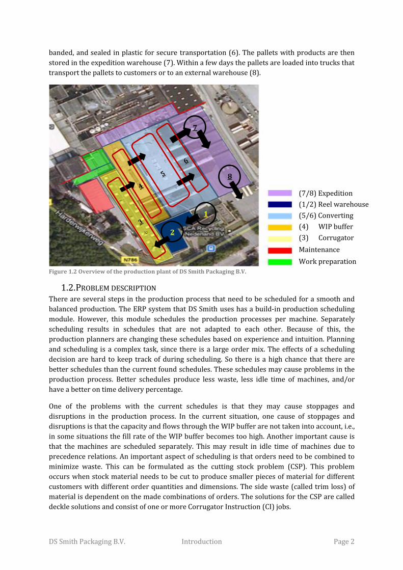
banded, and sealed in plastic for secure transportation (6). The pallets with products are then
stored in the expedition warehouse (7). Within a few days the pallets are loaded into trucks that
transport the pallets to customers or to an external warehouse (8).
Figure 1.2 Overview of the production plant of DS Smith Packaging B.V.
1.2. PROBLEM DESCRIPTION There are several steps in the production process that need to be scheduled for a smooth and
balanced production. The ERP system that DS Smith uses has a build-in production scheduling
module. However, this module schedules the production processes per machine. Separately
scheduling results in schedules that are not adapted to each other. Because of this, the
production planners are changing these schedules based on experience and intuition. Planning
and scheduling is a complex task, since there is a large order mix. The effects of a scheduling
decision are hard to keep track of during scheduling. So there is a high chance that there are
better schedules than the current found schedules. These schedules may cause problems in the
production process. Better schedules produce less waste, less idle time of machines, and/or
have a better on time delivery percentage.
One of the problems with the current schedules is that they may cause stoppages and
disruptions in the production process. In the current situation, one cause of stoppages and
disruptions is that the capacity and flows through the WIP buffer are not taken into account, i.e.,
in some situations the fill rate of the WIP buffer becomes too high. Another important cause is
that the machines are scheduled separately. This may result in idle time of machines due to
precedence relations. An important aspect of scheduling is that orders need to be combined to
minimize waste. This can be formulated as the cutting stock problem (CSP). This problem
occurs when stock material needs to be cut to produce smaller pieces of material for different
customers with different order quantities and dimensions. The side waste (called trim loss) of
material is dependent on the made combinations of orders. The solutions for the CSP are called
deckle solutions and consist of one or more Corrugator Instruction (CI) jobs.
1
7
89
2
(7/8) Expedition
(1/2) Reel warehouse
(5/6) Converting
(4) WIP buffer
(3) Corrugator
Maintenance
Work preparation
DS Smith Packaging B.V. Introduction Page 3
These deckle solutions minimize waste. However, they also cause a decrease in flexibility for
scheduling. The choice for a certain deckle solution has a large impact on the schedules and the
production process. Currently the impact of deckle solutions is not taken into account. We
define the problem that lead to this research in the following way:
“The current approach for production scheduling results in non-optimal schedules that cause
stoppages and disruptions in the production process. This affects the degree in which DS Smith can
meet customer demands and be competitive in the market. ”
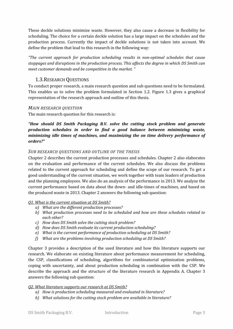
1.3. RESEARCH QUESTIONS To conduct proper research, a main research question and sub questions need to be formulated.
This enables us to solve the problem formulated in Section 1.2. Figure 1.3 gives a graphical
representation of the research approach and outline of this thesis.
MAIN RESEARCH QUESTION The main research question for this research is:
“How should DS Smith Packaging B.V. solve the cutting stock problem and generate
production schedules in order to find a good balance between minimizing waste,
minimizing idle times of machines, and maximizing the on time delivery performance of
orders?”
SUB RESEARCH QUESTIONS AND OUTLINE OF THE THESIS Chapter 2 describes the current production processes and schedules. Chapter 2 also elaborates
on the evaluation and performance of the current schedules. We also discuss the problems
related to the current approach for scheduling and define the scope of our research. To get a
good understanding of the current situation, we work together with team leaders of production
and the planning employees. We also do an analysis of the performance in 2013. We analyze the
current performance based on data about the down- and idle-times of machines, and based on
the produced waste in 2013. Chapter 2 answers the following sub question:
Q1. What is the current situation at DS Smith? a) What are the different production processes? b) What production processes need to be scheduled and how are these schedules related to
each other? c) How does DS Smith solve the cutting stock problem? d) How does DS Smith evaluate its current production scheduling? e) What is the current performance of production scheduling at DS Smith?
f) What are the problems involving production scheduling at DS Smith?
Chapter 3 provides a description of the used literature and how this literature supports our
research. We elaborate on existing literature about performance measurement for scheduling,
the CSP, classifications of scheduling, algorithms for combinatorial optimization problems,
coping with uncertainty, and about production scheduling in combination with the CSP. We
describe the approach and the structure of the literature research in Appendix A. Chapter 3
answers the following sub question:
Q2. What literature supports our research at DS Smith? a) How is production scheduling measured and evaluated in literature?
b) What solutions for the cutting stock problem are available in literature?

DS Smith Packaging B.V. Introduction Page 4
c) What approaches for scheduling are available in literature?
d) How can scheduling and the cutting stock problem be combined?
e) What methods for coping with uncertainty in production scheduling are used in literature?
Chapter 4 formulates the general model and alternative solutions. We use the gathered
information of the literature research for the development of alternatives. Chapter 4 answers
the following sub question:
Q3. What are alternatives for the cutting stock problem and production scheduling at DS Smith?
Chapter 5 provides an evaluation of the alternatives and makes a choice for the best alternative
for DS Smith. Chapter 5 answers the following sub question:
Q4. What is the best alternative for the cutting stock and scheduling problem at DS Smith?
Chapter 6 gives some implementation issues of the proposed alternative. This chapter also
elaborates on parts of the proposed alternative that can be implemented. We also formulate an
evaluation framework for production scheduling. Chapter 6 answers the following the sub
question:
Q5. What are the implementation issues of the proposed alternative?
Finally, Chapter 7 answers the main research question and gives final conclusions and
recommendations.
Figure 1.3 Research approach
Research objectiveResearch methodChapter
Con
clus
ions
Prob
lem
ana
lysi
sSo
lutio
n D
esig
n
Chapter 1 Interviews Problem definition
Chapter 3 Literature study
Q2a Performance
measurement
Q2b Cutting stock problem
Q2c Production scheduling
Q2d Combinations CSP and
production scheduling
Chapter 2Interviews & data
analysis
Q1a-c Current situation
Q1d-f Current performance
Chapter 4Model
developmentQ3 Generate alternatives
Chapter 5 Data analysisQ4 Evaluation of
alternatives
Chapter 6 Q5 Implementation
Chapter 7Conclusions and
recommendations
Q2e Coping with
uncertainty

DS Smith Packaging B.V. Current situation Page 5
2. CURRENT SITUATION This chapter answers the first research question: “What is the current situation at DS Smith?” In
Section 2.1 we describe the general process from order acceptance until shipment of orders to
customers. Section 2.2 describes the corrugator machine and Section 2.3 describes the WIP
buffer (called the Pentek). Section 2.4 describes the converting and expedition department.
Section 2.5 describes the planning department with its scheduling processes and their approach
in solving the CSP. Section 2.6 provides the current performance of scheduling. In Section 2.7 we
elaborate on the problems regarding scheduling of production processes and we define the
scope of this research. Finally, Section 2.8 provides conclusions.
2.1. THE GENERAL PROCESS AT DS SMITH In this section, we describe the process of a customer placing an order until the shipment of the
order to the customer. For a graphical representation of this process, see Figure 2.1. The first
step in the process is an order request of a customer. The sales department checks the Rough
Cut Capacity Planning (RCCP) whether there is enough capacity in the factory for the period that
the customer requested the order. If there is enough capacity, a delivery date is communicated
with the customer. The sales department accepts and releases the order for production. If there
is not enough capacity, the order should be booked in another time period. However, most of
the time the sales employees discuss with the planning employees to look for any opportunity to
produce the order in the requested time period. The sales department also determines the
initial machines on which the orders are produced.
Figure 2.1 Graphical representation of the general process
The planning department can start scheduling when the order is released for production. An
order can be split up in more than one job to minimize waste. We define a job by a task for
production employees to produce a certain amount of an order at a specific time. The planning
employees are responsible for checking the inventory of paper reels (big rolls of paper),
ordering paper reels, making deckle solutions, scheduling CI jobs, and scheduling converting
jobs. In Section 2.5 we elaborate on the tasks of the planning employees.
The first production step is processing jobs on the corrugator machine (see Figure 2.2). Briefly
described, this machine makes corrugated board sheets. Material input for this machine are

DS Smith Packaging B.V. Current situation Page 6
paper reels. Some preparation is needed before the jobs can be processed. One of the
preparation tasks is making sure that the right paper reels are in place. Section 2.2 elaborates
on the production process of the corrugator machine.
Figure 2.2 The corrugator machine
Stacks of corrugated board come out the corrugator machine and are transported with
conveyors and an Automated Guided Vehicle (AGV) to the Pentek (the WIP buffer). The Pentek
itself also consists of conveyors. Section 2.3 describes the Pentek in detail.
The converting step depends on the route of an order; see Figure 2.3 for the different routes.
Corrugated board needs to be produced for every order. The corrugator machine is the first
processing machine in every route. Palletizing is the last step for every route. We divide the
converting machines in two groups. The die cutter machines (Dutch: stans machine) are the first
group and the Flexo Folder Gluers (FFGs) are the second group. The FFGs have a small die
cutting capability and their main function is to fold and glue boxes. The die cutter machines
have a high capability for die cutting and no capability to fold and glue. For boxes that require a
high die cutting capability and need to be glued, the route is according to option A. There are
also boxes that do not need to be glued, but require die cutting. These orders are only processed
on a die cutter (option B). Boxes that only require a small die cutting capability and need to be
glued are processed directly on a FFG machine (option C). A small amount of the orders consist
of “sheet” work. This means that a customer only ordered corrugated board sheets. These
orders only require a corrugator step and a palletizing step (option D).
Figure 2.3 The different product routes

DS Smith Packaging B.V. Current situation Page 7
The products are stacked on each other at both the die cutters and the FFGs. These stacks are
transported via conveyors to the palletizing system that is part of the expedition department. If
an order requires a second converting step (option A), the pallets are transported back to the
Pentek at the moment that this job is scheduled. Otherwise the pallets are placed in the
expedition warehouse. The pallets are then loaded into trucks and within a few days they are
shipped to the customer or to the external warehouse.
2.2. CORRUGATOR MACHINE The corrugator machine makes sheets of corrugated board. Corrugated board consists of
different layers of paper. DS Smith is capable of producing single wall and double wall
corrugated board. Single wall corrugated board consists of three layers of paper: a bottom layer,
a flute layer, and a top layer (see Figure 2.4). Double wall corrugated board has two flute layers
(see Figure 2.5).
For each flute different kinds of corrugating rolls are needed. The corrugating rolls make the
shape of the flute (see Figure 2.6). The first part of the machine makes corrugated board. The
machine is capable of making eight different kinds of corrugated board. Four single wall with a
B-, C-, E-, or R-flute and four double wall with flute combinations B-E, E-B, B-C, or E-E. Moreover,
there are also quality differences because of different kinds of paper. The quality of the
corrugated board is called the board grade.
The next part of the machine makes the creases and cuts the corrugated board in width and
length. Up to seven sheets can be cut next to each other. Two jobs can be produced next to each
other that are of the same board grade. This is an important feature of the machine that enables
minimizing waste of corrugated board. See Figure 2.7 for a simplified representation of the
different stages of the corrugator machine.
Figure 2.7 Stages of the corrugating process (Rodriguez & Vecchietti, 2013). In this example of a CI job where two sheets of order i1 and two sheets of order i2 are produced next to each other.
Figure 2.4 Single wall corrugated board
Figure 2.5 Double wall corrugated board
Figure 2.6 Corrugating rolls
Order i1
Order i2

DS Smith Packaging B.V. Current situation Page 8
The possibility to combine orders makes scheduling more complex. Making the combinations of
orders for the corrugator machine is called making a deckle solution. In Section 2.4 we explain
how these deckle solutions are made and evaluated. The corrugator machine automatically
stacks the corrugated board sheets and finally these stacks are transported to the Pentek
(Figure 2.8).
ISSUES There are several issues regarding the corrugator machine.
Waste: The planning department makes schedules that ensure producing minimal
waste. This can result in a deckle solution and corrugator schedule that has a lot of
changeovers and require more time for production.
Down/Idle time: Changeovers result in set-up time in the case of a corrugator roll
change. Also just before and after the change, the speed of the machine is less. Effective
production time and speed is lost when doing changeovers. Moreover, it is easier to
maintain the right quality when producing large runs of the same quality. The
corrugator machine is the bottleneck machine. So down/idle time of this machine
results in a reduction of throughput of the whole factory.
Workload: Having a lot of changeovers result in a higher workload for the lift truck
driver, who needs to get the reels out of the reel warehouse for every changeover. Left
over reels must be transported back to the reel warehouse.
Figure 2.8 Transporting stacks to the Pentek Figure 2.9 Conveyors of the Pentek
2.3. THE PENTEK (WIP BUFFER) The WIP buffer, from now on called the Pentek, has an important role in the production process.
After the production at the corrugator machine, the stacks of corrugated board sheets are
transported to the Pentek with an AGV (AGV1). The Pentek is used as a buffer to enable a
smooth production process, but is also used as drying area. Some board grades require a certain
drying time before it can be processed on a converting machine. The stacks are transported
with a second AGV (AGV2) to the converting machines. The Pentek consists of 31 automated
conveyors each with a length of 16.5 meter (see Figure 2.9). When the utility of the Pentek is
higher than 75% the corrugator machine is shut down. High utilization of the Pentek results in
disruptions and stoppages in the whole production process.
Figure 2.10 gives an overview of how the Pentek is connected with the machines. The large blue
block on the left is the corrugator machine. There are four output conveyors next to the
corrugator machine. All the yellow/orange blocks are automated conveyors, the two AGVs can
only travel vertically between the arrows, and the green blocks are the converting machines.

DS Smith Packaging B.V. Current situation Page 9
AGV1 picks up stacks from the output conveyors of the corrugator machine and places the
stacks on one of the conveyors of the Pentek. AGV2 picks up the stacks from the conveyors and
transports them to the input conveyors of the converting machines. The sequence in which the
stacks are placed on the conveyors are of great importance. Once a stack is placed on a
conveyor, the stacks are handled according to the FIFO rule. There is a possibility to shuffle the
stacks. However, this costs capacity of AGV2 that transports the stacks to the machines. So
shuffling of stacks can result in congestion in the Pentek due to unavailability of AGV2. Another
drawback of shuffling is that the Pentek can become a “big mess”. There is a chance that stacks
of the same order are placed all over the Pentek. This can result in further shuffling of stacks in
the Pentek.
Figure 2.10 Overview of the Pentek
ALLOCATION OF THE STACKS TO A CONVEYOR For monitoring and controlling the AGVs and the Pentek itself, the company uses a separate IT
system. Once the stacks of corrugated board sheets are leaving the corrugator machine, the
stacks enter the Pentek system and are linked to a Production Order number (PO number). Via
this PO number the stacks are linked to a machine on which they need to be processed.
On entrance, the stacks are allocated to a certain conveyor number. This is done based on the
width of the stacks, because the conveyors have different widths. Also the system tries to place
stacks of the same order on the same conveyor.
TRANSPORTING STACKS FROM THE CONVEYOR TO THE MACHINES AGV2 is controlled based on the fill rates of the conveyors that are placed in front of the
machines. On each conveyor there are sensors that measure the fill rate. AGV2 first picks up
stacks for machines that have the lowest fill rate. When a conveyor is full, the AGV cannot
transport stacks to that conveyor. If there are no possibilities for the AGV to transport any
stacks from the Pentek to the machines, it looks for shuffling tasks. This can be done by using a
DS Smith Packaging B.V. Current situation Page 10
retrieving conveyor. One conveyor in the Pentek is used for retrieving. This conveyor transports
the stacks back into the direction of the corrugator machine. These stacks are then picked up
with AGV1. This AGV brings the stacks to another conveyor.
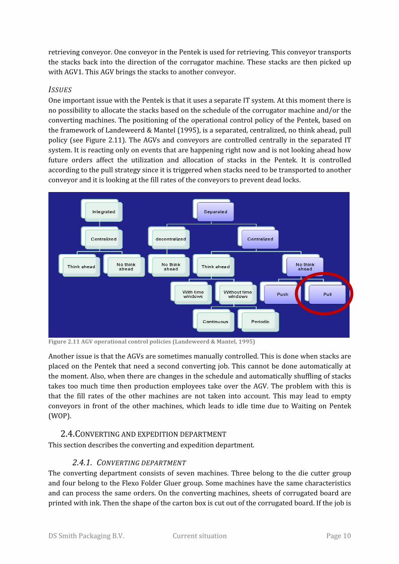
ISSUES One important issue with the Pentek is that it uses a separate IT system. At this moment there is
no possibility to allocate the stacks based on the schedule of the corrugator machine and/or the
converting machines. The positioning of the operational control policy of the Pentek, based on
the framework of Landeweerd & Mantel (1995), is a separated, centralized, no think ahead, pull
policy (see Figure 2.11). The AGVs and conveyors are controlled centrally in the separated IT
system. It is reacting only on events that are happening right now and is not looking ahead how
future orders affect the utilization and allocation of stacks in the Pentek. It is controlled
according to the pull strategy since it is triggered when stacks need to be transported to another
conveyor and it is looking at the fill rates of the conveyors to prevent dead locks.
Figure 2.11 AGV operational control policies (Landeweerd & Mantel, 1995)
Another issue is that the AGVs are sometimes manually controlled. This is done when stacks are
placed on the Pentek that need a second converting job. This cannot be done automatically at
the moment. Also, when there are changes in the schedule and automatically shuffling of stacks
takes too much time then production employees take over the AGV. The problem with this is
that the fill rates of the other machines are not taken into account. This may lead to empty
conveyors in front of the other machines, which leads to idle time due to Waiting on Pentek
(WOP).
2.4. CONVERTING AND EXPEDITION DEPARTMENT This section describes the converting and expedition department.
2.4.1. CONVERTING DEPARTMENT The converting department consists of seven machines. Three belong to the die cutter group
and four belong to the Flexo Folder Gluer group. Some machines have the same characteristics
and can process the same orders. On the converting machines, sheets of corrugated board are
printed with ink. Then the shape of the carton box is cut out of the corrugated board. If the job is

DS Smith Packaging B.V. Current situation Page 11
processed on one of the FFGs, then the boxes are
also folded and glued. At the end of each
machine the carton boxes are stacked on each
other. The stacks are transported to a palletizing
area via automated conveyors (see Figure 2.12).
The characteristics of the machines are
summarized in Table 2.1. We do not give a
detailed description of the different types of
machines. This is not relevant for our research
and understanding of the process.
Machine number Supplier Number of colors Type
728
confidential
729 735 419 425 426 436 Table 2.1 Converting machines
The number of colors that a job requires determines to what degree the machines are
interchangeable. If an order needs a converting step on a FFG and has three colors it can be
produced on three machines (425, 426, and 436). If it has four colors it can only be produced by
the 425. The dimensions of the corrugated board also determine what machine can be used. The
machines have different production speeds. The speed of a machine depends on several aspects:
sheet dimensions, number of colors, and cardboard quality. The ERP-system keeps track of the
historical production speeds per order. The average of these speeds is used to determine the
production time of an order.
ISSUES One issue related to scheduling is that the production department has different objectives than
the planning employees. The production employees want to produce in such way that set-ups
are the easiest. So they want schedules that take into account sheet dimensions, colors, and also
which dies are used. However, the planning employees do not take this into account. Delivery
dates and a smooth and balanced production process are their objectives. In some situations
this results in changes of the converting schedule, e.g., a certain change in schedule results in
less or easier set-up for production and cause no problems in the process. However, not all
effects of scheduling changes are known and visible.
2.4.2. EXPEDITION DEPARTMENT The expedition department is responsible for palletizing the finished and semi-finished
products. This is done automatically with machines that press the products on pallets, banding
the pallets, and if necessary sealing the pallets in plastic. If a second converting job is needed,
the pallets are transported back to the Pentek or stored for a short time in the warehouse.
Transporting pallets back into the Pentek is done by pushing the semi-finished products from
the pallets on a conveyor. The conveyor used for this is not an automated conveyor. Therefore,
Figure 2.12 Stacks of finished products

DS Smith Packaging B.V. Current situation Page 12
AGV2 needs to be controlled manually to place the semi-finished products on another conveyor
of the Pentek or in front of the right machine.
ISSUES The expedition department is not taken into account with scheduling. However, the expedition
department may become a bottleneck when all the seven converting machine are producing on
full speed. When one of the machines of the expedition department is down, the whole
expedition department is down since the machines are serially positioned. This does not happen
frequently, so this is not an issue that we need to take into account.
2.5. PLANNING DEPARTMENT In this section we describe the tasks of the planning employees. The tasks are split up in making
deckle solutions, CI job scheduling, converting scheduling, expedition scheduling, and
monitoring and controlling the schedules and Pentek. The schedules are made for 20-30 hours
in advance.
2.5.1. MAKING DECKLE SOLUTIONS / CSP Making a deckle solution is the process of combining corrugator jobs in order to minimize
waste. As mentioned earlier, this can be formulated as the CSP. The CSP is applicable in many
industries. Also the literature about the CSP is extensive; Sweeney and Paternoster (1991) have
identified more than 500 papers about the CSP.
Figure 2.13 Example of a deckle solution that consist of three CI jobs (c1, c2, and c3), uses two paper widths
(w1 and w2), and produces sheets for three orders (A, B, and C). The red and green shaded areas are trim loss.
See Figure 2.13 for an example of a deckle solution. This deckle solution consists of three CI jobs
(in literature called cutting patterns or patterns). The first CI job (c1) produces three sheets next
to each other of the same order (C-C-C) with a paper reel of width w1, the second (A-C-C) and
third (A-A-B) CI job (c2 and c3) produce sheets of two different orders with a paper reel of width
w2. The red and green shaded areas are the trim loss waste of corrugated board of the Deckle
solution. These deckle solutions are generated via a built-in Integer Linear Program (ILP).
Before running the ILP, parameters and constraints need to be filled in about paper dimensions,
minimum trim los, maximum trim loss, minimum CI job run length, minimum run length per
paper width, and the minimum and maximum order quantity that may be delivered to the
customer. The program shows several feasible solutions. The planning employee chooses a
solution that fits best the preferences of the production employees and that also has a low trim
loss.
Paper reel of
width w2
Paper reel
of width w1
CI job c2 CI job c1 CI job c3
DS Smith Packaging B.V. Current situation Page 13
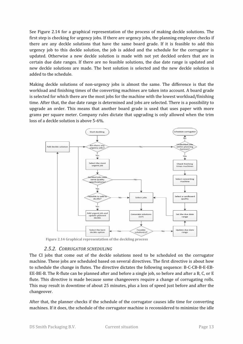
See Figure 2.14 for a graphical representation of the process of making deckle solutions. The
first step is checking for urgency jobs. If there are urgency jobs, the planning employee checks if
there are any deckle solutions that have the same board grade. If it is feasible to add this
urgency job to this deckle solution, the job is added and the schedule for the corrugator is
updated. Otherwise a new deckle solution is made with not yet deckled orders that are in
certain due date ranges. If there are no feasible solutions, the due date range is updated and
new deckle solutions are made. The best solution is selected and the new deckle solution is
added to the schedule.
Making deckle solutions of non-urgency jobs is almost the same. The difference is that the
workload and finishing times of the converting machines are taken into account. A board grade
is selected for which there are the most jobs for the machine with the lowest workload/finishing
time. After that, the due date range is determined and jobs are selected. There is a possibility to
upgrade an order. This means that another board grade is used that uses paper with more
grams per square meter. Company rules dictate that upgrading is only allowed when the trim
loss of a deckle solution is above 5-6%.
Figure 2.14 Graphical representation of the deckling process
2.5.2. CORRUGATOR SCHEDULING The CI jobs that come out of the deckle solutions need to be scheduled on the corrugator
machine. These jobs are scheduled based on several directives. The first directive is about how
to schedule the change in flutes. The directive dictates the following sequence: B-C-CB-B-E-EB-
EE-BE-B. The R-flute can be planned after and before a single job, so before and after a B, C, or E
flute. This directive is made because some changeovers require a change of corrugating rolls.
This may result in downtime of about 25 minutes, plus a loss of speed just before and after the
changeover.
After that, the planner checks if the schedule of the corrugator causes idle time for converting
machines. If it does, the schedule of the corrugator machine is reconsidered to minimize the idle

DS Smith Packaging B.V. Current situation Page 14
time. When it is not possible to prevent idle time, the machines that have large idle times are
taken out of the schedule for production.
The second directive dictates that jobs with the same flute and board grade are scheduled in
descending order based on trim loss. This is done because jobs with small trim loss require a
higher accuracy. Scheduling them in the beginning can cause problems since the first job of a
certain quality requires some fine tuning. The third directive dictates that large jobs are planned
first and the fourth directive is about the paper width. The corrugator jobs with the largest
paper width should be produced first within a deckle solution.
2.5.3. CONVERTING SCHEDULING After the CI jobs are scheduled, the estimated arrival times at the Pentek are known and the
converting jobs are scheduled. The jobs are first planned based on the FIFO rule. After that, the
workloads and finishing times of converting machines are checked. If the workload of a machine
is too high, jobs of that machine are scheduled on an interchangeable machine. The initial
machine is determined by the sales department as mentioned in Section 2.1. If the workload is
too low, this machine probably becomes idle. Jobs on interchangeable machines are then
scheduled on this idle machine. If this is not possible or insufficient, the schedule of the
corrugator machine can be changed to balance the workload. This can be done by changing the
sequence of the deckle solutions.
The directives for converting scheduling are different from the directives of corrugating
scheduling. The most important directive is that due dates are met (Directive 1). So if the FIFO
rule results in jobs that are not finished before the due date, the schedule needs to be changed.
The second directive is about job characteristics. If there are jobs with the same characteristics,
then these jobs are scheduled after each other to minimize set up times. The third directive
dictates that jobs of the same board grade should be scheduled after each other.
Scheduling of converting jobs is done after making deckle solutions and scheduling of the CI
jobs. However, the workload of converting machines is already taken into account when making
deckle solutions and scheduling the CI jobs to prevent many changes afterwards.
2.5.4. EXPEDITION SCHEDULING The expedition schedule is made one day ahead. Orders are combined to optimize truck
utilization and transportation costs. The expedition department benefits from reliable
production schedules. If there are changes in production schedules, then there is a possibility
that the schedule of expedition also changes. If this is not communicated or is done at the last
moment, trucks need to wait or are not full. This results in higher costs of transportation and
the on time delivery decreases.
2.5.5. MONITORING AND CONTROLLING THE CURRENT SCHEDULES AND PENTEK Since there is uncertainty, it is necessary to monitor and control the schedules. A small change
in one schedule may cause other schedules to change as well. These changes may be a cause of
downtime, idle time, maintenance, unavailability of workforce, unavailability of dies, etcetera. In
order to keep a balanced and smooth production, these changes need to be evaluated and
rescheduling may be needed. Utilization of the Pentek also needs to be monitored since this can
cause both the corrugator and converting machines to become idle. Another reason for

DS Smith Packaging B.V. Current situation Page 15
monitoring and controlling the Pentek is that it gives a good picture of the workload for the
converting machines for the coming hours.
2.6. CURRENT EVALUATION AND PERFORMANCE OF SCHEDULING The performance of production is currently evaluated based on several performance indicators.
Some of these indicators can also be used for the evaluation of the performance of scheduling
since they are directly a result of the schedules.
TRIM LOSS This is the performance indicator that measures the quality of the deckle solutions. Trim loss is
waste of corrugated board at the corrugator machine at both sides of the paper, measured in
percentage of the total width of the paper. The total trim loss was in 2013 (the target confidential
trim loss is 3.6%). We conclude that the performance of the deckle solutions is on target.
However, when we take into account the waste of a side job, the total waste was in confidential
2013. A side job is trim loss that cannot be drained by the corrugator machine. A new
corrugator job is created to transport the waste (the side job) to the Pentek.
IN FULL (IF) Each order has minimum and maximum quantities. The standard tolerances in the packaging
industry are -10% and +10% of the ordered quantity. The In Full indicator measures how many
orders are delivered within these minimum and maximum order quantities. In 2013 the In Full
percentage was while the target was 90%. It is hard to predict the amount of waste confidential
produced for a specific order. Also there are company directives that dictate that the planned
quantity must be between 104% and 106% of the ordered quantity.
ON TIME DELIVERY (OT) This indicator measures how many orders are delivered on time. Orders that are not delivered
In Full but are on time are also counted as delivered on time. In 2013 the On Time Delivery
percentage was where the target was 96%. confidential
ON TIME IN FULL DELIVERY (OTIF) This indicator measures how many orders are both In Full and On Time delivered. The target for
this indicator is 85% while in 2013 only is reached. This indicator is not an indicator confidential
that stands for itself. It is a combination of the On Time Delivery and the In Full delivery.
WAITING ON PENTEK (WOP) This is the performance indicator that measures how much time a converting machine was idle
because it needed to wait on sheets. This is a result of the Pentek that could not deliver sheets in
time. In 2013, the converting machines needed to wait in total days on the Pentek. confidential
WAITING ON CORRUGATOR (WOC) Waiting on corrugator is the indicator of idle time of the converting machines, because the
corrugator machine could not make sheets in time for the converting machines. The total idle
time of the converting machines because of waiting on corrugator was days in 2013. confidential
IDLE TIME OF CORRUGATOR CAUSED BY A FULL PENTEK This indicator is based on the total registered idle time caused by a full Pentek for the
corrugator machine as percentage of the total available time of the machine. The total idle time

DS Smith Packaging B.V. Current situation Page 16
at the corrugator machine caused by a full Pentek in 2013 was days. Per idle time confidential
occasion, the average idle time was around two hours. The available production time in 2013
was days. So the corrugator machine was of the time idle due to a full Pentek. confidential confidential
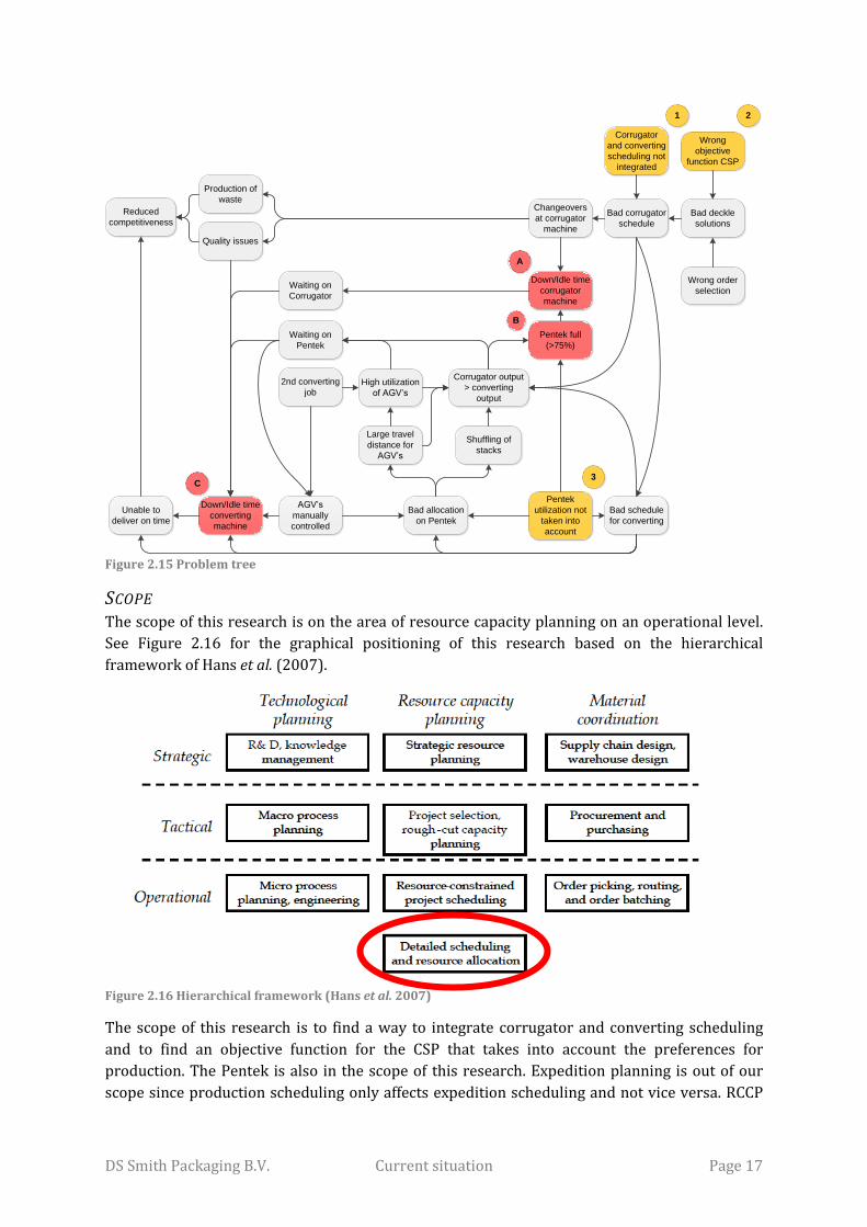
2.7. PROBLEM IDENTIFICATION In this section we identify the problems that are related to scheduling. There are three main
problems that have the highest impact on the production process. These are idle/down times of
the corrugator machine and converting machines and the high utilization of the Pentek. The
problems are shown in a problem tree (see Figure 2.15).
A: DOWN/IDLE TIME OF THE CORRUGATOR MACHINE Down or idle time of the corrugator machine can be caused by different situations. However,
only two of the causes are related to scheduling. The first one is that there is a schedule that
needs changeovers that are not according to the directives of corrugator scheduling. These
changeovers cause the corrugator machine to have downtime. Another cause of idle/down time
is that the utilization of the Pentek is above 75%. If the Pentek is utilized above 75% it is not
working properly and the corrugator machine is shut down. Since the corrugator machine is the
bottleneck of the company, downtime or idle time results in an overall lower throughput.
B: HIGH UTILIZATION OF THE PENTEK (>75%) A high utilization of the Pentek has several causes. The first cause is that the corrugator machine
is producing more than the converting machines. A bad allocation of the stacks in the Pentek
may be a cause for the low output of the converting machines. This causes the AGVs to travel
long distances and also results in shuffling of stacks.
With the current way of scheduling the limitations of the Pentek are not taken into account. This
causes a high variability in utilization level of the Pentek. If the Pentek has a low utilization,
converting machines may become idle due to waiting on corrugator. A high utilization of the
Pentek may result in downtime of the corrugator machine. Other reasons are changes in the
converting schedules and manually controlling the AGVs.
C: DOWN/ IDLE TIME OF THE CONVERTING MACHINE The reduced throughput of the Pentek may result in idle/down time of the converting machines.
Low throughput causes machines to wait on sheets, i.e., the AGVs cannot supply the machines in
time. Another possible cause for idle time is that there are no sheets in the Pentek. This may be
a result of downtime at the corrugator machine or a “bad” schedule.
Another cause of the downtime at the converting machine may be that a second processing job
for converting is needed. Time is needed to get the stacks in the Pentek and also the AGVs need
to be controlled manually. People are needed for this and if there are none available the
operators need to do it themselves. This causes the converting machine to become idle.
MAIN CAUSES The main causes of the problems are that corrugator and converting scheduling is not
integrated (1). Next to this, DS Smith is using an objective function for solving the CSP that only
takes into account trim loss(2). The last main cause is that the utilization of the Pentek is not
taken into account (3). This results in schedules that are not robust and not reliable.
DS Smith Packaging B.V. Current situation Page 17
Figure 2.15 Problem tree
SCOPE The scope of this research is on the area of resource capacity planning on an operational level.
See Figure 2.16 for the graphical positioning of this research based on the hierarchical
framework of Hans et al. (2007).
Figure 2.16 Hierarchical framework (Hans et al. 2007)
The scope of this research is to find a way to integrate corrugator and converting scheduling
and to find an objective function for the CSP that takes into account the preferences for
production. The Pentek is also in the scope of this research. Expedition planning is out of our
scope since production scheduling only affects expedition scheduling and not vice versa. RCCP
Pentek full
(>75%)
Waiting on
Pentek
Down/Idle time
converting
machine
AGV’s
manually
controlled
Bad allocation
on Pentek
Large travel
distance for
AGV’s
Corrugator
and converting
scheduling not
integrated
Changeovers
at corrugator
machine
Down/Idle time
corrugator
machine
Quality issues
Production of
waste
Corrugator output
> converting
output
2nd converting
job
Pentek
utilization not
taken into
account
Unable to
deliver on time
Reduced
competitiveness
Bad schedule
for converting
Shuffling of
stacks
High utilization
of AGV’s
Waiting on
Corrugator
C
A
B
1
3
Bad corrugator
schedule
Bad deckle
solutions
Wrong
objective
function CSP
Wrong order
selection
2

DS Smith Packaging B.V. Current situation Page 18
and order acceptance are on a tactical level and not on an operational level. Although both affect
production scheduling, we exclude it from the scope. If we would include it in the scope, the
problem would become more complex. We decided to exclude RCCP and order acceptance to
keep the research manageable. Upgrading of board grades of orders is also excluded from the
scope of this research. Upgrading is a last resort if the trim loss is too large and is not preferred
because the customer ordered a different board grade, i.e., the demands of the customer are not
met if a board grade is upgraded.
DELIVERABLES The deliverable of this research is a solution that supports the tasks of the production planners.
We need to model the process of order selection, solving the CSP, scheduling the corrugator
machine, scheduling the converting machines, and monitoring and controlling the Pentek. The
different tasks are first modelled as separate modules. Alternative solutions are developed
where modules are integrated or closely linked. The aim is not to implement this solution. The
outcomes of this research are used to give new insights in the planning and scheduling
processes at DS Smith. These insights may be used to implement parts of the solution in the
current ERP system of DS Smith to improve planning and scheduling.
2.8. CONCLUSIONS In this chapter we described the current situation at DS Smith. First jobs are processed on the
corrugator machine and then transported to the Pentek. After that, one or two converting jobs
are performed. Finally, the pallets with the finished products are palletized and transported to
customers or to the external warehouse.
Orders need to be combined for the corrugator machine. This is called making deckle solutions
and can be formulated as the cutting stock problem (CSP). The choice for a deckle solution has a
high impact on the schedules of the corrugator machine and the converting machines. Currently,
the preferences of production are only taken into account for a small amount when making and
selecting the deckle solutions. This results in problems in the production process. Another cause
for problems in the production process is that corrugator and convertor scheduling is not
integrated. Finally, the Pentek with its limitations is also not taken into account.
The scope of this research is to find a way to integrate corrugator and convertor scheduling and
to find an objective function for the CSP that takes into account preferences of production. This
research needs to deliver a solution that supports the tasks of the production planners in
different modules. Alternative solutions are developed where these modules are integrated or
closely linked. To model the tasks of the production planners in the best way, we do a literature
review on the CSP, performance measurement, and scheduling techniques in Chapter 3.

DS Smith Packaging B.V. Theoretical framework Page 19
3. THEORETICAL FRAMEWORK In Chapter 2 we elaborated on the current situation at DS Smith and defined the main problems,
the scope, and the deliverables of this research. In this chapter we outline the theoretical
framework for this research by answering the second research question: “What literature
supports our research at DS Smith?”
First we describe literature about performance measurement for production scheduling in
Section 3.1. Second, Section 3.2 describes the CSP and the solutions for it in the corrugated
board industry. In Section 3.3 we elaborate on different classifications for production
scheduling and what classification is applicable for DS Smith. Section 3.4 provides algorithms
that are capable of solving hard combinatorial optimization problems. Section 3.5 describes
combinations of the CSP with production scheduling. Section 3.6 describes approaches for
coping with uncertainty. Finally, Section 3.7 provides conclusions.
3.1. PERFORMANCE MEASUREMENT We need to know how we can evaluate and measure the performance of a schedule in order to
determine which scheduling approach or algorithm is the best for DS Smith. A performance
measure can be defined as “a metric used to quantify the efficiency and/or effectiveness of an
action” (Neely et al., 2005). In our case we want to quantify the effectiveness of a production
schedule. Kempf et al. (2000) mention the importance of quality measurement of a schedule.
They state that a clear understanding of the quality of a schedule is essential for a successful
implementation of a scheduling system.
3.1.1. PERFORMANCE INDICATORS We need to define performance indicators of a production schedule in order to assess the
quality of a certain schedule. Hoogeveen (2005) state that if only one indicator is used, the
schedule is likely to be unbalanced, no matter what indicator is considered. The following
performance indicators are widely used in literature (Hsu, 2006; Hoogeveen, 2005; De Snoo et
al., 2011; Bandinelli et al., 2005):
- Maximum completion time - Maximum tardiness - Maximum earliness - Total completion time - Average tardiness - Total earliness - Maximum lateness - Total tardiness - Total number of tardy jobs - Average lateness - Maximum cost - Total waiting time - Total flow time/cycle time Indicators that can directly be calculated from scheduling objects (set of jobs, time assignments
and machines) are called atomic metrics (Kempf et al., 2000). These atomic metrics quantify
how much time each scheduling object is in each possible state. Examples of states of a machine
are: busy, setup, maintenance, idle, and down. Examples of states of a job are: in process, in
transport, on hold or idle. These atomic metrics can also be used as performance indicators. For
example, the percentage of time a machine is idle and/or down.
3.1.2. MULTI-CRITERIA SCHEDULING Only using one of the many performance indicators is not sufficient for evaluating a schedule. So
we need a way to evaluate a schedule based on multiple criteria. Hoogeveen (2005) mentions
two approaches to deal with multiple criteria. The first one is the hierarchical or lexicographical
optimization approach. This approach selects one performance criteria, say f, which is the most

DS Smith Packaging B.V. Theoretical framework Page 20
important. A set of optimal schedules based on f is generated. From this set of optimum
schedules, the schedule is selected that has the best performance on the other criteria.
The second approach is simultaneous optimization, where the performance criteria are
evaluated simultaneously. Simultaneous optimization is divided in three different approaches: a
priori optimization, interactive optimization, and a posteriori optimization (Fry et al., 1989;
Evans, 1984).
A priori optimization: With this approach all the criteria are taken together in one
objective function. This function can be linear, but also quadratic, or any other form. A
drawback of this approach is that it is hard to define the parameters of the objective
function. Another drawback is that minimizing the objective function is most of the time
NP-hard for scheduling problems.
Interactive optimization: This approach uses the expertise of the decision maker. One or
more schedules are already generated and the decision maker must select the one that is
preferable and in which direction the search should continue.
A posteriori optimization: This last approach is used when the objective function is not
known. A set of feasible solutions is presented to the decision maker and he/she must
choose the one that is the best according to him/her.
A problem with using multiple criteria is that they can be related to each other (Kempf et al.,
2000). For example: Maximizing machine utilization may result in an increase in WIP, while
minimizing WIP is another objective. Another problem with using multiple criteria is that it
results in an increase in complexity of the scheduling problem.
3.1.3. EVALUATION FRAMEWORK Bandinelli et al. (2005) propose a framework for the evaluation and comparison of production
schedules. The framework is based on three layers: The effectiveness domain, the robustness
domain, and the flexibility domain.
Effectiveness domain: This domain evaluates the effectiveness of the company according
to the control of a scheduling solution. It describes how the whole manufacturing system
works and not just the efficiency of machines and workforce.
Robustness domain: This domain consists of indicators that measure the robustness
level of scheduling solutions. Robustness is defined as the ability of a scheduling system
to perform with graceful degradation of the performance in the face of external or
internal disruptions.
Flexibility domain: This domain measures how easy a scheduling system can be
implemented in a different production environment or when the environment changes.
De Snoo et al. (2011) distinct between product and process related performance. Product
performance is about how well internal and external constraints are fulfilled and process
performance is about the reliability, flexibility, response speed, and communication and
harmonization capabilities of the schedulers. De Snoo et al. (2011) propose a new scheduling
performance measurement framework that consists of four parts, see Figure 3.1. The first part
consists of criteria focused on the scheduling product. The second part consists of criteria
focused on the scheduling process. The third part consists of indirect scheduling performance
criteria and the last part consists of influencing factors.

DS Smith Packaging B.V. Theoretical framework Page 21
The framework of Bandinelli et al. (2005) made a clear distinction between different domains of
scheduling. Besides measuring the performance of a schedule they also evaluate how the
schedule or scheduling method performs when disruptions occur and if it could be implemented
in another environment. De Snoo et al. (2011) are more focused on scheduling performance in a
certain company/organization. They do not measure how flexible the scheduling is and the
robustness is only incorporated in one performance indicator (6).
Criteria focussed on the scheduling product Criteria focussed on the scheduling problems Indirect scheduling performance criteria Influencing factors
Scheduling performance criteria
1. Scheduling errors
2. Costs of execution of the schedule
3. Fulfilment of constraints and
commitments made to external partners
4. Fulfilment of resource utilization
constraints
5. Fulfilment of preferences and wishes of
employees using the schedules
6. Schedule robustness/ information
completeness
7. Information presentation and clarity
8. Timeliness of initial release
9. Reliability of initial release
10. Flexibility of schedule adaption
11. Accessibility of schedulers
12. Communication quality
13. Harmonization quality
14. Cost and efficiency of the scheduling
process
15. Realized performance of the scheduled
process
16. Complaints and feedback from
schedule users
17. Organizational planning structure
18. Scheduler knowledge
19. Information technology
20. Information quality
21. Complexity and uncertainty
Figure 3.1 Scheduling performance measurement framework (De Snoo et al., 2011)
3.1.4. DIFFICULTIES WITH PERFORMANCE MEASUREMENT OF SCHEDULING Measuring the performance of a schedule is not easy. One difficulty with scheduling is how to
cope with uncertainty. Aytug et al. (2005) address that it is unlikely, in any environment other
than a tightly integrated automated situation, that a predictive schedule is executed exactly as
planned. A schedule developed under certain assumptions (such as no disruptions will occur) is
called a predictive schedule. The schedule may be changed when disruptions occur. This is
referred to as reactive scheduling or rescheduling.
Aytug et al. (2005) identify three dimensions of uncertainty: cause, context, and impact. Cause
can be seen as an object, for example: material, process, resource, tooling or personnel. An
object is in a certain state, for example: ready, not ready, high quality, low quality, damaged,
healthy, etcetera. The context is about how the environmental situation is at the time of the
scheduled event. A situation can be either context-free or context-sensitive. A context-free
situation does not need any additional information on the situation (the situation is always the
same) and a context-sensitive situation does need additional information for decision making
(the situation changes). The result of uncertainty, for example disruptions in the production
process, is referred to as the impact of uncertainty. Impact can be categorized as time, material,
quality, independent or dependent, and context-free or context-sensitive. The impact of
uncertainty on other jobs and activities is referred to as dependent or independent. So if
uncertainty of one job has an impact on other jobs it is dependent. Inclusion is an additional
dimension of uncertainty and it is about how to cope with uncertainty, in a predictive or in a
reactive way.
Another difficulty is that most performance measures only consider all the jobs at once. They do
not consider the individual needs of a specific job, while customers may have different
requirements for their orders (Hsu, 2006) .

DS Smith Packaging B.V. Theoretical framework Page 22
3.2. CUTTING STOCK PROBLEM The CSP is a widely researched problem, with many applications. In this section we give
solutions that are available in the literature for the corrugated board industry.
3.2.1. TYPOLOGY OF THE CUTTING STOCK PROBLEM Dyckhoff (1990) proposes a typology for cutting and packing problems. Dyckhoff (1990)
distinguishes between the dimensionality, kind of assignment, assortment of large objects, and
assortment of small items. We underline the typology that is applicable for the situation at DS
Smith.
DIMENSIONALITY Dimensionality is the most important characteristic of the typology. It refers to the number of
dimensions necessary to describe the geometry of the patterns. The elementary types are:
(1) One-dimensional: only the width of patterns is considered.
(2) Two-dimensional: both the width and length in patterns are considered.
(3) Three-dimensional: the width, length, and height of patterns are considered
(applicable for packing problems).
(N) Multi-dimensional: this is a three dimensional problem with time as fourth
dimension.
This research only consists of one-dimensional problems, since trim loss minimization only
takes into account the width of cutting patterns.
KIND OF ASSIGNMENT For the classification it is important to know what kind of assignment is needed. Two possible
kinds of assignments are possible. The first assignment is a selection of items (orders) that need
to be assigned to all the available large objects (paper reels). This is the case when there are
limited raw materials and jobs need to be selected for production. The second assigns all items
to a selection of large objects. In the situation of DS Smith there are sufficient raw materials and
the raw materials to use need to be selected. So, the second kind of assignment is applicable for
the trim loss optimization at DS Smith.
(B) All objects and a selection of items
(V) A selection of objects and all items
ASSORTMENT OF LARGE OBJECTS The assortment of large objects means in our case the assortment of the paper reels. Three
types of assortments are distinguished: one object, identical figure, and different figures. With
one object is meant that the small items (orders) need to be cut out of one large object (paper
reel). With identical figure is meant that the small items need to be cut out of multiple large
objects and these objects are identical. In the case of DS Smith we deal with different figures, i.e.,
the orders need to be cut out of multiple paper reels that are of different paper qualities and
different widths.
(O) One object
(I) Identical figure
(D) Different figure

DS Smith Packaging B.V. Theoretical framework Page 23
ASSORTMENT OF SMALL ITEMS The assortment of small items (orders) is the output of the process. So the pieces that come out
of the large input objects that need to be cut. Four types of assortments are possible for the
small items:
(F) Few items
(M) Many items of different figures
(R) Many items of relatively few different figures (non-congruent)
(C) Congruent figures
With this research we cope with many orders and the figures are always rectangles but not
congruent in most cases. So we deal with many items of relatively few different figures. With
congruent figures is meant that the figures all have corresponding sides and angles. We
conclude that our CSP can be formulated as a 1/V/D/R CSP.
3.2.2. SOLUTION APPROACHES FOR THE CUTTING STOCK PROBLEM The work of Gilmore & Gomory (1961; 1963) was the first significant work on the area of
solving the one-dimensional CSP. They solved the CSP by solving a knapsack problem to
determine the next pattern to enter the Linear Program (LP) basis. In this way not all possible
patterns need to be considered. However, in most practical situations we need an Integer Linear
Program (ILP) instead of an LP. The number of products cut out must be an integer number or
we need auxiliary integer/binary variables when including constraints. Haessler and Sweeney
(1991) formulated the following ILP model for a one-dimensional CSP (1/V/I/R). With this
model, rli is the lower bound of the order requirement and rui is the upper bound of the order
requirement. UW is the width of a paper reel. ai,j is the number of sheets to be cut next to each
other of width wi from cutting pattern j. Xj is the total run length of cutting pattern j. The
objective function is to minimize the total trim loss.
z: *j j
j
Min t X
Subject to:
, * ii i j j
j
rl a X
, * ii i j j
j
ru a X
, * ji j i
i
a w uw
, * jj i j i
i
t uw a w
0 and integerjX
This formulation only takes into account the trim loss. However, in most situations other factors
need to be considered as well. Moreover, this formulation only takes into account one paper
width, while in many situations multiple paper widths are available. To be applicable for our
research we must formulate the ILP model for a 1/V/D/R model instead of the 1/V/I/R model
proposed by Haessler and Sweeney (1991).
Indices: i = order number j = pattern number Parameters: ai,j = # sheets of order i in pattern j rli = minimum order quantity rui = maximum order quantity tj = Total trim loss of pattern j uw = Width of the paper reel wi = sheet width of order i Variable: Xj = Runlength of pattern j
(3.1)
(3.4)
(3.2)
(3.3)
(3.5)

DS Smith Packaging B.V. Theoretical framework Page 24
LIMITATION ON THE NUMBER OF PATTERNS Goulimis (1990) addressed the limitation of pattern changes and how to cope with it. When
there is a limitation on the number of patterns appearing in the solution, we can add an
additional binary variable, say Yj. Yj is zero if Xj is zero and one if Xj is greater than zero. The
additional constraint states that the sum of the Yi is smaller or equal to the maximum number of
CI jobs in a solution. This can be modelled by adding constraints 3.6 and 3.7 to the first model. M
is a number greater or equal to the maximum run length of a pattern.
* jj jY M X
j
j
Y MaxNrChanges
0,1jY
USING MULTIPLE WIDTHS OF PAPER REELS Using multiple widths of paper reels is not a problem for the model when ai,j and tj are
parameters. Using multiple widths only result in an increase in number of feasible cutting
patterns. However, this increase in number of feasible patterns makes the problem harder to
solve and requires more computational time.
LIMITATION ON THE MINIMUM RUN LENGTH The corrugator machine of DS Smith has a limitation on the minimum run length of a CI job. The
Yj variable can also be used for this minimum run length restriction. MP is the minimum run
length for a pattern.
* jj jY MP X
GENERATING THE CUTTING PATTERNS The following two constraints are used by Goulimis (1990) for generating feasible cutting
patterns: (1) Limitation on the minimum utilized pattern width (there is a limit on the width of
the trim). (2) Limitations of the number of sheets that can be cut next to each other (the
corrugator machine has a limited number of cutting knives).
OTHER SOLUTION APPROACHES For most CSPs in practice ILPs are hard to solve to optimality because the number of patterns
can easily become more than one million (Pierce, 1964). This means having too many cutting
patterns causes problems when solving the ILP. Literature subscribes heuristics, for these kinds
of problems. However, these heuristics are not interesting for our research. Our problem
instance has a limited number of feasible cutting patterns, due to the limitation on the minimum
trim loss and the number of orders that need to be combined (for most instances less than 20).
3.3. CLASSIFICATIONS OF PRODUCTION SCHEDULING In this section we describe the most important aspects for the classification of production
scheduling at DS Smith. Pinto & Grossman (1998) propose a roadmap for scheduling problems.
Méndez et al. (2006) propose a roadmap for batch plants only. Their proposed roadmap
consists of thirteen categories where the roadmap of Pinto & Grossman (1998) only consists of
seven. For the classification of production scheduling at DS Smith we use both roadmaps in
order to come up with the best possible classification.
(3.6)
(3.7)
(3.8)

DS Smith Packaging B.V. Theoretical framework Page 25
PLANT TYPOLOGY Two types of plant typology exist, a serial and a network typology. If products follow the same
production path its typology is serial. It is a network plant if products follow different
production paths. We define the plant of DS Smith in Eerbeek as a network plant, i.e., there exist
different production routes (see Figure 2.3).
MASS BALANCES The second aspect for the classification is how mass balances are taken into account. With mass
balances is meant how the products are produced. If there is a need to produce the same
products after each other, then it is batch based production. Otherwise it is based on flexible
production of products. The scheduling at DS Smith is batch based. Méndez et al. (2006) also
made a distinction between fixed or variable batch sizes and a distinction between fixed or
variable batch processing times. If the batch processing time is fixed it can either be unit
dependent or independent. At DS Smith the batches have a fixed size and a fixed processing time
that is unit dependent.
TIME REPRESENTATION The most important aspect of the classification is the time representation. The different time
representations are discrete fixed time slots, continuous time slots associated with units, or
continuous time slots based on events. Currently DS Smith uses continuous time slots based on
the events.
TRANSFER POLICY The degree in which storage is taken into account is also important for the classification. Four
policies exist: unlimited intermediate storage (UIS), no intermediate storage (NIS), zero-wait
storage (ZW), and finite intermediate storage (FIS) (Ku et al.; 1987). Currently DS Smith is not
taking into account the limitations of the Pentek, so the unlimited intermediate storage (UIS) is
currently used.
RESOURCE CONSTRAINTS The different processing tasks require utilities and manpower that are limited. These limitations
may be taken into account while generating a schedule. Resource constraints may be taken into
account in a discrete or continuous way. There are also situations where no resource
constraints need to be taken into account. This research only takes into account machine
availability that is time constrained.
TIME CONSTRAINTS Production scheduling may also be time constrained. The possible time constraints are caused
by non-working periods, maintenance, and availability of shift personnel.
DEMAND PATTERN The demand pattern can either be variable or at a fixed rate. With a variable demand rate,
scheduling is most of the time done for the short term and for individual customer orders with
individual due dates. For a fixed rate demand pattern, the demand rates are constant. This
enables a cyclic production schedule that is often for a longer period than scheduling for
variable demand patterns. At DS Smith the demand pattern is variable where each order has its
own due date.
DS Smith Packaging B.V. Theoretical framework Page 26
CHANGEOVERS How and if changeovers are modelled are also important for the classification of scheduling.
Machines may have different changeover times, i.e., no changeovers, unit dependent, family
dependent, time dependent, or frequency dependent changeovers. Changeovers of the
corrugator machine are family dependent and the changeovers of the converting machines are
unit dependent.
COSTS Certain scheduling decisions may have a high impact on the costs. Therefore it is important to
classify the scheduling also based on the costs. This may be equipment, utilities, inventory, and
changeover costs. This research takes into account costs for solving the CSP.
DEGREE OF UNCERTAINTY The degree in which uncertainty is taken into account is also important for the classification.
Uncertainty can be modelled as deterministic or as stochastic. The longer the planning horizon
the more important taking into account uncertainty becomes. This research does take into
account uncertainty; see Section 3.6 for a literature review on uncertainty.
3.4. ALGORITHMS FOR PRODUCTION SCHEDULING In this section we provide algorithms that can be used for production scheduling. The
scheduling problem at DS Smith is an NP-hard problem, i.e., multiple machine, stage, and criteria
scheduling problem. Solving NP-hard problems with exact methods is not possible in most
cases. Therefore we only provide heuristic algorithms that are capable of solving difficult
combinatorial optimization problems.
3.4.1. SIMULATED ANNEALING Simulated annealing (SA) is a popular local search technique. The origin of this technique lies in
the field of simulating the annealing of solids (Metropolis et al., 1953). Kirkpatrick et al. (1983)
and Cerny (1985) were the first to adapt this technique to solve combinatorial optimization
problems. Since then it has been a popular technique for solving combinatorial optimization
problems, scheduling is one of them. It is popular, because of its ease of implementation,
convergence properties, and capability to escape from local optima.
At each iteration of the SA algorithm two solutions are compared, the current solution, with f(i)
as objective value, and a neighbor solution, with f(j) as objective value. In minimization
problems, if f(j)≤f(i), then the neighbor solution is always accepted as the new current solution.
If f(j)>f(i), then the neighbor solution is accepted with a certain probability. This probability
depends on the temperature parameter, which is non-increasing in each iteration and also
depends on the difference in objective function between f(j) and f(i). The algorithm is capable of
escaping from local optima because worse solutions can also be accepted.
SA in pseudo code as outlined by Eglese (1990):
Select an initial state i ∈ S; (S is the finite solution space)
Select an initial temperature T>0; (starting temperature)
Set the temperature change counter t = 0;
Repeat
o Set repetition counter n=0;
o Repeat

DS Smith Packaging B.V. Theoretical framework Page 27
Generate state j, a neighbor of i;
Calculate δ=f(j)-f(i);
If δ<0 then i=j;
Else if random(0,1) < Exp(-δ/T) then i=j;
n=n+1;
o Until n=N(t)
t= t+1
T=T(t)
Until stopping criterion true (most of the time a stopping temperature)
The quality of the final solution generated by SA depends on the starting temperature, stopping
temperature, cool-down scheme N(t), and the possible neighbor solutions. The Boltzman
probability, P{Neighbor i accepted} = Exp(-δ/T), (Aarts & Korst, 1989) is most used in literature
for the acceptance probability.
3.4.2. TABU SEARCH Tabu search (TS), developed by Glover (1989;1990), is a local search technique that makes use
of neighborhood solutions. Tabu search stores a certain number of solutions. These solutions
are eliminated from the set of neighborhood solutions to escape from local optima, i.e., these
solutions are tabu. Tabu search moves from a solution ω to a neighbor solution ω’. Where ω’ is
the neighbor with the best objective value and is non-tabu. After each iteration the available set
of neighborhood solutions N(ω) is updated. The algorithm runs until some stopping criterion is
met. Examples of stopping criteria are: total running time, running time since last improvement,
and no neighborhood solutions left.
3.4.3. ADAPTIVE SEARCH Kolisch and Drexl (1996) proposed the adaptive search (AS) method for solving hard resource
constrained project scheduling problems. AS is a randomized construction heuristic that uses a
priority rule. For scheduling problems, the jobs are the construction blocks. If for example the
due date is used as a priority, the job with the earliest due date has the highest probability to be
chosen. Given a set of jobs j (j=1,2,…n), we can calculate its priority Vj . From these priorities we
calculate the regret factor Rj, see Equation 3.9. This regret factor is the non-negative difference
between the priority Vj and the minimum of all priorities.
Rj = Vj – min{V1,V2,…..Vn}
The higher Rj, the more regret if this job is not selected. Based on Rj, the probability Pj can be
calculated by the following formula, where α is the bias factor (α≥0):
∑
Each job j has probability Pj to be selected as the next job in the schedule, see Equation 3.10.
After a job is selected that job is added to the schedule and deleted from the set of jobs that need
to be scheduled. Also new regret factors and probabilities are calculated. The performance of
the schedule is evaluated when all construction blocks are scheduled. If the performance of the
current schedule better than the best schedule, the current schedule is set as the best schedule.
After that, a new iteration of the AS algorithm is started.
(3.9)
(3.10)

DS Smith Packaging B.V. Theoretical framework Page 28
3.5. COMBINING THE CUTTING STOCK PROBLEM AND PRODUCTION SCHEDULING Both the CSP and production scheduling are discussed extensively in literature. However, only a
few authors address the problem of integrating the CSP and production scheduling. In most
industries the CSP is performed in the planning stage and there is no need to combine both
problems. However, in the corrugated box industry the CSP is an essential part of scheduling.
Bookbinder & Higginson (1986) address the problem of solely using trim loss as objective
function. Customer service is highly affected by the decision to optimize only on trim loss. They
conclude that is would be more appropriate that trim loss should be a constraint instead of
being in the objective function. Also breaking up orders to produce minimal waste is done
frequently, which results in breaking up a large number of orders that may result in less
customer service. Bookbinder & Higginson (1986) therefore mention that the set of orders
should be split in two sets. One set that needs to be processed in the current planning horizon
and a set that can be produced in a later stage. Orders of the second set can be added to the first
set to minimize waste if capacity is available.
Bolat (2000) proposes a binary linear program (BLP) to maximize the total length of converted
corrugated board and minimize the trim loss in one shift. This BLP takes into account the CSP,
buffer utilization, and machine loading problems. The work of Bolat (2000) is an addition to the
work of Savsar and Cogun (1994). Savsar and Cogun (1994) only take into account the WIP
buffer as one big area instead of separate (roller) conveyors of different widths. Another
improvement of Bolat (2000) is that multiple setups are taken into account, where Savsar and
Cogun (1994) only take into account one setup per shift.
Rodriquez & Vecchietti (2013) propose a model that integrates the CSP with the scheduling of
the corrugator machine that takes into account due dates of jobs. They also take into account
setup time of the corrugator machine. They first formulated the problem as a mixed-integer
non-linear program (MINLP) and then transformed this problem to a mixed-integer linear
program (MILP) in order to solve it via linear optimization.
Arbib et al. (2012) use a LP-based tabu search method for combining batch scheduling and the
CSP with finite buffers. Although this research is not directly applicable for the situation at DS
Smith it is an interesting research. Their method of combining the CSP with scheduling gives
some input for the development of our model.
3.6. COPING WITH UNCERTAINTY As mentioned earlier, it is very unlikely that a predictive schedule is executed exactly as planned
(Aytug et al. 2005). Uncertainty may be caused by activities that take less or more time than
estimated, resources that become unavailable, orders may be added or cancelled, and delay of
arrival of materials (Leon, Wu, & Storer, 1994; Herroelen & Leus, 2005; Al-Fawzan & Haouari,
2005; Vonder, Demeulemeester, & Herroelen, 2008). Because of this, the validity of static
deterministic scheduling has been questioned and criticized (Goldratt, 1997). Herroelen & Leas
(2005) distinguish between five approaches for dealing with uncertainty in scheduling; (1)
reactive scheduling, (2) stochastic scheduling, (3) scheduling under fuzziness, (4) proactive
(robust) scheduling, and (5) sensitivity analysis.

DS Smith Packaging B.V. Theoretical framework Page 29
REACTIVE SCHEDULING Reactive scheduling does not cope with uncertainty when constructing the predictive schedule.
The effort is put in repairing the schedules when unexpected events occur. This approach is
currently used at DS Smith for coping with uncertainty.
STOCHASTIC SCHEDULING Stochastic scheduling takes into account the stochastic nature of processing times and
occurrence and duration of resource unavailability. However, the probability distributions need
to be known in order to perform stochastic scheduling. There is no information about the
probability distributions and they are hard to define given the limited data and the validity of
this data at DS Smith. Therefore, we do not elaborate further on stochastic scheduling.
SCHEDULING UNDER FUZZINESS Scheduling under fuzziness uses fuzzy numbers for modeling activity durations, instead of
stochastic variables. Fuzzy optimization uses the knowledge and experience of people in case of
imprecise information. Fuzzy optimization is not preferable since we need to incorporate the
experience and knowledge of the production planners in the optimization model. The
production planner should give input about pessimistic and optimistic processing/setup times
for every job. This is not a preferred option given the large number of jobs that are processed
every day.
PROACTIVE ROBUST SCHEDULING Proactive robust scheduling takes into account uncertainty by minimizing the effects of
disruptions on the performance measures. Gao (1995) proposes to use temporal protection,
that extends the duration of activities that use a breakable resource. Breakable resources are
resources that have non-zero probability of a breakdown. The duration of the activities is
extended based on the expected breakdowns and their durations (mean time to failure, mean
time to repair). Davenport et al. (2001) propose an improvement of this technique by using time
window slack and focused time window slack approached. The slack time needed is dependent
on the activity and time window in which the activity is performed. Another approach is to
insert idle time into the schedule. This is proposed by Mehta & Uzsoy (1998; 1999) in order to
buffer for any machine breakdowns. This approach is interesting for DS Smith. It is a simple
approach where adaptions in the duration of activities are creating buffers for uncertainy.
SENSITITIVY ANALYSIS The last approach, sensitivity analysis, is used to evaluate the performance of schedules under
certain parameter changes. This is interesting when some parameters in the model may change
over time. For the situation at DS Smith it can be interesting what the effect of paratmeter
settings is on the performance of the generated schedules.
3.7. CONCLUSIONS In this chapter we answered the second sub question. We provided several performance
measurement indicators and discussed different approaches of how to use multiple indicators
for scheduling. We also discussed two frameworks for the evaluation of production schedules.
We addressed difficulties of performance measurement of scheduling. The different indicators,
frameworks, and the addressed difficulties provided us a good insight in performance
measurement of production scheduling.

DS Smith Packaging B.V. Theoretical framework Page 30
Based on the typology of Dyckhoff (1990) we positioned the CSP at DS Smith as 1/V/D/R. We
formulated the CSP as an Integer Linear Program. We also elaborated on how to include several
constraints. For the classification of scheduling we combined the roadmaps of Pinto & Grossman
(1998) and Méndez et al. (2006). We can classify the plant of DS Smith in Eerbeek as a network
plant that produces fixed batches that have unit dependent processing times. Currently the
unlimited intermediate storage (UIS) policy is applied. Changeovers are family dependent for
the corrugator machine and unit dependent for the converting machines. Several classification
aspects depend on the model that is used, such as time representation, resource constraints,
time constraints, and the degree of uncertainty that is taken into account.
In Section 3.4 we described two local search methods, simulated annealing and tabu search.
Both methods are often used in practice because of their capability to escape from local optima,
and their ease of implementation. Next to the two local search methods we also described
adaptive search which is a constructive heuristic that is proven to be a powerful construction
heuristic. Although the CSP is extensively discussed in literature, there are only a few articles
that address the combined cutting stock and scheduling problem. The articles that address this
combination use BILP and MILP formulations for solving the combined problem. However, the
problem instances at DS Smith are more complex than the ones in the articles.
Uncertainty has a large effect on the “real” performance of a schedule. Herroelen & Leus (2005)
identified five approaches for coping with uncertainty; (1) reactive scheduling, (2) stochastic
scheduling, (3) scheduling under fuzziness, (4) proactive (robust) scheduling, and (5) sensitivity
analysis. Stochastic and fuzzy scheduling are difficult approaches for the situation at DS Smith.
With stochastic scheduling you need information about the probability functions and fuzzy
scheduling requires a lot of input from the production planners. Reactive scheduling is currently
the way of coping with uncertainty. Proactive (robust) scheduling copes with uncertainty by
minimizing the effects of disruptions. This can be done by increasing the processing times
(Davenport, Gefflot, & Beck, 2001; Gao, 1995) or inserting idle time between jobs (Mehta &
Uzsoy, 1998; Mehta & Uzsoy, 1999).
Within DS Smith there is a need to develop a new model that is capable of solving the cutting
stock problem and corrugator and convertor scheduling at DS Smith. We propose a model
specially developed for DS Smith in Chapter 4. In Chapter 5 we evaluate the different
alternatives and select the best alternative. First, we describe and explain the general model and
the alternatives in Chapter 4.

DS Smith Packaging B.V. Model development Page 31
4. MODEL DEVELOPMENT In Chapter 1 we stated that the current approach for production scheduling results in non-
optimal schedules. From Chapter 2 we learned that this results in problems in the production
process, such as corrugator and converting idle time. Also the on time delivery and in full
percentages are below target. In Chapter 3 we outlined important literature related to this
research. This gave us insight for the model that this chapter formulates. This chapter answers
the third research question: “What are alternatives for the integrated production scheduling and
cutting stock problem at DS Smith?”
First, Section 4.1 describes the basic characteristics of the general model. After that, Section 4.2
describes the solution method we use. Section 4.3 describes the general model that is split up in
five modules: an order selection module, a cutting stock problem module, a corrugator
scheduling module, a converting scheduling module, and a Pentek module. Section 4.4 describes
the alternatives. Finally, in Section 4.5 we provide conclusions.
4.1. BASIC CHARACTERISTICS Before we describe the general model we elaborate on the different tasks to model, assumptions
made, and statements of DS Smith that we use.
TASKS TO MODEL In Chapter 2 we elaborated on the different tasks of the production planners. We explained the
current way of solving the CSP, corrugator scheduling, converting scheduling, and monitoring
and controlling the Pentek. In order to solve the CSP we need to have a set of orders that need to
be scheduled. These orders are currently selected based on due dates, the make span of
converting machines, and experience of the production planner. We model this order selection
process in a separate module (see Section 4.2 for an elaboration on the modeling method).
After that, the output of the order selection module (the selected set of orders) enters the
cutting stock problem module. This module solves the CSP and generates deckle solutions.
Within the corrugator scheduling module the deckle solutions are scheduled. After that, the CI
jobs are scheduled based on the company directives.
The converting scheduling module schedules the converting jobs on the converting machines.
The converting jobs are scheduled based on the FIFO principle. A heuristic is used to check if an
alternative routing would improve the solution. Finally, we also make a module for monitoring
and controlling the Pentek. This module estimates the fill rates of the different conveyors and
the overall fill rate of the Pentek.
ASSUMPTIONS For this research we make the following assumptions:
The AGVs capacity is unlimited and always available.
Palletizing capacity is unlimited and always available. Most of the time, the palletizing
system has enough capacity and is reliable.
Inventory of paper reels is always available for the given reel widths and board grades.
Preferences for trial orders are not taken into account. Trial orders are orders that have
some new features. This can be new composition of paper, new dies, new ink, change in

DS Smith Packaging B.V. Model development Page 32
machine settings, etcetera. These trial orders need to be produced between 08:00 and
17:00, because this is the time that non-production employees are present at DS Smith.
Conveyors of the Pentek of the same width are modelled as one conveyor, with its length
equal to the cumulative length. This assumption leads to a decrease in complexity of the
model. Precise handling of the order to the Pentek is not in the scope of this project.
Moreover, handling is done via a separated IT-system. The Pentek should only be
modelled in order to give an estimation of the fill rate. The fill rate the Pentek may be
taken into account in (re)scheduling decisions by the production planners.
The capacity of loading and unloading of conveyors is dependent on the AGVs capacity.
We use the assumption that the AGVs capacity is unlimited and always available.
Therefore, also the capacity of loading and unloading of conveyors is unlimited.
Machine availability is known one week in advance. It is necessary to know the
availability of the machines before scheduling is done. Machines can become unavailable
due to a limited workforce, breaks, and preventive maintenance.
Processing speeds are known for every order on each converting machine.
Corrugator speeds are dependent on the board grade, run length of the CI job, and sheet
width.
STATEMENTS OF DS SMITH Next to the assumptions, we also use some statements of DS Smith that we use as given
information for our model.
A second converting job is transported directly to the machine where it needs to be
processed at the scheduled time. Moreover, only a small percentage of the orders
require a second converting job. This means that we do not have to take into account
second converting jobs in the calculation of the fill rate of the Pentek.
Reshuffling of stacks in the Pentek is not preferred. There is a high probability that
something goes wrong when stacks are shuffled in the Pentek. This may be strange
allocations of the stacks among the conveyors or stacks may fall because they are
handled too often. Therefore we only schedule the converting machines based on the
FIFO rule.
Orders with a latest production time for the corrugator machine less than 48 hours from
now must be selected for the next scheduling period.
4.2. SOLUTION METHOD In Chapter 3 we discussed classification frameworks for scheduling at DS Smith. In this section
we elaborate on some important classification decisions, the method used for modeling the
different processes, and the problem solving methods.
TIME REPRESENTATION Time representation is an important classification category. This highly determines how
scheduling is performed and also determines the accuracy of the schedule. DS Smith is currently
using continuous time slots based on events. We are also using continuous time slots based on
events. This is the most commonly used time representation for production scheduling. Start
and end times of jobs can accurately be determined.

DS Smith Packaging B.V. Model development Page 33
SCHEDULING HORIZON The planning department works in two shifts per day. So per day there are two scheduling
instances. Therefore, we use a rolling horizon with a periodic scheduling of 12 hours. The
scheduling horizon is 36 hours (1.5 days). We choose 36 hours because this is the preferred
scheduling horizon by DS Smith. Rescheduling is done when large disruptions occur, i.e.,
machine failure, high utilization of the Pentek, and unexpected unavailability of machines. In
case of a large disruption rescheduling is necessary because the schedules do not reflect the
reality anymore. Moreover, the finishing times of jobs are not reliable. This has a large impact
on the expedition schedule. So it is important to reschedule for both the performance of the
production and expedition schedule. Rescheduling is done for the remaining time in the
scheduling horizon and only requires changing the corrugator and/or the converting schedule.
TRANSFER POLICY Although the storage of the Pentek is finite, we model it as unlimited intermediate storage (UIS).
The fill rate is only important in specific situations and requires difficult decision making that
may be different in each situation. Therefore, we calculate the fill rate of the Pentek afterwards
and we are not using the fill rate as a decision variable.
TIME AND RESOURCE CONSTRAINTS Time constraints are taken into account in the machine availability. These time constraints can
be non-working days, breaks, and meetings for production employees. Also resource constraints
are taken into account in the machine availability. Machines may be unavailable because
preventive maintenance is carried out or not enough production employees are available.
SETUPS We have to do with two kinds of setups at DS Smith. The first setup is at the corrugator machine.
This setup time is sequence dependent, i.e., dependent on the flute combination of a board grade
(family dependent setups). The second setups that we take into account with scheduling are the
setups of the converting machines. These setups are unit and sequence dependent, e.g., tools
that need to be used for production that are unit specific. However, we model the setups of the
converting machines as sequence independent. For sequence dependent setups we need to
incorporate all the information of the tools in our model, while the differences would only be
small.
PROBLEM SOLVING METHOD Literature proposes different methods for solving the CSP. Although the CSP is a NP-hard
problem, the CSP at DS Smith can be solved to optimality using an ILP in relatively small
computation time. This is possible due to the limited number of orders that need to be
combined, this results in only a relatively small number of feasible cutting patterns. Solving the
order selection problem is solved using a heuristic. Moreover, the order selection is not the
focus in this project. Therefore we use a simple heuristic method to select a set of orders that
need to be scheduled. The scheduling problems are known as hard problems which are often
solved using heuristics, based on local search methods. These local search methods explore
many solutions.

DS Smith Packaging B.V. Model development Page 34
MODELING METHOD In order to model the different tasks of the production planners we split the model in modules.
Each module performs a task of the production planners. We have to deal with NP-hard
problems. This makes it already difficult to find “good” solutions for the modules in a reasonable
amount of time. Therefore we decided that we are modeling the different tasks in modules that
solve the problems separately instead of solving the whole problem at once. This would become
too complex, given that the single problems are already hard to solve. See Figure 4.1 for an
overview of the general model.
Figure 4.1 Overview of the general model
The model runs each 12 hours, because of the rolling horizon. We run the four modules
sequentially, these four modules are necessary for a feasible production schedule. The Pentek
module uses information of the corrugator and the converting schedule to calculate the fill rate
of the conveyors and the overall Pentek. The Pentek module is not necessary for a feasible
production schedule and is strictly used for monitoring and controlling the Pentek. This general
model is only formulated in order to find feasible production schedules. Therefore, we run the
modules sequentially and do not include any feedback loops. In Section 4.4.4 we introduce a
feedback loop from the converting scheduling module to the corrugator scheduling module.
4.3. GENERAL MODEL A general model needs to be formulated in order to test several alternative solutions and to
define the differences between these solutions. In Section 4.3.1 we elaborate on the order
selection module. In Section 4.3.2 we formulate the strategy for solving the CSP in the cutting
stock problem module. Deckle solutions are the result of the CSP. These deckle solutions need to
be scheduled on the corrugator machine. In Section 4.3.3 we elaborate on the corrugator
scheduling process in the corrugator scheduling module. Section 4.3.4 describes the converting
scheduling module. Finally, in Section 4.3.5 we describe the Pentek module.
General Model
Order Selection Module
Cutting Stock Problem Module
Corrugator Scheduling Module
Converting Scheduling Module
Pentek Module
Wait 12 hours
Main focus for alternatives
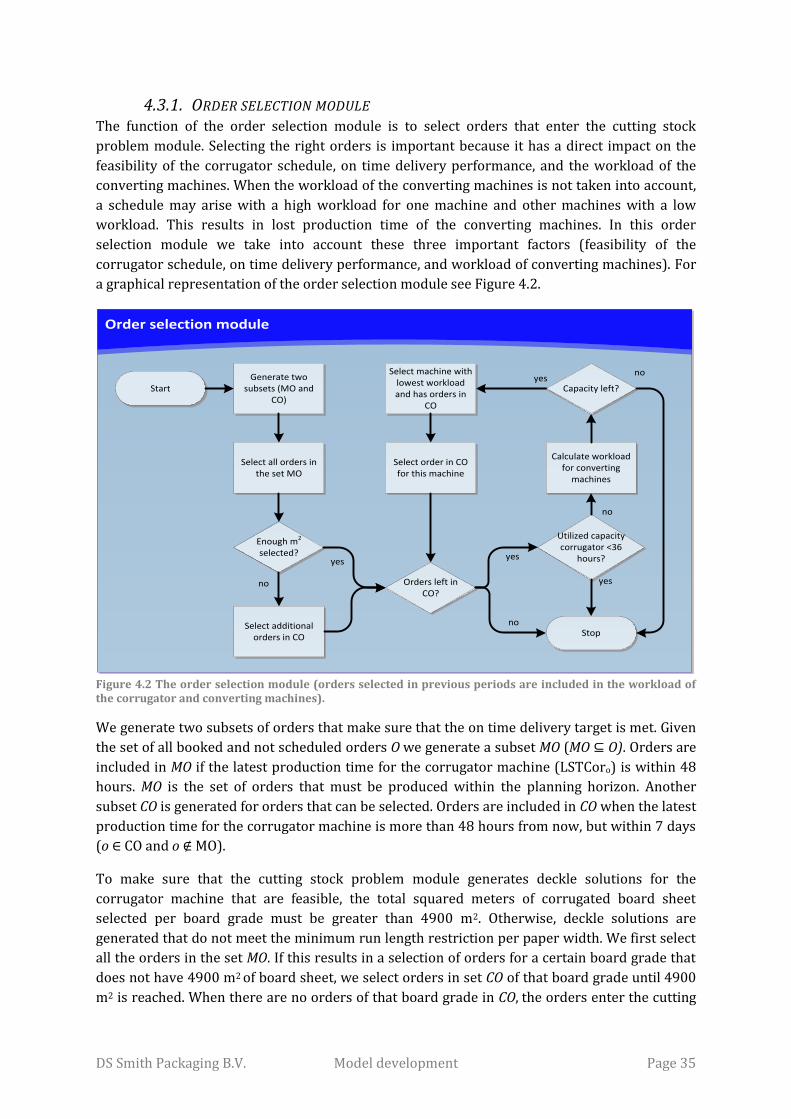
DS Smith Packaging B.V. Model development Page 35
4.3.1. ORDER SELECTION MODULE The function of the order selection module is to select orders that enter the cutting stock
problem module. Selecting the right orders is important because it has a direct impact on the
feasibility of the corrugator schedule, on time delivery performance, and the workload of the
converting machines. When the workload of the converting machines is not taken into account,
a schedule may arise with a high workload for one machine and other machines with a low
workload. This results in lost production time of the converting machines. In this order
selection module we take into account these three important factors (feasibility of the
corrugator schedule, on time delivery performance, and workload of converting machines). For
a graphical representation of the order selection module see Figure 4.2.
Figure 4.2 The order selection module (orders selected in previous periods are included in the workload of the corrugator and converting machines).
We generate two subsets of orders that make sure that the on time delivery target is met. Given
the set of all booked and not scheduled orders O we generate a subset MO (MO ⊆ O). Orders are
included in MO if the latest production time for the corrugator machine (LSTCoro) is within 48
hours. MO is the set of orders that must be produced within the planning horizon. Another
subset CO is generated for orders that can be selected. Orders are included in CO when the latest
production time for the corrugator machine is more than 48 hours from now, but within 7 days
(o ∈ CO and o ∉ MO).
To make sure that the cutting stock problem module generates deckle solutions for the
corrugator machine that are feasible, the total squared meters of corrugated board sheet
selected per board grade must be greater than 4900 m2. Otherwise, deckle solutions are
generated that do not meet the minimum run length restriction per paper width. We first select
all the orders in the set MO. If this results in a selection of orders for a certain board grade that
does not have 4900 m2 of board sheet, we select orders in set CO of that board grade until 4900
m2 is reached. When there are no orders of that board grade in CO, the orders enter the cutting
Order selection module
Generate two subsets (MO and
CO)Start
Select all orders in the set MO
Enough m2 selected?
Select additional orders in CO
Utilized capacity corrugator <36
hours?
Stop
Calculate workload for converting
machines
Select order in CO for this machine
Orders left in CO?
yes
yes
yes
no
no
no
Capacity left?
yes
no
Select machine with lowest workload and has orders in
CO

DS Smith Packaging B.V. Model development Page 36
stock problem module with a violation for the corrugator machine. This means that the
minimum run length restriction per paper width cannot be met and needs to be decreased in
order to find feasible deckle solutions.
Processing speeds for converting machines are known in advance. From this we calculate the
workload of an order for each converting machine (the workload is the sum of total processing
time and setup time). In order to make a schedule that results in a smooth and balanced
production process we need to balance the workload of the converting machines. We also have
information about the availability of a machine. This is measured in the total available days in
the planning horizon. We include the jobs that are accepted previous periods in the workload of
the converting machines. After that, we calculate the available time left for production for each
converting machine.
When enough m2 of corrugated board sheet is selected, we select the converting machine that
has the most available time left. For this selected machine we look for orders in the set CO that
may be processed on this machine and have a board grade that is already selected. The first
order based on latest production time for the corrugator machine is selected. The new
availability of the machines is calculated. Selecting orders is repeated until there are no orders
left, the corrugator machine is planned full for the next 36 hours, or all converting machines are
planned full for the next 36 hours.
4.3.2. CUTTING STOCK PROBLEM MODULE The cutting stock problem module is used to generate cutting patterns and solving the CSP in
order to generate deckle solutions. See Figure 4.3 for the graphical representation of the cutting
stock module. As mentioned in Chapter 3 we are dealing with a 1/V/D/R CSP. Upgrading of
board grades is not included in our model.
Figure 4.3 The cutting stock problem module. (mrlci = minimum run length per CI job, mrlw = minimum run length per paper width, both measured in meters)
It is preferable that each order is produced in the ordered board grade. Therefore, we solve the
CSP for each board grade separately, i.e., combining orders of different board grades is not
possible. We first select a board grade. Next, we generate all feasible cutting patterns for the
orders of the selected board grade. We initialize the minimum run length per CI job restriction
Cutting stock problem module
Select board grade
Start
Generate all feasible cutting patterns
mrlci = mrlci – 100mrlw = 2000
Feasible solution found?
Stop mrlw = mrlw - 100
mrlci ≤ mrlwSolve cutting stock
problem
All board grades solved?
yes
yes
yes
no
no
no
Store optimal solution
mrlci = 300mrlw = 2000

DS Smith Packaging B.V. Model development Page 37
(mrlci) and the minimum run length per paper width restriction (mrlw). After that, we use the
generated cutting patterns as parameters in the ILP model (see Appendix C for the complete ILP
model and pseudo code for generating the cutting patterns). If feasible solutions are found we
store the optimal one and select a new board grade. If all board grades are solved we stop the
cutting stock module. If no feasible solutions exist we decrease mrlw by 100 meters. If mrlw ≥
mrlci, we solve the ILP model. Otherwise the mrlci is decreased by 100 and mrlw is set to the
initial value. This means that we first look if no feasible solutions can be found due to the paper
width restriction. If this is not the case, we decrease the minimum run length per CI job
restriction.
GENERATING CUTTING PATTERNS In order to solve the ILP model we first need to generate the cutting patterns that are input
parameters for the model. We need to generate all feasible cutting patterns. A cutting pattern is
feasible when the trim loss is greater than or equal to the minimum trim loss. The minimum
trim loss constrained is used because the corrugated board on the sides is not of the right
quality and needs to be cut off. Moreover, the minimum trim loss is also needed because there
are tolerances on the paper reels and on the tool positioning that cut the corrugated board
sheets. There is a possibility to model the pattern generation in such way that we do not need
the minimum trim loss restriction. However, this is not preferred because the minimum trim
loss depends on the tolerances of the paper widths and on the accuracy of tool positioning. This
means that the minimum trim loss may vary for different board grades and may change if the
accuracy of the tool positioning improves. The model can be updated/ adapted easier when we
keep the minimum trim loss restriction in the model.
Another restriction is that the trim loss of the pattern must be smaller than or equal to the
maximum trim loss when two orders are in the cutting pattern. The maximum trim loss
constrained is needed because the waste retrieving system on the corrugator machine can only
handle trim waste up to the maximum trim loss. When one order is selected a side job can be
created. This means that the waste is not handled by the waste retrieving system of the
corrugator. Another important constraint is that the paper width that is used for the pattern
must be available for the given board grade. See Appendix B for the pseudo code of the
procedure that generates the cutting patterns. To generate all feasible cutting patterns we use
complete enumeration.
OBJECTIVE FUNCTION The objective function calculates the total trim loss produced in squared meters. This can be
calculated by multiplying the run length of pattern p (RLPp) with the trim loss of pattern p (tlp).
Using this objective function means that we find a deckle solution that minimizes the total
squared meters trim loss produced.
Min Z *p p
p
RLP tl
ADDITIONAL CONSTRAINTS The corrugator machine has some limitations. One of the limitations is that the run length of a CI
job must be at least 300 meters (mrlci). In order to incorporate this limitation we set up
constraint 4.2. For this we need an auxiliary binary variable, APp, which indicates if pattern p is
active {0 if inactive, 1 if active}, a pattern is active if it is used in a deckle solution (an active
pattern becomes a CI job). We need this variable because not all cutting patterns are active
(4.1)
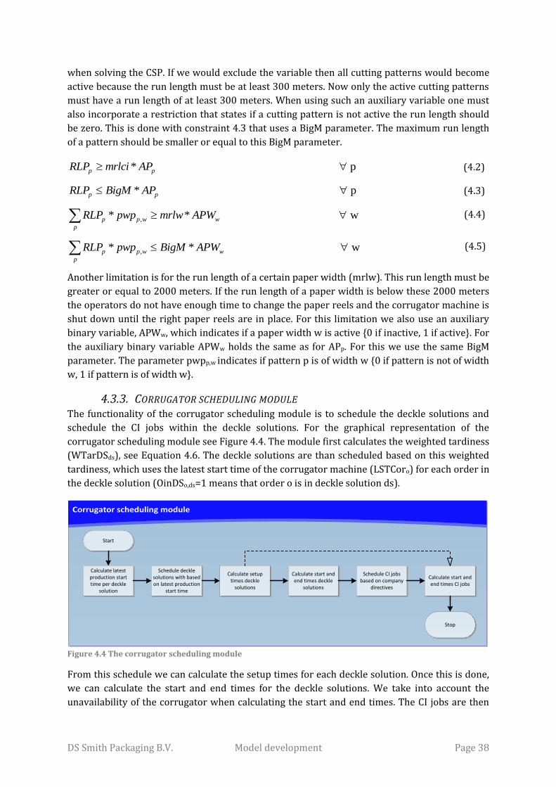
DS Smith Packaging B.V. Model development Page 38
when solving the CSP. If we would exclude the variable then all cutting patterns would become
active because the run length must be at least 300 meters. Now only the active cutting patterns
must have a run length of at least 300 meters. When using such an auxiliary variable one must
also incorporate a restriction that states if a cutting pattern is not active the run length should
be zero. This is done with constraint 4.3 that uses a BigM parameter. The maximum run length
of a pattern should be smaller or equal to this BigM parameter.
* pp pRLP mrlci AP
* pp pRLP BigM AP
,* * wp p w w
p
RLP pwp mrlw APW
,* * wp p w w
p
RLP pwp BigM APW
Another limitation is for the run length of a certain paper width (mrlw). This run length must be
greater or equal to 2000 meters. If the run length of a paper width is below these 2000 meters
the operators do not have enough time to change the paper reels and the corrugator machine is
shut down until the right paper reels are in place. For this limitation we also use an auxiliary
binary variable, APWw, which indicates if a paper width w is active {0 if inactive, 1 if active}. For
the auxiliary binary variable APWw holds the same as for APp. For this we use the same BigM
parameter. The parameter pwpp,w indicates if pattern p is of width w {0 if pattern is not of width
w, 1 if pattern is of width w}.
4.3.3. CORRUGATOR SCHEDULING MODULE The functionality of the corrugator scheduling module is to schedule the deckle solutions and
schedule the CI jobs within the deckle solutions. For the graphical representation of the
corrugator scheduling module see Figure 4.4. The module first calculates the weighted tardiness
(WTarDSds), see Equation 4.6. The deckle solutions are than scheduled based on this weighted
tardiness, which uses the latest start time of the corrugator machine (LSTCoro) for each order in
the deckle solution (OinDSo,ds=1 means that order o is in deckle solution ds).
Figure 4.4 The corrugator scheduling module
From this schedule we can calculate the setup times for each deckle solution. Once this is done,
we can calculate the start and end times for the deckle solutions. We take into account the
unavailability of the corrugator when calculating the start and end times. The CI jobs are then
Corrugator scheduling module
Calculate latest production start time per deckle
solution
Start
Schedule deckle solutions with based on latest production
start time
Stop
Calculate setup times deckle
solutions
Calculate start and end times deckle
solutions
Schedule CI jobs based on company
directives
Calculate start and end times CI jobs
(4.2)
(4.3)
(4.4)
(4.5)

DS Smith Packaging B.V. Model development Page 39
scheduled based on the company directives (see Section 2.5.2). When this schedule is also
determined we calculate the start and end times of the CI jobs, the setup times of the deckle
solutions are also used for the first CI job in a deckle solution. For an overview of the corrugator
scheduling module, see Appendix I.
,| 1
( ) dso ds
ds o
o OinDs
WTarDS LSTCor CurrentTime PlanningHorizon
CORRUGATOR SPEED In order to calculate the processing times of the CI jobs we
need to know the speed of the corrugator for a CI job.
Currently the ERP system of DS Smith calculates the speed as
follows: for each board grade Table 4.1 is filled in. The average
speed of a CI job is then determined by linear interpolation.
For example: if the run length of a CI job is 700 meters, then
the average speed of the corrugator is: 150 + (250-
150)*(700-500)/500 = 190 meters per minute. In this way
the average speed of the corrugator becomes dependent on the run length (RLCIci). Instead of
the linear interpolation method DS Smith is currently using, we propose to estimate the average
speed by using the cumulative exponential distribution (equation 4.7 and 4.8). According to the
production planners, the cumulative exponential distribution gives a better estimation of the
average corrugator speed (SCorci, bg) and requires less parameters. The cumulative exponential
distribution requires only the lambda (λbg) and the maximum speed (MaxSCbg) that are
dependent on the board grade (bg). The minimum speed (MinSC) is equal for all board grades.
See Figure 4.5 for an example of the average corrugator speed.
, * ,ci bg bg ci bgSCor F RLCI MaxSC MinSC MinSC
*
1, bg ciRLCIbg ciF e
Figure 4.5 Example average corrugator speed (MaxSCbg=300 ; λbg=0.00125)
Together with the production planners we decided that the lambda is equal for all board grades
and is estimated to be 0.00125. When necessary the lambda can be changed for each board
grades. The maximum speeds of all board grades are known and do not need to be evaluated.
Another variable to determine the speed is the length of each sheet within a CI job. The cutting
tools have a variable maximum speed, depending on the sheet length. The shorter the sheet
length, the lower the maximum speed of the cutting tools. The maximum speed of the cutting
0
50
100
150
200
250
300
350
0 200 400 600 800 1000 1200 1400 1600 1800 2000 2200 2400 2600 2800 3000
-->
SCo
r(R
LCI c
i, b
g)
(m
/min
)
--> RLCIci (m)
Run length Average speed (m/min)
0 60 500 150 1000 250 2000 300
(4.7)
(4.8)
Table 4.1 Example run speed corrugator machine
(4.6)

DS Smith Packaging B.V. Model development Page 40
tools (MaxTSci) is currently estimated by linear interpolation if the sheet length of an order that
is in the CI job (OinCIo,ci=1 means that order o is in CI job ci) is between the minimum sheet
length (480 mm) and the sheet length for which the maximum speed is reached (1200 mm). The
speed is equal to the maximum speed if the sheet length is equal or greater than 1200
millimeters. Producing sheets that are shorter than 480 mm is not possible. We choose to
estimate the maximum speed of the cutting tools the same as DS Smith. The minimum sheet
length is equal to 480 millimeters and the highest possible maximum speed is 300 meters per
minute. For the graphical representation of the maximum speed of the cutting tools see Figure
4.6 and for the calculation see Equation 4.9. To calculate the final estimated average speed
(ASCci,bg) we take the minimum of MaxTSci and SCorci,bg (See Equation 4.10).
| ( , ) 1
{ }
300 ; 100 200* 1200
min oo OinCI ci o
ci
sl
MaxTS min
, ,min ; ci bg cici bgASC SCor MaxTS
Figure 4.6 Example maximum speed cutting tools
SETUP TIMES CORRUGATOR Setup times are an important decision variable for the corrugator scheduling because the
corrugator machine is the bottleneck of the plant in Eerbeek. Setup times occur when there is a
board grade change on the corrugator machine. We determined the setup times together with
the operators of the corrugator machines. In most cases, the setup time is caused by a
corrugator roll change. For the different setup times dependent on the flute combination, see
Appendix E.
4.3.4. CONVERTING SCHEDULING MODULE The converting scheduling module constructs the schedule for the converting machines and
performs a load balancing procedure to improve the performance of the converting schedule.
The first step is to calculate the release time of each order for converting. This is determined by
the corrugator schedule, i.e., the time that stacks of order o are in the Pentek. After that the first
possible starting time for each job is determined based on the release time and in case of a
second converting job based on the finish time of precedence job. Also transportation and
drying time are taken into account in the first possible starting time calculation. The jobs are
scheduled based on this first possible starting time. After that, the performance of the schedule
is determined (tardiness of orders, waiting time of orders, and waiting on corrugator idle time).
0
50
100
150
200
250
300
350
48
0
56
0
64
0
72
0
80
0
88
0
96
0
10
40
11
20
12
00
12
80
13
60
14
40
15
20
16
00
16
80
17
60
18
40
19
20--
> M
axTS
(ci)
(m/m
in
--> min {slo} (mm)
(4.10)
(4.9)

DS Smith Packaging B.V. Model development Page 41
We use a load balancing heuristic to check if alternative converting machine routing would
improve the solution. For each job with waiting time alternative converting machine routes are
considered. The routing of these jobs is changed and the performance of the schedule is
evaluated. If the performance improves we accept the rerouting of the job. Otherwise the
rerouting is rejected. See Figure 4.7 for the graphical representation of the converting
scheduling module. We now elaborate on the transportation and drying time, precedence
relations, processing times, setup times, and the performance criteria.
Figure 4.7 The converting scheduling module consisting of two main parts: scheduling of converting jobs and the load balancing procedure.
TRANSPORTATION AND DRYING TIME It is important to take the transportation into account when calculating the first possible
starting time. Otherwise the starting times do not reflect the real situation. The transportation
times can be found in Appendix F. However, for some board grades the sheets of corrugated
board need to dry before the converting machines can process these sheets. This is required
because of quality issues. In case of drying time, not the transportation time but the total drying
time is taken into account for the first possible starting time, i.e., delay = max {transportation
time, drying time}.
PRECEDENCE RELATIONS Precedence relations exist for both a first and second converting job. The precedence relation
dictates that the first possible starting time of a converting job must be after the start of the first
CI job plus the delay, e.g., sheets for a converting job may be produced by multiple CI jobs. The
precedence relation for the second converting job is almost the same. The second job cannot
start before the start of the first converting job plus the transportation time.
Converting scheduling module
Load balancingSchedule converting
Determine release time based on
corrugator schedule
Start
Schedule jobs based on first available
starting time
Calculate start and end times jobs
Calculate initial performance
schedule
Determine first possible starting time based on precedence relations
and release time
J = 0
M = 1Machine m
possible for job j?
M = M + 1
M > number of converting machines
J = J+1
Job j has waiting time?
Change routing of job J to machine M
Schedule converting
Improvement in performance?
Accept new machine routing
and schedule
Reject new machine routing and
schedule
J > number of converting jobs?
End
no
yes
no
yes
yes no
no
yes
no
yes

DS Smith Packaging B.V. Model development Page 42
PROCESSING AND SETUP TIME Within the ERP system of DS Smith the historical machine processing speed per hour per order
is registered. This data is used to determine the processing speed per machine per order. This
data in combination with the planned quantity is used to calculate the total processing time. The
setup times for the converting jobs on each machine can be retrieved by the ERP system of DS
Smith. This data is used as input in our model.
PERFORMANCE CRITERIA In order to evaluate the performance of a schedule we need to calculate the performance
criteria. Important performance criteria for converting scheduling are the tardiness of orders,
waiting on corrugator (WOC) idle time and the waiting time of jobs. Tardiness is an important
criterion because there is a direct link with customer satisfaction. The other two performance
criteria are more internal criteria that have to do with efficiency.
4.3.5. PENTEK MODULE The Pentek module is a supporting module. The general model does not use the Pentek module
for (re)scheduling decisions. It is purely developed for the support of the production planners.
The Pentek consists of conveyors of seven different widths. We choose to model each width as
one long conveyor. So if there are ten conveyors with a width of two meters and length of
twenty meters we model it as one long conveyor of length 200 meters. We also modelled the
conveyors in front of the machines. The width of these conveyors is sufficient so we do not need
to take the width into account for these conveyors.
STACKS In order to calculate the fill rate of the conveyors we need to know how many stacks each CI job
produces per order (StaCIo,ci). The corrugated board sheets have a certain thickness (Tho) that is
determined by the board grade. We also need to know the stack height of each order (SHo). This
stack height is dependent on the sheet width. The smaller the sheet width, the lower the stack
height. The maximum stack height is 1800 mm when the width is equal or greater than 480 mm.
The minimum stack height is 750 mm when the width is equal to 260 mm (this is the minimum
sheet width). The stack height is determined by Equation 4.11. The number of stacks that each
CI job produces for an order is estimated by Equation 4.12 (NOinCIo,ci indicates how many times
order o is in CI job ci). From this we calculate the occupied meters in the Pentek by each CI job
(Equation 4.13) and by each order (Equation 4.14).
max 0;480 min 480;1800 1050*
260
o
o
swSH
o, ci
,
* *
*
o
o ci
o
ci
o
RLCI NOinCI ThStaCI
Ssl H
, , * slo ci o ci oStaCIMCI
,o o ci
ci
MCITMO
FILL RATE For the estimation of the fill rate of the Pentek we use fixed time intervals. We do this because
this simplifies the calculation and only has a limited effect on the reliability. To estimate the fill
rate of the Pentek we look at the number of stacks on each conveyor at each point in time. We
take a time interval of a quarter of an hour. This gives a reasonable estimation of the average fill
(4.11)
(4.12)
(4.13)
(4.14)
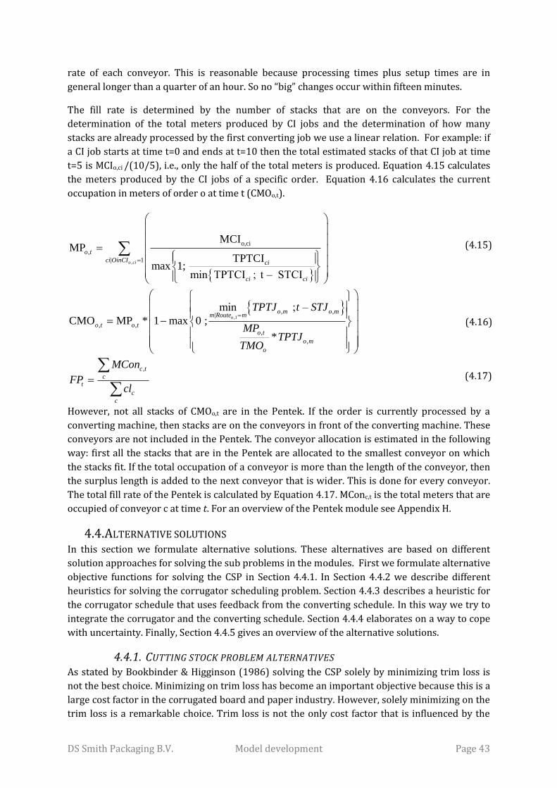
DS Smith Packaging B.V. Model development Page 43
rate of each conveyor. This is reasonable because processing times plus setup times are in
general longer than a quarter of an hour. So no “big” changes occur within fifteen minutes.
The fill rate is determined by the number of stacks that are on the conveyors. For the
determination of the total meters produced by CI jobs and the determination of how many
stacks are already processed by the first converting job we use a linear relation. For example: if
a CI job starts at time t=0 and ends at t=10 then the total estimated stacks of that CI job at time
t=5 is MCIo,ci /(10/5), i.e., only the half of the total meters is produced. Equation 4.15 calculates
the meters produced by the CI jobs of a specific order. Equation 4.16 calculates the current
occupation in meters of order o at time t (CMOo,t).
,
o,c
1
i
,
|
MCIMP
TPTCImax 1 ;
min TPTCI ; t – STCI
o cici OinCI ci
ci ci
o t
,1
, ,|
, ,
,
,
min ; –
CMO MP * 1 max 0 ;
*
o
o m o mm Route m
o t o t
o
o
t
o m
TPTJ t STJ
MPTPTJ
TMO
,c
t
t
c
c
c
F
MCon
cP
l
However, not all stacks of CMOo,t are in the Pentek. If the order is currently processed by a
converting machine, then stacks are on the conveyors in front of the converting machine. These
conveyors are not included in the Pentek. The conveyor allocation is estimated in the following
way: first all the stacks that are in the Pentek are allocated to the smallest conveyor on which
the stacks fit. If the total occupation of a conveyor is more than the length of the conveyor, then
the surplus length is added to the next conveyor that is wider. This is done for every conveyor.
The total fill rate of the Pentek is calculated by Equation 4.17. MConc,t is the total meters that are
occupied of conveyor c at time t. For an overview of the Pentek module see Appendix H.
4.4. ALTERNATIVE SOLUTIONS In this section we formulate alternative solutions. These alternatives are based on different
solution approaches for solving the sub problems in the modules. First we formulate alternative
objective functions for solving the CSP in Section 4.4.1. In Section 4.4.2 we describe different
heuristics for solving the corrugator scheduling problem. Section 4.4.3 describes a heuristic for
the corrugator schedule that uses feedback from the converting schedule. In this way we try to
integrate the corrugator and the converting schedule. Section 4.4.4 elaborates on a way to cope
with uncertainty. Finally, Section 4.4.5 gives an overview of the alternative solutions.
4.4.1. CUTTING STOCK PROBLEM ALTERNATIVES As stated by Bookbinder & Higginson (1986) solving the CSP solely by minimizing trim loss is
not the best choice. Minimizing on trim loss has become an important objective because this is a
large cost factor in the corrugated board and paper industry. However, solely minimizing on the
trim loss is a remarkable choice. Trim loss is not the only cost factor that is influenced by the
(4.15)
(4.16)
(4.17)

DS Smith Packaging B.V. Model development Page 44
CSP. Therefore we formulate three alternatives for solving the CSP. The first alternative uses
minimizing the total run length as objective. The second minimizes on production and trim loss
costs and the third alternative also takes into account costs associated with paper width and CI
job changes.
RUN LENGTH OBJECTIVE In the current situation the corrugator machine is the bottleneck of the plant in Eerbeek. The
machine is in production 24 hours a day, 5 days per week. This means that DS Smith uses the
full capacity of the corrugator machine. Since the total run length needed for a given set of
orders is dependent on the solution of the CSP, we can take this total run length into account.
Reducing the run length of a deckle solution means that we need to use less capacity of the
corrugator machine measured in meters. This results in a reduction of overtime needed or an
increase in available capacity for additional orders.
Min Z * 1100
p
p
p
tlRLP
We are not only using the run length in the objective function (see Equation 4.18). Only using
the run length could result in a deckle solution that has a minimum run length, but another
solution could exist with a minimum run length and also have a lower trim loss. We divide the
trim loss of a pattern by 100 in order to make the trim loss only important when the run length
of a solution is the same or very close to each other. The factor of 100 is a sufficient choice. The
trim loss of a pattern is between 32 and 200 mm (0.032 and 0.2 meter), so dividing it by 100
makes the run length be multiplied by a factor between 1.00032 and 1.002. The average run
length of a pattern is 2850 meters, so even if the trim loss is 200 mm the extra run length
accounted for is only 5.7 meters, which takes 1.7 seconds more production time. This is a
negligible difference.
COSTS MINIMIZATION Production cost of the corrugator machine (cc) is the other important cost factor in the
corrugated board industry. This can be expressed in cost per hour production. The baseline
costs are the personnel costs and the energy/utility costs. We can estimate the time needed to
produce a certain deckle solution with the average speed of the corrugator (asc). The average
speed of the corrugator is around 200 meters per minute. So if for example the run length for a
deckle solution is 10000 meters, the estimated production time is 50 minutes. We cannot use
the run length dependent average speeds. The objective function would not be linear anymore
and solving the CSP becomes a problem.
The exact cost for producing one hour on the corrugator machine is hard to define. Besides the
cost of energy and personnel, there are also depreciation costs of the machine, building, and
other fixed costs. Another cost factor that is open for debate is the cost of lost sales or
opportunity cost. When a deckle solution is chosen that has a long run length, there is no
capacity left to produce additional orders. This means that an opportunity is lost to make more
revenue and profit by producing additional orders. There is no data available about lost sales
and the profit margin, therefore it is debatable if we should take into account these cost. See
Equation 4.19 for the alternative objective function (cbgbg are the cost per m2 of corrugated
board of board grade bg).
(4.18)

DS Smith Packaging B.V. Model development Page 45
Min Z * *p p bg
p
ccRLP tl cbg
asc
COSTS MINIMIZATION: CI WASTE/TIME LOSS, PAPER WIDTH WASTE/TIME LOSS Trim loss is not the only factor in the CSP solution that results in waste. Also a CI job change and
a paper width change result in waste of corrugated board. On average, each CI job change
results in three meters waste of corrugated board. The total m2 of waste produced is dependent
on the gross width of the pattern (gwp). The average waste of corrugated board for a paper
width change is seven meters and the m2 of waste is dependent on the used paper width (w). A
CI job change results on average in a half minute of lost production time (twp) and a paper
width change results on average in five minutes of lost production time (tww). The objective
function becomes as stated by Equation 4.20
4.4.2. HEURISTICS FOR CORRUGATOR SCHEDULING In the general model we schedule the deckle solutions based on the latest start time of a deckle
solution. However, this does not result in a schedule that is preferable. These schedules have
much setup time and also have a bad performance based on tardiness. Therefore we formulate
three alternative heuristics. The first alternative is based on a 1-Opt heuristic, the second uses
the SA local search heuristic, and the third uses the AS construction heuristic. These heuristics
are based on a simultaneous optimization technique that uses a priori optimization. This means
that we formulate an objective function that takes into account two or more criteria.
OBJECTIVE FUNCTION CORRUGATOR SCHEDULING In order to evaluate the performance of a corrugator schedule we need to define the objective
function that is used by the different scheduling heuristics. The two important indicators are
tardiness of orders and the setup time of orders. At this stage we look at the tardiness of the
deckle solutions. Each order has a latest production time for the corrugator machine (LFTCoro)
and a deckle solution has a finishing time (FTDSds). The tardiness of a deckle solution is the
weighted sum of the tardiness of the orders within that deckle solution. Each customer has a
customer importance weight (CusImo). If it is a strategic customer, the weight is two, otherwise
the weight is one. See Equation 4.21 for the calculation of the total tardiness of the deckle
solutions (TTarDS).
,| 1
*o ds
o ds o
ds o OinDS
TTarDS LFTCor FTDS CusIm
50* ds
ds
Min Z TTarDS SetDS
It may seem redundant to use both tardiness and setup time. If setup time is decreased, less
time is needed for production and thus also tardiness is decreased and also vice versa. However,
there are situations where a schedule with more setup time may have a lower total tardiness.
Therefore we used both the tardiness and setup time for the objective function. The objective
function becomes as stated by Equation 4.22. Together with the production management at DS
Smith we set the importance of the setup time equal to 50 times the tardiness of the deckle
solutions. This means that reducing the setup time around 30 minutes is equal to reducing the
(4.20)
(4.19)
Min Z * * * * 3 * *7 *p
p w p p p p w bg
p w p w
RLPAP twp APW tww cc RLP tl gw AP APW w cbg
asc
(4.22)
(4.21)

DS Smith Packaging B.V. Model development Page 46
tardiness of the deckle solutions with one day. This gives an indication how important the
tardiness is compared to the setup time.
1-OPT HEURISTIC The 1-Opt heuristic is a local search heuristic that uses as starting point the schedule of the
previous period. The deckle solutions that are added in the current period are added
sequentially to the schedule. Then the start time is set. The first step of the heuristic is to select a
random deckle solution. This deckle solution is moved to another random place in the schedule.
This new schedule is evaluated based on the defined objective function. If the new schedule
improves the objective function then the new schedule is accepted. Otherwise the new schedule
is rejected. This is done until the elapsed time is greater or equal to the maximum time that is
available for the heuristic. See Figure 4.8 for the graphical representation of this heuristic.
Figure 4.8 Algorithm structure of the 1-Opt heuristic
SIMULATED ANNEALING (SA) HEURISTIC The SA algorithm is also a local search heuristic and starts with a corrugator schedule from the
previous period plus the new generated deckle solutions. The maximum time available for the
algorithm is converted to a start temperature, stopping temperature, interval temperature, and
max N (number of iterations per temperature). Then the current temperature is set to the start
temperature and n is set to zero.
Figure 4.9 Graph of the acceptance probability tested for different delta
1-Opt heuristic
Start
Set start time
Elapsed Time < MaxTimeSelect random deckle solution
Move to another random place in the
schedule
Calculate performance of the neighbor schedule
Neighbor objective value < best objective value
Best objective value = neighbor objective
value
Reject neighbor schedule
Calculate elapsed time
Stop
Generate starting schedule (using general model)
yesno
yes
no
Accept neighbor schedule
0
0.2
0.4
0.6
0.8
1
0 2 4 6 8 10 12 14 16 18 20 22 24 26 28
-> A
cce
pta
nce
pro
bab
ility
-> Temperature Delta=0.25 Delta=0.5 Delta=1 Delta=1.5 Delta=2 Delta=3
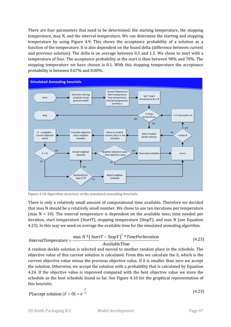
DS Smith Packaging B.V. Model development Page 47
There are four parameters that need to be determined: the starting temperature, the stopping
temperature, max N, and the interval temperature. We can determine the starting and stopping
temperature by using Figure 4.9. This shows the acceptance probability of a solution as a
function of the temperature. It is also dependent on the found delta (difference between current
and previous solution). The delta is on average between 0.5 and 1.5. We chose to start with a
temperature of four. The acceptance probability at the start is then between 90% and 70%. The
stopping temperature we have chosen is 0.1. With this stopping temperature the acceptance
probability is between 0.67% and 0.00%.
Figure 4.10 Algorithm structure of the simulated annealing heuristic
There is only a relatively small amount of computational time available. Therefore we decided
that max N should be a relatively small number. We chose to use ten iterations per temperature
(max N = 10). The interval temperature is dependent on the available time, time needed per
iteration, start temperature (StartT), stopping temperature (StopT), and max N (see Equation
4.23). In this way we need on average the available time for the simulated annealing algorithm.
2
max * *N StartT StopT TimePerIterationIntervalTemperature
AvailableTime
A random deckle solution is selected and moved to another random place in the schedule. The
objective value of this current solution is calculated. From this we calculate the δ, which is the
current objective value minus the previous objective value. If δ is smaller than zero we accept
the solution. Otherwise, we accept the solution with a probability that is calculated by Equation
4.24. If the objective value is improved compared with the best objective value we store the
schedule as the best schedule found so far. See Figure 4.10 for the graphical representation of
this heuristic.
{accept solution | 0} TP e
Simulated Annealing heuristic
Start
T≤ Stop temperature
Select random deckle solution
Move to another random place in the
schedule
Calculate objective value neighbor
schedule
Random(0,1)< Exp(-δ /T)
Store best schedule
Stop
Generate starting schedule (using general model)
yes
no
yes
no
Convert Maxtime to Start temperature, Stop temperature,
interval temperature, and Max n
Set T=start temperature & n=0
δ = (neighbor-current objective
value)
δ ≤ 0Accept neighbor
scheduleNeighbor objective value
< best objective value
Reject neighbor schedule
n=n+1
n=Max N
T=T-interval & n=0
yes
no
no
yes
yes
no
(4.23)
(4.23)

DS Smith Packaging B.V. Model development Page 48
ADAPTIVE SEARCH (AS) HEURISTIC The AS algorithm is a construction heuristic that sequentially adds deckle solutions to a
schedule. The performance of these schedules is evaluated each iteration of the algorithm. If the
objective function is better than the best solution then store the current schedule as the best
schedule. The current schedule is emptied and a new schedule is constructed via the
construction heuristic. See Figure 4.11 for the graphical representation of this AS algorithm.
Constructing new solutions is based on the priorities of the deckle solutions. The AS algorithm
uses priorities based on the tardiness of orders and setup time of a deckle solution. In order to
calculate the setup time of a deckle solution we need to store the flute combination of the
previous deckle solution. We construct a subset ADS of the to schedule deckle solutions (SD).
The deckle solutions in this subset are not yet scheduled by the AS Algorithm and do not have a
fixed sequence. The setup time (SetASds) is estimated by Equation 4.25. The tardiness of deckle
solutions (TTarASds) is based on the difference between the current start time (CSTAS) and the
latest start time of an order for the corrugator machine that is in deckle solution ds.
Figure 4.11 Algorithm structure of the adaptive search heuristic
Pr , dsds evFC FCSetAS SetFC ds ADS
,|OinDS 1
max{0; STAS LSTCor } o ds
o
o
dsTTarAS C ds ADS
The calculation of the priority (φds) is based on the objective function for the corrugator
schedule. This priority uses an estimation of the setup time and finishing time. From these
priorities we can calculate the regret (Rds) and probabilities (Pds) that a deckle solution is
chosen as next deckle solution in the schedule. For the probability calculation we use α=10. The
estimation may be unreliable in case of unavailability of the corrugator machine. However,
taking into account the unavailability would require more computation time. We use the
estimation because we can then investigate more solutions.
50*SetAS dds s dsTTarAS ds ADS
Adaptive Search heuristic
Start Set start time
Elapsed Time < maxtime
ASD empty
Calculate φsd, Rsd,
and Psd for all sd
in set ADS
Randomly select a deckle solution
based Psd
Assign selected sd to the schedule
Calculate performance
current scheduleImprovement
Store current schedule as best
schedule
Empty current solution
Stop
yes
no
yes
no
no
Initialize set ASD
Set sequence deckles equal to best sequence
Update CurrentStartTimeAS
Remove selected sd from set ASD
Calculate elapsed time
yes
(4.25)
(4.26)
(4.27)

DS Smith Packaging B.V. Model development Page 49
min ds ds dsds ADS
R ds ADS
( 1)
( 1)
ds
ds
ds
ds ADS
RP ds ADS
R
The elapsed time is calculated after each iteration of the AS heuristic. If there is time left
(elapsed time < maxtime) a new iteration of the AS algorithm is started. Otherwise the sequence
of the deckle solutions is set to the best sequence found by the AS algorithm.
We determine the alpha by running the heuristic for four different situations. With each
situation we tested what the average objective value, minimum objective value, maximum
objective value, and the standard deviation was for different alpha (α = 10, 15,..., 50, 55). In
three of the four situations we found the minimum objective value with an alpha of 35. Also the
differences in average, maximum, standard deviation with using another alpha are acceptable.
Therefore we use an alpha of 35 for our model. See Appendix K for the results of the four
situations.
4.4.3. INTEGRATING CORRUGATOR AND CONVERTING SCHEDULING Finding a good corrugator schedule does not necessarily mean that we also find a good
converting schedule. This is because the latest start time does not take into account waiting time
at the converting machines. However, in most cases the jobs have waiting time and this can
result in tardiness of orders. Another important point is that we do not to take into account the
workload when scheduling the corrugator machine. Because of this, WOC idle time can occur at
one or more of the converting machines. To make sure the corrugator schedule is not conflicting
with the converting machine we integrate the two schedules. We do this by using the
lexicographical optimization technique. This means that we first optimize based on one
criterion and after that we optimize based on another criterion. We use a restriction that states
that the objective of the first optimization should stay the same or should improve (if the
optimal is not found). We added this restriction because tardiness of orders is more important
than WOC idle time.
We do this by checking which deckle solution produces most tardy orders. Then we evaluate a
new schedule where this deckle solution is produced earlier in the schedule. If this results in a
decrease in the number of tardy orders we accept this new solution. Otherwise we reject the
solution. This is done for an amount of time that can be defined in the model.
After we optimized based on tardiness, we optimize based on WOC idle time. We calculate the
WOC idle time in front of each job on a converting machine. For each deckle solution the WOC
idle times of the orders in that deckle solution are summed up. The deckle solution with the
most total WOC idle time is then produced at another time in the schedule. If this results in a
decrease in the total WOC idle time and the number of tardy orders is the same or less we
accept the new schedules. Otherwise we reject the new schedules. This is done for a certain
amount of time that is defined for each alternative.
4.4.4. PROACTIVELY COPING WITH UNCERTAINTY We deal with a production process that has many uncertainties, e.g., machines may break down,
unavailability of personnel, lower than expected processing speeds, etcetera. Therefore it is
important to take into account uncertainty proactively instead of reactively what is currently
(4.28)
(4.29)

DS Smith Packaging B.V. Model development Page 50
done. In Chapter 3 we discussed the five approaches for coping with uncertainty. The only one
that is interesting for DS Smith is the proactive robust scheduling approach where durations are
increased or idle time is inserted. Stochastic and fuzzy scheduling are not applicable for DS
Smith because of the unavailability of probability functions and the high number of jobs that are
performed each day.
Gao (1995) uses the mean time between failures and the mean repair time to determine the
average duration of a job on a certain machine (called temporal protection). See Equation 4.30,
where P is the estimated processing time, F is the mean time between failures and D is the mean
repair time.
* *(1 )P D
Expected duration P D PF F
, , , ( m)* o,o m o m o m mTPTJ PTJ SetJ Factor
However, we do not have any information of the mean time between failures and the mean
repair time. We do have information of all stops of the machines that took longer than one
minute. But this information is not always reliable and there are also stops that may be a result
of the schedule, e.g., WOC, Waiting on full Pentek, idle times, etcetera. We can see that using the
mean time between failures and the mean time to repair is nothing more than multiplying the
estimated processing time with some factor >1. We use this factor for the calculation of the
expected total production time (TPTJo,m) for our model (PTJo,m is the processing time of order o
on machine m and SetJo,m is the setup time of order o at machine m) (See Equation 4.31). The
only thing we need to do is setting a factor for each converting machine (Factorm).
In order to determine these factors we asked for the opinion of the production and expedition
planners. They mention that the scheduled finishing times increase on average 2-3 hours for the
converting machines looking at a range of 24 hours. Therefore we propose to use a factor for
each machine of 1.1. This would imply that at each machine there are on average 2.4 hours of
unexpected events each day. This is a rough estimation of the average delay due to unexpected
events. Therefore, this factor needs to be evaluated and updated in order to improve the
robustness of a schedule. We do not use temporal protection for the corrugator machine. This
machine is more reliable than the converting machines and has a lower number of stops with in
total less stopping time per day. The increase in scheduled total production time does not affect
the first possible starting times of jobs on the same machine. So if no unexpected events occur,
then preceding jobs on that machine can start earlier until they reach their first possible starting
time. In this way we delete the buffer for unexpected events of the already finished job. This is
important because otherwise this could result in an accumulation of buffers and may result in
idle time of machines.
4.4.5. OVERVIEW ALTERNATIVE SOLUTIONS The objective of this research is to give an integrated solution. Therefore we combine the
alternatives formulated in the previous subsections. The order selection process is the same for
all alternatives. Then for the CSP we are going to test the current objective (trim loss) and a new
objective. In Chapter 5 the different alternative objective functions are discussed and evaluated
and the best alternative objective is chosen. After the CSP we are going to generate a corrugator
schedule with the 1-Opt heuristic, AS algorithm, SA algorithm, and according to the general
corrugator module. Finally all the jobs are first scheduled according to the FIFO rule and a load
(4.30)
(4.31)

DS Smith Packaging B.V. Model development Page 51
balancing iteration is performed. After that, we run the integrated corrugator and converting
scheduling procedure. We test in total eight alternatives (see Figure 4.12).
Figure 4.12 Overview of the alternative solutions
4.5. CONCLUSIONS In this chapter we formulated the general model. This model consists of an order selection
module, a cutting stock module, a corrugator scheduling module, a converting module, and a
Pentek module. We formulated alternatives for the cutting stock module, corrugator module,
and we formulated an alternative that integrates corrugator and converting scheduling. The
alternatives for the CSP are different in the objective function of the ILP model. The current
objective function is to minimize on trim loss. The alternative objective functions are
minimizing the total run length, minimizing on production costs, and minimizing on production
costs including waste and time loss of changes (CI and paper width). The alternatives for the
corrugator scheduling are two local search methods: a 1-Opt heuristic and a simulated
annealing heuristic, and an adaptive search heuristic that is a construction heuristic. Finally we
integrate the corrugator and converting scheduling by making decisions for rescheduling of the
corrugator schedule that are dependent on the converting schedule. We evaluate the
alternatives in Chapter 5.
Alternatives
Alternative 1 Alternative 2 Alternative 3 Alternative 5 Alternative 6 Alternative 7 Alternative 4 Alternative 8
End
peri
odO
rder
Sel
ecti
on
mod
ule
CSP
mod
ule
Cor
ruga
tor
mod
ule
Con
vert
ing
mod
ule
Star
t pe
riod
Cor
ruga
tor
and
Con
vert
ing
Mod
ule
Order Selection
CSP (Trim loss) CSP (new)
1-Opt heuristic
Adaptive Search
Simulated Annealing
1- Opt heuristic
Adaptive Search
Simulated Annealing
Integrated corrugator and converting scheduling
Start Alternative 1 Start Alternative 2
End Alternative 1 End Alternative 2 End Alternative 3 End Alternative 4 End Alternative 5 End Alternative 6 End Alternative 7 End Alternative 8
Schedule FIFO and perform Load balancing
Basic module
Basic module
Start Alternative 3 Start Alternative 4 Start Alternative 5 Start Alternative 6 Start Alternative 7 Start Alternative 8

DS Smith Packaging B.V. Model development Page 52

DS Smith Packaging B.V. Evaluating alternative solutions Page 53
5. EVALUATING ALTERNATIVE SOLUTIONS In Chapter 4 we formulated the general model, alternative objective functions for solving the
cutting stock problem, and formulated alternative solutions. This chapter answers the fourth
research question: “What is the best alternative for the cutting stock and scheduling problem at
DS Smith?”
In this chapter we evaluate the alternative solutions. In Section 5.1 we evaluate the alternative
CSP objective functions. Section 5.2 evaluates the alternative solutions and selects the best
solution. Section 5.3 elaborates on the differences of the selected solution with the current
situation and how this selected solution may be used. Finally in Section 5.4 we give conclusions.
5.1. ALTERNATIVE CUTTING STOCK PROBLEM OBJECTIVES In this section we evaluate the alternative CSP objective functions and select the best objective
function.
5.1.1. EXPERIMENTAL DESIGN In Chapter 4 we formulated alternative objective functions for the CSP. These alternative
objective functions are evaluated using the orders with a due date between 1-1-2014 and 30-4-
2014. The first week is used for the warm-up period and the last week is used as cool-down
period. For the order selection we use a simplified version of the order selection module (see
Section 4.3.1.). We use a simplified version because in this way the selected orders are the same
within each alternative.
We simplify the order selection by using a rolling horizon of 12 hours. During this horizon
350000 m2 of corrugated board can be selected. We use the same sets of orders as in the
general model, i.e., a set of orders that must be selected and a set of orders that can be selected.
All the orders in MO are selected and orders in the set CO are added when not enough m2 is
selected for a specific board grade. If there is still capacity left then orders in the set CO are
added until the capacity of the corrugator is filled. After the order selection the CSP is solved
and the horizon will be shifted 12 hours. This process is repeated until 30-4-2014 is reached.
Because the order selection is the same for all alternatives, the deckle solutions contain the
same orders. This means that we can perform a pairwise T-test for the deckle solutions. For the
CI jobs we cannot perform a pairwise T-test because they are not comparable, i.e., deckle
solutions may have a different number of CI jobs of different length and use different paper
widths. We are evaluating the alternatives based on: trim loss (Euro and m2), total run length,
number of paper widths used, number of CI jobs used, and total costs based. We exclude the
alternative where the waste and time loss of paper width and CI job changes is taken into
account in the objective function. Solving the ILP with this objective function takes too much
time. Moreover, the differences with the other cost objective function are small. We perform a
sensitivity analysis on the production cost per hour and the speed of the corrugator machine
(200 m/min and 250 m/min). In order perform the sensitivity analysis we defined 20
alternatives for the cost objective function. For the minimum trim loss objective function and
minimum run length objective function we only defined one alternative, i.e., the cost and speed
of the corrugator machine do not have an impact on the found deckle solutions by these
objective functions. For an overview of the 22 alternatives see Appendix J.

DS Smith Packaging B.V. Evaluating alternative solutions Page 54
5.1.2. RESULTS The results of the experiments are shown in Table 5.1 and Table 5.2. In these tables we outlined
what the change in percentage was between alternative 1 (the current objective function) and
the other alternatives. All differences in total run length, number of widths used, the baseline
costs, trim loss cost and m2 are significant with 97.5% certainty (tested with the pairwise t-test).
The differences in number of CI jobs in a deckle solution are only significant between alternative
1 and 2. However, this change is relatively small, i.e., a reduction of 0.037 CI job per deckle
solution (-0.94%).
Alternative Total Run length (m)
% Change
# Widths % Change
# CI jobs % Change
1 (trim loss) 16460774 0.00% 1.632 0.00% 3.805 0.00%
2 (run length) 15996689 -2.82% 1.373 -15.86% 3.768 -0.98%
3 (cost 200; speed 200) 16342967 -0.72% 1.590 -2.57% 3.805 0.00%
4 (cost 400; speed 200) 16264669 -1.19% 1.562 -4.26% 3.799 -0.15%
5 (cost 600; speed 200) 16214399 -1.50% 1.539 -5.70% 3.795 -0.28%
6 (cost 800; speed 200) 16156073 -1.85% 1.514 -7.19% 3.792 -0.34%
7 (cost 1000; speed 200) 16133379 -1.99% 1.503 -7.87% 3.797 -0.22%
8 (cost 1200; speed 200) 16106124 -2.15% 1.495 -8.39% 3.803 -0.05%
9 (cost 1400; speed 200) 16091700 -2.24% 1.490 -8.67% 3.811 0.14%
10 (cost 1600; speed 200) 16080277 -2.31% 1.479 -9.36% 3.793 -0.33%
11 (cost 1800; speed 200) 16067998 -2.39% 1.473 -9.72% 3.810 0.12%
12 (cost 2000; speed 200) 16062542 -2.42% 1.463 -10.32% 3.800 -0.14%
13 (cost 200; speed 250) 16363005 -0.59% 1.596 -2.17% 3.797 -0.22%
14 (cost 400; speed 250) 16290827 -1.03% 1.570 -3.78% 3.804 -0.03%
15 (cost 600; speed 250) 16246490 -1.30% 1.553 -4.82% 3.805 0.00%
16 (cost 800; speed 250) 16206591 -1.54% 1.530 -6.22% 3.792 -0.34%
17 (cost 1000; speed 250) 16156073 -1.85% 1.514 -7.19% 3.792 -0.34%
18 (cost 1200; speed 250) 16136804 -1.97% 1.506 -7.71% 3.799 -0.17%
19 (cost 1400; speed 250) 16110752 -2.13% 1.495 -8.39% 3.803 -0.07%
20 (cost 1600; speed 250) 16097722 -2.21% 1.491 -8.59% 3.799 -0.17%
21 (cost 1800; speed 250) 16090285 -2.25% 1.489 -8.76% 3.807 0.03%
22 (cost 2000; speed 250) 16080277 -2.31% 1.479 -9.36% 3.793 -0.33% Table 5.1 the total run length, the number of widths used, and the number of CI jobs used for each alternative. The italic grey numbers are the non-significant differences.
From these results we conclude that taking into account the cost of the corrugator results in a
reduction in total run length. The higher the costs, the higher the reduction in total run length.
The same holds for the number of widths used. Both reductions have a positive effect on the
available capacity of the corrugator machine. The shorter the total run length needed, the more
capacity is left for additional orders or a reduction in overtime needed. Next to this, reducing
the number of paper widths used in a deckle solution results in a reduction of changeover time
and changeover waste. The maximum reduction in run length is -2.82% since this is the
minimum run length option. Also the minimum run length option (alternative 2) has the highest
reduction in number of widths used (-15.86%). This can be explained by the fact that in order to
reduce the total run length, we need to maximize the utilization of the width of the corrugator
machine.

DS Smith Packaging B.V. Evaluating alternative solutions Page 55
However, minimizing on total run length has a high impact on the trim loss. The total trim loss
measured in m2 increases with 9.17% and the trim loss measured in cost increases with 7.84%.
This is much more than the increase in trim loss when minimizing on cost. Taking €2000 as
production cost per hour results in an increase in trim loss in m2 of 4.05% and increase in trim
loss cost of 3.36%. This is less than the half of the percentage change of alternative 2, while the
extra reduction in run length by alternative 2 is only 0.4% (2.82% instead of 2.42%). Another
interesting result is that the increase in square meters trim loss is higher than the increase in
trim loss cost. An explanation may be that there are large differences in cost per square meter
per board grade.
Alternative Baseline Costs
% Change
Trim Loss m 2
% Change
Trim Loss costs
% Change
1 (trim loss) € 963.792 0.00% 1831333 0% € 528.939 0.00%
2 (run length) € 992.393 2.97% 1999192 9.17% € 570.406 7.84%
3 (cost 200; speed 200) € 961.659 -0.22% 1835676 0.24% € 529.876 0.18%
4 (cost 400; speed 200) € 961.437 -0.24% 1843789 0.68% € 531.715 0.52%
5 (cost 600; speed 200) € 962.159 -0.17% 1852965 1.18% € 533.807 0.92%
6 (cost 800; speed 200) € 963.852 0.01% 1865854 1.89% € 537.081 1.54%
7 (cost 1000; speed 200) € 964.907 0.12% 1872929 2.27% € 538.745 1.85%
8 (cost 1200; speed 200) € 966.620 0.29% 1882578 2.80% € 541.143 2.31%
9 (cost 1400; speed 200) € 967.787 0.41% 1888413 3.12% € 542.667 2.60%
10 (cost 1600; speed 200) € 968.860 0.53% 1894589 3.45% € 544.117 2.87%
11 (cost 1800; speed 200) € 970.314 0.68% 1901707 3.84% € 545.865 3.20%
12 (cost 2000; speed 200) € 970.957 0.74% 1905436 4.05% € 546.725 3.36%
13 (cost 200; speed 250) € 961.854 -0.20% 1834255 0.16% € 529.571 0.12%
14 (cost 400; speed 250) € 961.383 -0.25% 1840591 0.51% € 530.975 0.38%
15 (cost 600; speed 250) € 961.610 -0.23% 1846404 0.82% € 532.374 0.65%
16 (cost 800; speed 250) € 962.308 -0.15% 1854736 1.28% € 534.210 1.00%
17 (cost 1000; speed 250) € 963.852 0.01% 1865854 1.89% € 537.081 1.54%
18 (cost 1200; speed 250) € 964.727 0.10% 1871644 2.20% € 538.465 1.80%
19 (cost 1400; speed 250) € 966.266 0.26% 1880805 2.70% € 540.695 2.22%
20 (cost 1600; speed 250) € 967.244 0.36% 1885620 2.96% € 541.998 2.47%
21 (cost 1800; speed 250) € 967.907 0.43% 1889229 3.16% € 542.835 2.63%
22 (cost 2000; speed 250) € 968.860 0.53% 1894589 3.45% € 544.117 2.87% Table 5.2 the total baseline cost, trim loss produced measured in m2, and trim loss produced measured in cost for each alternative
The total baseline cost includes costs that are certainly made (production cost per hour, board
grade cost, and cost of paper width and CI job changes). When calculating with €200, €400, or
€600 production cost per hour we get a reduction in total baseline cost. Using production cost
per hour that are higher than €600 results in an increase in total baseline cost. However, this
increase is only 0.77% when using €2000 as production cost per hour.
We also calculate the differences in total cost when taking into account different baseline cost
for the corrugator machine. We exclude the cost of paper width and CI job changes because the
differences in total costs caused by these costs are only small. We include the cost of lost sales in
the baseline cost. Given that the capacity of the corrugator machine is 600000 of m2 corrugated

DS Smith Packaging B.V. Evaluating alternative solutions Page 56
board per day. We estimate the cost of lost sales by Equation 5.1. So if the profit margin per m2
is €0.01, the cost of lost sales per hour production is €250. Together with the management of DS
Smith we decide that the profit margin per m2 of corrugated board sheet is around € . confidential
This means that we have around € of lost sales per hour production. The total confidential
production cost per hour are then around € euros. confidential
2600000profit margin per hour production *profit margin per m
24
See Figure 5.1 for the differences in cost with the minimum trim loss alternative for different
production cost per hour. An important observation is that when the production costs per hour
are €1100 or more there is always a cost decrease.
Figure 5.1 Cost difference with minimum trim loss alternative for different production cost per hour
5.1.3. CONCLUSIONS From the results of the experiments we conclude the following:
Using the trim loss objective is only the best option when the production cost per hour
of the corrugator machine is less than €100 per hour.
Using the run length objective is never the best option looking at a range of the
production cost per hour of the corrugator machine between €0 euro and €2000 per
hour.
The solutions found by using the cost minimization objective are dependent on the costs
per hour production of the corrugator machine.
Using the cost minimization objective with cost of the corrugator of €0 results in the
same solutions as by using the trim loss objective.
Using the cost minimization objective with production cost of the corrugator machine
that is near to infinity is the same as using the minimum run length objective.
The higher the average speed of the corrugator, the smaller the effect of the production
cost per hour of the corrugator machine.
The cost minimization objective is a flexible objective. The same solutions as with the
trim loss and run length objective can be obtained by changing the production cost per
hour of the corrugator machine.
€(55,000)
€(45,000)
€(35,000)
€(25,000)
€(15,000)
€(5,000)
€5,000
€15,000
€25,000
€35,000
€45,000
€ 0
€ 1
00
€ 2
00
€ 3
00
€ 4
00
€ 5
00
€ 6
00
€ 7
00
€ 8
00
€ 9
00
€ 1
,00
0
€ 1
,10
0
€ 1
,20
0
€ 1
,30
0
€ 1
,40
0
€ 1
,50
0
€ 1
,60
0
€ 1
,70
0
€ 1
,80
0
€ 1
,90
0
€ 2
,00
0
Co
st d
iffe
ren
ce w
ith
min
imu
m t
rim
loss
al
tern
ativ
e
Production cost per hour for the corrugator machine Minimal run length Minimal cost (200 Euro)Minimal cost (400 Euro) Minimal cost (1000 Euro)
(5.1)

DS Smith Packaging B.V. Evaluating alternative solutions Page 57
We propose the cost objective for solving the CSP at DS Smith. Given that the minimum
production costs per hour of the corrugator machine are at least € per hour, we confidential
conclude that using the minimum trim loss objective is never the best choice. Using the
minimum run length objective is also not a good choice. The same solution is found as when the
production costs per hour of the corrugator machine are near to infinity. We propose to use €
production costs per hour. The minimum costs are at least € and we decided confidential confidential
that the costs of lost sales are around € per m2 of corrugated board sheet; this is confidential
around € per hour production. This objective function gives good results even if this confidential
estimation is not correct. The cost deviation would only be 0.06% when the production costs
per hour would be €1600 and 0.07% when the production costs would be €600. Therefore we
conclude that using € is a robust choice for solving the CSP. confidential
5.2. ALTERNATIVE INTEGRATED SOLUTIONS The cutting stock problem module is only one module of the whole solution. Therefore we also
need to test several solutions that combine the alternatives of the modules.
5.2.1. PERFORMANCE MEASUREMENT In Chapter 3 we discussed performance measurement for production scheduling. Bandinelli et
al. (2005) propose a framework based on three domains: the effectiveness, robustness, and
flexibility domain. However, for the evaluation of the alternative solutions only the effectiveness
is important. The alternatives score the same on robustness and flexibility, so there is no need
to include this. The effectiveness domain measures the effectiveness of a schedule. So this
measures the performance under a steady-state situation. For the evaluation of the alternative
solutions we are using the following criteria:
TARDINESS We split up the tardiness criteria in average tardiness, total tardy orders, and % tardy orders.
This is not the average tardiness of all orders, but the average tardiness of tardy orders. It is
important to know how much the tardiness of an order is on average. If there are many tardy
orders that are only one hour finished too late it is less bad than having less tardy orders that
are one day finished too late. Orders that are a few hours finished too late can still be delivered
on time in most cases. We also need to know how many orders are tardy and what percentage of
the orders is tardy.
Average tardiness
Total tardy orders
Percentage tardy orders
EARLINESS The earliness measures how much time the order is finished before the delivery date. If an order
is delivered too late, the earliness becomes zero. We use the average earliness of orders because
having a high average earliness means having many finished products. This costs capital
investment and an increase in warehouse capacity is needed. Therefore it is preferable to
produce JIT and keep the average earliness low.
Average earliness

DS Smith Packaging B.V. Evaluating alternative solutions Page 58
TRIM LOSS Trim loss is currently the only factor for solving the CSP. We defined another objective function
that also takes into account the production costs. Therefore it is necessary to analyze what the
effect on the average trim loss is when we use another objective function.
Average trim loss %
OUTPUT OF THE CORRUGATOR MACHINE The output of the corrugator machine is used for the performance measurement since the
corrugator machine is the bottleneck of the plant of DS Smith. We expect that the alternatives
that use the cost objective function have a lower average run length per deckle solution. This
means that less capacity is needed. However, a decrease in average run length per CI job results
in lower average speeds (see Section 4.3.3).
Total run length
Total square meters produced
Average run length of an deckle solution
Average run length per CI job
WAITING TIME AND FILL RATE OF THE PENTEK Currently the Pentek causes problems when the fill rate becomes too high (>75%). Therefore it
is important to know the average and maximum fill rate of alternative solutions. Moreover, the
average waiting time per order is also important because high average waiting time probably
results in a high average fill rate.
Average waiting time per order
Average fill rate
Maximum fill rate
WOC IDLE TIME The WOC idle time needs to be minimized in order to produce efficiently. Therefore we need to
know the average WOC idle time before an order and the total WOC idle time per machine.
Average WOC idle time before an order
Total WOC idle time per machine
SIMPLICITY The last criterion is about the simplicity of the solution. Simple solutions are easier to
implement and understand. This increases the probability of a successful implementation.
5.2.2. EXPERIMENTAL DESIGN The eight alternatives formulated in Section 4.4 needs evaluation. We do this by first creating an
initial situation (warm-up period). This is done by running the model for two weeks by the
general model. After that we solve the next two weeks using each alternative. In this way we can
compare the alternatives. The warm-up period is from 17-3-2014 until 30-3-2014. Then we run
the model for the next twee weeks with each alternative, so until the current date is 14-4-2014.
We do not need a cool-down period because the data of jobs that are finished before 14-4-2014
are not changing anymore. We analyzed our results with jobs (corrugator and converting) that
started after 30-3-2014 and finished before 14-4-2014. We use a scheduling horizon of one and
a half days (36 hours) and a rolling horizon of half a day (12 hours).

DS Smith Packaging B.V. Evaluating alternative solutions Page 59
For the unavailability of machines we use the actual predictable unavailability for each machine.
The last minute personnel unavailability, corrective maintenance, and other stop causes are
included in the stops for each machine. We use historical data about the stops to estimate the
results of a schedule. The achieved total production times are the estimated total production
times plus any stops that occurred between the starting and finishing times of a job for the
machine at which the job is processed.
The stochastic nature of the processing and setup times cannot be used in the experiments. We
do not have any information about the probability functions. Moreover, it would also have been
a problem to get information about the current state of the system (produced quantities and
actual production times) in a timely manner. It is also not possible to solve the CSP with the
alternative minimization objective. Solving the CSP must be done in the ERP system of DS Smith
and there is no possibility to adjust the minimization objective.
Performing multiple replications for each alternative is not possible due to the time limitation.
Given that solving the problem for one scheduling instance takes about one hour. Solving all the
alternatives for the two weeks only once already takes 1*20 (there are 20 scheduling instances
in 2 weeks of production)*8=160 hours. Doing multiple replications would take too much time.
Therefore, the used approach to test the alternatives is justified. The corrugator module is run
for ten minutes and the integrated corrugator and converting scheduling is run for 30 minutes
for alternatives 1, 2, 3, 5, 6, and 7. Alternatives 4 and 8 only run the corrugator module as in the
general model and the integrated corrugator and converting scheduling heuristic is run for 50
minutes.
5.2.3. RESULTS We discuss the results of the eight experiments in this subsection. We elaborate on the
performance of the alternatives on the different criteria. In each table with results we marked
the performance red when the performance is unacceptably low.
OUTPUT OF THE CORRUGATOR MACHINE From Table 5.3 we see that there is some deviation in the number of deckle solutions produced
in the two weeks. The biggest difference is between alternative 7 and 8 (-9.09%). Also the total
run length and square meters produced show the same differences (see Table 5.4). Both
alternative 4 and 8 (both only use the integrated corrugator and converting scheduling) show
the lowest number of deckle solutions, total run length, and total square meters produced. So
from a capacity point of view these alternatives are not interesting. The average number of CI
jobs per deckle solution does not show large differences. The same holds for the average run
length of a deckle solution and the average run length of CI jobs (largest difference 1.1% and
1.7%). However, we see that the alternatives that use the cost objective function for the CSP
show a shorter average run length than the comparable ones that use the trim loss objective (1-
5, 2-6, 3-7, and 4-8). This supports our conclusion (see Section 5.1) that using the cost objective
function requires less capacity.

DS Smith Packaging B.V. Evaluating alternative solutions Page 60
Table 5.3 The results per alternative in the simulated two weeks: (1) The total number of deckle solutions used, (2) the average number of CI jobs in a deckle solution, (3) the average total run length per deckle solution in meters, (4) the average run length per CI job in meters, (5) the total run length produced in meters, and (6) the total squared meters produced. In red the results that are unacceptable.
TRIM LOSS The alternatives show an average trim loss percentage
ranging from 6.28% until 6.67% (see Table 5.4). This is
much higher than the % that has actually confidential
been produced. This is due to the order selection
module of our model and the minimum run length
restrictions of the corrugator machine.
If we correct for deckle solutions that have a run
length that is 2000 or less, we get a trim loss
percentage that deviates between 5.46% and 5.8%.
These deckle solutions are restricted by the minimum
run length restriction per paper width. It is justified to
correct for these deckle solutions, because in the actual
situation the production planners would look for
additional orders that are outside the two sets MO and CO or would look for any upgrading
possibilities to increase the needed run length. Upgrading is not included in our order selection
module. Therefore it is logical that we find a higher average trim percentage for all alternatives.
Alternatives 1, 3, and 4 score the best on trim loss % (both corrected and not corrected).
However, these results do not reflect reality because the actual order selection approach is
different and performs better.
TARDINESS AND EARLINESS Just as with the number of deckle solutions, there are also some differences in the number of
orders produced by each alternative (see Table 5.5). Most alternatives show comparable
number of orders produced. Only alternative 4 and 8 show a relatively low amount of orders
and alternative 7 shows a relatively high amount of orders. However, the differences in tardy
orders are larger. Alternative 3 and 7 (that use the AS heuristic) show a high number of tardy
orders and tardy percentage (118 and 106 tardy orders and 14.92% and 13.22%). Even if we
correct this by not taking into account orders that are four hours or less tardy we get a high
tardiness percentage (12.53% and 9.85%). If the orders are finished at most four hours too late
there is a high probability that they are delivered on the same day as the delivery date, only a
few hours later. These orders are not counted as tardy orders at DS Smith. Alternatives 2 and 5
Alternative (1) # deckle solutions
(2) Av. # CI jobs ds
(3) Av. run length ds
(4) Av. run length CI job
(5) Total run length
(6) Total m2
produced
1 (1-Opt –trim) 384 2.33 6465 2863 2482377 5462257
2 (SA – trim) 384 2.34 6446 2846 2475082 5445242
3 (AS – trim) 383 2.39 6658 2879 2550122 5600046
4 (Int – trim) 369 2.34 6445 2854 2378031 5240608
5 (1-Opt – cost) 392 2.33 6409 2846 2512236 5558454
6 (SA – cost) 384 2.35 6396 2827 2455891 5447416
7 (AS – cost) 396 2.42 6488 2806 2569289 5697044
8 (Int – cost) 360 2.38 6444 2827 2319911 5139604
Alternative Trim % Corrected trim %
1 (1-Opt – trim) 6.28% 5.46%
2 (SA – trim) 6.67% 5.80%
3 (AS – trim) 6.47% 5.56%
4 (Int – trim) 6.28% 5.49%
5 (1-Opt – cost) 6.47% 5.65%
6 (SA – cost) 6.53% 5.69%
7 (AS – cost) 6.39% 5.47%
8 (Int – cost) 6.43% 5.62%
Table 5.4 The trim loss % and the corrected trim loss % per alternative in the simulated two weeks.

DS Smith Packaging B.V. Evaluating alternative solutions Page 61
show the lowest number of tardy orders and tardy percentage (58 and 56 tardy orders and
7.3% and 7.04%). The corrected tardiness % is relatively 2.89% and 2.76%.
Table 5.5 The results per alternative in the simulated two weeks: (1) the number of orders produced, (2) the number of tardy orders produced, (3) the percentage of orders that are tardy, (4) the corrected percentage of order that are tardy, (5) the average tardiness per tardy order, and (6) the average earliness per early order. In red the results that are unacceptable.
The OT performance in the simulated two weeks was % (so % tardy orders). confidential confidential
The average OT performance was % in 2013. We see that only alternative 2 and 5 have confidential
a better tardiness percentage. However, when we correct the tardiness we see that there is a
large improvement compared to the actual situation. Moreover, there are also customer specific
agreements about the on time delivery of orders. There are customers that have an agreement
that orders must be delivered in a certain week. However, for these orders a delivery date is
communicated, but we did not correct for this. We also did not correct for orders that are
inventory replenishments. We do not do this because we want a production process that meets
its internal due dates. When the internal due date is met there is a high probability that the
delivery date with the customer is also met.
WAITING TIME AND WOC IDLE TIME When we look at the average waiting time of orders in the Pentek, we see that there are large
differences (see Table 5.6).
Table 5.6 The results per alternative in the simulated two weeks: (1) the average waiting time of orders in
the Pentek measured in hours, (2) the average WOC idle in front of each converting job measured in minutes,
(3) the total WOC idle time measured in hours, and (4) the average fill rate of the Pentek. In red the results
that are unacceptable.
Alternative (1) # orders (2) # tardy orders
(3) % tardy orders
(4) corrected % tardy orders
(5) Average Tardiness
(6) Average Earliness
1 (1-Opt – trim) 801 63 7.87% 4.12% 0.26 1.04
2 (SA – trim) 795 58 7.30% 2.89% 0.26 1.01
3 (AS – trim) 790 118 14.92% 12.53% 0.76 1.29
4 (Int – trim) 779 78 10.01% 3.98% 0.32 0.93
5 (1-Opt – cost) 796 56 7.04% 2.76% 0.31 1.07
6 (SA – cost) 790 72 9.11% 4.43% 0.30 1.00
7 (AS – cost) 802 106 13.22% 9.85% 0.68 1.28
8 (Int – cost) 779 77 9.88% 4.75% 0.30 0.88
Alternative (1) Average Waiting time (hours)
(2) Average WOC (minutes)
(3) Total WOC (hours)
(4) Average fill rate
1 (1-Opt – trim) 6.42 5.99 74.13 58.71%
2 (SA – trim) 6.42 7.53 92.54 58.96%
3 (AS – trim) 10.31 7.51 91.31 81.05%
4 (Int – trim) 5.70 9.71 116.99 68.12%
5 (1-Opt – cost) 7.06 5.72 70.40 46.86%
6 (SA – cost) 6.04 7.84 95.81 47.11%
7 (AS – cost) 9.58 4.45 54.70 86.15%
8 (Int – cost) 4.89 9.79 117.99 54.94%

DS Smith Packaging B.V. Evaluating alternative solutions Page 62
The AS heuristics (Alternatives 3 and 7) show the highest average waiting time and the
integrated corrugator and converting alternatives (4 and 8) show the smallest average waiting
time. However, these alternatives also have the highest average WOC idle time. This is logical
because having no waiting time means having WOC idle before the order. So having less waiting
time probably results in having more WOC idle time. The 1-Opt heuristic alternatives (1-5)
show the lowest average WOC idle time.
Alternatives 5 and 6 show comparable average fill rates of around 47%, which is a good average
fill rate according to the supplier of the IT system of the Pentek. Alternatives 3 and 7 show an
average fill rate that is above 80%. Currently the corrugator machine is shut down when the fill
rate of the Pentek is 75% or more. So these two alternatives are certainly not preferred. It is
remarkable that alternative 4 has a high average fill rate (68%) since it has a relatively low
average waiting time. An explanation may be that orders with a low number of stacks have a
small waiting time, where orders with many stacks in the Pentek have a high average waiting
time. High waiting time of orders with many stacks results in more stacks that need to wait in
the Pentek, so a higher fill rate.
From Table 5.7 we can see that machines: 729, 728, and 419 show the most waiting time. These
machines had the most unavailability in the simulated two weeks.
Alternative 735 729 728 436 426 425 419
1 (1-Opt – trim) 4.9 6.6 8.1 5.1 5.5 7.5 9.3
2 (SA – trim) 4.5 9.3 5.9 6.2 5.2 7.9 8.2
3 (AS – trim) 12.0 10.2 7.5 9.2 10.4 12.3 10.5
4 (Int – trim) 5.1 6.2 6.1 5.5 4.0 6.7 8.1
5 (1-Opt – cost) 6.4 5.5 7.5 5.1 6.4 9.8 11.0
6 (SA – cost) 5.6 6.9 7.4 5.2 4.6 6.3 8.1
7 (AS – cost) 9.5 11.0 9.2 8.9 7.8 12.2 8.3
8 (Int – cost) 5.1 6.5 6.6 4.6 3.5 3.5 7.1 Table 5.7 The average waiting time for converting jobs per converting machine per alternative in the simulated two weeks measured in hours.
5.2.4. PROPOSED ALTERNATIVE We give a final score for each alternative on each performance criteria. See Table 5.8 for the
overview of the scores of the alternatives. From the results we conclude the following:
The alternatives that use the AS heuristic (alternatives 3 and 7) are not preferable
because of the high tardiness, waiting time and fill rate of the Pentek.
The alternatives that only use the integrated corrugator and converting scheduling
(alternatives 4 and 8) are not preferable because of the lower output (deckle solutions,
orders, and total square meters produced) and the high WOC idle time at converting
machines.
Alternatives 1, 2, 3, 4, and 7 are not preferable because of their high average fill rate of
the Pentek. These alternatives would cause to much idle time caused by a high
utilization of the Pentek.
All alternatives score worse than the actual situation when we look at trim loss.
The differences in average waiting time between alternatives and the converting
machines are high.

DS Smith Packaging B.V. Evaluating alternative solutions Page 63
Alternative Tardiness Earliness Output Trim loss Waiting
time WOC
idle time Fill rate Simplicity
1 (1-Opt – trim) + +/- +/- - +/- + +/- +
2 (SA – trim) ++ +/- +/- - +/- +/- +/- -
3 (AS – trim) -- - +/- - +/- +/- -- -
4 (Int – trim) +/- + - - + - - +
5 (1-Opt – cost) ++ +/- + - - + + + 6 (SA – cost) + +/- +/- - +/- +/- + -
7 (AS – cost) -- - + - - + -- -
8 (Int – cost) +/- + - - + - +/- + Table 5.8 Final results: the trim loss results of all alternatives are worse than the current situation and
comparable. Therefore, these all get the score - and in bold the proposed alternative.
We propose alternative five that uses the 1-Opt heuristic and the cost minimization objective for
the CSP. This alternative scores overall the best. The 1-Opt heuristic scores best on tardiness. It
also scores well on the output of the corrugator machine, WOC idle, simplicity, and the fill rate of
the Pentek. Another important aspect is that all the other alternatives score at least on one
criterion unacceptable and alternative five does not score unacceptable on any criterion.
Moreover, it is a simple heuristic that uses random swaps in order to find better solutions. This
is understandable for most people. This improves the probability on a successful
implementation. The main improvement in performance of this alternative compared with the
current situation is that the tardiness of orders is decreased. The tardiness percentage is
decreased from % to 7.04% and if we correct for orders that are only four hours tardy confidential
we get a tardiness percentage of 2.76%. The other performance criteria are hard to compare
with the current situation. The data about these criteria are not present or are not reliable.
5.3. COMPARISON PROPOSED MODEL WITH CURRENT SITUATION The difference between the proposed model and the current situation is large. The order
selection module selects orders without the input of production planners and deckle solutions
are also accepted without feedback loops of the production planners. We therefore elaborate on
some of these important differences and the impact of these differences.
ORDER SELECTION MODULE In the current situation there is no support for the production planners in selecting orders that
enter the cutting stock problem module. The production planners select orders based on some
company directives. These directives are based on delivery dates, workload machines, and
waste. The difference between the current situation and the proposed model is that we
integrated these directives in an automated module where no input is needed of the production
planner. An advantage is that it saves time. Another advantage is that an automated module
always selects according to the directives. However, this may also be a disadvantage. In some
situations it is preferable that the directives are not followed and the production planners select
extra orders and/or are upgrading the board grade of orders. In this way the trim loss can be
further minimized.
From the results of the different alternatives we see that the trim loss of the alternatives is
much higher than the actual trim loss. This can be addressed by the fact that order selection is a
difficult process that is hard to automate. There are a lot of different situations where different
decisions/directives may be required. Our proposed order selection module does not give
DS Smith Packaging B.V. Evaluating alternative solutions Page 64
preferable results. However, it can be used to give an initial set of orders that are selected. The
production planners could then check this set of orders and make changes to it, i.e., unselecting
selected orders and selecting unselected orders. We also looked at machine selection when we
selected orders. We allocated the jobs to machines with the lowest workload. Currently, this is
only done when booking an order. The machine allocation can only be manually changed.
CUTTING STOCK PROBLEM MODULE The ERP system DS Smith is using gives multiple feasible deckle solutions. The production
planner can select the deckle solution that fits best the preferences. In our proposed model the
production planner does not have any influence in which deckle solution is chosen. This saves
time and the optimal solution is always selected. This is the optimal solution given the minimum
cost objective function instead of the currently used minimum trim loss objective. However, bad
deckle solutions may be chosen because the production planner is not involved in the deckling
process. Currently, the production planners go back to the order selection process if they find a
deckle solution that has a trim loss that is too high. To tackle this problem a feedback loop from
the production planner may be required to make sure the trim loss is minimized. It is not
important that the production planner should select a certain deckle solution but that the
planner makes sure that the right orders are selected.
CORRUGATOR SCHEDULING MODULE Currently, the production planners add the deckle solutions sequentially to the corrugator
schedule. Then they check if there are any problems occurring with this schedule. If there does,
they change this schedule. An important difference with the proposed model is that we are
looking for alternative schedules that have an improved performance based on tardiness and
setup time. The advantage is that multiple solutions are checked. Therefore we may find better
solutions that the production planner could not come up with. However, not all restrictions are
included in the corrugator scheduling module. Therefore it is important that there is a feedback
loop where the production planner checks the feasibility of the found solution.
CONVERTING SCHEDULING MODULE The converting scheduling module schedules all jobs based on the FIFO principle. This is
preferable for the automated handling of stacks in the Pentek. However, sometimes it is
preferable to have another schedule that clusters jobs based on tools. Also tardiness of orders
may be a reason to not schedule based on the FIFO principle. Therefore, this module also needs
a feedback loop.
We add a load balancing procedure to the module. This procedure checks if changing the
machine routing would result in decrease in waiting time or tardiness. Currently, this is done
manually when there is WOC idle time or tardy orders. However, before this load balancing can
be used the tool availability needs to be integrated in the module.
Another improvement of the proposed model is that it uses a method for coping with
uncertainty in the converting scheduling module. It adds slack time in order to buffer for any
unpredictable stops of machines. In this way the schedule is more robust and reliable. Robust
and reliable production schedules require less rescheduling decisions and may result in an
improvement in scheduling performance.

DS Smith Packaging B.V. Evaluating alternative solutions Page 65
PENTEK MODULE This module is developed because currently there is no possibility for the production planners
to take into account the Pentek. This Pentek module models the Pentek and its conveyors. An
overview is given to the production planners with the estimated fill rates of the conveyors with
a different width and the total Pentek fill rate is estimated for the current planning horizon. In
this way the production planners see if any problems may occur due to a high fill rate of the
Pentek. This was a big problem in 2013. % of the time the corrugator machine was idle confidential
due to a full Pentek. This are around days of lost production ( hours). So the confidential confidential
costs of the idle time caused by a full Pentek are € using the determined production confidential
cost per hour of € . The idle time does not only result in higher costs, it also causes confidential
problems regarding the tardiness of orders. With the insights generated by this module, idle
time of the corrugator machine can be decreased by timely making rescheduling decisions.
5.4. CONCLUSIONS In this chapter we defined the performance indicators that we used for the evaluation of the
alternative solutions. These indicators are: tardiness of orders, earliness of orders, output of the
corrugator machine, average trim loss percentage, average waiting time of orders, WOC idle
time of converting machines, the average fill rate of the Pentek, and the simplicity of the
alternative.
We tested three alternative CSP objective functions; the current objective (trim loss
minimization), the run length minimization, and the cost minimization. For the cost
minimization we performed a sensitivity analysis on the production cost per hour and the
average speed of the corrugator. We showed that the run length and cost objective function
have a significant decrease in run length and number of paper widths used per deckle solution.
However, this also resulted in a significant increase of the trim loss. We proposed the cost
objective function with taking the production cost per hour of € . This is a robust confidential
alternative, even when the actual costs are deviating between €600 and €1600, i.e., the
maximum increase in cost is only 0.07%. The minimum trim loss objective is only preferable
when the production costs per hour are €100 or less.
We tested the eight alternative solutions by simulating the performance of the solutions for
week 14 and 15 in 2014. We have information about the stops and unavailability of machines. In
this way we simulated how the alternative solutions would have performed during the
simulated two weeks. Alternative 5, that uses the 1-Opt heuristic and cost minimization
objective is proposed as the best solution. This alternative has the best overall score and
performs best on tardiness and WOC idle time (only 2.76% corrected tardy orders and 70 hours
of WOC idle time in the simulated two weeks). The alternatives (3 and 7) that use the AS
heuristic show a performance on tardiness and tardy percentage that is unacceptable. They also
show a bad performance on earliness of orders and the fill rate of the Pentek. The alternatives
(4 and 8) that only use the integrated corrugator and converting schedule show a good
performance on earliness and waiting time. However, they do perform badly on tardiness,
output of the corrugator, and WOC idle time.
In Section 5.3 we compared the proposed solution with the current situation. Many activities of
the production planners in the current situation are automated in the proposed solution.
However, the model cannot run autonomously. There are many specific situations that are not
embedded in the solution. The order selection module is a good example. When the proposed

DS Smith Packaging B.V. Evaluating alternative solutions Page 66
solution runs autonomously the trim loss is around 6.5%. This is much more than in the current
situation where the average trim loss is %. This difference is caused by upgrading confidential
board grades and violating the maximum order selection horizon of seven days. Another point is
that the tool availability is not embedded in the solution. Therefore some machine routings may
not be possible because there are not any tools available.
The corrugator scheduling module is able of finding good solutions that improve the overall
solution looking at tardiness. The production planners should only check for any special
situations or small changes that improve the solution. Building a schedule is not necessary
anymore. Another important improvement is that the Pentek module gives a good insight in the
future fill rate of the Pentek and of the different conveyors in the Pentek. Idle time because of a
high utilization of the Pentek can be predicted and timely rescheduling decisions can be made.
Other improvements are the load balancing options when selecting the orders and scheduling
the converting machines. In this way waiting time and WOC idle time may be decreased. The
method for coping with uncertainty improves the reliability of the production schedule that may
result in an improvement in scheduling performance.

DS Smith Packaging B.V. Implementation Page 67
6. IMPLEMENTATION We have formulated the general model and alternatives in Chapter 4. In Chapter 5 we have
evaluated the different alternatives and proposed the solution that uses the 1-Opt heuristic and
the cost objective function for the CSP. This chapter discusses the important subjects regarding
implementation of this proposed solution and answers the following research question: “What
are the implementation issues of the proposed alternative?”
Section 6.1 describes important implementation issues of this planning and scheduling module.
Section 6.2 provides a framework for the evaluation of production scheduling. Section 6.3
discusses impact factors. Section 6.4 discusses parts of the proposed solution that may be
implemented separately. Finally, Section 6.5 gives conclusions.
6.1. IMPLEMENTATION ISSUES Implementation of the proposed solution raises some issues. In this section we describe some of
the important issues.
COMPLEXITY AND LIMITATIONS OF THE ERP SYSTEM The proposed solution is a complex solution. This complexity is required to achieve the stated
research goals. However, this complexity makes it hard to implement the solution. The people
who need to implement the solution should know why certain decisions are made and how the
solution method works. Next to this, DS Smith is currently using an ERP system that is limited.
The functionalities of the proposed solution cannot be integrated or are hard to integrate in this
ERP system. One solution for this would be to implement the whole solution in a separated
system that must be linked with the current ERP system of DS Smith. Another option would be
to implement parts of the solution. We elaborate on this in Section 6.4.
CHANGE OF TASKS AND DECISION SUPPORT The tasks of the production planners change when the solution is implemented. Some tasks that
are currently done are not needed anymore. Moreover, the focus of the tasks will be more on
monitoring and controlling the production schedule. This requires training of the production
planners about the way the proposed solution works. For a successful implementation it is
important that the production planners understand how the solution works and why it is
making certain decisions. Otherwise the planners would not accept the new way of working and
the solution would not result in the expected improvements. The production planners also need
to know how to use the information that the solution gives them. This helps them in making the
right (re)scheduling decisions.
COMPANY STRATEGY The production planners are not the only people who should know the objectives for production
scheduling. It is important that this is known company wide. The production employees that
execute the schedule must also accept these schedules. If the acceptance and understanding of
the production employees is low, they will probably not work according to these schedules. This
affects the reliability and robustness of a production schedule and the stability of the production
process. Moreover, the sales employees must also understand the objectives for production
scheduling. They must understand why the production planners make certain decisions in order
to make the right agreements with the customer.

DS Smith Packaging B.V. Implementation Page 68
Most important is that the strategy of management is clear and constant. Currently the
production planners get the idea that management is constantly shifting in strategy (waste
minimization, output maximization and quality). The perception is that the focus depends on
the performance in the last weeks/months and that management is not looking at the long term.
Agreements must be made about the objectives of production scheduling. Constantly changing
the strategy probably results in solving one problem but creating another. As mentioned by
Hoogeveen (2005), if only one indicator is used, the schedule is likely to be unbalanced, no
matter what indicator is considered. So constantly shifting between indicators could only make
the schedule even more unbalanced.
6.2. EVALUATING PRODUCTION SCHEDULING This section provides a framework for evaluating production scheduling. This framework is
developed because within DS Smith there is the need to have directions for evaluating a
production schedule.
6.2.1. THE DIFFERENT STAKEHOLDER OBJECTIVES We elaborate on the different internal stakeholders with their objectives and wishes in
Appendix G. Out of the stakeholder analysis we found that timeliness of orders, lost production
time, robustness, and ease of working are important objectives and wishes.
TIMELINESS OF ORDERS With timeliness of orders we mean that orders are delivered on time to the customer, but are
also not finished too early. If orders are finished too early the finished goods inventory
increases which results in higher costs but also require warehouses capacity. In order to assess
the timeliness we use tardiness and earliness of orders as performance criteria. We measure
tardiness as the total time that an order is finished after its latest finishing time. It is important
that we do not take the on time delivery at the customer for the measurement of tardiness. Even
if an order is finished on time it is possible that the order is not delivered on time. The
production planners do not have any influence on this. So this cannot be linked with the
performance of a production schedule or scheduler. It is important to know the average
earliness per order that is scheduled. When this is too high the orders are on average scheduled
to early and probably the finished goods inventory increases. If it is low and disruptions occur
the orders may become tardy.
LOST PRODUCTION TIME Lost production time is an important indicator for DS Smith. Especially the lost production time
of the corrugator machine because this is the bottleneck machine. This can be linked with the
setup times of the corrugator and the fill rate of the Pentek.
ROBUSTNESS Robustness is important for the production and expedition planners. The more robust a
schedule becomes the less rescheduling actions need to be taken. We link this robustness of the
schedule with the waiting time of orders in the Pentek. If the waiting time of orders in the
Pentek is low the fill rate is probably also low. A low fill rate of the Pentek results in a lower
probability of problems caused by the Pentek. Problems caused by the Pentek probably have an
impact on the production schedules. Moreover, the reliability of the scheduled setup and
production times also determine how robust a schedule is. If the scheduled setup and

DS Smith Packaging B.V. Implementation Page 69
production time deviate too much, then the schedule does not reflect the actual situation and
rescheduling may be needed after a while. Another variable to be taken into account is the
willingness of the production employees to work according to the schedule. If production
employees do not work according to the schedule the schedule needs to be changed. The
timeliness and clearness of the communication about the schedule is important for the
robustness of the schedule. This also has an impact on the willingness to work according to the
schedule. Last minute changes frustrate the production employees.
EASE OF WORKING The ease of working is important for the production employees of both the corrugator and
converting machines. This is linked with setups. Setups are perceived as a cause for a high
workload and a necessary evil. Next to this, the number of paper widths used is also an
important factor. The more paper widths are used the more paper reels need to be changed.
This also results in a high workload.
6.2.2. THE EVALUATION FRAMEWORK In this section we formulate the evaluation framework for production scheduling at DS Smith. In
the previous section we elaborated on the four main objectives of the stakeholders. However,
not all four objectives can be used for the evaluation framework. The objective of the production
employees (ease of working) cannot be used. Setups of the corrugator are already included in
the lost production time objective. Moreover, the number of paper widths used in a deckle
solution is an outcome of the CSP. The production planners do not have any impact on this,
given a certain objective.
Next to this, the setups at
converting machines are of
low priority and minimizing
these setups may result in
conflicts with other
objectives. Therefore, we
exclude the ease of working
objective from the
evaluation framework. The
framework is divided in
three domains; effectiveness,
efficiency, and robustness
(see Figure 6.1). They
represent the remaining three
objectives.
EFFECTIVENESS DOMAIN The effectiveness domain is linked with the timeliness of orders objective, i.e., the goal is to
meet customer demands. We can measure the performance of a schedule by calculating the sum
of the tardiness of all orders currently scheduled and the average tardiness per order. However,
it is also important how many orders are tardy. So we also calculate the sum of all tardy orders
that are currently scheduled. The performance indicators of the effectiveness domain are:
Total tardiness
Average tardiness
Average tardiness
Total tardiness
Total tardy orders
% tardy orders
Average earliness
Setup time corrugator
Waiting on corrugator time
Average fill rate WIP buffer
Effectiveness
Efficiency
Average waiting time in WIP buffer
Reliability of setup and processing times
Willingness of employees
Timeliness and clearness of communication
Robustness
Figure 6.1: Evaluation framework with three domains: effectiveness,
efficiency, and robustness.
DS Smith Packaging B.V. Implementation Page 70
Total tardy orders
% tardy orders
Average earliness
EFFICIENCY DOMAIN The efficiency domain is linked with the lost production time. We measure the lost production
time with the following indicators:
Setup time of the corrugator machine
Waiting on corrugator idle time per converting machine
The average fill rate of the Pentek
ROBUSTNESS DOMAIN The robustness domain measures in what degree the production actually works according to
the schedule. We measure the robustness with the following indicators:
Average waiting time of orders in the Pentek.
Reliability of setup times and processing times
Willingness of production employees to work according to the schedule
Timeliness and clearness of schedule communication
6.3. IMPACT FACTORS Certain factors (decisions and the characteristics of the production process) determine in a high
degree the performance of the proposed solution. Therefore, this section provides an overview
of the impact of these factors in each module.
ORDER SELECTION MODULE Within the order selection module, the parameters used to determine the sets MO and CO
determine in a high degree the performance of the CSP and the degree to which the workload
can be balanced. In general the larger the set of orders the more the trim loss can be minimized.
This means the larger the parameter settings for MO and CO the more the trim loss can be
minimized. However, increasing the range for the set MO is not preferred. Increasing the range
probably results in an increase in earliness and increase in finished goods inventory. Moreover,
the strategy of DS Smith is to produce JIT. Decreasing the parameter settings of MO and CO
would result in a smaller set of orders. This probably leads to an increase in trim waste. So this
is also not preferred.
CUTTING STOCK PROBLEM MODULE The module for solving the CSP uses four important restrictions. These are the minimum trim
loss, maximum trim loss, minimum run length per CI job, and the minimum run length per paper
width restrictions. The minimum trim loss and maximum trim loss restrictions limit the number
of feasible patterns. The stricter the two parameters are set, the smaller the set of feasible
cutting patterns. The smaller the set of feasible cutting patterns the higher the total trim loss.
The minimum run length restrictions do not limit the number of feasible cutting patterns but
limit the set of feasible solutions. Again, it holds that the stricter the restrictions, the smaller the
solution set and the higher the total trim loss.
All these four restrictions are set up because they are limitations of the corrugator machine.
When making future decisions about a possible new corrugator machine these limitations

DS Smith Packaging B.V. Implementation Page 71
should be taken into account. In the meanwhile, projects should be started in order to decrease
the impact of the limitations.
CORRUGATOR SCHEDULING MODULE The most important parameters for corrugator scheduling are the parameters used for the
objective function. These are the parameter settings for the weights of the different indicators in
the objective function. The impact of these parameters on the solution is high. Setting the focus
on tardiness may result in a schedule with more setup time. Focusing on setup time may result
in a schedule with tardiness. So it is important to find a good balance between these two
indicators.
CONVERTING SCHEDULING MODULE Important decisions for converting scheduling are the different routing possibilities for orders.
The more routing possibilities for orders the more flexible the production process. Limiting the
routes has a negative effect on the performance of the production process in terms of flexibility,
WOC idle time, and waiting time. Moreover, the shift planning also has a large impact. Taking a
machine out of the schedule during a certain shift, results in unavailability of that machine for
eight hours. When the corrugator is producing orders for this machine then these orders also
need to wait in the Pentek for eight hours. Resulting in an increase in fill rate of the Pentek and
this may cause problems for other orders and machines.
PENTEK MODULE The drying time that is needed for some board grades has a high impact on the fill rate of the
Pentek. Drying time increases the average throughput time of stacks in the Pentek and blocks
conveyors. Finding a solution to decrease the drying time would decrease the fill rate and the
downtime caused by a high utilization of the Pentek. Not placing the drying order in the Pentek
but somewhere else may be another solution. These orders would then not block conveyors and
would not increase the average throughput time and fill rate of the Pentek.
6.4. IMPLEMENTING PARTS OF THE SOLUTION As stated in Section 6.1 implementing the whole proposed solution is a difficult task. Therefore
it might be interesting to implement parts of the solution.
PENTEK MODULE Currently the production planners do not have a tool to get insight in the future fill rate of the
Pentek. The Pentek module gives an overview of the estimated fill rates of the Pentek. This is an
interesting module that might be implemented in the current ERP system of DS Smith. With this
module the production planners can make better and timely rescheduling decisions. This may
result in a more robust schedule that requires less last minute changes and a decrease in
downtime caused by a high utilization of the Pentek. This module also gives insight in the usage
of the different conveyors in the Pentek.
CUTTING STOCK PROBLEM MODULE The module for solving the CSP is also interesting for partial implementation. The current way
of solving the CSP takes a lot of time while the proposed module solves the problem in a very
short time. The main difference is that the production planner does not have to make decisions
about which deckle solutions to accept. This module takes away tasks of the production

DS Smith Packaging B.V. Implementation Page 72
planners. The time that is saved by this module can be used by the production planners to
monitor and control the current production schedule. Another important improvement is that
the proposed solution uses the cost minimization objective. By using the cost objective, deckle
solutions are found that use less capacity and have less paper width changes. By changing the
production cost the focus can be shifted to decrease the run length or trim loss.
PERFORMANCE MEASUREMENT SCHEDULING The production planners only have insight in the waiting time and setup time of an order. There
is no performance indicator that shows what the average waiting time is or what the total setup
time within the planning horizon is. Also the WOC idle time is only visible in the Gantt chart and
is not showed in total time. The total/average tardiness and tardy orders is also not visible.
Implementing indicators that show the performance of the schedules would give the production
planners insight in their (re)scheduling decisions. When implemented, they can make their
decisions based on the change of these indicators.
COPING WITH UNCERTAINTY Currently, the production schedules at DS Smith do not cope with uncertainty of machine
availability. The proposed model uses a method of coping with uncertainty. Slack time is added
in order to buffer for uncertainty. This might be an interesting part of the model to implement in
the current ERP system. There are many stops by the converting machine (on average 2-3 hours
a day per machine). Including this method for coping with uncertainty may lead to improved
reliability of the production schedule. This may result in less rescheduling for production. Also
the expedition planners would benefit from a more robust and reliable production schedule.
6.5. CONCLUSIONS In this chapter we discussed the implementation issues for implementing the proposed solution.
The most important issues are that the solution is a complex one that is hard to implement in
the current ERP-system. Knowledge about the solution needs to be transferred to the
production planners. In this way the production planners understand the reasons behind the
decisions that the solution makes. Next to this, they can also make better (re)scheduling
decisions themselves. The last implementation issue is that there must be a clear and steady
company strategy regarding the scheduling objectives. The balance must be found between
output, waste, and timeliness of orders. Important success factor for this is that everybody
within the company understands and supports the strategy.
Within DS Smith there is the need to have an evaluation framework for assessing the
performance of a schedule. Timeliness of orders, lost production time and robustness of the
schedule are important scheduling objectives. We formulated an evaluation framework that
consists of three domains, the effectiveness, efficiency, and robustness domain.
Some decisions that are used in the modules have a high impact on the performance of the
solution. We discussed for each module the most important decisions. Finally, we discussed
parts/modules of the integrated solution that could be implemented in the current system
instead of the whole integrated solution. This could be preferable because of the complexity and
difficulty in implementing the whole solution. Implementing parts of the solution may help the
production planners in making the right (re)scheduling decisions.

DS Smith Packaging B.V. Conclusions and recommendations Page 73
7. CONCLUSIONS AND RECOMMENDATIONS This chapter provides final conclusions of this research in Section 7.1. In Section 7.2 we provide
the limitations of this research. Section 7.3 provides recommendations for DS Smith that has to
do with planning and scheduling. Finally, in Section 7.4 we discuss subjects for further research.
7.1. CONCLUSIONS In the current situation at DS Smith problems occur in the production process that are caused
by production planning and scheduling. One of the problems is that machines become idle and
orders that become tardy. An important aspect of the scheduling process is solving the cutting
stock problem (CSP). The outcomes of the CSP are deckle solutions that need to be scheduled on
the corrugator machine. The performance of the corrugator machine is affected by these deckle
solutions. Moreover, the corrugator schedule has a large impact on the converting schedule.
This project should deliver a solution that models the process of order selection, solving the
CSP, scheduling the corrugator machine, scheduling the converting machines, and monitoring
and controlling the Pentek (WIP buffer). Therefore, we define the following main research
question:
“How should DS Smith Packaging B.V. solve the cutting stock problem and generate
production schedules in order to find a good balance between minimizing waste,
minimizing idle times of machines, and maximizing the on time delivery performance of
orders?”
We performed a literature study about performance measurement for production scheduling,
the cutting stock problem, heuristics applicable for production scheduling, methods for coping
with uncertainty, and combinations of the cutting stock problem and scheduling. The literature
on these subjects is extensive. However, there is no model that solves all problems at once.
Moreover, the situation at DS Smith is more complex than the ones that are solved in literature.
Therefore we need to develop a new model that is capable of solving the CSP and production
scheduling for the situation at DS Smith.
We propose a model that solves the different problems in modules. Solving the problem at once
is too complex, i.e., the single problems are already NP-hard problems. We split the problem in
five modules: an order selection module, a cutting stock problem module, a corrugator
scheduling module, a converting scheduling module, and a Pentek module. The first four
modules are essential for a feasible production schedule. The Pentek module gives insight in the
fill rate of the Pentek and the different conveyors.
We defined alternative objective functions for solving the CSP. Currently DS Smith is using the
trim loss minimization objective. Alternatives are a minimum run length objective (minimize
the used capacity), a cost objective that takes into account production cost per hour, and a cost
objective that also takes into account the costs of changeovers (paper width changes and
Corrugator Instruction (CI) job changes). However, this last alternative makes the problem
harder to solve and requires too much computational time while the extra benefits are only
small. We tested the current objective function and the alternative objective function by
simulating the performance over a period of four months (1-1-2014 until 30-4-2014). The
alternative objective functions showed a significant decrease in run length and number of paper
width changes needed and a significant increase in trim loss. The current trim loss objective is
DS Smith Packaging B.V. Conclusions and recommendations Page 74
only the best option when the production costs per hour are €100 or less. The minimum
production costs per hour are € and when taking into account the cost of lost sales, the confidential
production costs per hour are € . A robust solution is found by using the cost objective confidential
with production costs per hour of € . The solution deviates at most 0.07% in costs when confidential
the costs per hour are between €600 and €1600.
We formulated eight alternatives that use different approaches for solving the modules. There
are two approaches for the CSP: the first uses a trim loss minimization objective and the second
uses a cost minimization objective. For solving the corrugator scheduling we used four
approaches. The first approach uses a 1-Opt heuristic. A random deckle solution is selected and
inserted at another place in the schedule. This schedule is accepted if the performance on setup
time and tardiness increases. The second alternative uses a simulated annealing (SA) heuristic
to find good solutions. The third is based on the adaptive search (AS) construction heuristic. The
last only uses an integrated corrugator and converting scheduling heuristic. The first three
alternatives also use the integrated corrugator and converting scheduling heuristic. However,
this is run for a smaller amount of time. We propose the alternative that uses the 1-Opt
heuristic and the cost minimization objective for the CSP as best solution (alternative 5). It
scores best on tardiness (2.76% corrected tardy orders) and also scores well on other criteria.
The alternatives that use the AS heuristic (3 and 7) score poorly on tardinessand has a high
average fill rate of the Pentek. The alternatives that use the integrated corrugator and
converting scheduling heuristic (4 and 8) are not preferable because they generate a low output
of the corrugator machine
We also formulated an evaluation framework for production scheduling at DS Smith. The
proposed solution is a complex solution that is hard implement in the current ERP system.
However, partly implementing the solution is a possibility. The Pentek module gives good
insights in the future fill rate of the Pentek. This could assist the production planners in making
important (re)scheduling decisions that decreases the idle time caused by a high utilization of
the Pentek. Another important improvement that can be implemented is the new objective
function for the CSP. The cost objective decreases the total run length and the number of paper
width changes per deckle solution. This is important because the corrugator machine is the
bottleneck of the plant in Eerbeek. Implementing the method for coping with uncertainty
improves the robustness and reliability of production schedules. This may improve the
scheduling performance and also expedition planning would benefit from a more robust and
reliable production schedule.
The aim of this research was to deliver a solution that models the different tasks of the
production planners. We modelled the different tasks and automated them. The solution gives
valuable insights in the planning process and important subjects for improvement. Parts of the
solution may be implemented that assist the production planners in making better
(re)scheduling decisions. Overall, this research provides valuable insights that help DS Smith in
improving their production planning and scheduling. This may lead to a decrease in waste, idle
time of machines, and an increase in the on time delivery. This helps DS Smith in being more
competitive in the market and to meet customer demands.

DS Smith Packaging B.V. Conclusions and recommendations Page 75
7.2. LIMITATIONS The proposed solution has some limitations. The first limitation is that it uses a heuristic for the
scheduling problem. These heuristics do in general not find the optimal solution. However, the
solutions found are generally good starting solutions. The complexity of the model results in
high computational time needed to find optimal solutions. This means that solving the problem
to optimality is not feasible because of the time constraints, i.e., a solution must be found within
one hour.
Another limitation is that this solution does not take into account the tools. The tools determine
the setup time required for converting machines and determines if a machine routing is
available. Also taking into account the tools may result in a reduction in setup time and
therefore an improvement in available time for production.
The third limitation is that inventory availability is not taken into account. Inventory availability
highly determines the feasible cutting patterns and therefore also determines the performance
on trim loss. The complexity of the CSP increases because then also a decision needs to be made
which cutting patterns are assigned to the restricted width if there are not enough reels.
The simulation of the different alternatives is also a limitation. We can only give statements
about the performance in the simulated two weeks. We did not perform multiple replications.
The performance in other weeks may be different. However, we did not have time to do multiple
replications or simulate over more than two weeks. Another limitation of the simulation is that
it does not take into account the stochastic nature of the setup and processing times.
The last limitation is that this solution is specially developed for DS Smith Eerbeek. This
probably makes the model not applicable for other organizations.
7.3. RECOMMENDATIONS The first recommendation is about the allocation rules for stacks that are placed on conveyors
in the Pentek. Currently these allocation rules do not take into account the schedule and also do
not take in account the future fill rate of the Pentek. Moreover, stacks are not always placed on a
conveyor of the smallest width. This may result in problems with unavailability of wide
conveyors while small stacks are placed on it. So our recommendation is that these allocation
rules should be reconsidered and improved. This would reduce the downtime caused by the
Pentek. Also increasing the number of conveyors would be beneficial for the reduction in
downtime caused by the Pentek and flexibility to change the sequence of jobs.
Another recommendation about the conveyors of the Pentek is that DS Smith is currently using
seven different widths of conveyors. The more widths that are available the more complex the
allocation becomes. We recommend that the number of widths of conveyors is decreased.
Some board grades require drying time in the Pentek. This drying time increases the throughput
time and results in an overall higher fill rate of the Pentek. Not placing stacks of these board
grades in the Pentek would decrease the average throughput time of stacks in the Pentek and
decrease the fill rate of the Pentek. Our recommendation is that these stacks are not placed in
the Pentek. Another possibility would be to decrease the needed drying time.
We also started a spinoff project of this research that had its focus on reducing the trim loss at
the corrugator machine. An important result of this project was that an increase of available

DS Smith Packaging B.V. Conclusions and recommendations Page 76
paper widths would increase the number of feasible cutting patterns. This increase in feasible
cutting patterns leads to a significant decrease of trim loss. A recommendation is to investigate
what the possibilities are to increase the number of available widths. Currently the warehouse
capacity is not sufficient for additional paper widths.
The last recommendation is about the reliability of the schedule. Currently the reliability of the
schedules are not tested and assessed. The planned setup and processing times depend on
several parameters in the ERP-system. Our recommendation is that the reliability of the setup
and processing times needs to be tested and evaluated and if necessary the parameters in the
system need to be changed. This would increase the robustness and reliability of the schedules.
7.4. SUBJECTS FOR FURTHER RESEARCH During this research project we observed several subjects for further research. The first subject
for further research is to determine the probability distributions of processing and setup times.
The proposed way of coping with uncertainty is limited because the probability distributions
are unknown. When these probability distributions are known better approaches to cope with
uncertainty may help DS Smith to make their schedules more robust and reliable.
Another subject for further research is on the order selection process. The focus of this research
was on solving the CSP and scheduling the corrugator and converting machines. However, the
order selection process has a high impact on the found solutions. Therefore it might be
interesting to start a new project that focuses on the order selection process.

DS Smith Packaging B.V. Bibliography Page 77
BIBLIOGRAPHY Aarts, E., & Korst, J. (1989). Simulated Annealing and Boltzman Machine. Chichester: Wiley.
Al-Fawzan, M. A., & Haouari, M. (2005). A bi-objective modal for robust resource constrained
scheduling. International Journal of Production Economics(96), 175-187.
Arbib, C., Marinelli, F., & Pezzella, F. (2012). An LP-based tabu search for batch scheduling in a
cutting process with finite buffers. International Journal of Production Economics(136),
287-296.
Aytug, H., Lawley, M. A., McKay, K., Mohan, S., & Uzsoy, R. (2005). Executing production
schedules in the face of uncertainties: A review and some future directions. European
Journal of Operational Research(161), 86-110.
Bandinelli, R., Cavalieri, S., & Terzi, S. (2005). Proposal of a framework for the evaluation and
comparison of production schedules.
Bolat, A. (2000). An extended scheduling model for producing corrugated boxes. International
journal of Production Research(38), 1579-1599.
Bookbinder, J. H., & Higginson, J. K. (1986). Customer Service vs Trim Waste in Corrugated Box
Manufacture. Operational Research Society, 37(11), 1061-1071.
Cerny, V. (1985). Thermodynamical apporach to the traveling salesman problem: An efficient
simulation algorithm. Journal of Optimisation Theory and Applications(45), 41-51.
Davenport, A. J., Gefflot, C., & Beck, J. C. (2001). Slack-based techniques for robust schedules.
Seventh International Conference on Principles and Practive of Constraint Programming.
Paphos, Cyprus.
De Snoo, C., Van Wezel, W., & Jorna, R. J. (2011). An empirical investigation of scheduling
performance criteria. Journal of Operations Mangement, 181-193.
Dyckhoff, H. (1990). A typology of cutting and packing problems. European Journal of
Operational Research(44), 145-159.
Eglese, R. W. (1990). Simulated Annealing: A tool for Operational Research. European Journal of
Operational Research(46), 271-281.
Etzioni, A. (1964). Modern organizations. Eaglewood Cliffs: Prentice Hall.
Evans, G. W. (1984). An overview of techniques for solving multiobjective mathematical
programs. Management Science(30), 1268-1282.
Freeman, R. E. (1984). Strategic managment: A stakeholder approach. Bosten: Pitman.
Fry, T. D., Armstrong, R. D., & Lewis, H. (1989). A framework for single machine multiple
objective sequencing research. Omega(17), 595-607.
Gao, H. (1995). Building robust schedules using temporal protections- an emperical study of
constraint based scheduling under machine failure uncertainty. Master's Thesis,
University of Toronto, Department of Industrial Engineering.
DS Smith Packaging B.V. Bibliography Page 78
Gilmore, P. C., & Gomory, R. E. (1961). A linear programming approach to the cutting-stock
problem. Operations Research(9), 849-859.
Gilmore, P. C., & Gomory, R. E. (1963). A linear programming approach to the cutting-problem,
Part II. Operations Research(11), 863-888.
Glover, F. (1989). Tabu search-part I. ORSA Journal on computing, 190-206.
Glover, F. (1990). Tabu search-part II. ORSA Journal on computing, 4-32.
Goldratt, E. (1997). Critical Chain. The North River Press.
Goulimis, C. (1990). Optimal solutions for the cutting stock problem. European Journal of
Operational Research(44), 197-208.
Haessler, R. W., & Sweeney, P. E. (1991). Cutting stock problems and solution procedures.
European Journal of Operational Research(54), 141-150.
Hans, E. W., Herroelen, W., Leus, R., & Wullink, G. (2007). A hierarchical apporach to multi-
project planning under uncertainty. Omega, 35(5), 563-577.
Herroelen, W., & Leus, R. (2005). Project scheduling under uncertainty: survey and research
potentials. European Journal of Operational Research(165), 289-306.
Hoogeveen, H. (2005). Multicriteria scheduling. European Journal of Operational Research(167),
592-623.
Hsu, T. C. (2006). New expression of scheduling performance measures. International Journal of
Production Research, 44(15), 3147-3158.
Johnson, D. S., Aragon, C. R., McGeogh, L. A., & Schevon, C. (1987). Optimization by simulated
annealing: An experimental evaluation, Part I. In AT&T Bell Laboratories. NJ: Murray Hill.
Kempf, K., Uzsoy, R., Smith, S., & Gary, K. (2000). Evaluation and comparison of production
schedules. Computers in Industry(42), 203-220.
Kirkpatrick, S., Gelat, C. D., & Vecchi, M. P. (1983). Optimization by Simulated Annealing.
Science(220), 671-680.
Kolisch, R., & Drexl, A. (1996). Adaptive Search for solving hard project scheduling problems.
Naval Research Logistics(43), 23-40.
Ku, H., Rajagopalan, D., & Karimi, I. A. (1987). Scheduling in batch processes. Chemical
Engineering Progress(83), 35-45.
Landeweerd, H. R., & Mantel, R. J. (1995). Design and operational control of an AGV system.
International Journal of Production Economics, 41, 257-266.
Leon, V. J., Wu, S. D., & Storer, R. H. (1994). Robustness measures and robust scheduling for job
shops. IIE Transactions(35), 32-43.
Mehta, S. V., & Uzsoy, R. (1998). Predictable scheduling of a job shop subject to breakdowns.
IEEE Transactions on Robotics and Automation, 3(14), 365-378.

DS Smith Packaging B.V. Bibliography Page 79
Mehta, S. V., & Uzsoy, R. (1999). Predictive scheduling of a single machine subject to
breakdowns. International Journal of Computer Integrated Manufacturing(12), 15-38.
Méndez, C. A., Cerdá, J., Grossmann, I. E., Harjunkoski, I., & Fahl, M. (2006). State-of-the-art
review of optimization methods for short-term scheduling of batch processes.
Computers and Chemical Engineering(30), 913-946.
Metropolis, N., Rosenbluth, A. W., Rosenbluth, M. N., Teller, A. H., & Teller, E. (1953). Equation of
state calculations by fast computing machines. The journal of chemical physics(21),
1087-1092.
Mitchell, R. K., Agle, B. R., & Wood, D. J. (1997). Toward a theory of stakeholder identification
and salience: Defining the principle of who and what really counts. Academy of
management review(22), 853-886.
Neely, A., Gregory, M., & Platts, K. (2005). Performance measurement system design: a literature
review and research agenda. International Journal of Operations & Production
Management, 1228-1263.
Pierce, J. F. (1964). Some Large Scale Production Problems in the Paper Industry. NY: Prentice-
Hall.
Pinto, J. M., & Grossman, I. E. (1998). Assignment and sequencing models for the scheduling of
process systems. Annals opf Operations Research(81), 433-466.
Rodriguez, M. A., & Vecchietti, A. (2013). Integrated Planning and Scheduling with Due Dates in
the Corrugated Board Boxes Industry. Industrial & Engineering Chemistry Research(52),
847-860.
Salancik, G. R., & Pfeffer, J. (1974). The bases and use of power in organizational decision
making: the case of universities. Administrative Science Quarterly(19), 452-473.
Savsar, M., & Cogun, C. (1994). Analysis and modelling of a production line in a corrugated box
factory. International Journal of Production Research, 32(7), 1571-1589.
Stakeholder salience. (2014). Retrieved May 19, 2014, from stakeholdermap:
http://www.stakeholdermap.com/stakeholder-analysis/stakeholder-salience.html
Stoop, P. P., & Wiers, V. C. (1996). The complexity of scheduling in practice. International Journal
of Operations & Production Mangement, 16(10), 37-53.
Suchmann, M. C. (1995). Managing legitimacy: Stargeic and institutional approaches. Academy of
Management Review(20), 571-610.
Sweeney, P. E., & Paternoster, E. R. (1991). Cutting and packing problems: An updated literature
review. Working Paper No. 654.
Vonder, S. V., Demeulemeester, E., & Herroelen, W. (2008). Proactive heuristic procedures for
robust project scheduling: an experimental analysis. European Journal of Operational
Research, 3(189), 723-733.


DS Smith Packaging B.V. Appendix Page I
Potentially relevant articles identified by search terms
n=1834
Articles selected using the inclusion and exclusion criteria
n = 128
Articles found by
backward citation
analysis n = 50
Articles found by
forward citation analysis
n = 19
Selection by inclusion and exclusion criteria
n = 36
+Articles selected for reading n = 154
Articles included in research n = 36
n = 1706
n = 26
n = 7
n = 118
APPENDIX
APPENDIX A: APPROACH AND STRUCTURE OF THE LITERATURE REVIEW In this appendix we describe the approach and structure of our literature review. We searched
for scientific literature using the search engine Scopus. We divided the search in eight subjects:
evaluation of scheduling, review of production scheduling, Simulated Annealing, Adaptive
Search, Tabu Search, scheduling in the corrugated board industry, uncertainty in production
scheduling, cutting stock problem and the integrated cutting stock and scheduling problem.
For each subject we defined search criteria. These criteria can be found in Table A.1. Out of the
eight searches we found in total 1834 relevant articles. To only include useful articles we
defined excluding and including criteria for each subject and we sorted on times cited.
Evaluation of scheduling: Articles that
have another scope than the
evaluation of scheduling are excluded.
Also articles that are not about
production scheduling are excluded.
Review of production scheduling:
Only select articles that are reviews of
production scheduling.
Simulated Annealing: Include articles
that review or propose simulated
annealing approaches for production
scheduling.
Tabu Search: Include articles that
review or propose Tabu Search
approaches for production
scheduling.
Adaptive Search: Include articles that
use adaptive search for production
scheduling
Cutting stock problem: Exclude 2-, 3-
and multi-dimensional cutting stock
and packing problems. Also exclude heuristic approaches.
Coping with uncertainty: exclude articles that are not about production scheduling
Based on the above excluding and including criteria we selected 128 articles that we have
quickly read to determine if we are going to include in our research. We also performed a
forward and backward citation analysis from which we also selected 36 articles to read. After
quickly reading/scanning the 154 articles we ended up with 36 articles that we included in our
research.
Figure A.1 Quantitative report literature review

DS Smith Packaging B.V. Appendix Page II
Subject AND criteria OR criteria Search 1e selection
Evaluation of scheduling
Title: - Evaluation - Measurement - Measures - Performance
181 10
Title: - Scheduling - Schedules
Title, Abstract, and Keywords: Production
Review of production scheduling
Title: - Review - Production
45 6
Title, Abstract, and Keywords:
- Scheduling - Schedules
Simulated Annealing
Title: Simulated Annealing 529 26 Title, Abstract, and Keywords:
- Scheduling - Schedules
Adaptive Search Title: Adaptive Search 21 2 Title, Abstract, and Keywords:
- Scheduling - Schedules
Tabu Search Title: Tabu Search 197 17 Title, Abstract, and Keywords:
- Scheduling - Schedules
Scheduling in the corrugated board industry
Title: Corrugated 14 6 Title, Abstract, and Keywords:
- Scheduling - Schedules
Cutting stock problem
Title: - Cutting stock problem
- Trim loss
170 43
Title: NOT two-dimensional
Title: NOT packing
Integrated Cutting stock and scheduling problem
Title, Abstract, and Keywords:
- Integrated - Integrating - Combined - Combining
21 8
Title, Abstract, and Keywords:
- Scheduling - Schedules
Title, Abstract, and Keywords:
- Cutting stock problem
- Trim loss
Uncertainty Title, Abstract, and Keywords: - Uncertainty - Production scheduling - Robust
82 10
Total articles 1834 128 Table A.1: Search terms for literature in Scopus

DS Smith Packaging B.V. Appendix Page III
APPENDIX B: CUTTING STOCK PROBLEM
B.1: ILP FORMULATION
Indices p Cutting patterns w Paper widths cspo Orders that need to be solved by the CSP
Parameters asc Continuous {0,inf} Average speed of the corrugator machine in m/hour cc Continuous {0,inf} Cost of the corrugator machine in euros per hour BigM Continuous {0,inf} Auxiliary parameter used for constraints 4.3 & 4.5 mrlci Integer {0, inf} The minimum run length for a CI job mrlw Integer {0, inf} The minimum run length for a paper width tww Continuous {0,inf} Time waste per paper width change twp Continuous {0,inf} Time waste per pattern change tlp Continuous {0,inf} Trim loss of pattern p gwp Continuous {0,inf} The gross width of pattern p pwpp,w Binary {1,0} Indicates if paper width w is used for pattern p pnop,cspo Integer {0, inf} The number of sheets next to each other for order o in pattern p rqcspo Integer {0, inf} The requested order quantity of order cspo onocspo Integer {0, inf} The number of products that come out of one sheet of order cspo slcspo Continuous {0,inf} The sheet length of order cspo cbgbg Continuous {0,inf} Cost of corrugator board sheet per m2 of board grade bg
Variables RLPp Continuous {0,inf} Run length of pattern p APp Binary {0,1} Indicates if pattern p is active APWw Binary {0,1} Indicates if paper width W is active PQcspo Continuous {0,inf} The planned quantity of order cspo Objective function
Min Z *p p
p
RLP tl
Alternative objective functions
Min Z * 1100
p
p
p
tlRLP
Min Z * *p p bg
p
ccRLP tl cbg
asc
Min Z * * * * 3 * *7 *p
p w p p p p w bg
p w p w
RLPAP twp APW tww cc RLP tl gw AP APW w cbg
asc
Constraints
* pp pRLP mrlci AP
* pp pRLP BigM AP

DS Smith Packaging B.V. Appendix Page IV
,* * wp p w w
p
RLP pwp mrlw APW
,* * wp p w w
p
RLP pwp BigM APW
,* * o
p p o o
o
p o
RLP pno onoPQ
sl
*1.04 oo oPQ rq
*1.06 oo oPQ rq
B.2 PSEUDO CODE GENERATING CUTTING PATTERNS
Parameters MinTrim Continuous {0,inf} Minimum trim loss required MaxTrim Continuous {0,inf} Maximum trim loss when two orders are combined swcspo Continuous {0,inf} The sheet width of order cspo nwp Continuous {0,inf} The net width of pattern p MaxOutcspo Integer {0, inf} The maximum number of sheets of order cspo next to each other
Variables CurOutcspo Integer {0, MaxOutcspo} The current number of sheets of order cspo next to each other
Pseudo code For (cspo) do
cspoMaxOut / cspoMaxWidth OrderWidth
If (MaxOutcspo >7) then MaxOutcspo = 7 Endif CurOutcspo =MaxOutcspo Endfor For (cspo) do For (w|WidthAvailablew,bg=1) do While (CurOutcspo>0) do If (CurOutcspo *swcspo+MinTrim) ≤ w then Add new pattern p to set cutting patterns gwp = w nwp = CurOutcspo *swcspo tlp = gwp - nwp pwpp,w = 1
pnop,cspo = CurOutcspo
Endif CurOutcspo = CurOutcspo -1 Endwhile CurOutcspo = MaxOutcspo
For (cspo2|cspo2 > cspo) do
While (CurOutcspo2>0) do If (CurOutcspo *swcspo+ CurOutcspo2 *swcspo2+MinTrim ≤ w) and (CurOutcspo *swcspo+ CurOutcspo2 *swcspo2+MaxTrim ≥ w) then

DS Smith Packaging B.V. Appendix Page V
Add new pattern p to set cutting patterns gwp = w nwp = CurOutcspo *swcspo + CurOutcspo2 *swcspo2 tlp = gwp - nwp pwpp,w = 1
pnop,cspo = CurOutcspo
pnop,cspo2 = CurOutcspo2
Endif CurOutcspo2 = CurOutcspo2 - 1 If (CurOutcspo2=0) then CurOutcspo2=MaxOutcspo2
CurOutcspo=CurOutcspo-1 Endif Endwhile CurOutcspo =MaxOutcspo
CurOutcspo2=MaxOutcspo2
Endfor Endwhile
Endfor
APPENDIX C: MODEL INDICES, PARAMETERS, AND VARIABLES Indices
bg Board grades c Conveyors ci CI jobs ds Deckle Solutution m Converting machines o Orders t time Parameters and variables
ASCci,bg Continuous Average speed of the corrugator for CI job ci of board grade bg
cbgbg Continuous The cost of board grade bg per m2
clc Continuous The length of conveyor c
CMOo,t Continuous Current meters of stacks occupied of order o on time t
CSTAS Continuous Current starting time, used for the Adaptive Search algorithm
CurrentTime Continuous The current time on which the scheduling is performed
CusImo Continuous The customer importance of order o
Factorm Continuous Factor for coping with uncertainty for converting machine m
FConc,t Continuous Fill rate of conveyor c on time t
FPt Continuous Estimated fill rate of the Pentek on time t
FTDSds Continuous Finishing time of deckle solution ds
LFTCoro Continuous Latest finishing time for order o on the corrugator machine
LSTCoro Continuous Latest starting time for order o on the corrugator machine
DS Smith Packaging B.V. Appendix Page VI
MaxSCbg Continuous Maximum speed of the corrugator machine for board grade bg
MaxTSci Continuous Maximum speed of the cutting tools for CI job ci
MCIo,ci Continuous Meters of stacks produced by CI job ci for order o
mclm Continuous Length of the machine conveyor of machine m
MConc,t Continuous Meters occupied of conveyor c on time t
MinSC Continuous Minimum speed of the corrugator machine
MMCont,m Continuous Meters occupied of the machine conveyor of machine m on time t
MPo,t Continuous Meters of stacks produced of order o on time t
OinDSo,ds Binary Indicates if order o is in Deckle Solution ds
OinCIo,ci Binary Indicates if order o is in CI job ci
NOinCIo,ci Integer Indicates how many sheets of order o are produced next to each
other in CI job ci
φds Continuous Priority of deckle solution ds
Pds Continuous Probability of deckle solution ds
PlanHor Continuous Planning horizon for scheduling
Rds Continuous Regret of deckle solution ds
Routeo,s Element The machine on which order o is routed for production step s
SCorci,bg Continuous Speed of the corrugator machine of CI job ci of board grade bg
SetASds Continuous Setup time of deckle solution ds for the AS algorithm
SetDSds Continuous Setup time of deckle solution ds
SetFCfc1,fc2 Continuous Setup time of the corrugator based on flute combinations fc1&fc2
SetJo,m Continuous Setup time of converting job of order o on machine m
SHo Continuous Stack height for order o
slo Continuous Sheet length of order o
StaCIo,ci Integer The number of stacks produced of order o in CI job ci
STCIci Continuous Starting time of CI job ci
STJo,m Continuous Starting time of a converting job of order o on machine m
swo Continuous Sheet width of order o
THo Continuous Thickness of the corrugated board of order o
TMOo Continuous Total meters of stacks of order o
TPTCIci Continuous Total production time of CI job ci
TPTJo,m Continuous Total productiontime of a converting job of order o on machine m
TTarAS Continuous Total tardiness of deckle solutions for the AS algorithm
TTardDS Continuous Total tardiness of the deckle solutions
WTardDSds Continuous Weighted tardiness of deckle solutions ds

DS Smith Packaging B.V. Appendix Page VII
APPENDIX E: SETUP TIMES CORRUGATOR In Table E.1 the setup times of the corrugator machine are shown dependent on the corrugator
rolls that need to be placed in the different masters.
From \To Master1 B C E R C B E E Master2 B C E R B E B E
Master1 Master2 Flute Combination
B B C C E E R R BC EB BE E
B B
Confidential
B B C C C C E E E E R R R R C B BC B E EB E B BE E E EE Table E.1 Setup times corrugator (setup in minutes)
APPENDIX F: TRANSPORTATION TIMES In Table F.1 the internal transportation times between machines are shown measured in
minutes.
From\ To
61 171 419 425 426 436 728 729 735
61
Confidential
171
419
425
426
436
728
729
735 Table F.1 Transportation time (minutes)

DS Smith Packaging B.V. Appendix Page VIII
APPENDIX G: STAKEHOLDER ANALYSIS Determining the performance of a production schedule can be very hard. There are many
stakeholders that have different objectives and wishes. In order to make a good decision about
the importance each stakeholder and their objectives and wishes we are mapping out the
stakeholders based on the framework of Mitchel et al. (1997). They use the stakeholder
definition of Freeman (1984): “any group or individual who can affect or is affected by the
achievement of the organization its objectives” (Freeman, 1984, p. 48).
Mitchell et al. (1997) propose a framework based on three stakeholder attributes: power,
legitimacy, and urgency. Power can be defined as “the ability of those who possess power to bring
about the outcomes they desire” (Salancik & Pfeffer, 1974, p. 3). Etzioni (1964) categorizes
power by the type of resource used to exercise it; coercive power (physical resource of force,
violence, or restraint), utilitarian power (material or financial resources), and normative power
(symbolic resources).
Legitimacy can be defined as “a generalized perception or assumption that the actions of an entity
are desirable, proper, or appropriate within some socially constructed system of norms, values,
beliefs, and definitions” (Suchmann, 1995, p. 574). Mitchell et al. (1997) state that legitimacy is
imprecise and hard to operationalize. However, it is a crucial attribute of the stakeholder
analysis.
Mitchell et al. (1997) propose a definition for urgency that is based on two attributes: time
sensitivity and criticality. Time sensitivity relates to the degree to which delay in the claim or
relationship is unacceptable. Criticality relates to the importance of the claim.
These three attributes result in eight different kinds of stakeholders that are shown in Figure
C.1. The stakeholders that are in area 1, 2 and 3 are latent stakeholder. They only have one of
the three attributes and these can be categorized as the least important stakeholders.
Stakeholders in areas 4, 5, and 6 are called expectant stakeholders. They have two attributes
and have a medium importance. The definitive stakeholder has all three attributes and is of high
importance for the organization.
ASSESSING THE INTERNAL STAKEHOLDERS AT DS SMITH We now discuss the different internal stakeholders regarding a production schedule at DS
Smith. For each stakeholder we discuss their position and their objectives and wishes regarding
a production schedule.
SALES The sales department, internal and external sales employees, is a dependent stakeholder. The
sales department has the attribute legitimacy because their actions are dependent on the Voice
Of the Customer (VOC) of DS Smith. They want orders to be delivered on time and in the right
quantity (VOC). The sales department also has the attribute urgency. Their claims are time-
sensitive and also are important because they are customer oriented.
PRODUCTION EMPLOYEES CORRUGATOR MACHINE The production employees of the corrugator machine are dependent stakeholders. They want a
schedule that minimizes setups. Setups require much handling and the workload increases. This
is an important claim because setups result in less time available for production. Because the
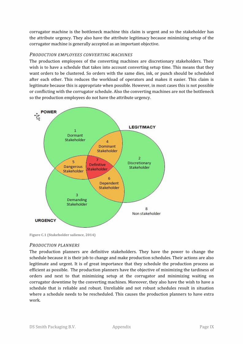
DS Smith Packaging B.V. Appendix Page IX
corrugator machine is the bottleneck machine this claim is urgent and so the stakeholder has
the attribute urgency. They also have the attribute legitimacy because minimizing setup of the
corrugator machine is generally accepted as an important objective.
PRODUCTION EMPLOYEES CONVERTING MACHINES The production employees of the converting machines are discretionary stakeholders. Their
wish is to have a schedule that takes into account converting setup time. This means that they
want orders to be clustered. So orders with the same dies, ink, or punch should be scheduled
after each other. This reduces the workload of operators and makes it easier. This claim is
legitimate because this is appropriate when possible. However, in most cases this is not possible
or conflicting with the corrugator schedule. Also the converting machines are not the bottleneck
so the production employees do not have the attribute urgency.
Figure C.1 (Stakeholder salience, 2014)
PRODUCTION PLANNERS The production planners are definitive stakeholders. They have the power to change the
schedule because it is their job to change and make production schedules. Their actions are also
legitimate and urgent. It is of great importance that they schedule the production process as
efficient as possible. The production planners have the objective of minimizing the tardiness of
orders and next to that minimizing setup at the corrugator and minimizing waiting on
corrugator downtime by the converting machines. Moreover, they also have the wish to have a
schedule that is reliable and robust. Unreliable and not robust schedules result in situation
where a schedule needs to be rescheduled. This causes the production planners to have extra
work.

DS Smith Packaging B.V. Appendix Page X
EXPEDITION PLANNERS The expedition planners are dependent stakeholders. Their actions are both desirable and
urgent. However, they do not have the power to change production schedules. They work with
the schedule that the production planners made. Just like the production planners the
expedition planners wish to have a production schedule that is reliable and robust. When the
schedule changes, there is a probability that an expedition schedule is conflicting.
(PRODUCTION) MANAGEMENT Management is a definitive stakeholder. They have the power, are legitimate, and have urgent
claims. Their objective is a production schedule that results in a production process that
produces maximum output and meets customer demands. This means that they want to
minimize setups and downtimes, because this results in a reduction in throughput. They also
want to minimize the tardiness of orders.
OVERVIEW The stakeholders and their attributes are summarized in Table 1. We can see that there are
three dependent stakeholders, one discretionary stakeholder, and two definitive stakeholders.
Stakeholder Attribute Type stakeholder
Power Legitimacy Urgency
Sales department X X Dependent Production employees corrugator X X Dependent Production employees converting X Discretionary Production planners X X X Definitive Expedition planners X X Dependent (Production) management X X X Definitive Table C.1: Overview stakeholders and their attributes
Out of the stakeholder analysis we found that timeliness of orders, lost production time,
robustness, and ease of working are important objectives and wishes.
Stakeholder Timeliness of orders
Lost production time
Robustness Ease of working
Sales department X Production employees corrugator X X Production employees converting X X Production planners X X X Expedition planners X (Production) Management X X Table C.2: Different objectives for production scheduling

DS Smith Packaging B.V. Appendix Page XI
APPENDIX H: PENTEK OVERVIEW This appendix gives an overview of the Pentek module. Figure H.1 gives a representation of the
fill rate of the Pentek and Figure H.2 gives a representation of the fill rates of the seven different
conveyors and the meters occupied of the conveyors in front of the machines. We also give the
pseude code used to determine the fill rate(s).
Figure H.1 Pentek fill rate
Figure H.2 Overview conveyors

DS Smith Packaging B.V. Appendix Page XII
Pseudo code: MConc,t = 0 MMCont,m = 0 MPo,t = 0 CMOo,t = 0 for (t) do for (s|s=1) do for (o|(FSTo - DTo) ≤ t) do for (c|(slo<WCc and slo≥WCc-1))do for (m|Routeo,s = m and FTJo,m > t) do
,
o,c
1
i
,
|
MCIMP
TPTCImax 1 ;
min TPTCI ; t – STCI
o cici OinCI ci
ci ci
o t
,1
, ,|
, ,
,
,
min ; –
CMO MP * 1 max 0 ;
*
o
o m o mm Route m
o t o t
o t
o m
o
TPTJ t STJ
MPTPTJ
TMO
If MMCont,m < mclm then MMCont,m = MMCont,m + CMOo,t
if MMCont,m > mclm then MConc,t = MConc,t + (MMConm – mclm) MMConm = mclm Endif else MConc,t = MConc,t + CMOo,t
Endif Endfor Endfor Endfor Endfor Endfor For t do For (c|MConc,t > clc and c<7) do MConc+1,t = MConc+1,t + (MConc,t –clc) MConc,t = clc Endfor Endfor FConc,t = MConc,t / clc
,c
t
t
c
c
c
F
MCon
cP
l

DS Smith Packaging B.V. Appendix Page XIII
APPENDIX I: CORRUGATOR AND CONVERTING SCHEDULING OVERVIEW This appendix gives screen shots of the corrugator and converting scheduling modules. In
Figure I.1 the screenshot of the corrugator scheduling module can be found and in Figure I.2 the
converting scheduling module. In the marked areas the performance indicators are shown.
Figure I.1 Corrugator scheduling
Figure I.2 Converting scheduling
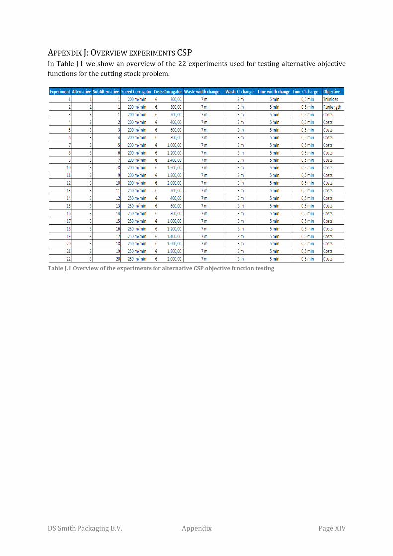
DS Smith Packaging B.V. Appendix Page XIV
APPENDIX J: OVERVIEW EXPERIMENTS CSP In Table J.1 we show an overview of the 22 experiments used for testing alternative objective
functions for the cutting stock problem.
Table J.1 Overview of the experiments for alternative CSP objective function testing

DS Smith Packaging B.V. Appendix Page XV
APPENDIX K: RESULTS ALPHA SETTINGS TESTING This appendix shows the results of the four tests for choosing the best alpha settings.
Alpha 10 15 20 25 30 35 40 45 50 55
average 26.666 22.153 19.744 18.489 17.765 17.305 17.056 16.856 16.749 16.655
max 35.994 28.754 25.215 25.772 21.903 21.798 20.555 20.561 19.837 19.578
min 19.890 16.578 14.435 14.075 14.191 12.848 13.483 13.128 13.207 13.146
St. dv. 2.352 1.997 1.637 1.409 1.170 1.091 1.000 0.981 0.931 0.944 Table K.1 Results of the alpha test for situation 1
Alpha 10 15 20 25 30 35 40 45 50 55
average 12.792 9.931 8.693 8.164 7.903 7.769 7.736 7.724 7.707 7.689
max 17.680 14.430 11.861 11.124 10.708 9.862 9.692 9.395 9.481 9.115
min 8.728 6.744 6.536 6.536 6.536 6.744 6.744 6.744 6.744 6.744
St. dv. 1.514 1.144 0.875 0.724 0.658 0.635 0.617 0.607 0.605 0.601 Table K.2 Results of the alpha test for situation 2
Alpha 10 15 20 25 30 35 40 45 50 55
average 43.828 35.157 30.910 28.524 26.969 26.241 25.685 25.276 25.073 24.980
max 61.035 50.701 47.482 38.381 38.882 36.515 34.411 35.739 36.438 34.638
min 30.566 23.207 21.626 19.624 19.123 16.692 18.192 18.927 17.272 18.470
St. dv. 4.992 3.947 3.407 2.973 2.787 2.528 2.468 2.385 2.369 2.298
Table K.3 Results of the alpha test for situation 3
Alpha 10 15 20 25 30 35 40 45 50 55
average 17.872 13.784 11.221 9.840 9.114 8.745 8.384 8.167 8.004 7.940
max 24.766 20.277 16.090 14.366 13.061 11.888 11.124 11.646 10.734 10.827
min 12.626 9.316 7.596 7.134 6.713 6.651 6.651 6.651 7.003 6.651
St. dv. 1.897 1.611 1.298 1.061 0.911 0.909 0.914 0.897 0.852 0.841 Table K.4 Results of the alpha test for situation 4