Embed Size (px)
DESCRIPTION
This is a lecture note Implicit Euler (part 1) method taught at University of Melbourne. It shows how this method being derived, the stability analysis, error analysis and how to use it with Matlab
Citation preview
ENGR90024 Computational Fluid Dynamics
Lecture O06
The Implicit Euler Method!
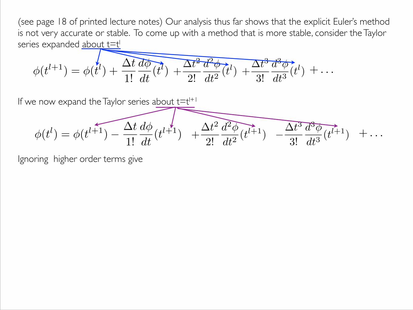
(see page 18 of printed lecture notes) Our analysis thus far shows that the explicit Euler’s method is not very accurate or stable. To come up with a method that is more stable, consider the Taylor series expanded about t=tl
If we now expand the Taylor series about t=tl+1
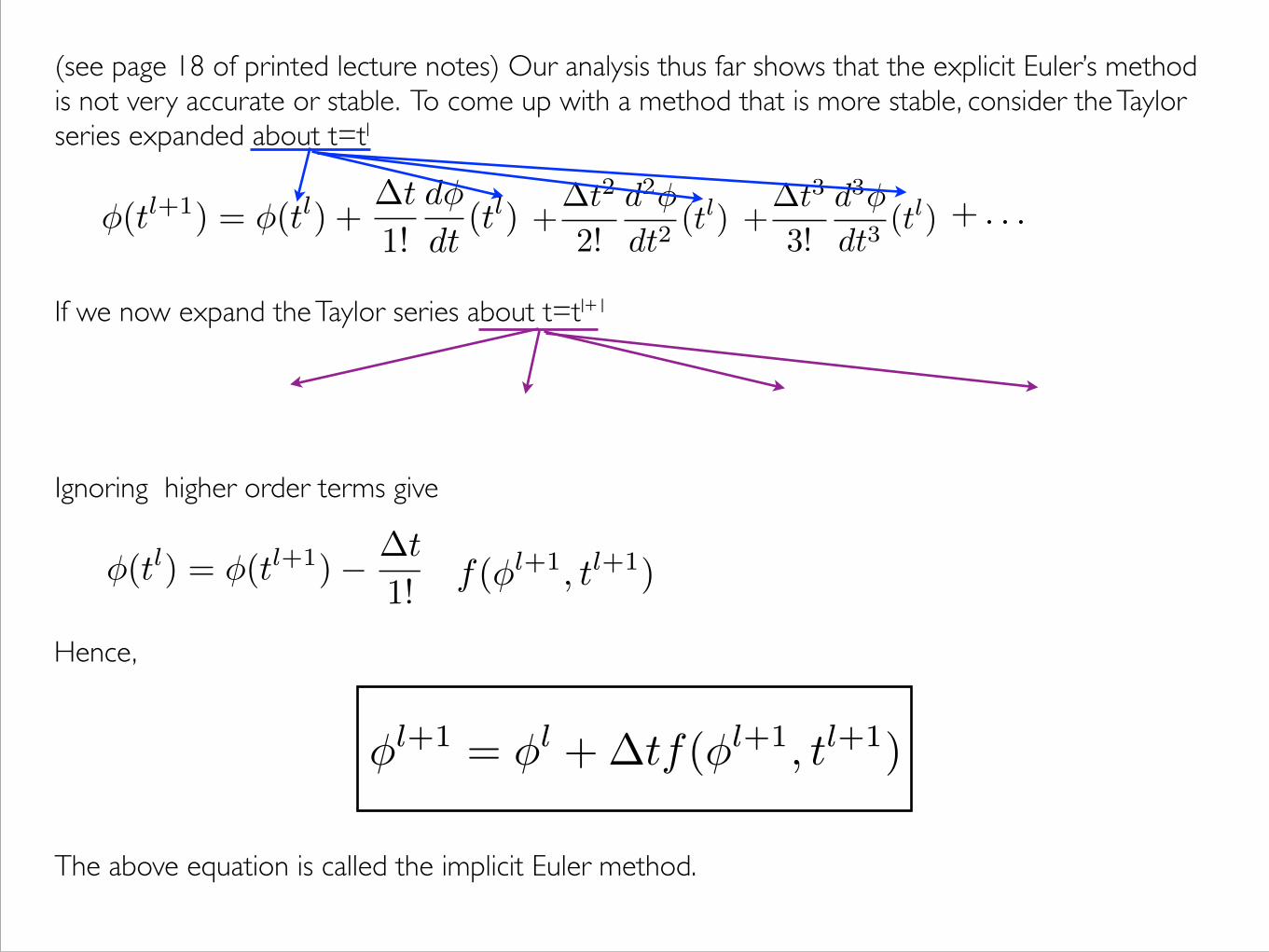
Ignoring higher order terms give
+ . . .
+�t2
2!
d2�
dt2(tl)�(tl+1) = �(tl) +
�t
1!
d�
dt(tl) +
�t3
3!
d3�
dt3(tl) + . . .
�(tl) = �(tl+1)� �t
1!
d�
dt(tl+1) +
�t2
2!
d2�
dt2(tl+1) ��t3
3!
d3�
dt3(tl+1)
(see page 18 of printed lecture notes) Our analysis thus far shows that the explicit Euler’s method is not very accurate or stable. To come up with a method that is more stable, consider the Taylor series expanded about t=tl
If we now expand the Taylor series about t=tl+1
Ignoring higher order terms give
�l+1 = �l +�tf(�l+1, tl+1)
The above equation is called the implicit Euler method.
Hence,
+�t2
2!
d2�
dt2(tl)�(tl+1) = �(tl) +
�t
1!
d�
dt(tl) +
�t3
3!
d3�
dt3(tl) + . . .
�(tl) = �(tl+1)� �t
1!
d�
dt(tl+1)f(�l+1, tl+1)
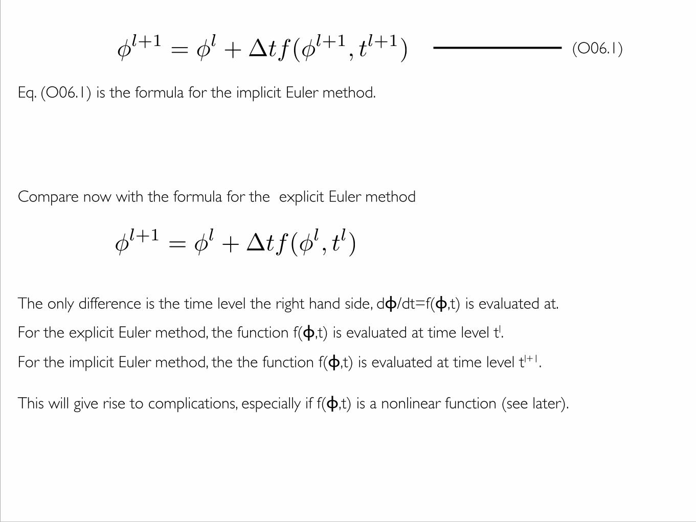
�l+1 = �l +�tf(�l+1, tl+1) (O06.1)
Eq. (O06.1) is the formula for the implicit Euler method.
�l+1 = �l +�tf(�l, tl)
The only difference is the time level the right hand side, dɸ/dt=f(ɸ,t) is evaluated at.
Compare now with the formula for the explicit Euler method
For the explicit Euler method, the function f(ɸ,t) is evaluated at time level tl.
For the implicit Euler method, the the function f(ɸ,t) is evaluated at time level tl+1.
This will give rise to complications, especially if f(ɸ,t) is a nonlinear function (see later).
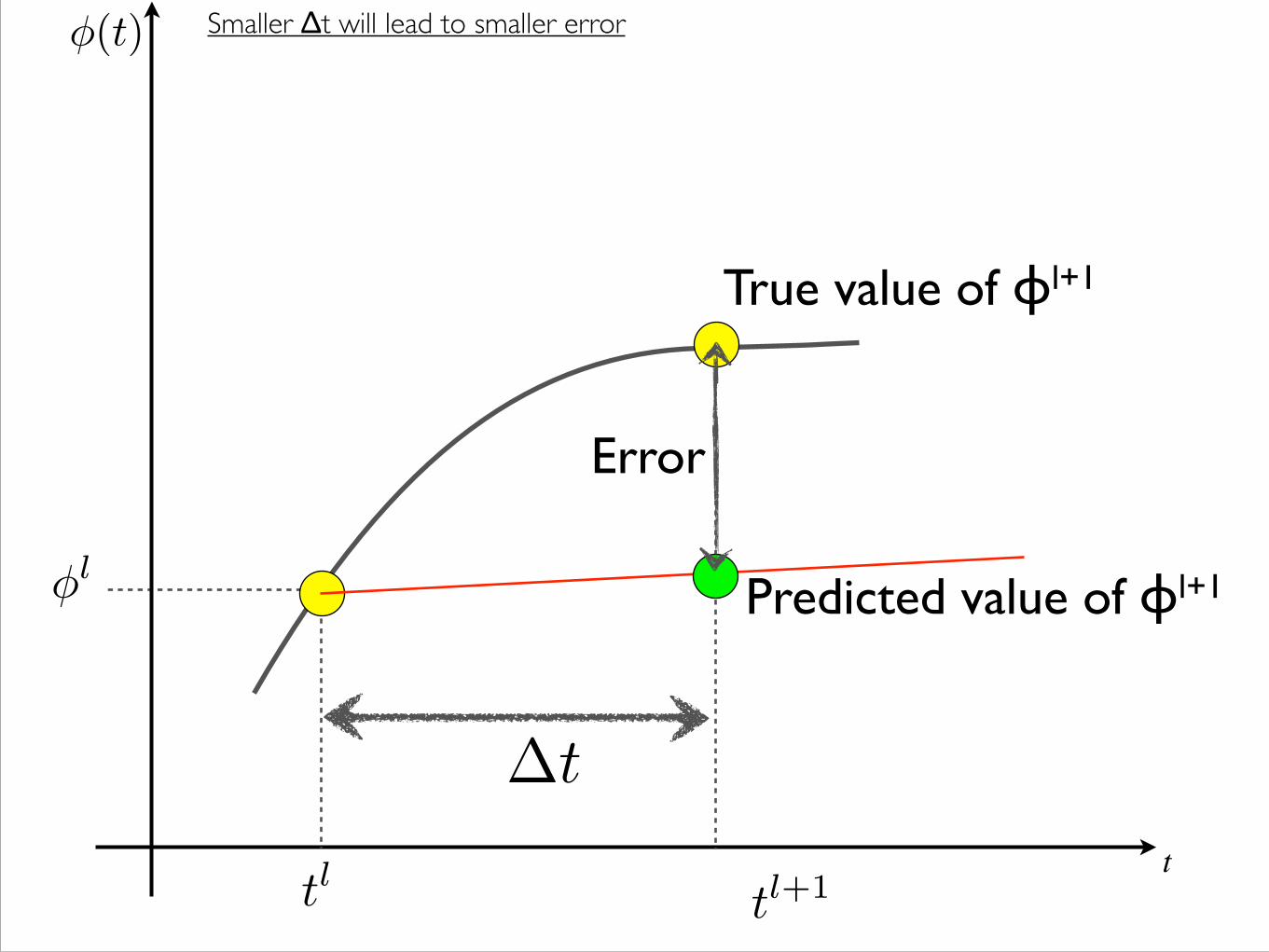
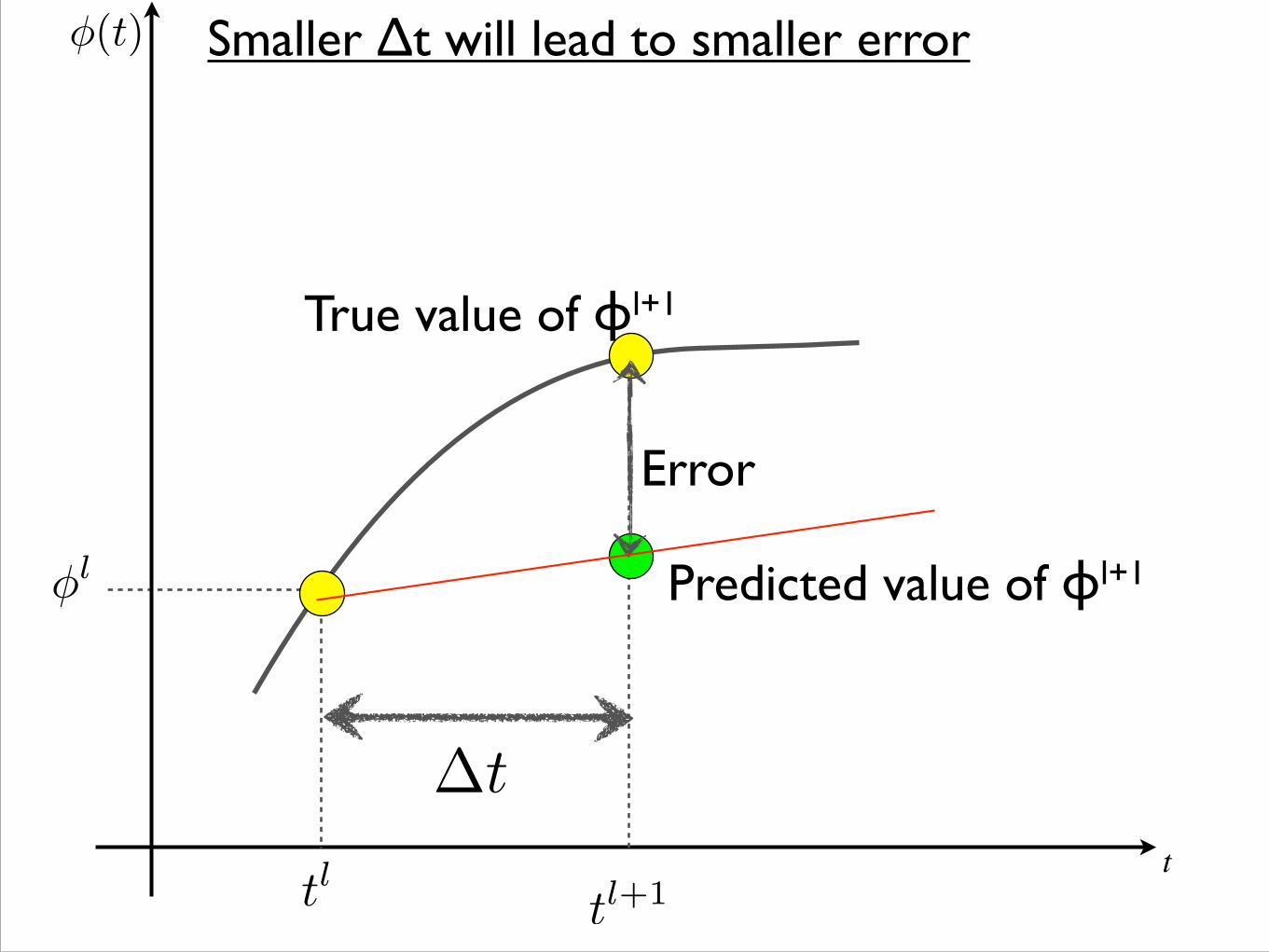
�(t)
tl tl+1
�l
�t
Predicted value of ɸl+1
True value of ɸl+1
Smaller Δt will lead to smaller error
Error
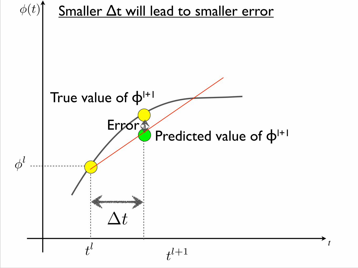
�(t)
�t
tl tl+1
�l Predicted value of ɸl+1
True value of ɸl+1
Smaller Δt will lead to smaller error
Error
�(t)
�t
tl tl+1
�l
Predicted value of ɸl+1
True value of ɸl+1
Smaller Δt will lead to smaller error
Error
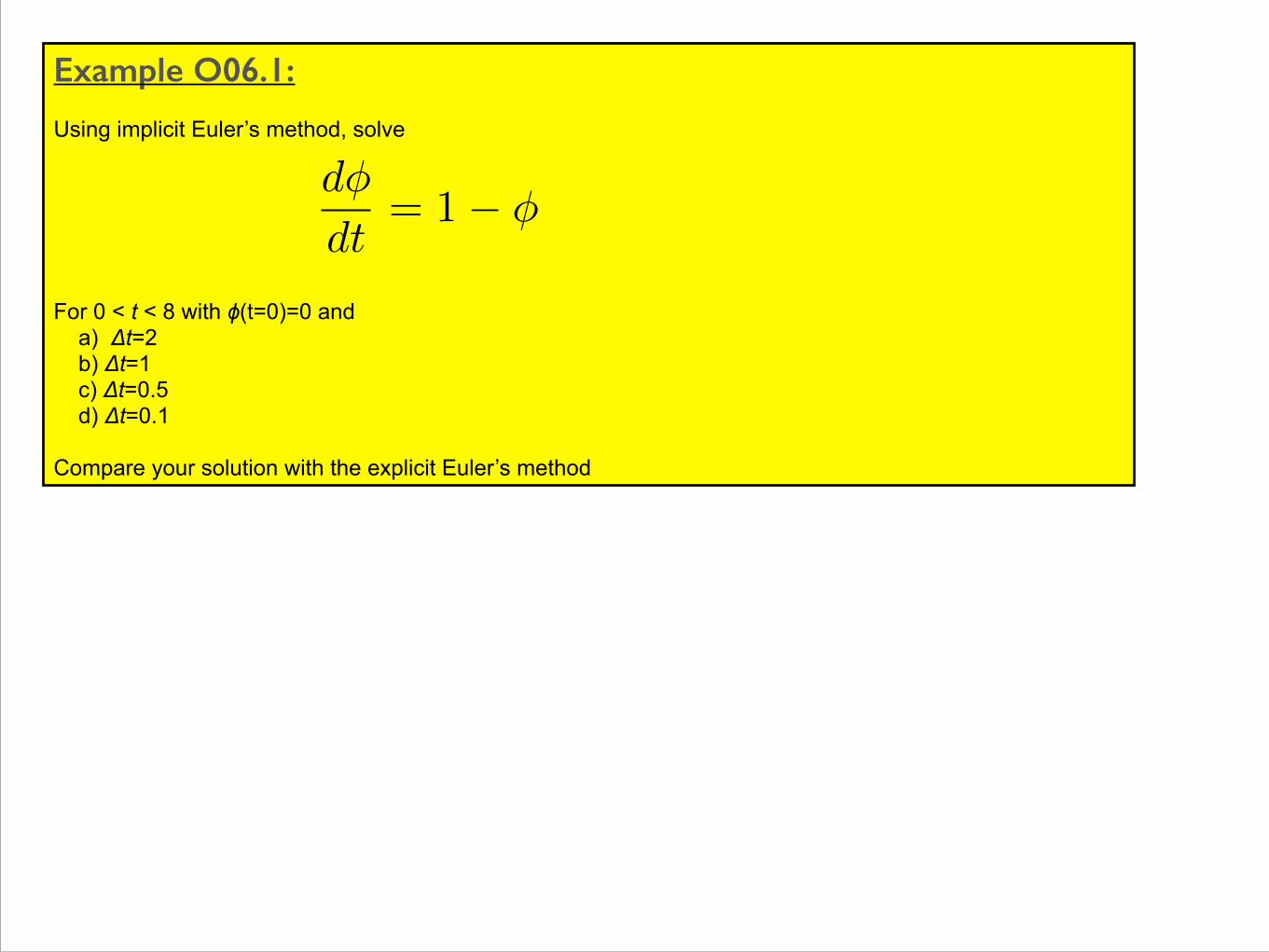
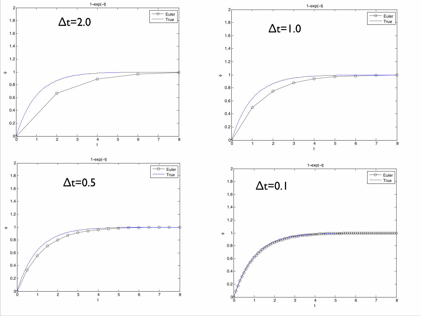
Example O06.1: !Using implicit Euler’s method, solve !!!!!For 0 < t < 8 with ɸ(t=0)=0 and a) Δt=2 b) Δt=1 c) Δt=0.5 d) Δt=0.1 !Compare your solution with the explicit Euler’s method
d�
dt= 1� �
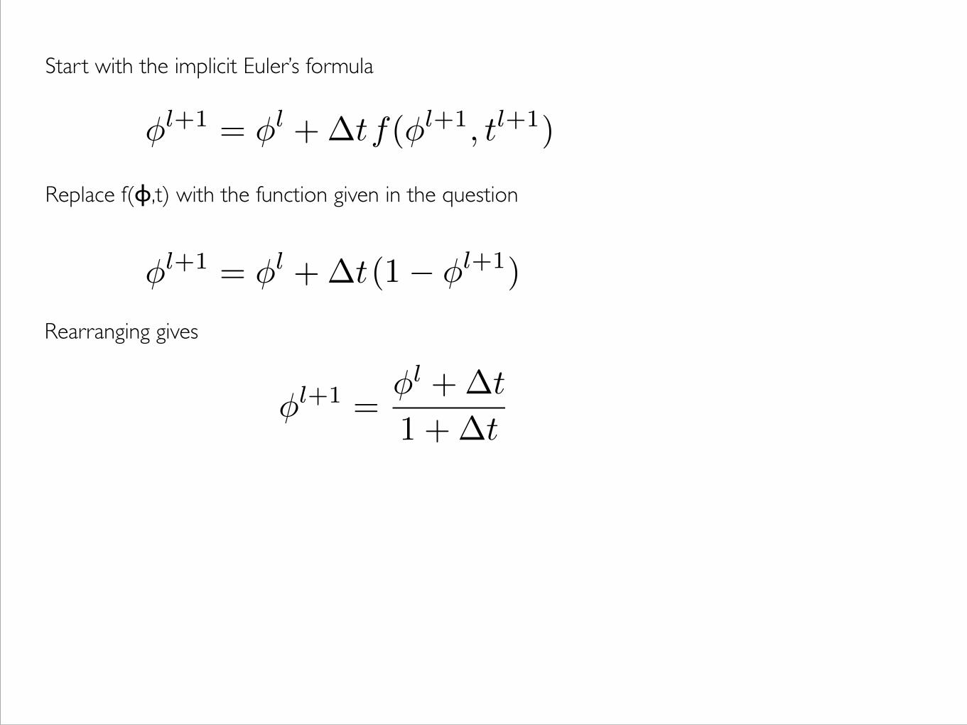
�l+1 = �l +�t
Start with the implicit Euler’s formula
Replace f(ɸ,t) with the function given in the question
(1� �l+1)
�l+1 = �l +�tf(�l+1, tl+1)
Rearranging gives
�l+1 =�l +�t
1 +�t
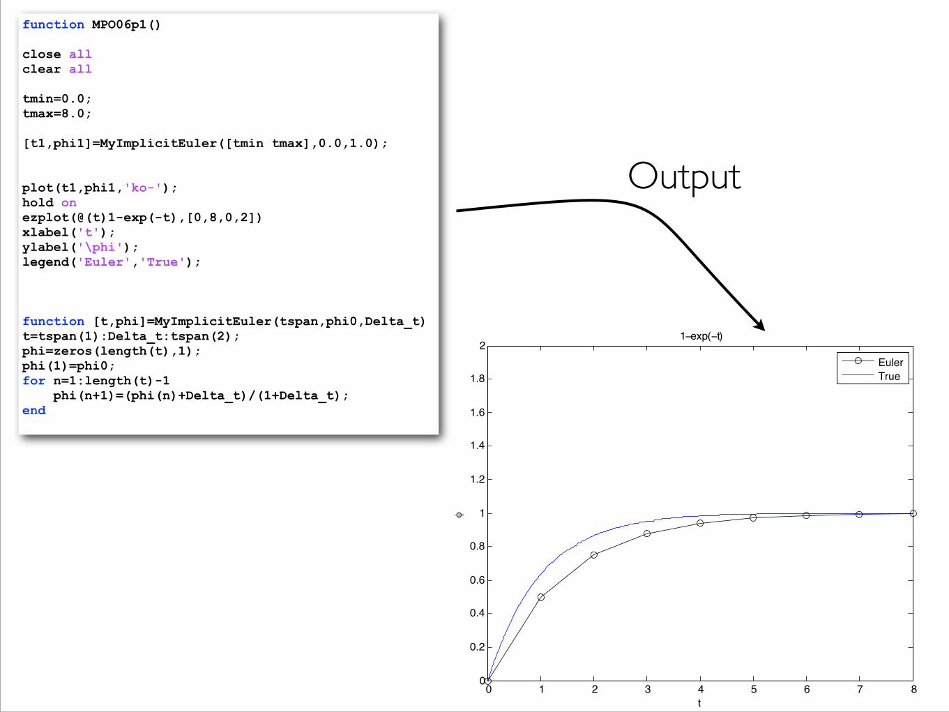
function MPO06p1() close all clear all tmin=0.0; tmax=8.0; [t1,phi1]=MyImplicitEuler([tmin tmax],0.0,1.0); plot(t1,phi1,'ko-'); hold on ezplot(@(t)1-exp(-t),[0,8,0,2]) xlabel('t'); ylabel('\phi'); legend('Euler','True'); function [t,phi]=MyImplicitEuler(tspan,phi0,Delta_t) t=tspan(1):Delta_t:tspan(2); phi=zeros(length(t),1); phi(1)=phi0; for n=1:length(t)-1 phi(n+1)=(phi(n)+Delta_t)/(1+Delta_t); end
0 1 2 3 4 5 6 7 80
0.2
0.4
0.6
0.8
1
1.2
1.4
1.6
1.8
2
t
1−exp(−t)
φ
EulerTrue
Output
0 1 2 3 4 5 6 7 80
0.2
0.4
0.6
0.8
1
1.2
1.4
1.6
1.8
2
t
1−exp(−t)φ
EulerTrue
0 1 2 3 4 5 6 7 80
0.2
0.4
0.6
0.8
1
1.2
1.4
1.6
1.8
2
t
1−exp(−t)
φ
EulerTrue
0 1 2 3 4 5 6 7 80
0.2
0.4
0.6
0.8
1
1.2
1.4
1.6
1.8
2
t
1−exp(−t)
φ
EulerTrue
0 1 2 3 4 5 6 7 80
0.2
0.4
0.6
0.8
1
1.2
1.4
1.6
1.8
2
t
1−exp(−t)
φ
EulerTrue
Δt=2.0 Δt=1.0
Δt=0.5 Δt=0.1
0 1 2 3 4 5 6 7 80
0.2
0.4
0.6
0.8
1
1.2
1.4
1.6
1.8
2
t
1−exp(−t)
φ
EulerTrueΔt=2.0
0 1 2 3 4 5 6 7 80
0.2
0.4
0.6
0.8
1
1.2
1.4
1.6
1.8
2
t
φ
EulerTrueΔt=2.0
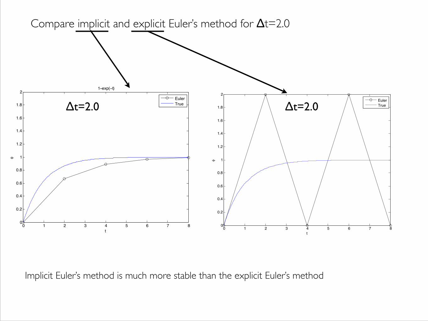
Compare implicit and explicit Euler’s method for Δt=2.0
Implicit Euler’s method is much more stable than the explicit Euler’s method
End of Example O06.1
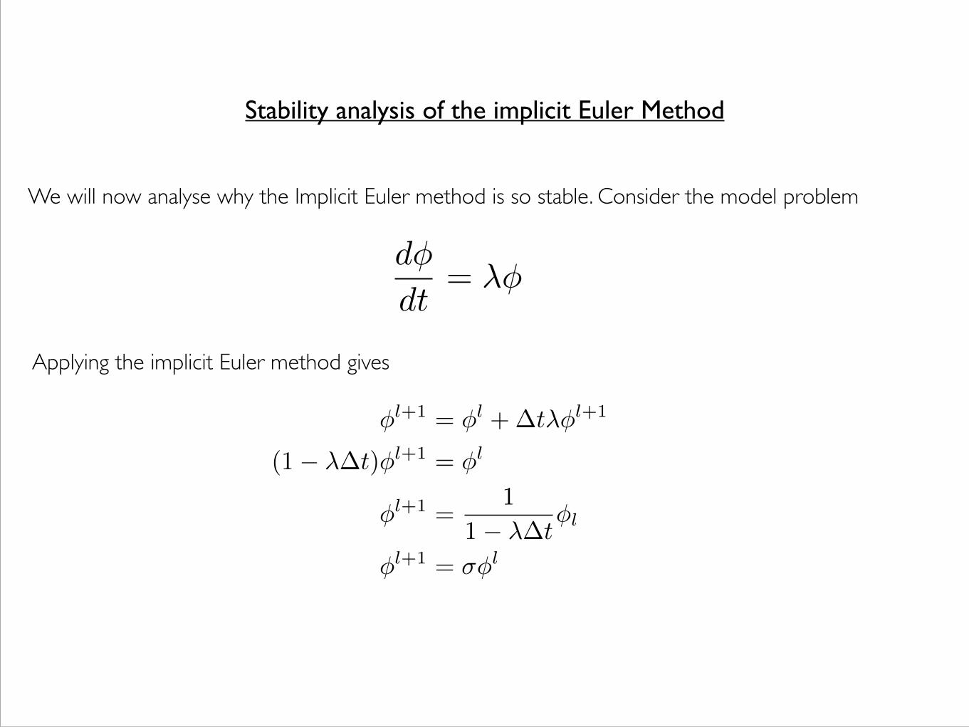
Stability analysis of the implicit Euler Method
We will now analyse why the Implicit Euler method is so stable. Consider the model problem
d�
dt= ��
Applying the implicit Euler method gives
�l+1 = �l +�t��l+1
(1� ��t)�l+1 = �l
�l+1 =1
1� ��t�l
�l+1 = ��l
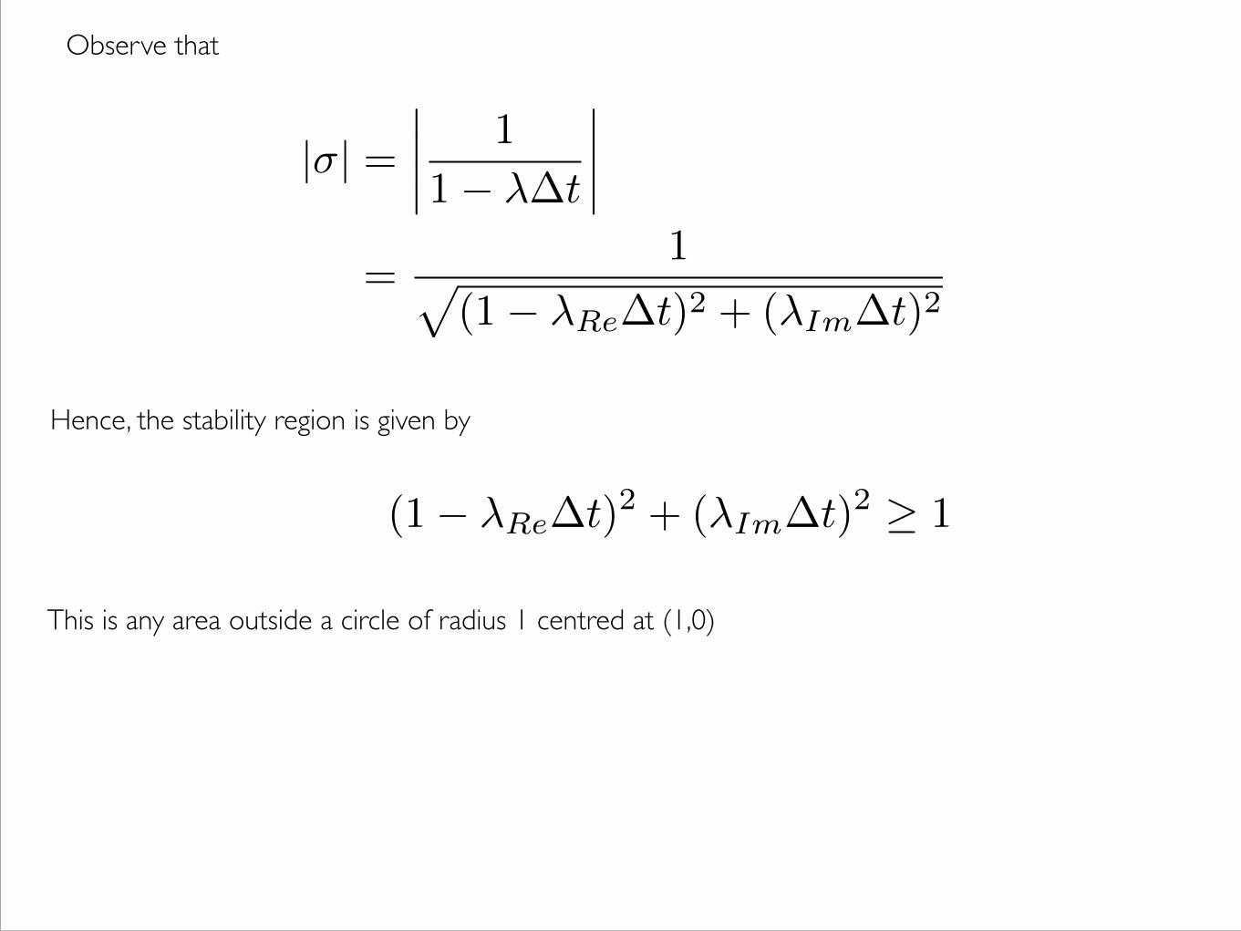
Observe that
|�| =����
1
1� ��t
����
=1p
(1� �Re�t)2 + (�Im�t)2
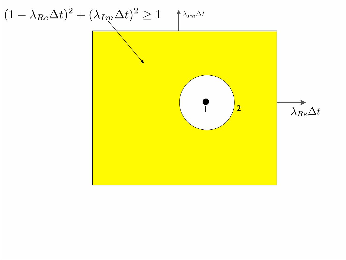
This is any area outside a circle of radius 1 centred at (1,0)
Hence, the stability region is given by
(1� �Re�t)2 + (�Im�t)2 � 1
�Im�t
�Re�t1 2
(1� �Re�t)2 + (�Im�t)2 � 1
�Im�t
�Re�t
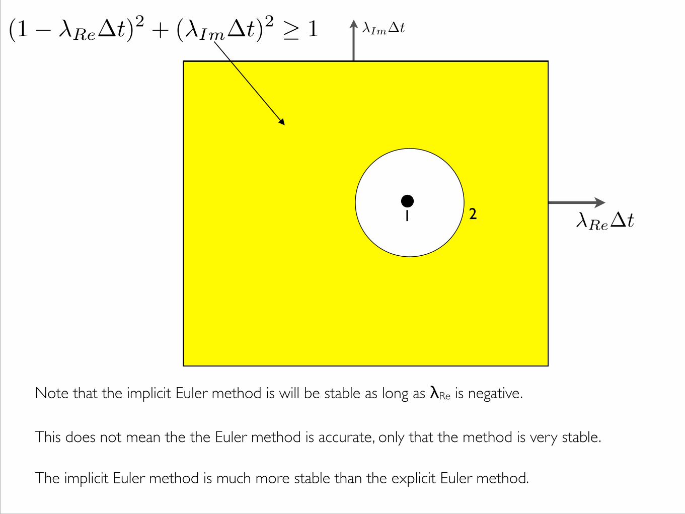
Note that the implicit Euler method is will be stable as long as λRe is negative.
1 2
(1� �Re�t)2 + (�Im�t)2 � 1
This does not mean the the Euler method is accurate, only that the method is very stable.
The implicit Euler method is much more stable than the explicit Euler method.
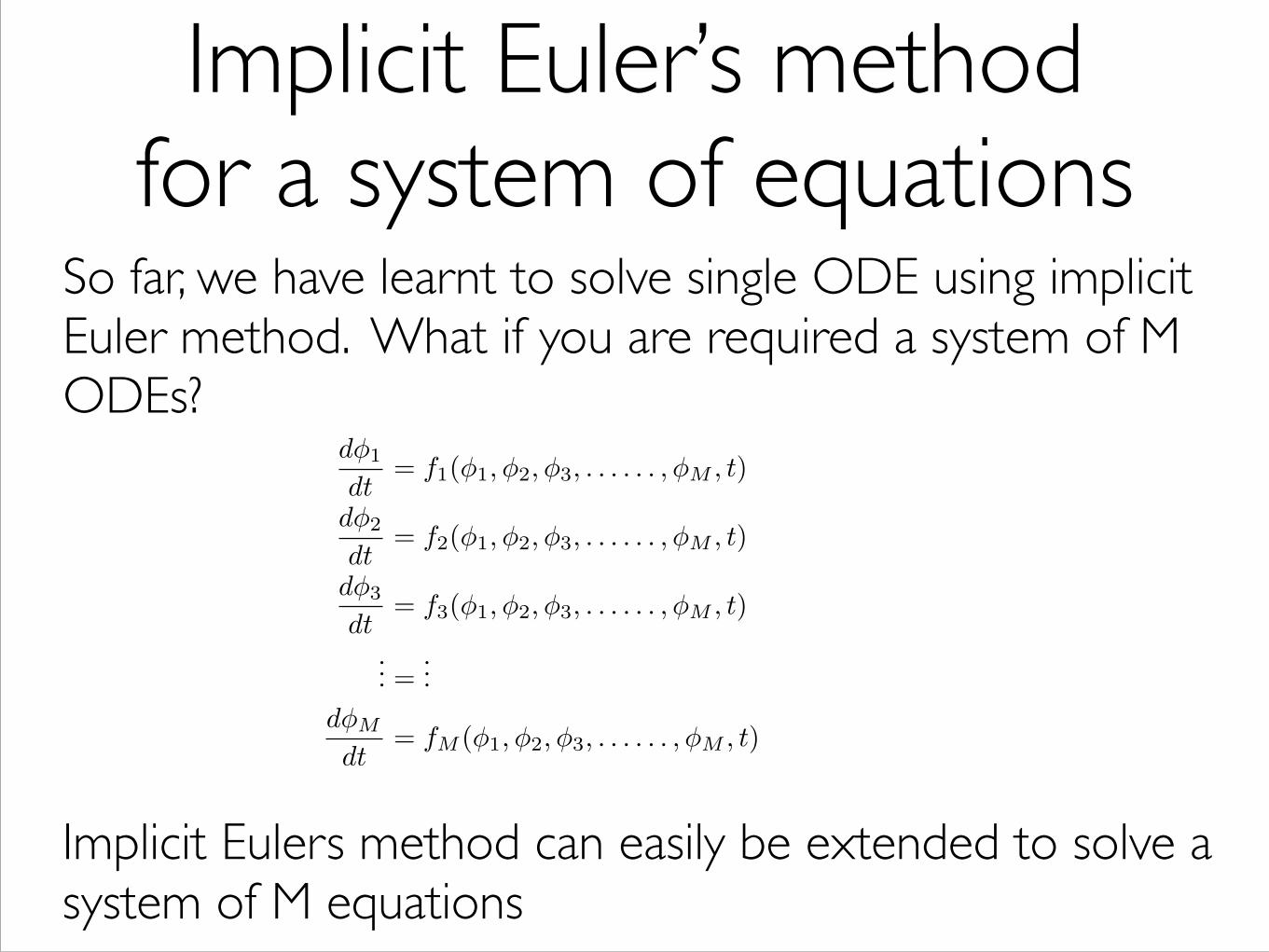
So far, we have learnt to solve single ODE using implicit Euler method. What if you are required a system of M ODEs?
d�1
dt= f1(�1,�2,�3, . . . . . . ,�M , t)
d�2
dt= f2(�1,�2,�3, . . . . . . ,�M , t)
d�3
dt= f3(�1,�2,�3, . . . . . . ,�M , t)
... =...
d�M
dt= fM (�1,�2,�3, . . . . . . ,�M , t)
Implicit Eulers method can easily be extended to solve a system of M equations
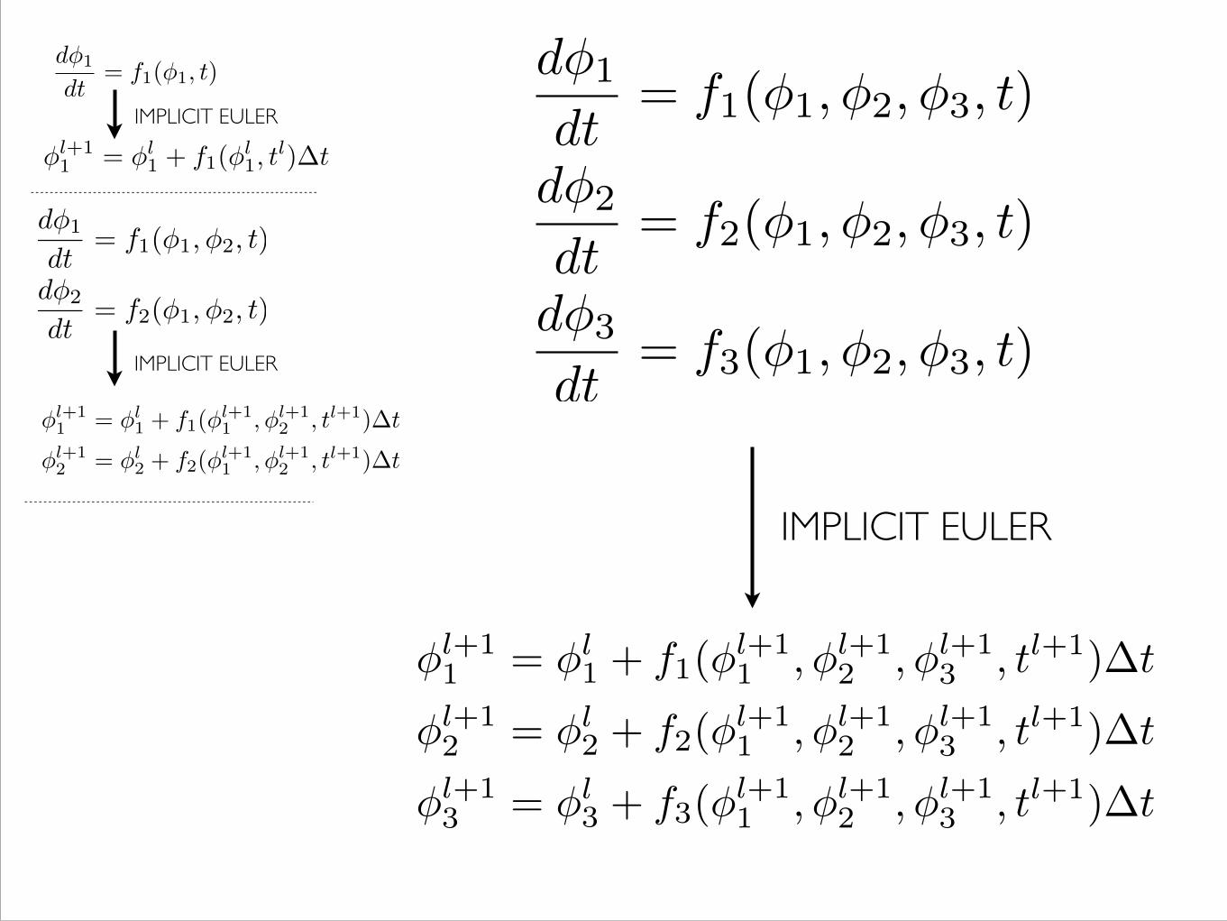
Implicit Euler’s method for a system of equations
d�1
dt= f1(�1,�2, t)
d�2
dt= f2(�1,�2, t)
IMPLICIT EULER
d�1
dt= f1(�1, t)
�l+11 = �l
1 + f1(�l1, t
l)�t
IMPLICIT EULER
IMPLICIT EULER
d�1
dt= f1(�1,�2,�3, t)
d�2
dt= f2(�1,�2,�3, t)
d�3
dt= f3(�1,�2,�3, t)
�l+11 = �l
1 + f1(�l+11 ,�l+1
2 , tl+1)�t
�l+12 = �l
2 + f2(�l+11 ,�l+1
2 , tl+1)�t
�l+11 = �l
1 + f1(�l+11 ,�l+1
2 ,�l+13 , tl+1)�t
�l+12 = �l
2 + f2(�l+11 ,�l+1
2 ,�l+13 , tl+1)�t
�l+13 = �l
3 + f3(�l+11 ,�l+1
2 ,�l+13 , tl+1)�t
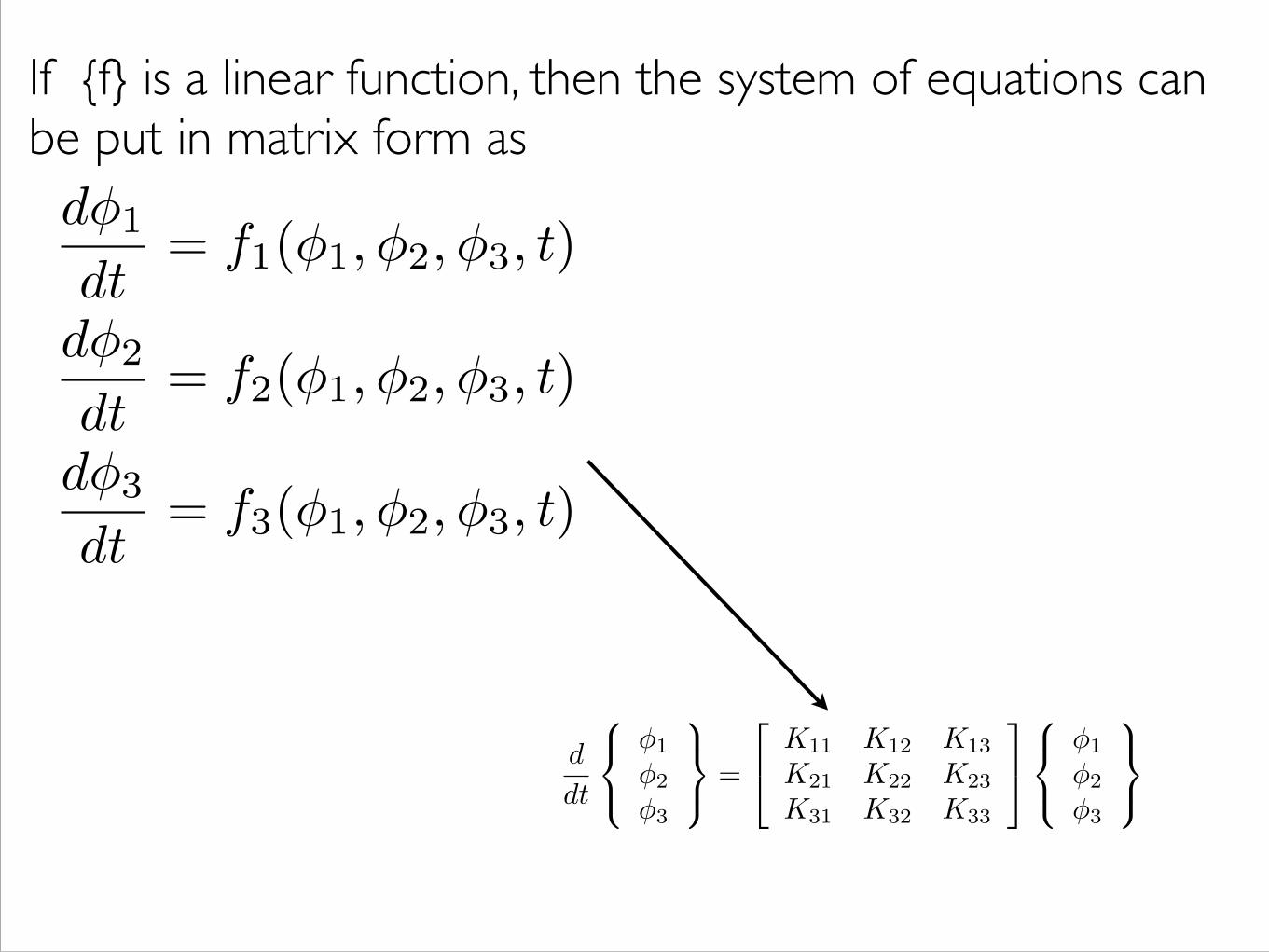
d�1
dt= f1(�1,�2,�3, t)
d�2
dt= f2(�1,�2,�3, t)
d�3
dt= f3(�1,�2,�3, t)
If {f} is a linear function, then the system of equations can be put in matrix form as
d
dt
8<
:
�1
�2
�3
9=
; =
2
4K11 K12 K13
K21 K22 K23
K31 K32 K33
3
5
8<
:
�1
�2
�3
9=
;
d
dt
8<
:
�1
�2
�3
9=
; =
2
4K11 K12 K13
K21 K22 K23
K31 K32 K33
3
5
8<
:
�1
�2
�3
9=
;
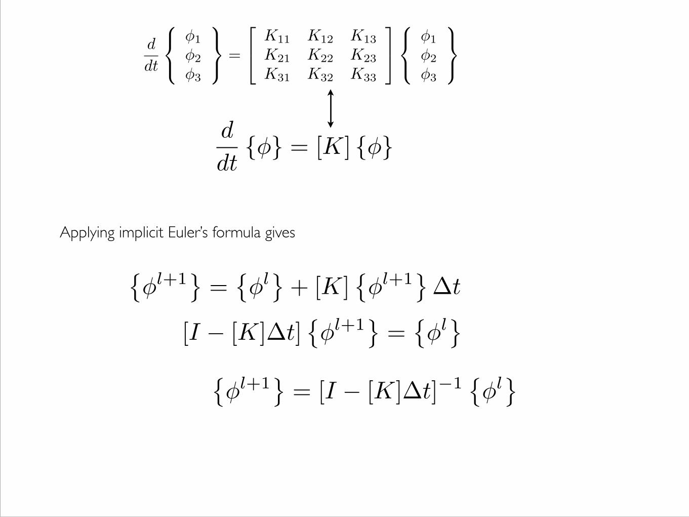
Applying implicit Euler’s formula gives
��l+1
=��l + [K]
��l+1
�t
[I � [K]�t]��l+1
=��l
��l+1
= [I � [K]�t]�1
��l
d
dt{�} = [K] {�}
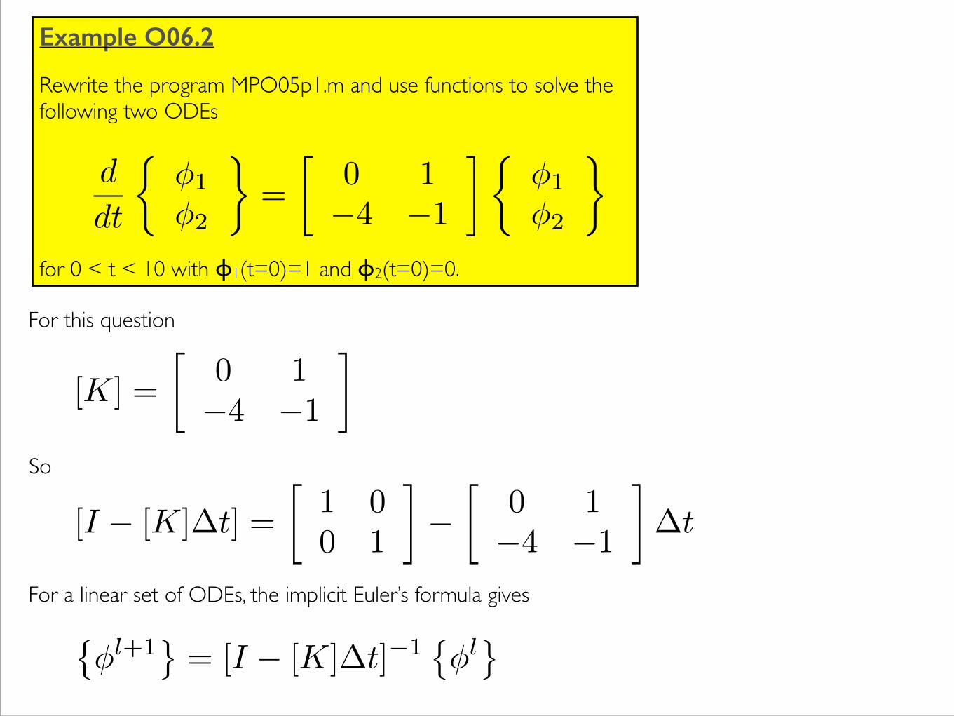
Example O06.2 !Rewrite the program MPO05p1.m and use functions to solve the following two ODEs
!!!!!for 0 < t < 10 with ɸ1(t=0)=1 and ɸ2(t=0)=0.
d
dt
⇢�1
�2
�=
0 1�4 �1
�⇢�1
�2
�
[K] =
0 1�4 �1
�
[I � [K]�t] =
1 00 1
��
0 1�4 �1
��t
For this question
So
��l+1
= [I � [K]�t]�1
��l
For a linear set of ODEs, the implicit Euler’s formula gives
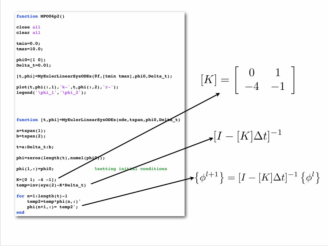
function MPO06p2()! !close all!clear all! !tmin=0.0;!tmax=10.0;! !phi0=[1 0];!Delta_t=0.01;! ![t,phi]=MyEulerLinearSysODEs(@f,[tmin tmax],phi0,Delta_t);! !plot(t,phi(:,1),'k-',t,phi(:,2),'r-');!legend('\phi_1','\phi_2');! ! ! ! !function [t,phi]=MyEulerLinearSysODEs(ode,tspan,phi0,Delta_t)! !a=tspan(1);!b=tspan(2);! !t=a:Delta_t:b;! !phi=zeros(length(t),numel(phi0));! !phi(1,:)=phi0; %setting initial conditions! !K=[0 1; -4 -1];!temp=inv(eye(2)-K*Delta_t)! !for n=1:length(t)-1! temp2=temp*phi(n,:)'! phi(n+1,:)= temp2';!end
[K] =
0 1�4 �1
�
[I � [K]�t]�1
��l+1
= [I � [K]�t]�1
��l
0 1 2 3 4 5 6 7 8 9 10−3
−2
−1
0
1
2
3
φ1
φ2
0 1 2 3 4 5 6 7 8 9 10−3
−2
−1
0
1
2
3
φ1
φ2
0 1 2 3 4 5 6 7 8 9 10−3
−2
−1
0
1
2
3
φ1
φ2
0 1 2 3 4 5 6 7 8 9 10−3
−2
−1
0
1
2
3
φ1
φ2
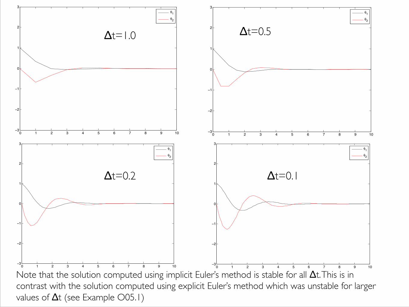
Δt=1.0 Δt=0.5
Δt=0.2
Δt=0.5
Δt=0.1
Note that the solution computed using implicit Euler’s method is stable for all Δt. This is in!contrast with the solution computed using explicit Euler’s method which was unstable for larger!values of Δt (see Example O05.1)
End of Example O06.2

Nonlinear ODEs
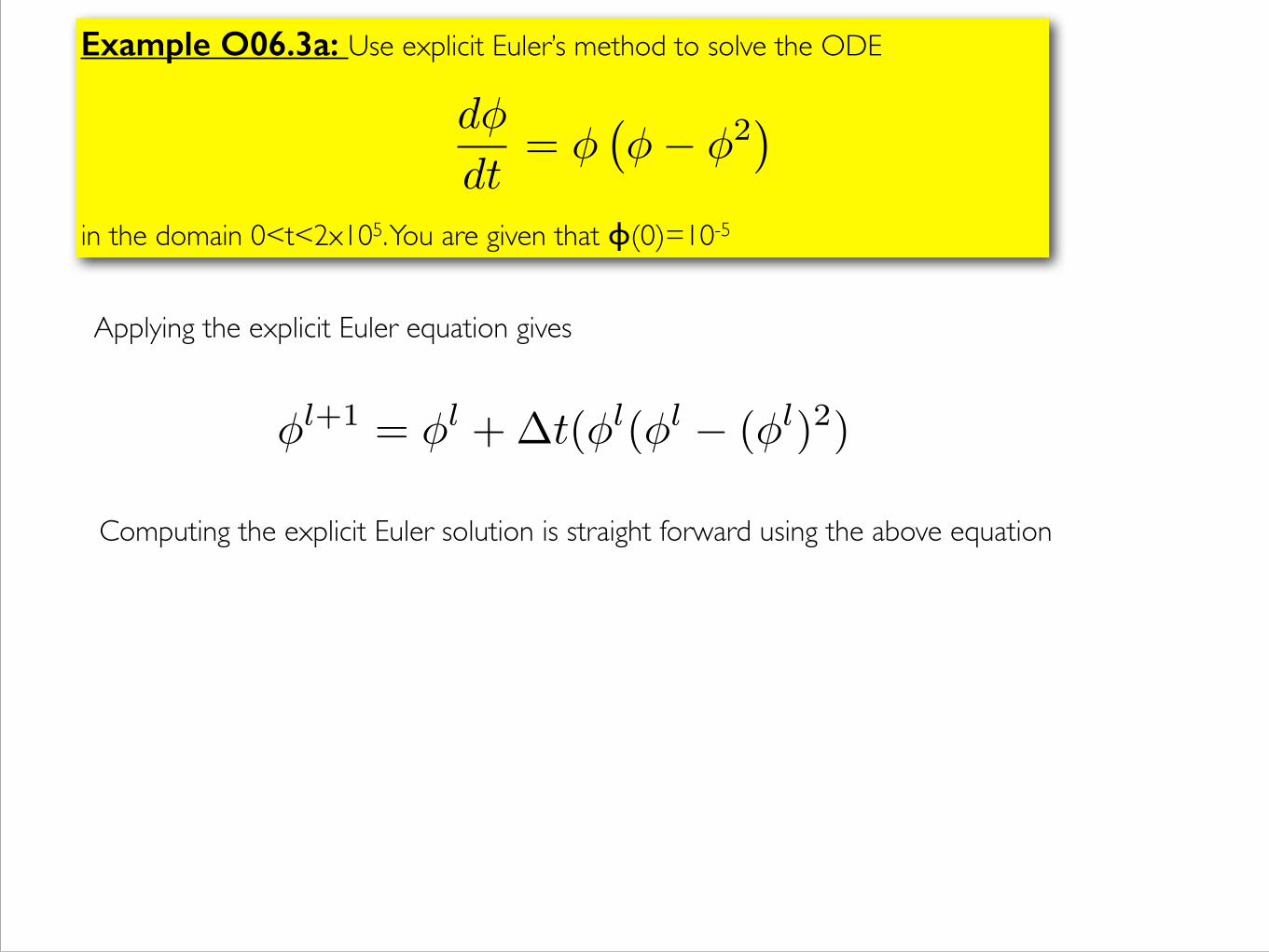
Example O06.3a: Use explicit Euler’s method to solve the ODE!!!!in the domain 0<t<2x10⁵. You are given that ɸ(0)=10-5
d�
dt= �
��� �2
�
�l+1 = �l +�t(�l(�l � (�l)2)
Applying the explicit Euler equation gives
Computing the explicit Euler solution is straight forward using the above equation
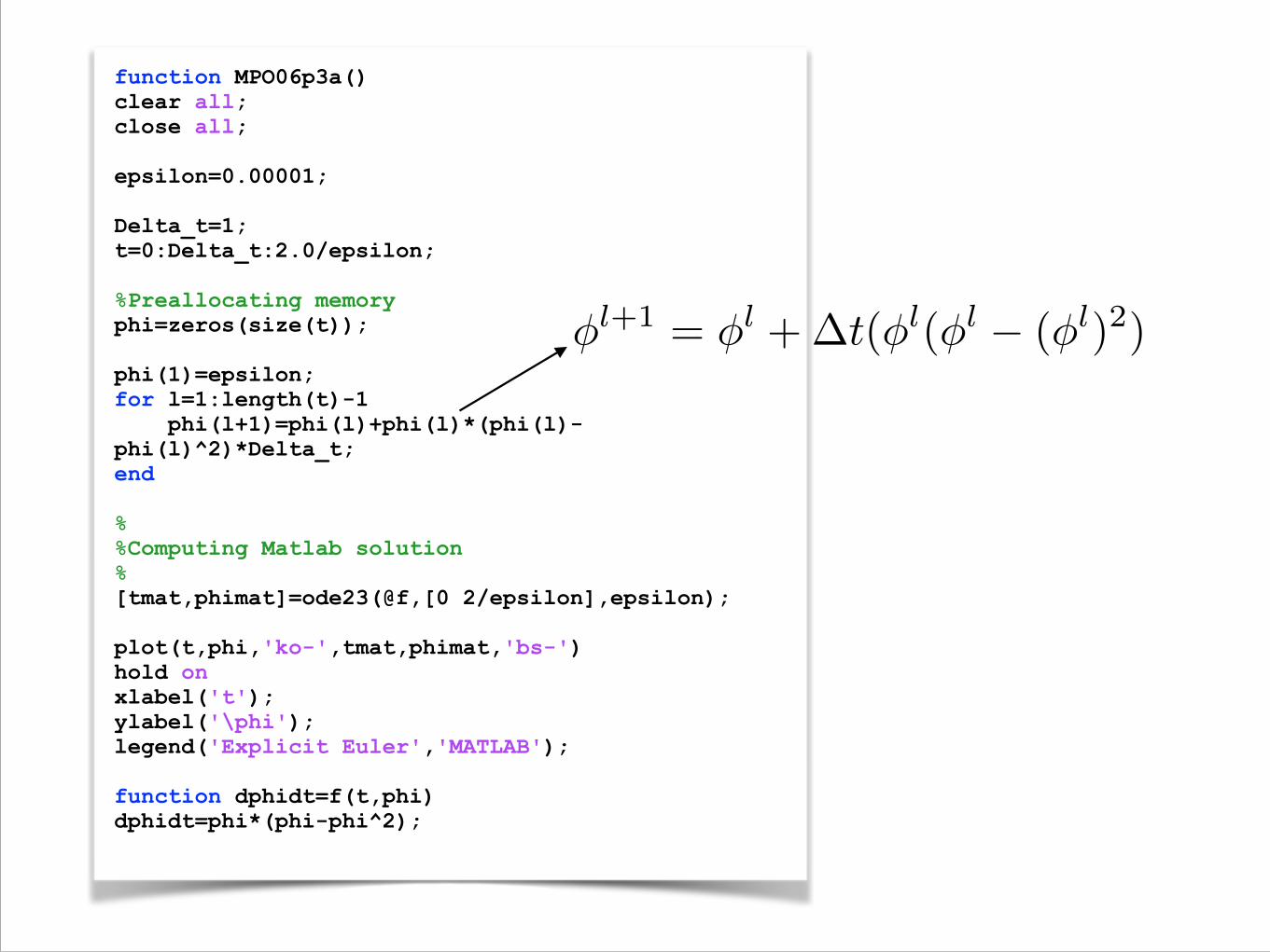
function MPO06p3a() clear all; close all; epsilon=0.00001; Delta_t=1; t=0:Delta_t:2.0/epsilon; %Preallocating memory phi=zeros(size(t)); phi(1)=epsilon; for l=1:length(t)-1 phi(l+1)=phi(l)+phi(l)*(phi(l)-phi(l)^2)*Delta_t; end % %Computing Matlab solution % [tmat,phimat]=ode23(@f,[0 2/epsilon],epsilon); plot(t,phi,'ko-',tmat,phimat,'bs-') hold on xlabel('t'); ylabel('\phi'); legend('Explicit Euler','MATLAB'); function dphidt=f(t,phi) dphidt=phi*(phi-phi^2);
�l+1 = �l +�t(�l(�l � (�l)2)
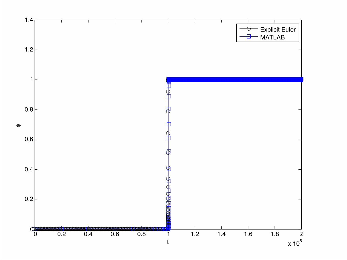
0 0.2 0.4 0.6 0.8 1 1.2 1.4 1.6 1.8 2x 10⁵
0
0.2
0.4
0.6
0.8
1
1.2
1.4
t
φ
Explicit EulerMATLAB
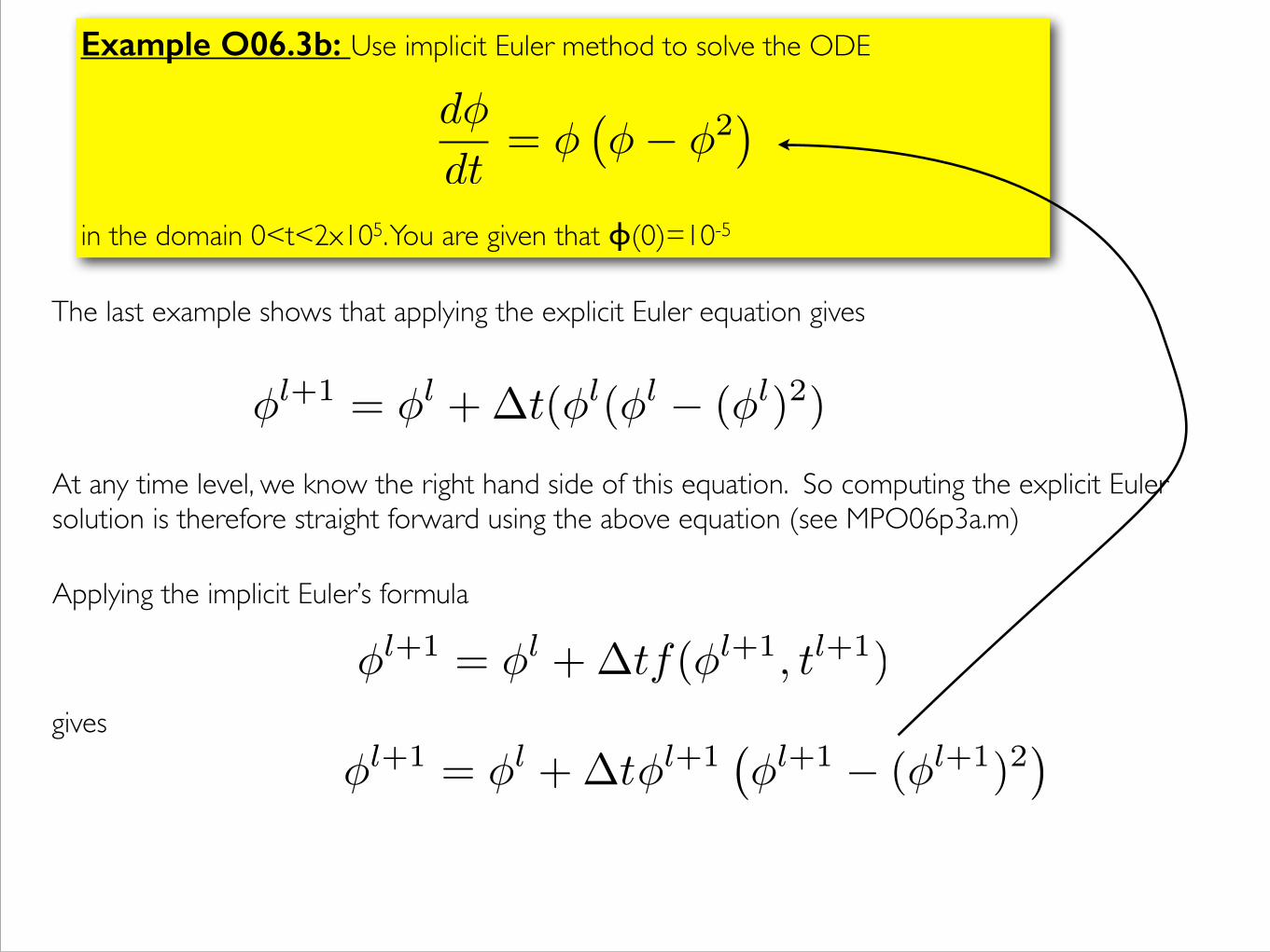
Example O06.3b: Use implicit Euler method to solve the ODE!!!!in the domain 0<t<2x10⁵. You are given that ɸ(0)=10-5
d�
dt= �
��� �2
�
�l+1 = �l +�t(�l(�l � (�l)2)
The last example shows that applying the explicit Euler equation gives
At any time level, we know the right hand side of this equation. So computing the explicit Eulersolution is therefore straight forward using the above equation (see MPO06p3a.m)
Applying the implicit Euler’s formula
�l+1 = �l +�tf(�l+1, tl+1)gives
�l+1 = �l +�t�l+1��l+1 � (�l+1)2
�
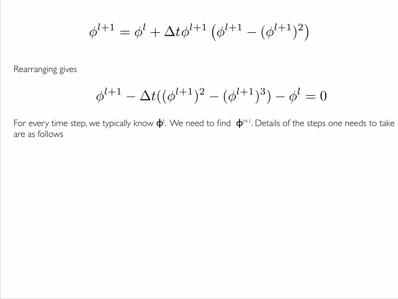
Rearranging gives
For every time step, we typically know ɸl. We need to find ɸl+1. Details of the steps one needs to take are as follows
�l+1 = �l +�t�l+1��l+1 � (�l+1)2
�
�l+1 ��t((�l+1)2 � (�l+1)3)� �l = 0
Solve
to get
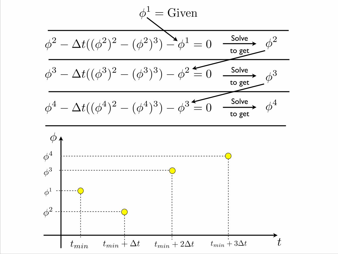
�1 = Given
�2 ��t((�2)2 � (�2)3)� �1 = 0 �2
�3 ��t((�3)2 � (�3)3)� �2 = 0 �3Solve
to get
�4 ��t((�4)2 � (�4)3)� �3 = 0Solve
to get�4
�
ttmin
�1
�2
tmin +�t tmin + 2�t tmin + 3�t
�3
�4
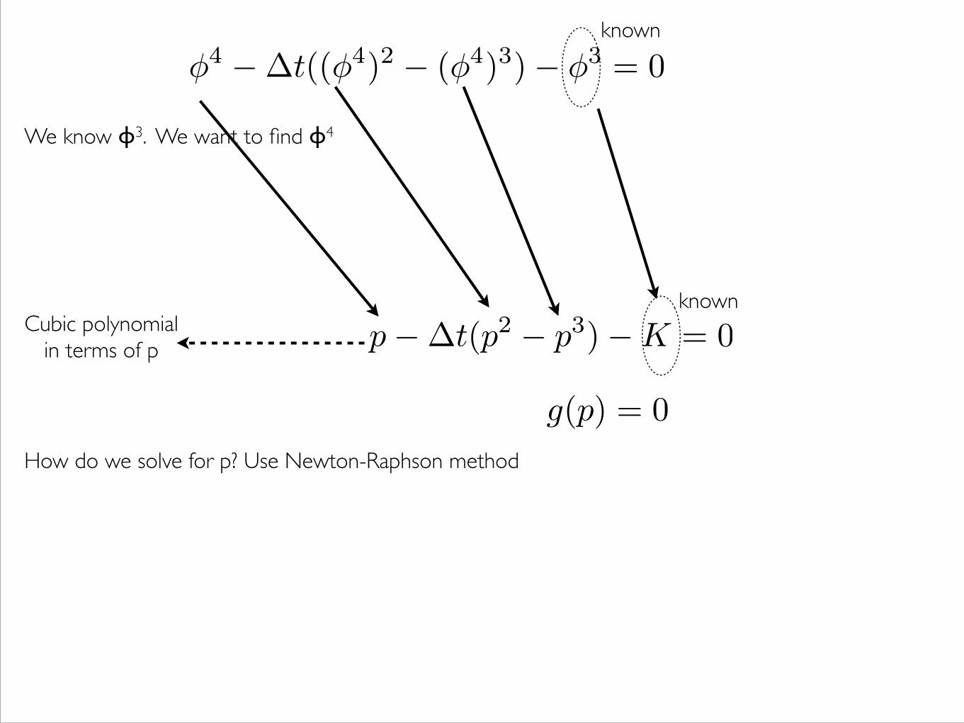
We know ɸ3. We want to find ɸ4
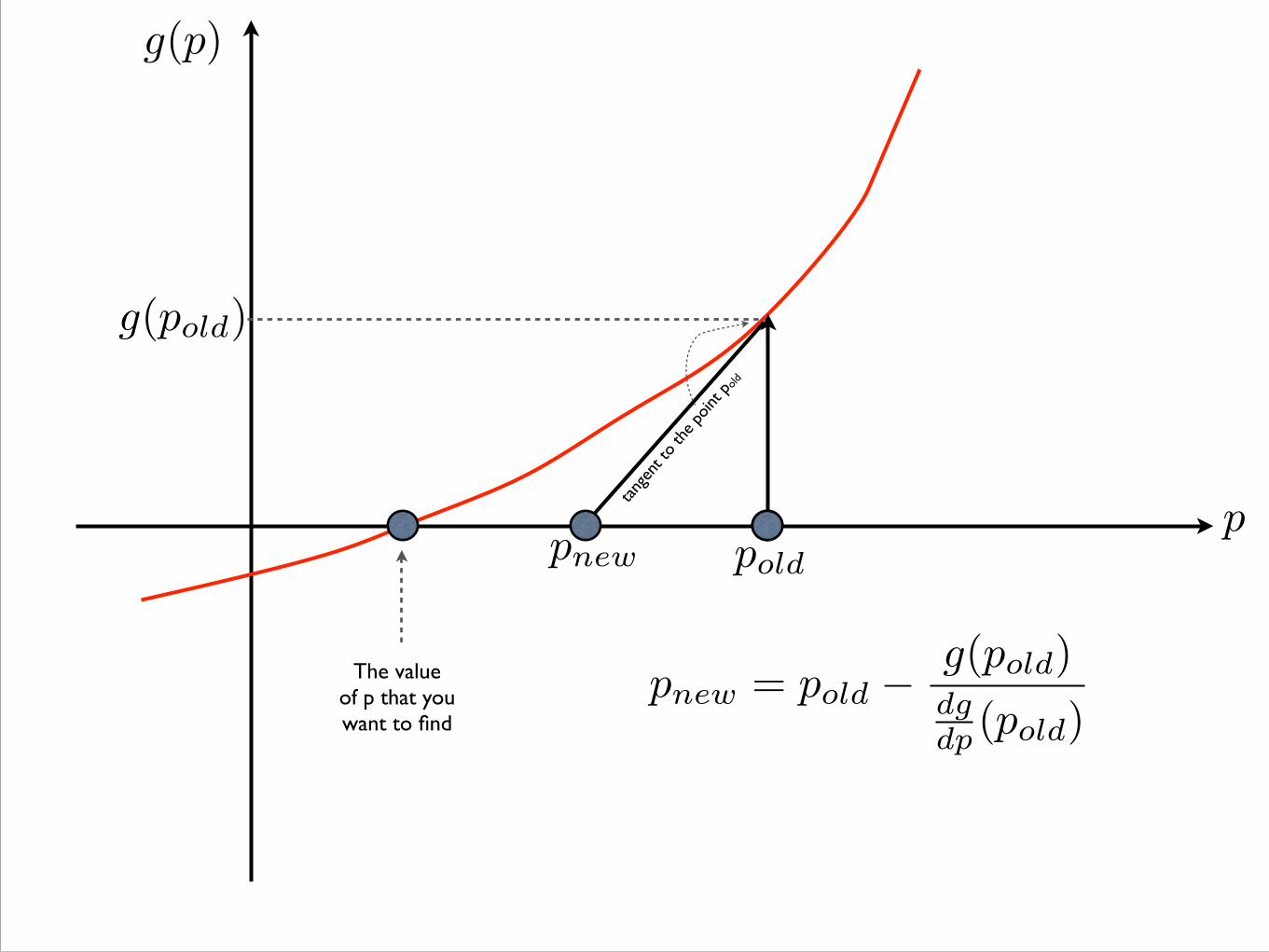
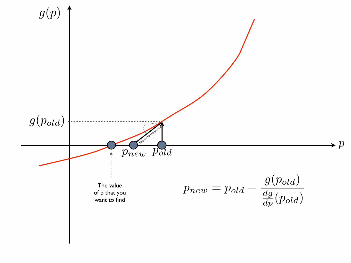
How do we solve for p? Use Newton-Raphson method
g(p) = 0
p��t(p2 � p3)�K = 0
�4 ��t((�4)2 � (�4)3)� �3 = 0known
knownCubic polynomial!
in terms of p
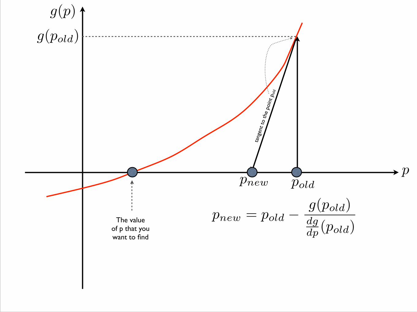
p
The value!of p that you!want to find
pnew pold
tang
ent
to t
he p
oint
pol
d
g(p)
g(pold
)
pnew
= pold
� g(pold
)dg
dp
(pold
)
p
The value!of p that you!want to find
pold
tange
nt to
the p
oint p
old
pnew
g(p)
g(pold
)
pnew
= pold
� g(pold
)dg
dp
(pold
)
p
The value!of p that you!want to find
pold
tangen
t to th
e point
pold
pnew
g(p)
g(pold
)
pnew
= pold
� g(pold
)dg
dp
(pold
)
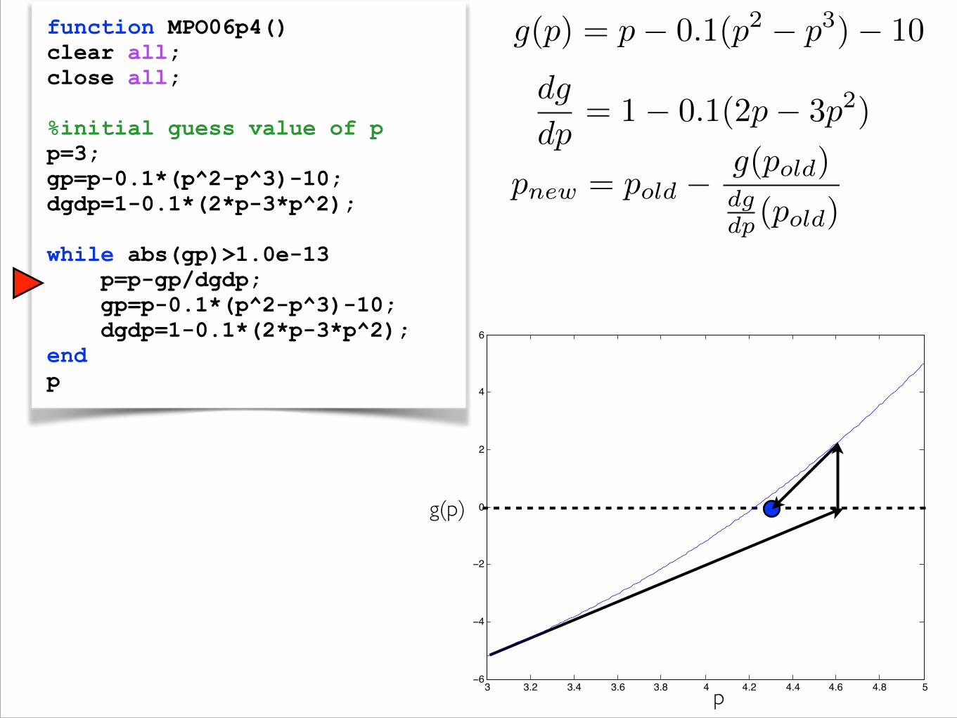
function MPO06p4() clear all; close all; %initial guess value of p p=3; gp=p-0.1*(p^2-p^3)-10; dgdp=1-0.1*(2*p-3*p^2); while abs(gp)>1.0e-13 p=p-gp/dgdp; gp=p-0.1*(p^2-p^3)-10; dgdp=1-0.1*(2*p-3*p^2); end p
pnew
= pold
� g(pold
)dg
dp
(pold
)
g(p) = p� 0.1(p2 � p3)� 10
dg
dp= 1� 0.1(2p� 3p2)
3 3.2 3.4 3.6 3.8 4 4.2 4.4 4.6 4.8 5−6
−4
−2
0
2
4
6
g(p)
p