Numerical methods for ordinary differential equations

Ulrik Skre Fjordholm

May 1, 2018

Chapter 1

Introduction

Consider the ordinary differential equation (ODE)

Px.t/ D f .x.t/; t/; x.0/ D x0 (1.1)

where x0 2 Rd and f W Rd �R! Rd . Under certain conditions on f there exists a unique solutionof (1.1), and for certain types of functions f (such as when (1.1) is separable) there are techniquesavailable for computing this solution. However, for most “real-world” examples of f , we have noidea how the solution actually looks like. We are left with no choice but to approximate the solutionx.t/.

Assume that we would like to compute the solution of (1.1) over a time interval t 2 Œ0; T � forsome T > 01. The most common approach to finding an approximation of the solution of (1.1) startsby partitioning the time interval into a set of points t0; t1; : : : ; tN , where tn D nh is a time step andh D T

Nis the step size2. A numerical method then computes an approximation of the actual solution

value x.tn/ at time t D tn. We will denote this approximation by yn. The basis of most numericalmethods is the following simple computation: Integrate (1.1) over the time interval Œtn; tnC1� to get

x.tnC1/ D x.tn/C

Z tnC1

tn

f .x.s/; s/ ds: (1.2)

Although we could replace x.tn/ and x.tnC1/ by their approximations yn and ynC1, we cannot usethe formula (1.2) directly because the integrand depends on the exact solution x.s/. What we cando, however, is to approximate the integral in (1.2) by some quadrature rule, and then approximatex at the quadrature points. More specifically, we consider a quadrature ruleZ tnC1

tn

g.s/ ds � .tnC1 � tn/

KXkD1

bkg.s.k//

where g is any function, b1; : : : ; bk 2 R are quadrature weights and s.1/; : : : ; s.K/ 2 Œtn; tnC1� arethe quadrature points. Two basic requirements of this approximations is that if g is nonnegativethen the quadrature approximation is also nonnegative, and that the rule correctly integrates constantfunctions. It is straightforward to see that these requirements translate to

b1; : : : ; bk > 0 and b1 C � � � C bK D 1:

1In this note we will only consider a time interval t 2 Œ0; T � for some positive endtime T > 0, but is it fully possible towork with negative times or even the whole real line t 2 R.

2The more sophisticated adaptive time stepping methods use a step size hwhich can change from one time step to another.We will not consider such methods in this note.

1

Some popular methods include the midpoint rule (K D 1, b1 D 1, s.1/ D tnCtnC1

2), the trapezoidal

rule (K D 2, b1 D b2 D12

, s.1/ D tn, s.2/ D tnC1) and Simpson’s rule (K D 3, b1 D b3 D16

,b2 D

46

, s.1/ D tn, s.2/ D tnCtnC1

2, s.3/ D tnC1). As you might recall, these three methods have

an error of O.h3/, O.h3/ and O.h4/, respectively, where h D tnC1 � tn denotes the length of theinterval3.

Applying the quadrature rule to (1.2) yields

ynC1 D yn C h

KXkD1

bkf�y.k/n ; s.k/n

�(1.3)

where s.k/n 2 Œtn; tnC1� are the quadrature points and y.k/n � x�s.k/n

�. The initial approximation y0

is simply set to the initial data prescribed in (1.1), y0 D x0.If the quadrature points y.k/n ; s

.k/n are either yn; tn or ynC1; tnC1 (or some combination of these)

then we can solve (1.3) for ynC1 and get a viable numerical method for (1.1). Two such methods,the explicit and implicit Euler methods, are the topic of Chapter 2. However, if we want to constructmore accurate numerical methods then we have to include quadrature points at times s.k/n which liestrictly between tn and tnC1, and consequently we need some way of computing the intermediatevalues y.k/n � x

�s.k/n

�. A systematic way of computing these points is the so-called Runge–Kutta

methods. These are methods which converge to the exact solution much faster than the Euler meth-ods, and will be the topic of Chapter 4.

Some natural questions arise when deriving numerical methods for (1.1): How large is the ap-proximation error for a fixed step size h > 0? Do the computed solutions converge to x.t/ as h! 0?How fast do they converge, and can we increase the speed of convergence? Is the method stable?The purpose of these notes is to answer all of these questions for some of the most commonly usednumerical methods for ODEs.

Basic assumptionsIn this note we will assume f is continuously differentiable, is bounded and has bounded firstderivatives—that is, we assume that f 2 C 1.R � Rd ;Rd / and that there are constants M > 0

and K > 0 such thatsupx2Rd

t2R

jf .x; t/j 6M; (1.4a)

sup.x;t/Rd�R

Dxf .x; t/ 6 K; (1.4b)

sup.x;t/Rd�R

ˇ̌̌̌@f

@t.x; t/

ˇ̌̌̌6 K: (1.4c)

(Here, Dxf denotes the Jacobian matrix of f ,�Dxf .x; t/

�i;jD

@f i

@xj .x; t/, and k � k denotes thematrix norm.) In particular, f is Lipschitz in x with Lipschitz constant K, so these assumptionsguarantee that Picard iterations converge, and we can conclude that there exists a solution for alltimes t 2 R. Uniqueness of the solution follows from Lipschitz boundedness of f together withGronwall’s lemma.

3Here we use the “Big O notation”. If eh is some quantity depending on a parameter h > 0 (such as the error in anumerical approximation), then eh D O.h

p/ means that there exists some constant C > 0 such that for small values of h,we can bound the error as jehj 6 Chp .

2

The assumptions in (1.4) can be replaced by local bounds, although one then needs to be morecareful in some of the computations in this note. In particular, the solution might not exist for alltimes. Without going into detail we state here that all the results in this note are true (with minormodifications) assuming only local versions of the bounds (1.4).

3

Chapter 2

Euler’s methods

The absolutely simplest quadrature rule that we can use in (1.3) is the one-point method K D 1,b1 D 1, s.1/n D tn. This yields the forward Euler or explicit Euler method

ynC1 D yn C hf�yn; tn

�: (2.1)

As its name implies, this method is explicit, meaning that the approximation ynC1 at the next timestep is given by a formula depending only on the approximation yn at the current time step. Explicitmethods are easy to use on a computer because we can type the formula more or less directly in thesource code. Another popular one-point quadrature is K D 1, b1 D 1, s.1/n D tnC1, which gives thebackward Euler or implicit Euler method

ynC1 D yn C hf�ynC1; tnC1

�: (2.2)

This method is implicit in the sense that one has to solve an algebraic relation in order to find ynC1as a function of only yn. Both of the Euler methods can be seen as first-order Taylor expansions ofx.t/ around t D tn and t D tnC1, respectively.

2.1 Example. Consider the ODE (1.1) with n D 1 and f .x/ D ax for some a 2 R. The forwardEuler method is

ynC1 D yn C hf .yn/ D yn�1C ah

�:

The implicit Euler method is

ynC1 D yn C hf .ynC1/ D yn C ahynC1;

and solving for ynC1 yields the explicit expression

ynC1 Dyn

1 � ah:

In both cases the method can be written as the difference equation ynC1 D byn, whose solution isyn D bnx0. Thus, the explicit Euler method can be written as yn D .1C ah/nx0 and the implicitEuler method as yn D .1 � ah/�nx0. Using the fact that h D T

N, it is a straightforward exercise

in calculus to show that for either scheme, the endtime solution yN converges to the exact valuex.T / D eaT x0 as N !1.

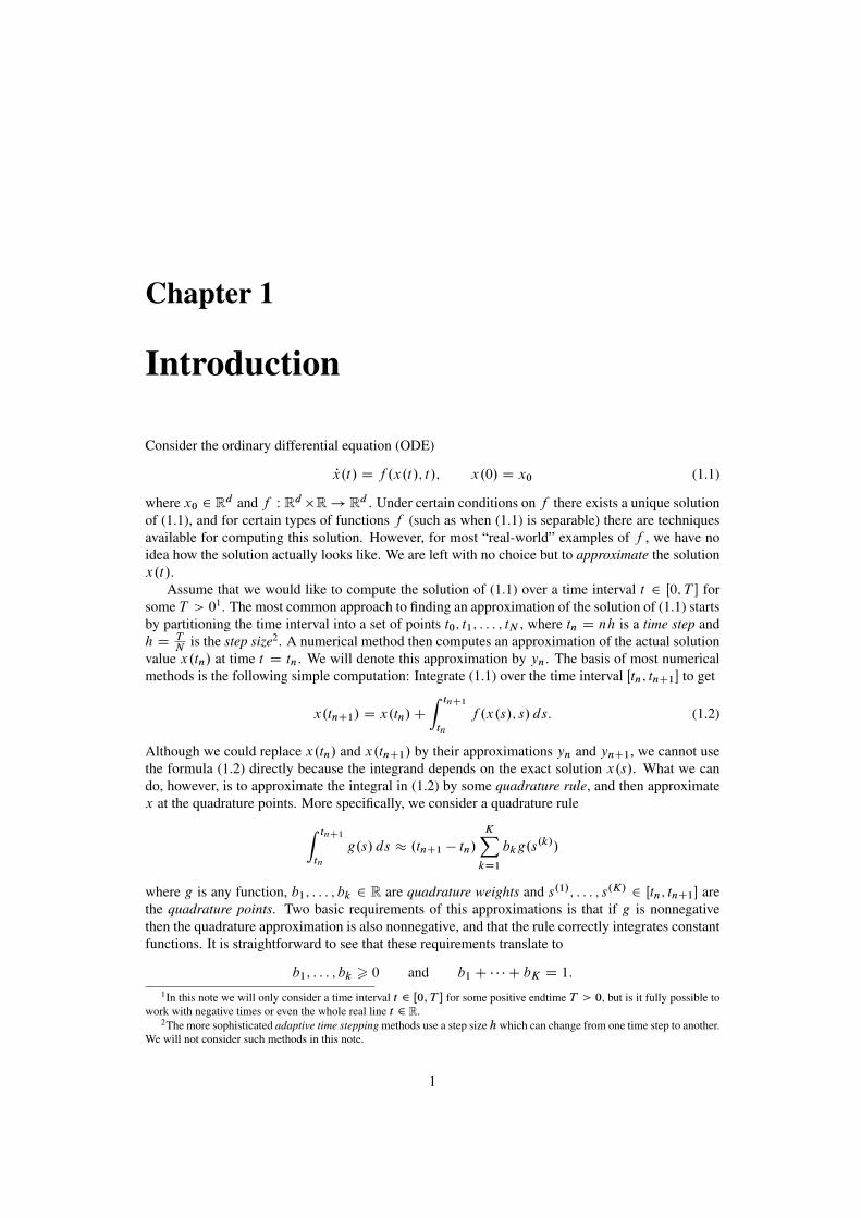
Figure 2.1 show a computation with both schemes using the parameter a D 1 and initial datax0 D 1. While the error in both schemes increase over time, this error decreases as the resolution Nis increased.

4

0 1 2 3 4 5

t

0

50

100

150

200

y

Forward EulerBackward EulerExact solution

0 1 2 3 4 5

t

0

50

100

150

200

y

Forward EulerBackward EulerExact solution

Figure 2.1: Forward and backward Euler computations for the linear, one-dimensional ODE in Ex-ample 2.1 up to time T D 5 using N D 30 (left) and N D 60 (right) time steps.

2.2 Example. Consider an object with massmwhich is hanging from a spring secured to the ceiling.We let q.t/ denote the extension of the spring at time t , and fix the coordinate system so that q D 0is the position at which the object is at rest, and the positive q-axis points vertically down. Hooke’slaw says that the force by the spring on the object is proportional to the extension of the spring:F D �kq.t/, where k > 0 is the stiffness constant of the spring. Applying Newton’s second lawF D ma D m Rq gives us the second-order ODE

m Rq D �kq:

We convert this second-order equation to a system of first-order equations by introducing anotherunknown, the momentum p.t/ D m Pq.t/. This gives us the first-order ODE(

Pp D �kq

Pq D 1mp

(2.3)

We recognize this as a Hamiltonian system with HamiltonianH.p; q/ D k2q2C 1

2mp2, which means

that we can write (Pp D � @H

@q.p; q/

Pq D @H@p.p; q/;

and the function H can be interpreted as the total energy of the system. The ODE (2.3) is oftencalled the harmonic oscillator.

We consider now a numerical method for (2.3). Let us first write the system as

Px D Ax; where x D

p

q

!and A D

0 �k

1=m 0

!:

The forward Euler method (2.1) is then

ynC1 D yn C hAyn D .I2 C hA/yn

where I2 is the identity matrix in R2�2, and the implicit Euler method (2.2) is

ynC1 D yn C hAynC1 ) ynC1 D .I2 � hA/�1yn:

5

0 2 4 6 8 10

t

-3

-2

-1

0

1

2

p

Forward EulerBackward EulerExact solution

0 2 4 6 8 10

t

-4

-3

-2

-1

0

1

2

3

q

Forward EulerBackward EulerExact solution

Figure 2.2: Forward and backward Euler computations for (2.3) using T D 10 and N D 40.

0 2 4 6 8 10

t

0

1

2

3

4

5

6

H(p

,q)

Forward EulerBackward EulerExact solution

Figure 2.3: The total energy H.p; q/ for the computations in Example 2.2.

Figure 2.2 shows the numerically computed solutions for parameter values m D k D 1 and initialdata p D 0, q D 1. The exact solution consists of sinusoidal waves (exercise for the reader!). Ascan be seen in the plots, the explicit Euler method overshoots the exact solutions, while the implicitEuler method undershoots. The same effect is seen in Figure 2.3, where we plot the HamiltonianH.p; q/ as a function of time. Although the total energyH.p; q/ should be constant in time, we seethat the explicit Euler method produces energy, while the implicit Euler dissipates energy over time.We will get back to the issue of Hamiltonian systems and energy preservation in Chapter 5.

2.3 Example. The harmonic oscillator in Example 2.2 is somewhat unrealistic, physically speaking,because there is no friction in the system. We can add friction to our model by modeling it as a forcewhich is proportional to the speed and which acts opposite to the direction of travel:

Ffriction D �c Pq;

where c > 0 is the friction coefficient. Applying Newton’s second law again yields the ODE

m Rq D �kq � c Pq:

Introducing the unknown p D mq, we can convert this second-order ODE to the first-order system

6

0 2 4 6 8 10

t

-1

-0.5

0

0.5

p

Forward EulerBackward EulerExact solution

0 2 4 6 8 10

t

-1

-0.5

0

0.5

1

q

Forward EulerBackward EulerExact solution

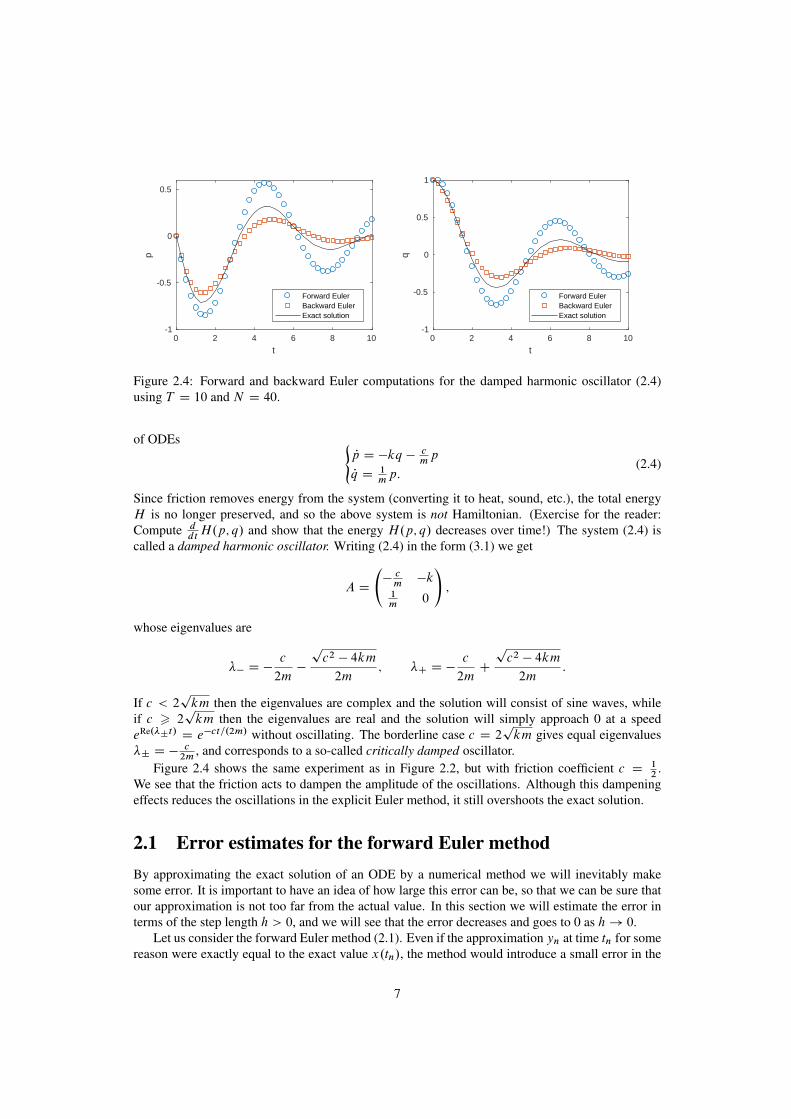
Figure 2.4: Forward and backward Euler computations for the damped harmonic oscillator (2.4)using T D 10 and N D 40.

of ODEs (Pp D �kq � c

mp

Pq D 1mp:

(2.4)

Since friction removes energy from the system (converting it to heat, sound, etc.), the total energyH is no longer preserved, and so the above system is not Hamiltonian. (Exercise for the reader:Compute d

dtH.p; q/ and show that the energy H.p; q/ decreases over time!) The system (2.4) is

called a damped harmonic oscillator. Writing (2.4) in the form (3.1) we get

A D

�cm�k

1m

0

!;

whose eigenvalues are

�� D �c

2m�

pc2 � 4km

2m; �C D �

c

2mC

pc2 � 4km

2m:

If c < 2pkm then the eigenvalues are complex and the solution will consist of sine waves, while

if c > 2pkm then the eigenvalues are real and the solution will simply approach 0 at a speed

eRe.�˙t/ D e�ct=.2m/ without oscillating. The borderline case c D 2pkm gives equal eigenvalues

�˙ D �c2m

, and corresponds to a so-called critically damped oscillator.Figure 2.4 shows the same experiment as in Figure 2.2, but with friction coefficient c D 1

2.

We see that the friction acts to dampen the amplitude of the oscillations. Although this dampeningeffects reduces the oscillations in the explicit Euler method, it still overshoots the exact solution.

2.1 Error estimates for the forward Euler methodBy approximating the exact solution of an ODE by a numerical method we will inevitably makesome error. It is important to have an idea of how large this error can be, so that we can be sure thatour approximation is not too far from the actual value. In this section we will estimate the error interms of the step length h > 0, and we will see that the error decreases and goes to 0 as h! 0.

Let us consider the forward Euler method (2.1). Even if the approximation yn at time tn for somereason were exactly equal to the exact value x.tn/, the method would introduce a small error in the

7

next time step. The local truncation error of a method is precisely the error that the method makesfrom one time step to the next. More specifically, the local truncation error is the quantity

�nC1 WD x.tnC1/ ��x.tn/C hf .x.tn/; tn/

�(2.5)

where x.t/ is the exact solution. More generally, if we have a numerical method of the form

ynC1 D L.yn; tn; h/

for some function L, then the truncation error is defined as �nC1 D x.tnC1/ � L.x.tn/; tn; h/.

2.4 Lemma. The local truncation error for the forward Euler method (2.1) can be bounded by

j�nj 6K.1CM/

2h2

for every n D 1; : : : ; N (where M is the constant in (1.4a)).

Proof. Taylor expand x.t/ around t D tn to get

x.tnC1/ D x.tn/C .tnC1 � tn/dx

dt.tn/C

.tnC1 � tn/2

2

d2x

dt2.s/

for some point s 2 Œtn; tnC1�. Using the facts that tnC1 � tn D h and that x.t/ solves (1.1), we get

x.tnC1/ D x.tn/C hf .x.tn/; tn/Ch2

2

df .x.t/; t/

dt

ˇ̌̌tDs

D x.tn/C hf .x.tn/; tn/Ch2

2

�@f

@x.x.s/; s/

dx

dt.s/C

@f

@t.x.s/; s/

�D x.tn/C hf .x.tn/; tn/C

h2

2

�@f

@x.x.s/; s/f .x.s/; s/C

@f

@t.x.s/; s/

�:

Comparing with the definition of �nC1, we see that

j�nC1j Dh2

2

ˇ̌̌̌@f

@x.x.s/; s/f .x.s/; s/C

@f

@t.x.s/; s/

ˇ̌̌̌6h2

2

�KM CK

�:

We can use the local truncation error to estimate the global error of the method,

en WD x.tn/ � yn: (2.6)

Using (2.1) and (2.5), the error at the next time step can be written as

enC1 D x.tnC1/ � ynC1

D��nC1 C

�x.tn/C hf .x.tn/; tn/

����yn C hf .yn; tn/

�D �nC1 C

�x.tn/ � yn

�C h

�f .x.tn/; tn/ � f .yn; tn/

�D �nC1 C en C h

�f .x.tn/; tn/ � f .yn; tn/

�:

We take absolute values on both sides, apply the triangle inequality and then use the Lipschitzassumption (1.4b):

jenC1j 6 j�nC1j C jenj C hKjx.tn/ � ynj

D j�nC1j C�1C hK

�jenj

8

Applying this inequality to jenj, and then iteratively to jen�1j; jen�2j; : : : ; je1j gives

jenC1j 6 j�nC1j C�1C hK

�jenj

6 j�nC1j C�1C hK

��j�nj C

�1C hK

�jen�1j

�6 : : :

6 j�nC1j C�1C hK

�j�nj C � � � C

�1C hK

�nj�1j C

�1C hK

�nC1je0j

D

nXmD0

�1C hK

�mj�nC1�mj

where the last step follows from the fact that e0 D x.t0/ � y0 D 0. We can now bound the localtruncation terms in the above sum using Lemma 2.4:

jenC1j 6nX

mD0

�1C hK

�mK.1CM/

2h2 D

.1C hK/nC1 � 1

hK

K.1CM/

2h2

D.1CM/

�.1C hK/nC1 � 1

�2

h

where we used the formula for a geometric series. Writing nC 1 D tnC1

hand using the inequality

1C a 6 ea (which is valid for any a 2 R) gives us

jenC1j 6.1CM/

�ehKtnC1=h � 1

�2

h 6.1CM/

�eKT � 1

�2

h

since t0; : : : ; tN 6 T . We have thus proved that there is a constant C > 0 such that jenj 6 Ch forevery n D 1; : : : ; N . We summarize these calculations as follows.

2.5 Lemma. The global error for the forward Euler method (2.1) can be bounded by

jenj 6 Ch

for all n D 0; : : : ; N , where C > 0 is a constant that only depends on f and T .

The technique in the proof of Lemma 2.5 is called Lady Windermere’s Fan, after a play by OscarWilde. The term was most likely coined by Gerhard Wanner in the 1980’s.

Although the constant C in Lemma 2.5 is potentially very large, it is independent of h. Hence,if we would like to know the exact solution up to an error of at most " > 0, then we simply chooseh 6 "

C. (The number " is called the error tolerance.)

2.2 Convergence of the forward Euler methodWe are now close to having proved that the forward Euler method converges to the exact solutionas h ! 0, but to state this precisely we need to specify what we mean by “converges”. What wehave at hand is a sequence of numbers y0; y1; : : : ; yN , one for every value of h D T

N. We need to

interpret these sequences as functions which in some way approximate the function x.t/. To thisend we define the piecewise linear interpolant1

y.t/ D yn Ct � tn

h

�ynC1 � yn

�when t 2 Œtn; tnC1�: (2.7)

1There is no special reason to choose a linear interpolant—we might as well have chosen a piecewise constant or cubicinterpolant. We consider the linear interpolant here because it makes some of the computations easier.

9

This interpolant is continuous, satisfies y.tn/ D yn for every n D 0; 1; : : : ; N , and in-between thetime steps tn; tnC1 it is linear.

Both the exact solution x.t/ and the numerical approximation y.t/ lie in C 0.Œ0; T �;Rd /, thespace consisting of continuous and bounded functions from Œ0; T � into Rd . In particular, their supre-mum norm

kxk1 D supt2Œ0;T �

jx.t/j

is bounded. As is straightforward to check, this is indeed a norm on C 0.Œ0; T �;Rd /. We willmeasure convergence of numerical methods in this norm: If yh.t/ is a sequence of functions inC 0.Œ0; T �;Rd / indexed by h > 0, then we say that yh converges to y, or limh!0 y

h D y, if

limh!0kyh � yk1 D 0:

2.6 Theorem. Let yh.t/ be the piecewise linear interpolant of the forward Euler method using atime step h, and let x.t/ be the exact solution of (1.1). Then there is a constantC > 0, not dependingon h, such that

kx � yhk1 6 Ch:

In particular, the forward Euler method converges to the exact solution x.t/ as h! 0.

Proof. First, note that both x and yh are Lipschitz continuous with Lipschitz constant M . In-deed, the derivative of x is dx

dtD f .x; t/, so jdx

dtj D jf .x; t/j 6 M . For yh we have for every

t 2 Œtn; tnC1� that dyh

dt.t/ D

ynC1�yn

hD f .yn; tn/ (the last step following from (2.1)), so again

jdyh

dt.t/j 6M .

Define the error function eh.t/ D x.t/ � yh.t/. Then eh.tn/ D en for every n D 0; : : : ; N , andeh is Lipschitz continuous with Lipschitz constant at most 2M . Hence, if, say, t 2 .tn; tnC1/ then

jeh.t/j D jeh.t/ � eh.tn/C eh.tn/j 6 je

h.t/ � eh.tn/j C jeh.tn/j

6 2M.t � tn/C Ch 6 .2M C C/h:

The result now follows from the fact that kx � yhk1 D kehk1 D supt2Œ0;T � jeh.t/j.

2.3 Convergence of the implicit Euler methodThe error estimates and the proof of convergence of the implicit Euler method are quite similar tothose of the explicit Euler method, although we have to be more careful since the method is implicit.As before the global error is en WD x.tn/�yn, and the local truncation error is the error that is madeafter a single step in the method. Thus, the local truncation error is

�nC1 WD x.tnC1/ � znC1; where znC1 D x.tn/C hf .znC1; tnC1/:

2.7 Lemma. The local truncation error for the implicit Euler method (2.2) can be bounded by

j�nC1j 6K.M C 1/

2.1 � hK/h2 (2.8)

as long as h < 1K

.

10

Proof. As in the proof of Lemma 2.4 we Taylor expand x.t/, but this time around t D tnC1:

x.tn/ D x.tnC1/C .tn � tnC1/dx

dt.tnC1/C

.tn � tnC1/2

2

d2x

dt2.s/

D x.tnC1/ � hf .x.tnC1/; tnC1/Ch2

2

df .x.t/; t/

dt

ˇ̌̌tDs

for some s 2 Œtn; tnC1�. Using this in �nC1 gives

j�nC1j D

ˇ̌̌̌x.tn/C hf .x.tnC1/; tnC1/ �

h2

2

df .x.t/; t/

dt

ˇ̌̌tDs� x.tn/ � hf .znC1; tnC1/

ˇ̌̌̌6 h

ˇ̌f .x.tnC1/; tnC1/ � f .znC1; tnC1/

ˇ̌Ch2

2

ˇ̌̌̌df .x.t/; t/

dt

ˇ̌̌tDs

ˇ̌̌̌6 hKjx.tnC1/ � znC1j C

h2

2

�KM CK

�6 hKj�nC1j C

h2

2

�KM CK

�:

(Note that, unlike the proof for the forward Euler scheme, the truncation error �nC1 appears in thefinal expression above. This happens because the scheme is implicit.) Solving for j�nC1j gives(2.8).

Once the estimate of the local truncation error (2.8) is in place, the proof of convergence for theimplicit Euler method follows in the same way as for the explicit Euler method. We state the resultsbelow and leave the proofs as exercises for the reader.

2.8 Lemma. Assume that h 6 12K

. Then the global error for the backward Euler method (2.2) canbe bounded by

jenj 6 Ch

for all n D 0; : : : ; N , where C D 3.M C 1/.eKT � 1/ is a constant that only depends on f and T .

2.9 Theorem. Let yh.t/ be the piecewise linear interpolant of the backward Euler method usinga time step h, and let x.t/ be the exact solution of (1.1). Then there is a constant C > 0, onlydepending on f and T , such that

kx � yhk1 6 Ch:

In particular, the backward Euler method converges to the exact solution x.t/ as h! 0.

11

Chapter 3

Stiff problems and linear stability

As shown in the previous chapter, both the explicit and implicit Euler methods converge to the exactsolution as h ! 0, and the error at any time t 2 Œ0; T � can be bounded by Ch for some constantC > 0. Hence, to guarantee that the error is smaller than some error tolerance " > 0, we simplyhave to choose h 6 "

C. There is a catch, though: The constant C is proportional to eKT , where K

is the Lipschitz constant of f , and in many real-world applications this constant can be very large.Such problems are often characterized by a sensitivity to changes in the initial data, or the existenceof features in the solution which change at very different time scales (such as two sine waves withvery different frequency). Problems with some or all of these characteristics are called stiff.

In this chapter we will study stiff linear ODEs

Px D Ax; x.0/ D x0 (3.1)

(forA 2 Rd�d and x0 2 Rd ). Recall that the system (3.1) is linearly stable if the solution is boundedfor all t 2 R, regardless of the choice of x0 2 Rd . Our aim will be to find out how different numericalmethods perform on stiff linear problems, and under what conditions the numerical method is alsolinearly stable.

3.1 One-dimensional problemsTo begin with we consider the linear, one-dimensional ODE

Px D �x; x.0/ D x0 (3.2)

for some � 2 C and x0 2 R. (The reason for allowing complex � will soon be apparent.) Writing� D aC ib for a; b 2 R, the solution of this problem is

x.t/ D e�tx0 D eat�

cos.bt/C i sin.bt/�x0:

Since jx.t/j D eat jx0j, we see that the problem (3.2) is linearly stable if and only if a 6 0:

� 2 C� D˚z 2 C W Re.z/ 6 0

(3.3)

(for otherwise eat will grow towardsC1 as t increases); see Figure 3.1. If jRe.�/j is large then thecorresponding solution x.t/ goes very quickly towards 0 or ˙1, while if jIm.�/j is large then thesolution will oscillate rapidly. We say that the ODE (3.2) is stiff if either of these is the case—thatis, if j�j is large1.

1Of course, “large” depends on your point of view. Here, we mean that T j�j � 1. Since (3.2) states that the rate ofchange of the solution is proportional to j�j, the number T j�j gives an indication of the net change in the solution over thetime interval Œ0; T �.

12

a

b

Figure 3.1: The set C� of all � D aC ib such that (3.2) is linearly stable (in blue).

3.1 Example. Consider the stiff ODE (3.2) with � D �100 and x0 D 1, whose solution is x.t/ De�100t . Figure 3.2(a)–(c) shows computations with the explicit Euler method for three differentchoices of h. On the coarsest mesh (Figure 3.2(a)) the method jumps erratically between positiveand negative values and reaches values of 107. Increasing the resolution (Figure 3.2(b)) improvesthe solution, but still shows some initial oscillations. Only on the finest resolution (Figure 3.2(c)) isthe numerical solution qualitatively correct.

Figure 3.2(d)–(f) shows the same computation but with the implicit Euler method. Unlike theexplicit method, the implicit method shows qualitatively correct behavior on all the three resolutions.The error estimate for the implicit method, Lemma 2.8, bounds the error by .M C 1/.eKT � 1/h,and since K D 100 and T D 1, the term eKT � 1043 is huge. Thus, the implicit method providesa reasonable, qualitatively correct solution for step sizes h much larger than what the error estimateseems to require.

0 0.2 0.4 0.6 0.8 1

t

-1

-0.5

0

0.5

1

1.5

y

10 7

Forward EulerExact solution

(a) h D 140

0 0.2 0.4 0.6 0.8 1

t

-0.4

-0.2

0

0.2

0.4

0.6

0.8

1

y

Forward EulerExact solution

(b) h D 180

0 0.2 0.4 0.6 0.8 1

t

0

0.2

0.4

0.6

0.8

1

y

Forward EulerExact solution

(c) h D 1120

0 0.2 0.4 0.6 0.8 1

t

0

0.2

0.4

0.6

0.8

1

y

Backward EulerExact solution

(d) h D 140

0 0.2 0.4 0.6 0.8 1

t

0

0.2

0.4

0.6

0.8

1

y

Backward EulerExact solution

(e) h D 180

0 0.2 0.4 0.6 0.8 1

t

0

0.2

0.4

0.6

0.8

1

y

Backward EulerExact solution

(f) h D 1120

Figure 3.2: Forward Euler (top row) and backward Euler (bottom row) for the stiff problem inExample 3.1 up to time T D 1.

13

a

b

(a) Explicit Euler

a

b

(b) Implicit Euler

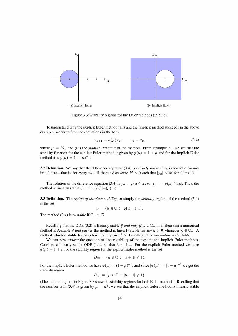
Figure 3.3: Stability regions for the Euler methods (in blue).

To understand why the explicit Euler method fails and the implicit method succeeds in the aboveexample, we write first both equations in the form

ynC1 D '.�/yn; y0 D x0; (3.4)

where � D h�, and ' is the stability function of the method. From Example 2.1 we see that thestability function for the explicit Euler method is given by '.�/ D 1C � and for the implicit Eulermethod it is '.�/ D .1 � �/�1.

3.2 Definition. We say that the difference equation (3.4) is linearly stable if yn is bounded for anyinitial data—that is, for every x0 2 R there exists some M > 0 such that jynj 6M for all n 2 N.

The solution of the difference equation (3.4) is yn D '.�/nx0, so jynj D j'.�/jnjx0j. Thus, themethod is linearly stable if and only if j'.�/j 6 1.

3.3 Definition. The region of absolute stability, or simply the stability region, of the method (3.4)is the set

D D˚� 2 C W j'.�/j 6 1

:

The method (3.4) is A-stable if C� � D.

Recalling that the ODE (3.2) is linearly stable if and only if � 2 C�, it is clear that a numericalmethod is A-stable if and only if the method is linearly stable for any h > 0 whenever � 2 C�. Amethod which is stable for any choice of step size h > 0 is often called unconditionally stable.

We can now answer the question of linear stability of the explicit and implicit Euler methods.Consider a linearly stable ODE (1.1), so that � 2 C�. For the explicit Euler method we have'.�/ D 1C �, so the stability region for the explicit Euler method is the set

DFE D˚� 2 C W j�C 1j 6 1g:

For the implicit Euler method we have '.�/ D .1��/�1, and since j'.�/j D j1��j�1 we get thestability region

DBE D˚� 2 C W j� � 1j > 1g:

(The colored regions in Figure 3.3 show the stability regions for both Euler methods.) Recalling thatthe number � in (3.4) is given by � D h�, we see that the implicit Euler method is linearly stable

14

for any h > 0, while the explicit Euler method is linearly stable only for small values of h, whenjh�C 1j 6 1. Hence, the implicit Euler method is A-stable, while the explicit Euler method is onlyconditionally stable—it is only stable for certain (small) values of the step size h.

If � is a real, negative number then the explicit Euler method is linearly stable for h� 2 Œ�2; 0�,or h 6 2

j�j. In Example 3.1 we had � D �100 so the value h D 1

40in Figure 3.2(a) lies outside the

region of linear stability.

3.2 Multi-dimensional problemsWe consider next a general d -dimensional linear system (3.1). For the sake of simplicity we assumethat A is diagonalizable and we let �1; : : : ; �d 2 C be the eigenvalues and v1; : : : ; vd 2 Cd thecorresponding eigenvectors of A. The exact solution of (3.1) is then

x.t/ D ˛1e�1tv1 C � � � C ˛de

�d tvd (3.5)

where ˛1; : : : ; ˛d 2 C are such that ˛1v1 C � � � C ˛dvd D x0. If we write �k D ak C ibk fork D 1; : : : ; d then the contribution ˛ke�k tvk from the kth eigenpair consists of a scaling eak t anda rotation with frequency bk . Thus, if the numbers a1; : : : ; ad and b1; : : : ; bd are of very differentmagnitude, then the formula (3.5) is a sum of terms which “live” on several different time scales.We say that the linear system (3.1) is stiff if the real and imaginary parts of the eigenvalues of Adiffer by several orders of magnitude, or if they are much larger in magnitude than 1

T. Note that in

the scalar case d D 1, this definition is equivalent to the one given in Section 3.1.Recall that the linear system (3.1) is spectrally stable if Re.�k/ 2 C� for all eigenvalues

�1; : : : ; �d , and is linearly stable if all solutions are bounded for all t . It can be shown that when Ais diagonalizable, these two notions of stability are equivalent.

3.4 Example. Consider the damped harmonic oscillator from Example 2.3, but assume that thespring is relatively stiff2, say, k D 10. From the computation in Example 2.3 we get eigenvalues

�˙ D �14˙

q�10C 1

16� �

14˙3:15i , so the solution will contain a dampening term e�t=4 as well

as sine waves with a period of approximately 2�3:15� 2. In particular, the real parts Re.�˙/ D �14

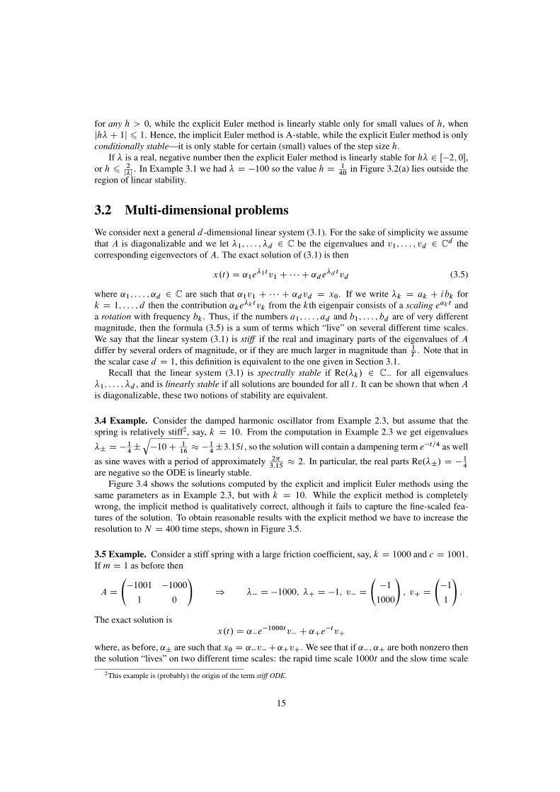
are negative so the ODE is linearly stable.Figure 3.4 shows the solutions computed by the explicit and implicit Euler methods using the

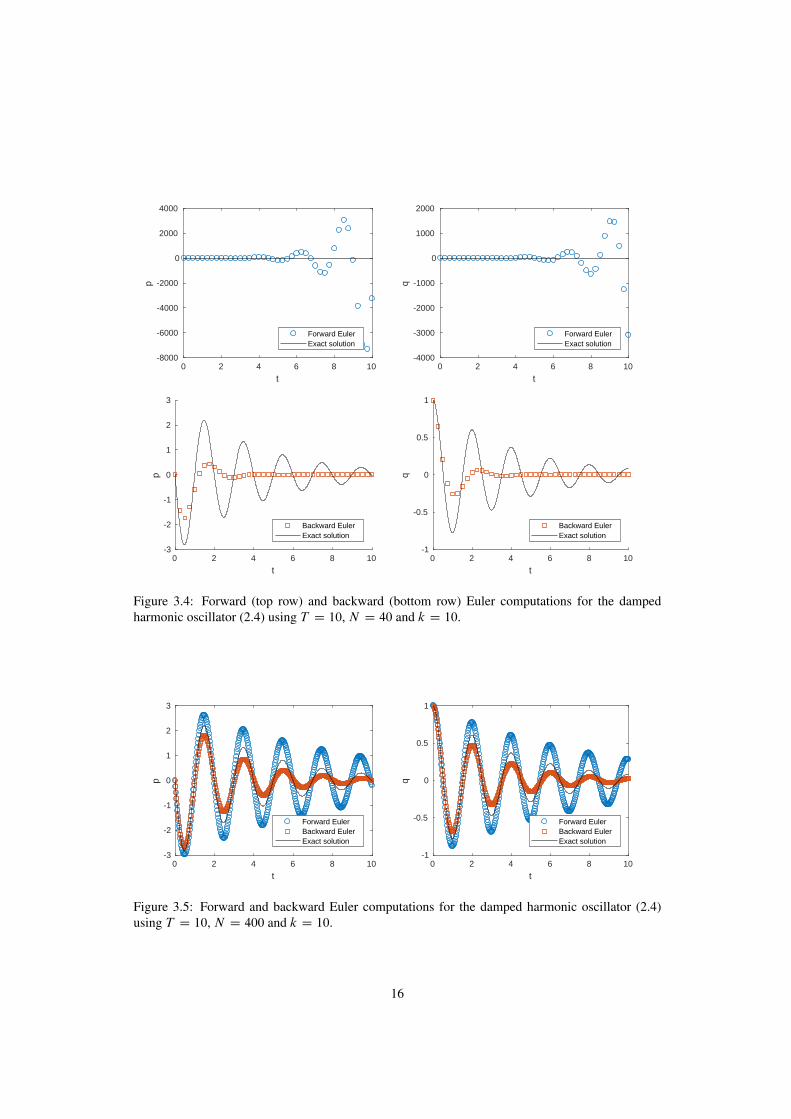
same parameters as in Example 2.3, but with k D 10. While the explicit method is completelywrong, the implicit method is qualitatively correct, although it fails to capture the fine-scaled fea-tures of the solution. To obtain reasonable results with the explicit method we have to increase theresolution to N D 400 time steps, shown in Figure 3.5.

3.5 Example. Consider a stiff spring with a large friction coefficient, say, k D 1000 and c D 1001.If m D 1 as before then

A D

�1001 �1000

1 0

!) �� D �1000; �C D �1; v� D

�1

1000

!; vC D

�1

1

!:

The exact solution isx.t/ D ˛�e

�1000tv� C ˛Ce�tvC

where, as before, ˛˙ are such that x0 D ˛�v�C˛CvC. We see that if ˛�; ˛C are both nonzero thenthe solution “lives” on two different time scales: the rapid time scale 1000t and the slow time scale

2This example is (probably) the origin of the term stiff ODE.

15

0 2 4 6 8 10

t

-8000

-6000

-4000

-2000

0

2000

4000

p

Forward EulerExact solution

0 2 4 6 8 10

t

-4000

-3000

-2000

-1000

0

1000

2000

q

Forward EulerExact solution

0 2 4 6 8 10

t

-3

-2

-1

0

1

2

3

p

Backward EulerExact solution

0 2 4 6 8 10

t

-1

-0.5

0

0.5

1q

Backward EulerExact solution

Figure 3.4: Forward (top row) and backward (bottom row) Euler computations for the dampedharmonic oscillator (2.4) using T D 10, N D 40 and k D 10.

0 2 4 6 8 10

t

-3

-2

-1

0

1

2

3

p

Forward EulerBackward EulerExact solution

0 2 4 6 8 10

t

-1

-0.5

0

0.5

1

q

Forward EulerBackward EulerExact solution

Figure 3.5: Forward and backward Euler computations for the damped harmonic oscillator (2.4)using T D 10, N D 400 and k D 10.

16

0 2 4 6 8 10

t

-1

-0.8

-0.6

-0.4

-0.2

0

0.2

p

Forward EulerExact solution

0 2 4 6 8 10

t

0

0.2

0.4

0.6

0.8

1

q

Forward EulerExact solution

0 2 4 6 8 10

t

-1

-0.8

-0.6

-0.4

-0.2

0

p

Backward EulerExact solution

0 2 4 6 8 10

t

0

0.2

0.4

0.6

0.8

1

q

Backward EulerExact solution

Figure 3.6: Forward (top row) and backward (bottom row) Euler computations for the dampedharmonic oscillator (2.4) using T D 10, N D 40, k D 1000 and c D 1001.

t . If ˛� D 0, however, the solution is simply x.t/ D ˛Ce�tvC, and it might seem that the problemis non-stiff. Figure 3.6 shows the computed solution when x0 D vC. The solution should convergeto zero at the moderate pace e�t , but while the implicit method computes the correct solution, theexplicit method suddenly jumps at around t � 9, and quickly reaches values of around 108.

From the two examples above we can deduce two things. First, the presence of moderately largeeigenvalues puts strict restrictions on the step size for the explicit (but not the implicit) Euler method.Second, even if x0 is such that the solution does not “see” the large eigenvalues (that is, the solutionlies entirely in the eigenspace corresponding to small eigenvalues), small round-off errors mightcause instabilities in the explicit (but not the implicit) Euler method.

To study the linear stability of the explicit and implicit Euler methods we first perform a changeof variables for the equation (3.1): If u.t/ D P�1x.t/ (where P is the matrix of eigenvectors) thenu solves the ordinary differential equation

Pu D ƒu; u.0/ D P�1x0;

whose solution is u.t/ D etƒP�1x0. Letting yn be the forward Euler approximation of (3.1), thesequence wn D P�1yn solves the difference equation

wnC1 D wn C hƒwn D .Id C hƒ/wn; w0 D P�1x0:

Just as for the differential equation, we have decoupled the components of yn, yielding d scalar

17

difference equationswknC1 D .1C h�k/w

kn : (3.6)

Since yn stays bounded if and only if w1n; : : : ; wdn stay bounded, we see that the forward Euler

method for (3.1) is linearly stable if and only if the forward Euler method (3.6) for each of theunknowns u1.t/; : : : ; ud .t/ is linearly stable. In particular, the forward Euler method for (3.1) islinearly stable if and only if

j1C h�kj 6 1 8 k D 1; : : : ; d:

In a similar fashion we find that the implicit Euler method is linearly stable if and only if

j1 � h�kj > 1 8 k D 1; : : : ; d:

In particular, if (3.1) is linearly stable, that is, �1; : : : ; �d 2 C�, then the implicit Euler method islinearly stable for any h > 0.

18

Chapter 4

Runge–Kutta methods

While the explicit and implicit Euler methods work just fine in a large number of applications, theyonly converge at a rate of O.h/. This is not an issue for the relatively simple problems consideredin the previous chapters, but the amount of work required to get below a given error tolerance " > 0could become insurmountable if, for instance:

� the number of dimensions d is large

� the end time T is large

� the ODE is stiff

� the error tolerance " is small

� the computational resources available are limited.

(While the last point is less of a problem today, it was a big factor when many of the methodsdiscussed here were developed several decades ago.) This motivates developing numerical methodswhich converge at a speed O.hp/ for p > 1.

Many of the ideas developed in Chapter 2 will carry over to the methods developed in thischapter. Most importantly, the principle of Lady Windermere’s Fan—the conversion of a truncationerror estimate to a global error estimate—still applies. Let us consider a (possibly implicit) numericalmethod for (1.1) of the form

ynC1 D yn C hˆ�yn; ynC1; tn; h

�: (4.1)

Then the local truncation error of the method is defined as

�nC1 WD x.tnC1/ � znC1; where znC1 D x.tn/C hˆ�x.tn/; znC1; tn; h

�;

which can be interpreted as the error that the method makes from one time step to the next. Theglobal error of the method is en WD x.tn/ � yn.

4.1 Lemma (Lady Windermere’s Fan). Assume that the function ˆ in (4.1) is Lipschitz continuousin the two first variables. Assume moreover that j�nj 6 ChpC1 for some p 2 N and some C > 0

which is independent of h. Then jenj 6 QChp .

19

4.1 Second-order methodsAs explained in Chapter 1 we can write

x.tnC1/ D x.tn/C

Z tnC1

tn

f .x.s/; s/ ds: (4.2)

The above integral depends on the exact solution and hence must be approximated by some quadra-ture rule, that is, some function ˆ such that

x.tnC1/ � x.tn/ D

Z tnC1

tn

f .x.s/; s/ ds � hˆ�x.tn/; x.tnC1/; tn; h

�:

Assume that the quadrature rule ˆ is pth order accurate, so that

hˆ�x.tn/; x.tnC1/; tn; h

�D

Z tnC1

tn

f .x.s/; s/ ds CO.hpC1/ (4.3)

for some p 2 N, and let us assume that ˆ is Lipschitz continuous,ˇ̌ˆ�x1; x2; t; h

��ˆ

�y1; y2; t; h

�ˇ̌6 Lˆ

�jy1 � x1j C jy2 � x2j

�8 x1; x2; y1; y2 (4.4)

for some Lˆ > 0. If we use ˆ in the numerical method (4.1) then the truncation error will be

j�nC1j Dˇ̌x.tnC1/ � znC1

ˇ̌Dˇ̌x.tnC1/ �

�x.tn/C hˆ

�x.tn/; znC1; tn; h

��ˇ̌D

ˇ̌̌̌Z tnC1

tn

f .x.s/; s/ ds � hˆ�x.tn/; znC1; tn; h

�ˇ̌̌̌(by (4.2))

6

ˇ̌̌̌Z tnC1

tn

f .x.s/; s/ ds � hˆ�x.tn/; x.tnC1/; tn; h

�ˇ̌̌̌C h

ˇ̌ˆ�x.tn/; x.tnC1/; tn; h

��ˆ

�x.tn/; znC1; tn; h

�ˇ̌(triangle inequality)

6 ChpC1 C hLˆˇ̌x.tnC1/ � znC1

ˇ̌(by (4.3) and (4.4))

D ChpC1 C hj�nC1j

Solving for �nC1 gives

j�nC1j 6C

1 � hLˆhpC1:

If, say, h 6 12Lˆ

then the term in front of hpC1 is less than 2C . Hence, applying Lemma 4.1 we geta global error of en D O.hp/.

4.1.1 The Crank–Nicholson methodThe simplest quadrature rule which is more than first-order accurate is perhaps the trapezoidal rule,Z tnC1

tn

g.s/ ds Dh

2

�g.tn/C g.tnC1/

�CO.h3/:

Inserting g.s/ D f .x.s/; s/, we obtain the approximation

x.tnC1/ D x.tn/Ch

2

�f .x.tn/; tn/C f .x.tnC1/; tnC1/

�CO.h3/: (4.5)

20

The resulting numerical method can be written in the following form:8̂<̂:k1 D f .yn; tn/

k2 D f .ynC1; tnC1/

ynC1 D yn Ch2.k1 C k2/:

(4.6)

This is the Crank–Nicholson method. Note that this method is implicit, since k2 depends on ynC1and vice versa.

4.1.2 Heun’s methodThe Crank–Nicholson method (4.6) is implicit and can therefore be difficult to compute with if f isnonlinear. The troublesome term is f .x.tnC1/; tnC1/ in the trapezoidal rule (4.5). A common trickis to replace the exact value x.tnC1/ by an approximate value, such as the forward Euler computation

x.tnC1/ D x.tn/C hf .x.tn/; tn/CO.h2/:

Using this in the right-hand side of (4.5) gives (denoting xn D x.tn/ and xnC1 D x.tnC1/)

xnC1 D xn Ch

2

�f .xn; tn/C f .xnC1; tnC1/

�CO.h3/

D xn Ch

2

�f .xn; tn/C f

�xn C hf .xn; tn/CO.h

2/; tnC1

��CO.h3/

D xn Ch

2

�f .xn; tn/C f

�xn C hf .xn; tn/; tnC1

�CO.h2/

�CO.h3/

D xn Ch

2

�f .xn; tn/C f

�xn C hf .xn; tn/; tnC1

��CO.h3/:

(In the third line we have used the Lipschitz continuity of f to take the O.h2/ term out of f .) Theresulting second-order, explicit method can be written as8̂<̂

:k1 D f .yn; tn/

k2 D f .yn C hk1; tn C h/

ynC1 D yn Ch2.k1 C k2/:

(4.7)

This is Heun’s method or the improved Euler method.

4.1.3 The modified Euler methodAnother third-order accurate quadrature is the midpoint rule,Z tnC1

tn

g.s/ ds D hg.tnC1=2/CO.h3/;

where tnC1=2 DtnCtnC1

2. Inserting g.s/ D f .x.s/; s/ gives the approximation

x.tnC1/ � x.tn/ D f .x.tnC1=2/; tnC1=2/CO.h3/:

We can use the same trick as for Heun’s method to approximate the midpoint value x.tnC1=2/ withthe forward Euler method:

x.tnC1=2/ D x.tn/Ch

2f .x.tn/; tn/CO.h

2/:

21

We find that (denoting xn D x.tn/ and xnC1=2 D x.tnC1=2/)Z tnC1

tn

f .x.s/; s/ ds D hf�xnC1=2; tnC1=2

�CO.h3/

D hf�xn C

h2f .xn; tn/CO.h

2/; tnC1=2

�CO.h3/

D hf�xn C

h2f .xn; tn/; tnC1=2

�C hO.h2/CO.h3/

D hf�xn C

h2f .xn; tn/; tnC1=2

�CO.h3/:

We can conclude that if we define

ˆ.yn; tn; h/ D f�yn C

h2f .yn; tn/; tnC1=2

�then the method (4.1) has a global error ofO.h2/. We can write out the resulting method as follows:8̂<̂

:k1 D f .yn; tn/

k2 D f�yn C

h2k1; tn C

h2

�ynC1 D yn C hk2:

(4.8)

This method is often called the modified Euler method.

4.2 Butcher tableausThe observant reader will have noticed that we have written all of the second-order accurate methods(4.6), (4.7), (4.8) in a similar manner. In fact, all three methods can be written in the following form:8̂̂<̂

:̂k1 D f

�yn C h

P2jD1a1jkj ; tn C c1h

�k2 D f

�yn C h

P2jD1a2jkj ; tn C c2h

�ynC1 D yn C h

P2iD1biki

(4.9)

for some coefficients aij , bj and cj . These coefficients can be neatly collected in what is called aButcher tableau1

c1 a11 a12

c2 a21 a22

b1 b2

The Butcher tableaus of the second-order methods in Section 4.1 are as follows:

0 0 0

1 1=2 1=2

1=2 1=2

Crank–Nicholson

0 0 0

1 1 0

1=2 1=2

Heun’s method

0 0 0

1=2 1=2 0

0 1

Modified Euler

1After the New Zealand mathematician John Charles Butcher (1933–).

22

These methods are examples of two-stage Runge–Kutta methods2. More generally, an s-stageRunge–Kutta method is a method of the form8̂̂̂̂

<̂̂ˆ̂̂̂:k1 D f

�yn C h

PsjD1a1jkj ; tn C c1h

�:::

ks D f�yn C h

PsjD1asjkj ; tn C csh

�ynC1 D yn C h

PsiD1biki

(4.10)

where aij , bj , cj are coefficients that can be collected in a Butcher tableau:

c1 a11 � � � a1s:::

:::: : :

:::

cs as1 � � � ass

b1 � � � bs

or even more compactly,

c A

b>

where A D�aij�si;jD1

is the Runge–Kutta matrix, b D�bi�siD1

is the vector of Runge–Kutta weights

and c D�ci�siD1

is the vector of Runge–Kutta nodes.From (4.10) we see that if aij D 0 for every j > i then ki only depends on preceding values

k1; : : : ; ki�1, which implies that the method is explicit. Conversely, if aij ¤ 0 for some j > i thenthe expression for ki depends either on ki itself or some unknown, yet to be computed value kj , andhence the method is implicit. Hence, by checking whether the diagonal and upper-diagonal entriesof the Runge–Kutta matrix are zero, we quickly determine if the method is explicit or implicit. Inthis way we easily see that the Crank–Nicholson method is implicit, while Heun’s and the modifiedEuler methods are explicit.

4.2 Example. The explicit and implicit Euler methods are one-stage Runge–Kutta methods withButcher tableaus

0 0

1and

1 1

1

respectively.

4.3 Example. Runge and Kutta’s original method (often simply referred to as the Runge–Kuttamethod) is the fourth-order accurate, four-stage method with Butcher tableau

0

1=2 1=2

1=2 0 1=2

1 0 0 11=6 1=3 1=3 1=6

(here a missing entry means 0).2After the German mathematicians Carl David Tolmé Runge (1856–1927) and Martin Wilhelm Kutta (1867–1944).

23

4.3 Consistency and order of accuracyGiven a Runge–Kutta method, how do we determine its order? How do we construct a method whichis, say, pth order accurate? How many stages s are required for a pth order explicit Runge–Kuttamethod? The first question is actually not so easy to answer; the second question requires someadvanced graph theory; and the third question is an unsolved problem! In this section we will onlydevelop some rudimentary ideas and basic consistency requirements, and we refer to more thoroughtreatises such as [3, Chapter 3] or [1] for further details.

The basic idea to deriving a pth order Runge–Kutta method is the same as for the second-order methods in Section 4.1. Begin by applying a quadrature rule (such as Gauss quadrature) toapproximate

x.tnC1/ D x.tn/C

Z tnC1

tn

f�x.s/; s

�ds

� x.tn/C h

sXiD1

bif�x�tn C hci

�; tn C hci

�where tnChci 2 Œtn; tnC1� are the quadrature points and bi the quadrature weights. A basic require-ment of the quadrature weights is that

sXiD1

bi D 1: (4.11)

This guarantees that the quadrature rule is exact whenever f is constant, which is a necessary re-quirement for the method to be at least first-order accurate.

Let yn and ynC1 be approximations of x.tn/ and x.tnC1/, respectively, and let y.i/n approximatex�tn C hci

�. Then

ynC1 D yn C h

sXiD1

bif�y.i/n ; tn C hci

�(4.12a)

gives an approximation of x.tnC1/. Using the fact that

x�tn C hci

�D x.tn/C

Z tnChci

tn

f�x.s/; s

�ds

we can express y.i/n by approximating the above integral using another quadrature rule. Since usingquadrature points other than tn C hc1; : : : ; tn C hcs would introduce new, unknown values of x, westick to these quadrature points:

y.i/n D yn C hci

sXjD1

Qaijf�y.j /n ; tn C hcj

�(4.12b)

(the factor hci is the length of the integration domain), where Qai1; : : : ; Qais are the quadrature weightsto compute y.i/n . Just as in (4.11), a basic consistency requirement for the quadrature weights Qaij isPsjD1 Qaij D 1. Defining aij D ci Qaij , this requirement translates to

sXjD1

aij D ci for every i D 1; : : : ; s: (4.13)

Putting together (4.12a) and (4.12b) gives exactly the Runge–Kutta method (4.10). Note that all ofthe Butcher tableaus given in Section 4.2 satisfy the consistency requirements (4.11) and (4.13).

24

So what is the order of accuracy of a given Runge–Kutta method? Unfortunately there is nostraightforward method to answer this question. One approach consist of Taylor expanding f andx around each quadrature point, but this quickly becomes too messy for any order p greater than 2.For a systematic (but quite technical) method of using graphs to express Taylor expansions, see [1].

For explicit Runge–Kutta methods it is known that one needs at least s D p stages to obtain pthorder accuracy. In fact, if p > 5 then one needs s > p C 1 stages, and this trend continues forlarger values of p: The number of stages s grows faster than p. For implicit Runge–Kutta methods,on the other hand, it is known that the order of accuracy of an s-stage method is at most p D 2s,and for every s 2 N there is in fact a unique 2s-order accurate, s-stage Runge–Kutta method. (Thisis analogous to the uniqueness of the s-point, .2s C 1/th order accurate Gauss quadrature rule.)Thus, there is a tradeoff here: An implicit, s-stage method is potentially much more accurate than anexplicit s-stage method, but on the other hand, implicit methods require solving implicit equationsand are hence much more computationally demanding.

4.4 Linear stability of Runge–Kutta methodsIn this section we investigate the linear stability of Runge–Kutta methods. We will see that for thesemethods, the general rule of thumb of stability still holds: implicit methods are stable regardless ofthe timestep h, while explicit methods are only stable for sufficiently small h.

Recall from Chapter 3 that a numerical method is linearly stable if the computed solution staysbounded for all times when solving the linear ODE

Px D �x

for some � 2 C. We insert the choice f .x/ D �x into the general form of a Runge–Kutta method(4.10) to get 8̂̂̂̂

<̂ˆ̂̂:k1 D �yn C �h

PsjD1a1jkj

:::

ks D �yn C �hPsjD1asjkj

ynC1 D yn C hPsiD1biki :

(4.14)

We can write the above in matrix notation:

k D 1�yn C �hAk; ynC1 D yn C hb>k

where 1 and k are the vectors 1 D�1 1 � � � 1

�> and k D�k1 k2 � � � ks

�>, and b is the vectorof Runge–Kutta weights. Solving the above for k gives k D .I � �A/�11�yn, where we denote� D �h, as before. This gives ynC1 D yn'.�/, where '.�/ D 1C�b>.I ��A/�11 is the stabilityfunction for the Runge–Kutta method (4.14) (see Section 3.1). We can simplify this expression evenfurther:

4.4 Lemma. The stability function for the s-step Runge–Kutta method (4.14) is

'.�/ Ddet

�I � �AC �1b>

�det

�I � �A

� : (4.15)

The proof of the above lemma is outside the scope of these notes, but the idea is to use Cramer’srule to invert the matrix I ��A (see [2, Section IV.3]). As an exercise, try to use the formula (4.15)

25

to compute the stability functions for the explicit and implicit Euler methods (see Example 4.2) andsee if you get the same results as in Chapter 3.

Let us first assume that the method in question is explicit, so that aij D 0 for all j > i . ThenI � �A is a lower-triangular matrix with ones along the diagonal, so det

�I � �A

�D 1. The

numerator in (4.15) is the determinant of an s � s matrix, so it follows that the stability function foran explicit Runge–Kutta method is an sth order polynomial,

'.�/ D 1C d1�C d2�2C � � � C ds�

s

for some coefficients d1; : : : ; ds 2 R. The classical result of Liouville (see any textbook on complexanalysis) states that every non-constant polynomial is unbounded. Hence, the stability region

D D˚� 2 C W j'.�/j 6 1

of any explicit Runge–Kutta method is a bounded set, and in particular, the method is only stable forcertain values of h.

If the Runge–Kutta method is in implicit then it is generally not the case that det�I ��A

�equals

1; instead it will be some sth order polynomial of �. Consequently, the stability function (4.15) isa rational polynomial (that is, one polynomial divided by another) which in many cases is boundedfor any value of �.

Figure 4.1 shows the stability functions and stability regions for the four different Runge–Kuttamethods encountered in this chapter. We see that the stability functions of the explicit methods(Figures (b)–(d)) are polynomials, and that their stability regions are bounded sets. Hence, if theproblem is stiff—that is, if j�j � 1—then the step size h must be very small in order to get a stablemethod. On the other hand, the stability function of the implicit Crank–Nicholson method (Figure(a)) is a rational polynomial, and the stability region is D D C�. It follows that the Crank–Nicholsonmethod is A-stable.

26

'.�/ D 2C�2��

(a) Crank–Nicholson

'.�/ D 1C �C �2

2

(b) Heun’s method

'.�/ D 1C �C �2

2

(c) Modified Euler

'.�/ D 1C �C �2

2C

�3

6C

�4

24

(d) The classic R–K 4 method

Figure 4.1: Stability functions and stability regions (in blue) for different Runge–Kutta methods.

27

Chapter 5

Symplectic methods

Recall that a Hamiltonian system is an ordinary differential equation which can be written in theform (

Pp D � @H@q.p; q/

Pq D @H@p.p; q/

(5.1)

for some function H D H.p; q/. For simplicity we will assume in this chapter that the unknownfunctions p; q are scalar-valued, but emphasize that everything in this chapter can be generalized tovector-valued unknowns.

We have already seen one example of a Hamiltonian system in Example 2.2, the harmonic oscil-lator. Other examples of Hamiltonian systems include the equations of motion of a planetary systemor of particles in a particle accelerator. In many applications it is important to be able to solve thesesystems very accurately for a long time. For instance, an astrophysicist could ask whether an aster-oid in our solar system will collide with Earth sometime during the next fifty years; any small errorin the computation might give a false negative. Or a particle physicist at CERN could ask whethera beam of particles will make it through the Large Hadron Collider particle accelerator over thenext few seconds; the particles pass through each of the 1232 magnets in the the 27 km long tunnelmore than 11.000 times per second, so any inaccuracies will quickly multiply and give an incorrectanswer.

An easy solution would be to use a high-order accurate numerical method, such as a Runge–Kutta method. But very high-dimensional or long-time problems might still be too computationallyexpensive for the desired accuracy, even with a high-order accurate method.

5.1 Example. As we saw in Example 2.2, the explicit and implicit Euler methods were quite in-accurate when simulating the harmonic oscillator (cf. Figure 2.2). Figure 5.1(a) shows the sameproblem computed with Heun’s method. It’s clear that the second-order method gives a much betterapproximation. But what if we want to compute for a longer time, say, until T D 200? As shownin Figure 5.1(b), the method slowly, but surely starts to overestimate the amplitude of the oscillator,and at the end of the simulation the error is of the order of 1.

By simply using a higher-order accurate method we are treating the ODE (5.1) just like any otherODE. As we will see in this chapter, we will gain much more in accuracy if we take advantage ofthe very special Hamiltonian structure (5.1).

28

0 2 4 6 8 10

t

-2

-1

0

1

2

p

Forward EulerBackward EulerHeun's methodExact solution

(a) T D 10

0 50 100 150 200

t

-2

-1

0

1

2

p

Heun's methodExact solution

(b) T D 200

Figure 5.1: The p component in the harmonic oscillator (2.3), computed with Heun’s method.

5.1 Symplectic mapsLet x D .p q/> be the vector of unknowns and let ' be the flow of the ODE (5.1), so that 't .x/solves (5.1) with initial data x 2 R2. In this section we will see that, in addition to preserving theHamiltonian H.'t .x// over time, the flow ' has the property of being area preserving.

If x1 D .p1 q1/> and x2 D .p2 q2/

> are given vectors then the area of the parallelogramspanned by x1 and x2 is given by

!.x1; x2/ D p1q2 � p2q1 D x>1 Jx2; where J D

0 1

�1 0

!:

Let now g W R2 ! R2 be some given function, and assume for the moment that g is linear, so thatg.x/ D Ax for some A 2 R2�2. We say that g (or A) is symplectic if it preserves the area of allsuch paralellograms, that is, if

!�g.x1/; g.x2/

�D !.x1; x2/ 8 x1; x2 2 R:

Inserting g.x/ D Ax, it is not hard to see that g is symplectic if and only if

A>JA D J: (5.2)

5.2 Exercise. Let

A D

cos � � sin �

sin � cos �

!; B D

2 0

0 1=2

!; C D

2 0

0 2

!for some � 2 Œ0; 2�/. Show that A and B are symplectic, and that C is not.

Let now g W R2 ! R2 be an arbitrary, possibly nonlinear function. Noting that the matrix Aabove is the Jacobian of g, we say that g is symplectic if the identity (5.2) is true for the matrixA D rg.x/, for every x 2 R2. Although we will not go into details here, it is possible to use toolsfrom differential geometry to show that g being symplectic is the same as saying that g preserves

29

area—that is, if � � R2 is some bounded set, then � and g.�/ D fg.x/ W x 2 �g have the samearea.

We now investigate the flow 't .x/ of the Hamiltonian system (5.1). First, observe that we canwrite the system (5.1) as

Px D �JrH.x/ (5.3)

where rH.p; q/ D�@H@p.p; q/ @H

@q.p; q/

�>.

5.3 Theorem (Poincaré, 1899). Let ' be the flow of the Hamiltonian system (5.1). Then for everyt 2 R, the function 't .x/ is symplectic.

Proof. We need to check that for every fixed time t 2 R and x 2 R2, the matrix A D r't .x/satisfies (5.2). If t D 0 then 't .x/ D x, so A D I , which clearly satisfies (5.2). For a general t 2 Rwe see from (5.3) that

d

dtr't .x/ D r

�ddt't .x/

�D �r

�JrH.'t .x//

�D �Jr2H.'t .x//r't .x/:

(Here, r2H is the Hessian matrix of H , consisting of all second-order partial derivatives of H .)Hence, if A D r't .x/ then

d

dt

�A>JA

�D

d

dt

�r't .x/

>Jr't .x/�D�ddtr't .x/

�>Jr't .x/Cr't .x/

>J�ddtr't .x/

�D �A>r2H.'t .x//

>J>JA � A>JJr2H.'t .x//A

D 0

because J�1 D J> D �J . Since A>JA D J when t D 0, we conclude that A>JA D J for everyt 2 R.

Perhaps even more surprising is the fact that Poincaré’s theorem holds in the converse direction:

5.4 Theorem. Let 't W R2 ! R2 be the flow of some ODE and assume that for each t 2 R, the map't .x/ is symplectic. Then for every point x0 2 R2 there is a neighborhood U of x0 and a functionQH.x/ such that for x 2 U , 't .x/ is the flow of the ODE with Hamiltonian QH .

Thus, in a certain sense, the flow map ' is symplectic if and only if the corresponding ODE isHamiltonian. The proof of the above theorem is outside the scope of these notes.

5.5 Example. Consider a pendulum with mass m. We can describe its position by the angle � thatthe pendulum makes with the downward vertical, see Figure 5.2(a). Using Newton’s second law,one can show that the angle behaves according to the ODE

m R� D �g sin �;

where g > 0 is the gravitational constant. Letting p D m P� , we can write the above ODE as aHamiltonian system with unknown .p; �/ and Hamiltonian function H.p; �/ D 1

2mp2 � g cos.�/.

A phase portrait of this Hamiltonian system can be seen in Figure 5.2(b). Figure 5.3 shows theevolution of the flow over time, along with a superimposed image where each pixel follows the flow.Although the image is severely distorted over time, its area (and the area of any section of the image)is preserved.

30

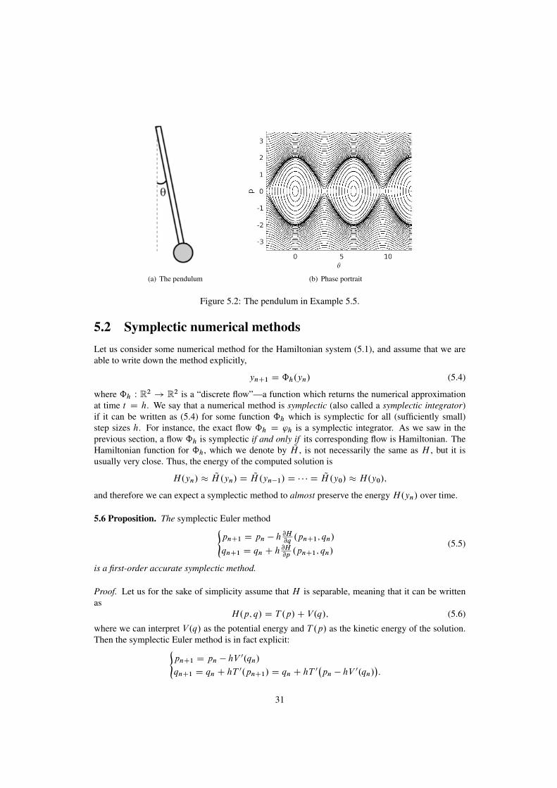
(a) The pendulum (b) Phase portrait

Figure 5.2: The pendulum in Example 5.5.

5.2 Symplectic numerical methodsLet us consider some numerical method for the Hamiltonian system (5.1), and assume that we areable to write down the method explicitly,

ynC1 D ˆh.yn/ (5.4)

where ˆh W R2 ! R2 is a “discrete flow”—a function which returns the numerical approximationat time t D h. We say that a numerical method is symplectic (also called a symplectic integrator)if it can be written as (5.4) for some function ˆh which is symplectic for all (sufficiently small)step sizes h. For instance, the exact flow ˆh D 'h is a symplectic integrator. As we saw in theprevious section, a flow ˆh is symplectic if and only if its corresponding flow is Hamiltonian. TheHamiltonian function for ˆh, which we denote by QH , is not necessarily the same as H , but it isusually very close. Thus, the energy of the computed solution is

H.yn/ � QH.yn/ D QH.yn�1/ D � � � D QH.y0/ � H.y0/;

and therefore we can expect a symplectic method to almost preserve the energy H.yn/ over time.

5.6 Proposition. The symplectic Euler method(pnC1 D pn � h

@H@q.pnC1; qn/

qnC1 D qn C h@H@p.pnC1; qn/

(5.5)

is a first-order accurate symplectic method.

Proof. Let us for the sake of simplicity assume that H is separable, meaning that it can be writtenas

H.p; q/ D T .p/C V.q/; (5.6)

where we can interpret V.q/ as the potential energy and T .p/ as the kinetic energy of the solution.Then the symplectic Euler method is in fact explicit:(

pnC1 D pn � hV0.qn/

qnC1 D qn C hT0.pnC1/ D qn C hT

0�pn � hV

0.qn/�:

31

Figure 5.3: The author is transported with the flow 't , but his area is preserved over time. The blackcurves are orbits of the flow.

Letting ˆh.pn; qn/ denote the right-hand side, we can compute

A WD rˆh.pn; qn/ D

1 �hV 00

hT 00 1 � h2T 00V 00

!where V 00 D V 00.qn/ and T 00 D T 00

�pn � hV

0.qn/�. It is now straightforward to check that A

satisfies (5.2), regardless of pn and qn.

5.7 Proposition. The Størmer–Verlet method18̂̂<̂:̂pnC1=2 D pn �

h2@H@q.pnC1=2; qn/

qnC1 D qn Ch2

�@H@p.pnC1=2; qn/C

@H@p.pnC1=2; qnC1/

�pnC1 D pnC1=2 �

h2@H@q.pnC1=2; qnC1/

(5.7)

is a second-order accurate symplectic method.1Named after Carl Størmer (1874–1957) and Loup Verlet (1931–), often (incorrectly) called the Störmer–Verlet method.

A professor in mathematics at the University of Oslo, Størmer did groundbreaking work in the modeling of aurora borealisusing differential equations. Størmer is also known for his photographs of people in Karl Johans gate, Oslo using a camerahidden under his jacket, in particular his photograph of Henrik Ibsen.

32

460 470 480 490 500

t

-1.5

-1

-0.5

0

0.5

1

1.5

p

Symplectic EulerExact solution

(a) Symplectic Euler

460 470 480 490 500

t

-1.5

-1

-0.5

0

0.5

1

1.5

p

Størmer-VerletExact solution

(b) Størmer–Verlet

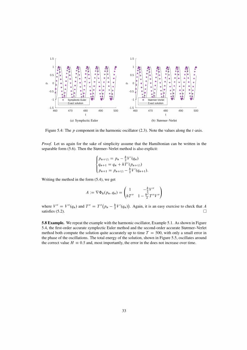
Figure 5.4: The p component in the harmonic oscillator (2.3). Note the values along the t -axis.

Proof. Let us again for the sake of simplicity assume that the Hamiltonian can be written in theseparable form (5.6). Then the Størmer–Verlet method is also explicit:8̂<̂

:pnC1=2 D pn �

h2V 0.qn/

qnC1 D qn C hT0.pnC1=2/

pnC1 D pnC1=2 �h2V 0.qnC1/:

Writing the method in the form (5.4), we get

A WD rˆh.pn; qn/ D

1 �

h2V 00

hT 00 1 � h2

2T 00V 00

!where V 00 D V 00.qn/ and T 00 D T 00

�pn �

h2V 0.qn/

�. Again, it is an easy exercise to check that A

satisfies (5.2).

5.8 Example. We repeat the example with the harmonic oscillator, Example 5.1. As shown in Figure5.4, the first-order accurate symplectic Euler method and the second-order accurate Størmer–Verletmethod both compute the solution quite accurately up to time T D 500, with only a small error inthe phase of the oscillations. The total energy of the solution, shown in Figure 5.5, oscillates aroundthe correct value H � 0:5 and, most importantly, the error in the does not increase over time.

33

460 470 480 490 500

t

0

0.1

0.2

0.3

0.4

0.5

0.6

H(p

,q)

Symplectic EulerExact solution

(a) Symplectic Euler

460 470 480 490 500

t

0

0.1

0.2

0.3

0.4

0.5

0.6

H(p

,q)

Størmer-VerletExact solution

(b) Størmer–Verlet

Figure 5.5: The total energy H.p; q/ for the harmonic oscillator (2.3). Note the values along thet -axis.

34

Bibliography

[1] J. C. Butcher. Numerical Methods for Ordinary Differential Equations. John Wiley & Sons, 3rdedition, 2016.

[2] E. Hairer and G. Wanner. Solving Ordinary Differential Equations II. Springer-Verlag BerlinHeidelberg, 2nd edition, 1996.

[3] A. Iserles. A First Course in the Numerical Analysis of Differential Equations. Cambridge Textsin Applied Mathematics. Cambridge University Press, 2nd edition, 2008.

35