Embed Size (px)
Citation preview
IMPLEMENTATION OF A CUTTING PLANE
METHOD FOR SEMIDEFINITE PROGRAMMING
by
Joseph G. Young
Submitted in Partial Fulfillment
of the Requirements for the Degree of
Masters of Science in Mathematics with Emphasis in Operations Research
and Statistics
New Mexico Institute of Mining and Technology
Socorro, New Mexico
May, 2004
ABSTRACT
Semidefinite programming refers to a class of problems that optimizes
a linear cost function while insuring that a linear combination of symmetric
matrices is positive definite. Currently, interior point methods for linear pro-
gramming have been extended to semidefinite programming, but they possess
some drawbacks. So, researchers have been investigating alternatives to inte-
rior point schemes. Krishnan and Mitchell[24, 19] investigated a cutting plane
algorithm that relaxes the problem into a linear program. Then, cuts are added
until the solution approaches optimality.
A software package was developed that reads and solves a semidefi-
nite program using the cutting plane algorithm. Properties of the algorithm
are analyzed and compared to existing methods. Finally, performance of the
algorithm is compared to an existing primal-dual code.
TABLE OF CONTENTS
LIST OF TABLES iii
LIST OF FIGURES iv
1. LINEAR PROGRAMMING 1
1.1 Introduction . . . . . . . . . . . . . . . . . . . . . . . . . . . . . 1
1.2 The Primal Problem . . . . . . . . . . . . . . . . . . . . . . . . 1
1.3 The Dual Problem . . . . . . . . . . . . . . . . . . . . . . . . . 2
2. SEMIDEFINITE PROGRAMMING 4
2.1 Introduction . . . . . . . . . . . . . . . . . . . . . . . . . . . . . 4
2.2 The Primal Problem . . . . . . . . . . . . . . . . . . . . . . . . 4
2.3 The Dual Problem . . . . . . . . . . . . . . . . . . . . . . . . . 5
2.4 A Primal-Dual Interior Point Method . . . . . . . . . . . . . . . 7
3. CUTTING PLANE ALGORITHM 13
3.1 Introduction . . . . . . . . . . . . . . . . . . . . . . . . . . . . . 13
3.2 Semiinfinite Program Reformulation of the Semidefinite Program 13
3.3 Linear Program Relaxation of the Semiinfinite Program . . . . . 14
3.4 Bounding the LP . . . . . . . . . . . . . . . . . . . . . . . . . . 18
3.5 Optimal Set of Constraints . . . . . . . . . . . . . . . . . . . . . 18
3.6 Removing Unneeded Constraints . . . . . . . . . . . . . . . . . 21
3.7 Resolving the Linear Program . . . . . . . . . . . . . . . . . . . 22
i
3.8 Stopping Conditions . . . . . . . . . . . . . . . . . . . . . . . . 23
3.9 Summary . . . . . . . . . . . . . . . . . . . . . . . . . . . . . . 24
3.10 Example . . . . . . . . . . . . . . . . . . . . . . . . . . . . . . . 25
4. COMPUTATIONAL RESULTS 31
4.1 Introduction . . . . . . . . . . . . . . . . . . . . . . . . . . . . . 31
4.2 Efficiency of the Algorithm . . . . . . . . . . . . . . . . . . . . . 31
4.2.1 Resolving the LP . . . . . . . . . . . . . . . . . . . . . . 31
4.2.2 Finding the Eigenvalues and Eigenvectors of Z . . . . . . 32
4.2.3 Constructing New Constraints . . . . . . . . . . . . . . . 32
4.3 Benchmarks . . . . . . . . . . . . . . . . . . . . . . . . . . . . . 33
4.4 Discussion of Results . . . . . . . . . . . . . . . . . . . . . . . . 33
5. CONCLUSIONS 38
5.1 Introduction . . . . . . . . . . . . . . . . . . . . . . . . . . . . . 38
5.2 Unique Properties . . . . . . . . . . . . . . . . . . . . . . . . . . 38
5.3 Performance . . . . . . . . . . . . . . . . . . . . . . . . . . . . . 39
5.4 Final Conclusions . . . . . . . . . . . . . . . . . . . . . . . . . . 40
REFERENCES 41
GLOSSARY 44
ii
LIST OF TABLES
4.1 Benchmark Results for Solver . . . . . . . . . . . . . . . . . . . 34
4.2 Benchmark Results for Solver . . . . . . . . . . . . . . . . . . . 35
4.3 Benchmark Results for Solver . . . . . . . . . . . . . . . . . . . 36
iii

LIST OF FIGURES
2.1 Summary of Predictor-Corrector Primal-Dual Method . . . . . . 9
3.1 Initial Constraints of LP . . . . . . . . . . . . . . . . . . . . . . 26
3.2 Constraints After One Iteration . . . . . . . . . . . . . . . . . . 27
3.3 Constraints After Two Iterations . . . . . . . . . . . . . . . . . 29
3.4 Constraints After Three Iterations . . . . . . . . . . . . . . . . . 30
iv

This report is accepted on behalf of the faculty of the Institute by the following
committee:
Brian Borchers, Advisor
Joseph G. Young Date
CHAPTER 1
LINEAR PROGRAMMING
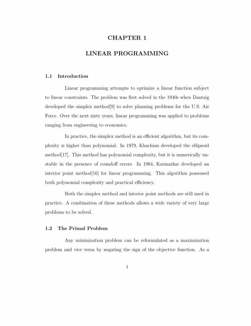
1.1 Introduction
Linear programming attempts to optimize a linear function subject
to linear constraints. The problem was first solved in the 1940s when Dantzig
developed the simplex method[9] to solve planning problems for the U.S. Air
Force. Over the next sixty years, linear programming was applied to problems
ranging from engineering to economics.
In practice, the simplex method is an efficient algorithm, but its com-
plexity is higher than polynomial. In 1979, Khachian developed the ellipsoid
method[17]. This method has polynomial complexity, but it is numerically un-
stable in the presence of roundoff errors. In 1984, Karmarkar developed an
interior point method[16] for linear programming. This algorithm possessed
both polynomial complexity and practical efficiency.
Both the simplex method and interior point methods are still used in
practice. A combination of these methods allows a wide variety of very large
problems to be solved.
1.2 The Primal Problem
Any minimization problem can be reformulated as a maximization
problem and vice versa by negating the sign of the objective function. As a
1

2
result, linear programming problems can be developed from either viewpoint.
However, a specific convention is developed and analyzed below for convenience.
The linear programming primal problem is given by
max cT x
subj Ax = b
xi ≥ 0 i = 1, 2, · · · , n
where c ∈ �m×1, A ∈ �m×n is nonsingular, and b ∈ �m×1 are given and
x ∈ �n×1 is variable[8]. We assume that the constraint matrix A has linearly
independent rows to simplify calculations.
The function x �→ cT x is referred as the objective function which
attains its optimal value at some optimal solution. In addition, any point
that satisfies the constraints is called feasible. Although all the constraints are
linear, each is labeled as either a linear constraint or a nonnegativity constraint.
The nonnegativity constraints prevent each element of the solution from being
negative. In a feasible solution, if xi = 0 for some i, then the constraint xi ≥ 0
is active. Otherwise, it is inactive.
1.3 The Dual Problem
Every linear programming maximization problem has an equivalent
minimization problem, or dual. These two problems provide useful information
about each other. For example, the value of the dual objective function provides
an upper bound for the value of primal objective function. This and other
results are discussed below.
3
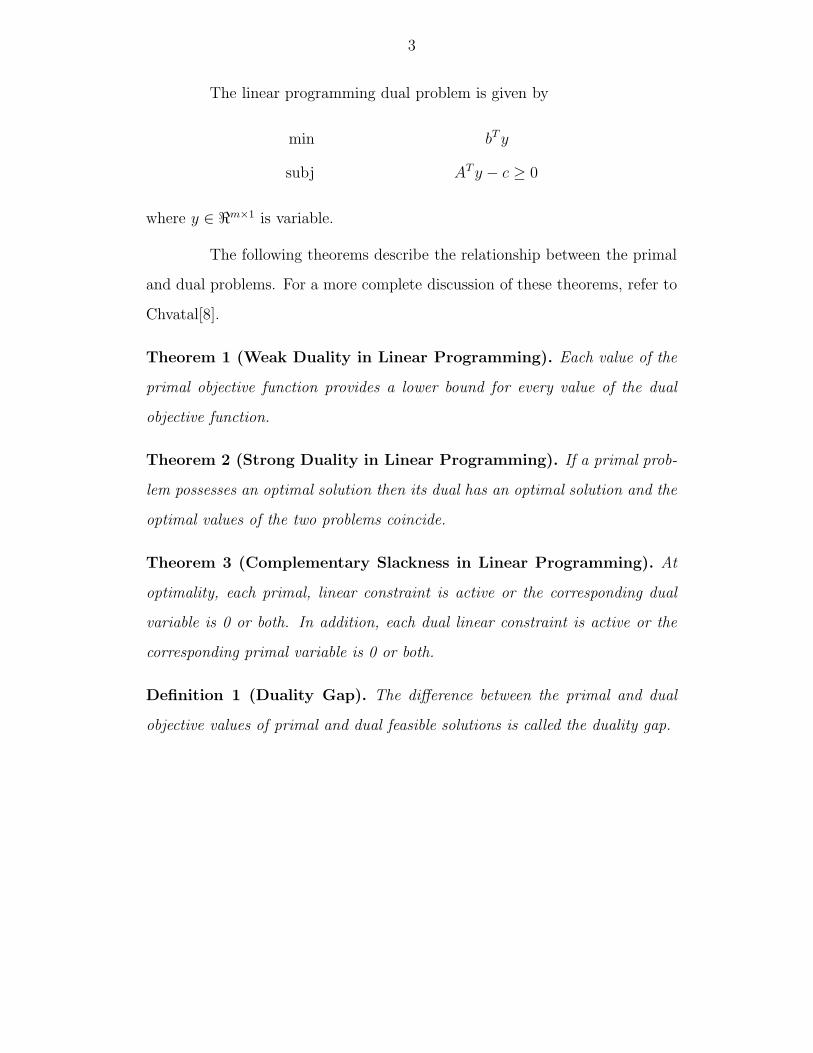
The linear programming dual problem is given by
min bT y
subj AT y − c ≥ 0
where y ∈ �m×1 is variable.
The following theorems describe the relationship between the primal
and dual problems. For a more complete discussion of these theorems, refer to
Chvatal[8].
Theorem 1 (Weak Duality in Linear Programming). Each value of the
primal objective function provides a lower bound for every value of the dual
objective function.
Theorem 2 (Strong Duality in Linear Programming). If a primal prob-
lem possesses an optimal solution then its dual has an optimal solution and the
optimal values of the two problems coincide.
Theorem 3 (Complementary Slackness in Linear Programming). At
optimality, each primal, linear constraint is active or the corresponding dual
variable is 0 or both. In addition, each dual linear constraint is active or the
corresponding primal variable is 0 or both.
Definition 1 (Duality Gap). The difference between the primal and dual
objective values of primal and dual feasible solutions is called the duality gap.
CHAPTER 2
SEMIDEFINITE PROGRAMMING
2.1 Introduction
Semidefinite programming is a generalization of linear programming
where the nonnegativity constraints are replaced with a single semidefinite
constraint. Although semidefinite programs were investigated as early as the
1960s[2], they were not thoroughly analyzed until the 1990s. Since then, many
effective algorithms have been developed such as the primal-dual interior point
method[15] and dual interior point method. These have been implemented
in several different codes such as CSDP[5], SDPA[12], DSDP[4], SDPT3[25],
and PENNON[18]. Further, semidefinite programming has been applied to
problems in areas ranging from electrical engineering[7] to graph theory[14].
Most modern algorithms solve semidefinite programs by generalizing
interior point methods for linear programming. These methods produce very
accurate results, but are computationally expensive for problems with more
than a few thousand variables. Currently, many researchers are attempting to
solve these large problems by parallelizing existing codes[3, 13].
2.2 The Primal Problem
Similar to linear programs, it unimportant for the primal to be a
minimization or a maximization problem. However, a specific convention is
4
5
developed for convenience. In the following section, Sn×n ⊂ �n×n is the set
of all symmetric n by n matrices. A matrix X ∈ Sn×n � 0 if it is positive
semidefinite.
The semidefinite programming primal problem is given by
max tr(CX)
subj A(X) = b (SDP)
X � 0
where C ∈ Sn×n, Ai ∈ Sn×n, A(x) =[tr(A1X), tr(A2X), . . . , tr(AmX)
]T, and
b ∈ �m×1 are given and the matrix X ∈ Sn×n is variable.
This problem is more general than the linear program formulated in
Chapter 1. Notice, the non-negativity has been replaced by a new semidefi-
niteness constraint. Note that, when X is diagonal, the semidefinite program
reduces to a linear program.
2.3 The Dual Problem
As in linear programming, every semidefinite programming primal
has a dual. The relationship between the primal and dual problems in semidef-
inite programs differs from linear programming in several ways. For example,
the primal and dual optimal values are not necessarily equal in semidefinite
programming. These and other results are discussed below.

6
The semidefinite dual problem is given by
min bT y
subj AT (y) − C = Z (SDD)
Z � 0
where AT (y) =m∑
i=1
yiAi, Ai ∈ Sn×n, and Z ∈ Sn×n � 0 are given and y ∈ �m×1
is variable.
Recall, the constraint matrix in a linear program is assumed to have
linearly independent rows. A similar assumption is made in semidefinite pro-
gramming. This simplifies many calculations.
Assumption 1. The constraint matrices are all linearly independent.
The following theorems describe the relationship between the primal
and dual problems. For a more complete discussion of these theorems, refer to
either de Klerk[10] or Wolkowicz et. al.[27].
Theorem 4 (Weak Duality in Semidefinite Programming). Each value
of the primal objective function provides a lower bound for every value of the
dual objective function.
Theorem 5 (Strong Duality in Semidefinite Programming). If the op-
timal primal and dual objective values are finite and both the primal and dual
problems contain strictly feasible solutions, then the optimal primal and dual
objective values are equal.
The strong duality theorem leads to the assumption.
7
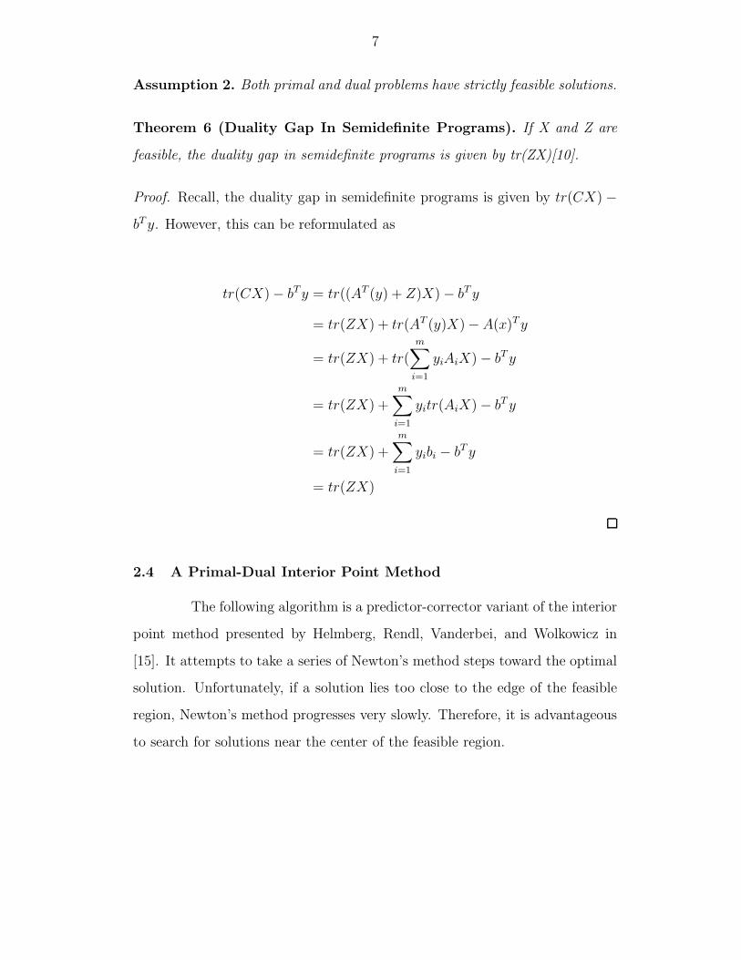
Assumption 2. Both primal and dual problems have strictly feasible solutions.
Theorem 6 (Duality Gap In Semidefinite Programs). If X and Z are
feasible, the duality gap in semidefinite programs is given by tr(ZX)[10].
Proof. Recall, the duality gap in semidefinite programs is given by tr(CX) −
bT y. However, this can be reformulated as
tr(CX) − bT y = tr((AT (y) + Z)X) − bT y
= tr(ZX) + tr(AT (y)X) − A(x)T y
= tr(ZX) + tr(
m∑i=1
yiAiX) − bT y
= tr(ZX) +m∑
i=1
yitr(AiX) − bT y
= tr(ZX) +
m∑i=1
yibi − bT y
= tr(ZX)
2.4 A Primal-Dual Interior Point Method
The following algorithm is a predictor-corrector variant of the interior
point method presented by Helmberg, Rendl, Vanderbei, and Wolkowicz in
[15]. It attempts to take a series of Newton’s method steps toward the optimal
solution. Unfortunately, if a solution lies too close to the edge of the feasible
region, Newton’s method progresses very slowly. Therefore, it is advantageous
to search for solutions near the center of the feasible region.

8
The development of the algorithm begins by introducing the dual
barrier problem
min bT y − μ(log det Z)
subj AT (y) − C = Z � 0 (DBP)
where μ > 0 ∈ � is the barrier parameter. When μ > 0, this objective function
penalizes movement toward the edge of the feasible region. Hence, Newton’s
method tends to find solutions toward the center of the feasible region. Un-
fortunately, determining an appropriate value of μ is difficult. So, the method
will make an initial predictor step to find an appropriate value of μ, then use
this barrier parameter in the corrector step.
The first order necessary conditions for optimality[23] are
Fd = Z + C − AT (y) = 0
Fp = b − A(X) = 0
XZ − μI = 0
where Fp and Fd are the primal and dual infeasibility respectively and final
equation is the complementarity condition.
The barrier function has two advantages. First, the derivative of
log det Z is Z−1. Second, log det Z is strictly concave. So, either there exists
a unique solution (Xμ, yμ, Zμ) to the first order necessary conditions or the
problem is unbounded.
The one parameter family (Xμ, yμ, Zμ), 0 ≤ μ ≤ ∞ is called the cen-
tral path. Given a point on the central path, it is possible to find its corre-

9
sponding value of μ by setting
μ =tr(ZX)
n
where the size of X and Z are both n by n. This follows immediately from
the complementary condition. It can be shown that, as μ approaches 0, the
optimal solution of the dual-barrier problem approaches the optimal solution
of the original problem[10].
The algorithm consists of two major steps. In the first, a Newton’s
method step is taken with μ = 0. In the second, this point is used to predict a
good value of μ for the corrector step. These steps are demonstrated in Figure
2.1.
Corrector StepStep
Central Path
Current Solution
Predictor
Figure 2.1: Summary of Predictor-Corrector Primal-Dual Method
The predictor step begins by taking a Newton’s method step for these
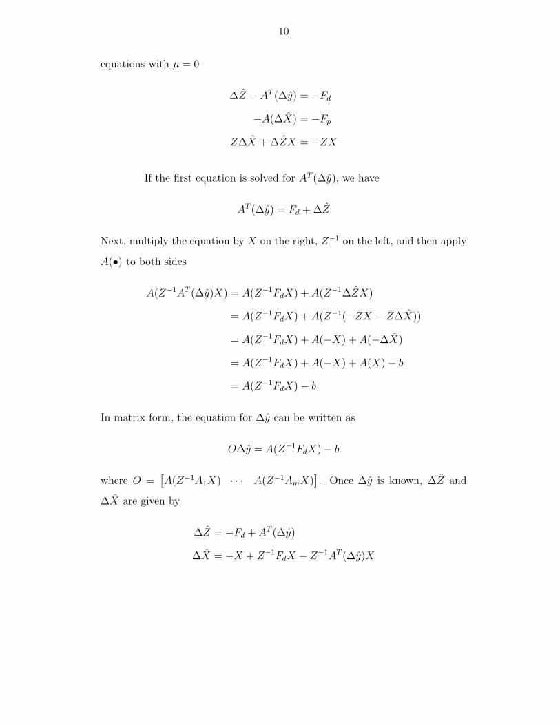
10
equations with μ = 0
ΔZ − AT (Δy) = −Fd
−A(ΔX) = −Fp
ZΔX + ΔZX = −ZX
If the first equation is solved for AT (Δy), we have
AT (Δy) = Fd + ΔZ
Next, multiply the equation by X on the right, Z−1 on the left, and then apply
A(•) to both sides
A(Z−1AT (Δy)X) = A(Z−1FdX) + A(Z−1ΔZX)
= A(Z−1FdX) + A(Z−1(−ZX − ZΔX))
= A(Z−1FdX) + A(−X) + A(−ΔX)
= A(Z−1FdX) + A(−X) + A(X) − b
= A(Z−1FdX) − b
In matrix form, the equation for Δy can be written as
OΔy = A(Z−1FdX) − b
where O =[A(Z−1A1X) · · · A(Z−1AmX)
]. Once Δy is known, ΔZ and
ΔX are given by
ΔZ = −Fd + AT (Δy)
ΔX = −X + Z−1FdX − Z−1AT (Δy)X

11
Note that if ΔX is not symmetric then we use the symmetric part of ΔX given
by
ΔXS =ΔX + ΔXT
2
The point (X + ΔX, y + Δy, Z + ΔZ) may not be feasible. So, a line search
must be used to find αD and αP such that (X + αP ΔX, y + αDΔy, Z + αDΔZ)
is feasible. Then, μ can be estimated by
μ =tr((Z + αDΔZ)(X + αP ΔX)
)n
The corrector step begins by computing a Newton’s method step using
the value of μ estimated in the predictor step
ΔZ − AT (Δy) = −Fd
−A(ΔX) = −Fp
ZΔX + ΔZX = −ZX + μI
The equations are solved similarly to those in the predictor step. However,
since we reintroduced the barrier parameter, the change in y is given by
OΔy = A(Z−1FdX) − b + A(μZ−1)
Once y is known, the same equations are used to determine both Z and X
ΔZ = −Fd + AT (Δy)
ΔX = −X + Z−1FdX − Z−1AT (Δy)X
As before, if these matrices are not symmetric, their symmetric parts are taken
instead. Finally, since the point (X+ΔX, y+Δy, Z+ΔZ) may not be feasible,

12
a line search must be used to find αD and αP such that (X + αP ΔX, y +
αDΔy, Z + αDΔZ) is feasible.
This algorithm iterates until both the primal and dual solutions are
feasible and the resulting duality gap becomes sufficiently small.
CHAPTER 3
CUTTING PLANE ALGORITHM
3.1 Introduction
Krishnan and Mitchell[24, 19] developed the cutting plane method
by reformulating the semidefinite program into a semiinfinite program. Then,
they relaxed the semiinfinite program into a linear program. Since the optimal
solution to the relaxed linear program is not necessarily feasible in the semidef-
inite program, linear cuts are iteratively added until the solution approaches
feasibility and optimality.
3.2 Semiinfinite Program Reformulation of the Semidefinite Pro-gram
An alternative definition of positive semidefinite leads to a reformu-
lation of the semidefinite program into a semiinfinite program.
Theorem 7. A matrix Z is positive semidefinite if and only if dT Zd ≥ 0 ∀d ∈
B ⊂ �n×n where B is a ball about the origin.
Proof. Recall that Z is positive semidefinite if and only if its inner product
with all rank one matrices is greater than or equal to zero. So, take any d ∈ �n
and let d = d‖d‖
r where r is the radius of the ball about the origin. As a result,
13
14
d is simply a scaled version of d that lies within the ball. If we take dTZd then
dT Zd =
(dT
‖d‖r
)Z
(d
‖d‖r
)
=
(r
‖d‖
)2
dTZd
Thus, dT Zd ≥ 0 if and only if dT Zd ≥ 0. Consequently, we only need to
consider vectors in B when determining whether Z is positive definite.
The semiinfinite dual problem is given by
min bT y
subj dT (AT (y) − C)d ≥ 0 ∀d ∈ B (SID)
where B is a ball about the origin. Note that the problem must be relaxed
before a solution can be found.
3.3 Linear Program Relaxation of the Semiinfinite Program
As discussed above, very sophisticated solvers exist for linear pro-
grams. So, relaxing the semiinfinite program into a linear program will allow
a near feasible solution to be found very quickly.
The linear programming relaxation is found by taking a finite subset of
the infinite number of constraints from the semiinfinite program. The resulting
dual problem is given by
min bT y
subj dTj (AT (y) − C)dj ≥ 0 j = 1, . . . , p (LPD)
where p is arbitrary, but finite.
15
The primal problem is obtained by finding the dual of the dual linear
program. The dual linear program can be rewritten as
min bT y
subj dTj (
m∑i=1
yiAi − C)dj ≥ 0 j = 1, . . . , p
Then, the constraint can be reformulated as
dTj (
m∑i=1
yiAi − C)dj ≥ 0 ⇐⇒ dTj (
m∑i=1
yiAi)dj ≥ dTj Cdj
⇐⇒m∑
i=1
yidTj Aidj ≥ dT
j Cdj
⇐⇒
m∑i=1
yitr(djdTj Ai) ≥ dT
j Cdj
This allows the primal problem to be formulated as
max
p∑j=1
tr(CdjdTj )xj
subj
p∑j=1
tr(djdTj Ai)xj = bi i = 1, . . . , m
xj ≥ 0
Again, the constraint can be reformulatedp∑
j=1
tr(djdTj Ai)xj = bi ⇐⇒
p∑j=1
tr(djdTj Ai)xj = bi
⇐⇒
p∑j=1
tr(Ai(djdTj xj)) = bi
⇐⇒ tr(Ai(
p∑j=1
djdTj xj)) = bi
⇐⇒ A
(p∑
j=1
xjdjdTj
)= b

16
Finally, the primal problem is given by
max tr
(C(
p∑j=1
xjdjdTj )
)
subj A
(p∑
j=1
xjdjdTj
)= b (LPP)
where x ∈ �++, all non-negative reals.
Since the dual LP is a relaxation of the dual SDP, a feasible solution
of the dual LP isn’t necessarily feasible in the dual SDP. Further, there is
no guarantee that the dual LP is bounded. So, it is possible to construct
a relaxation where the primal LP is infeasible. However, if the dual LP is
bounded, the primal LP is more constrained than the primal SDP. So, all
feasible solutions of the primal LP are feasible in the primal SDP. This is given
formally by the following theorem.
Theorem 8 (Linear Primal Feasibility Implies Semidefinite Feasibil-
ity). Any feasible solution to the linear relaxation of the SDP primal is also
feasible in the SDP primal.
Proof. Let, X =p∑
j=1
xjdjdTj
We must show that A(X) = b and X � 0.
The first part following immediately since A
(p∑
j=1
xjdjdTj
)= b.
17
The second part can seen by noting
dT Xd = dT
(p∑
j=1
xjdjdTj
)d
=
p∑j=1
xjdT (djd
Tj )d
=
p∑j=1
xj(dT dj)
2
≥ 0
since xj ≥ 0 for all j.
Typically, the duality gap provides a measure of how far a method is
from converging. However, in this method, the duality gap of the semidefinite
program is zero for all optimal solutions to the linear relaxation.
Theorem 9 (Optimallity of the Linear Relaxation Implies Zero Semidef-
inite Duality Gap). The duality gap of the semidefinite program is zero for
all optimal solutions to the linear programming relaxation.
Proof. The duality gap of a linear program is zero at optimality. By con-
struction, the objective value of the semidefinite program is the same as the
relaxation. So, when the relaxation is at optimality, the duality gap for both
programs is zero.
For a solution (X∗, y∗, Z∗) to be optimal, it must satisfy three crite-
ria: primal feasibility, dual feasibility, and a zero duality gap. The following
theorem shows that if Z∗ � 0 then the solution is optimal.
18
Theorem 10 (Feasibility with Respect to the Dual Semidefinite Con-
straint Implies Optimallity). Let y∗ be an optimal solution to the linear
dual and X∗ =p∑
j=1
xjdjdTj . If Z∗ = AT (y∗) − C � 0, the solution (X∗, y∗, Z∗)
is optimal.
Proof. We must show that all three criteria for optimality are met.
First, Theorem 8 shows the primal solution is feasible. Second, the
dual solution is feasible since we assumed that Z∗ � 0 and we defined Z∗ =
AT (y∗)−C. Finally, Theorem 9 demonstrates that the duality gap is zero.
3.4 Bounding the LP
There exists a constraint that bounds the objective function of the
form bT y ≥ α. If the original semidefinite program is bounded, then α can be
chosen such that every feasible solution satisfies the above constraint. Although
this constraint insures the LP is bounded, the choice of α is problem dependent.
It is important to note that the constraint bT y ≥ α does not follow the
form dT (AT (y) − C)d ≥ 0. So, it is not possible to generate a primal solution
X until this constraint has been removed from the relaxation. Techniques for
removing constraints are discussed later.
3.5 Optimal Set of Constraints
Assume that the current optimal solution of the dual LP is infeasible
in the SDP dual. Then, adding more constraints to the problem should produce
a solution closer to feasibility. These new constraints are called a deep cuts since
the current feasible solution is excluded from the new feasible set. However,
19
not all cuts will produce an equivalent improvement. Some constraints are
redundant and others produce a very marginal gain. So, an intelligent choice
of constraints allows the method to converge faster.
Theorem 11 (Non-Negativity of Diagonal Elements). For every feasible
solution to the dual SDP, the dual LP must satisfy
m∑i=1
[Ai]jjyi ≥ Cjj
where 1 ≤ j ≤ n.
Proof. Let Z be positive semidefinite and let ej ∈ �n×n be an elementary vector
with a 1 in the jth position. Since Z � 0,
eTj Zej ≥ 0 ⇐⇒ [Z]jj ≥ 0
⇐⇒ [AT (y) − C]jj ≥ 0
⇐⇒
m∑i=1
[Ai]jjyi ≥ Cjj
These cuts are not required for the algorithm to function, but they
tend to enhance the performance of the method. Further, they follow the form
eTi (AT (y) − C)ei ≥ 0. So, it is possible to generate a primal solution X while
these constraints are part of the relaxation.
Theorem 12 (Deep Cut). The cut given by
d(k)T AT (y)d(k) ≥ d(k)T Cd(k)
where d(k) ∈ B � d(k)T (AT (y(k)) − C)d(k) < 0 and y(k) is the optimal solution
of LP dual at iteration k, excludes the current feasible solution.
20
Proof. A deep cut is a constraint that excludes the current feasible solution
from the new feasible set. So, we must show the current point is infeasi-
ble if the new constraint is added. However, this follows immediately since
d(k)T (AT (y(k)) − C)d(k) < 0.
The following theorem describes how to find d(k) quickly and effi-
ciently.
Theorem 13 (Deep Cuts Over a Unit Ball in 2-Norm). Let B = {d �
‖d‖2 ≤ 1}. Every eigenvector d(k) that corresponds to a negative eigenvalue of
AT (y(k)) − C describes a deep cut.
Proof. Let λ(k) be the eigenvalue of AT (y(k)) − C that corresponds to d(k).
Notice,
d(k)T(AT (y(k)) − C
)d(k) = d(k)T λ(k)d(k)
= λ(k)
However, λ(k) < 0 by assumption. So, the cut is deep.
Although any eigenvector corresponding to a negative eigenvalue de-
scribes a deep cut, generating all eigenvectors of a large matrix is expensive.
So, the following theorem describes which eigenvectors produce the deepest
possible cut
Theorem 14 (Optimal Deep Cut Over a Unit Ball in 2-Norm). Let
B = {d � ‖d‖22 ≤ 1}. The cut created from the eigenvector that corresponds
to the minimum eigenvalue of Z (k) maximizes the distance from the current
solution and the feasible region.

21
Proof. This problem is equivalent to
mind(k)
d(k)T Z(k)d(k) subj ‖d(k)‖22 ≤ 1
There are two cases two consider.
First, assume that the constraint is inactive. This implies that the
minimum is an unconstrained minimum. However, this minimum can’t exist
unless Z(k) is positive definite. But, this is a contradiction since by assumption
Z(k) �� 0.
Second, assume that the constraint is active. From the first order
necessary conditions, Z(k)d = λd. So, all eigenvectors of Z (k) are stationary
points. Let d(k) be an eigenvector with corresponding eigenvalue λ(k). Then,
d(k)T Z(k)d(k) = d(k)T λ(k)d(k) = λ(k). Thus, the cut created from the minimum
eigenvalue’s eigenvector maximizes the infeasibility of the current solution.
3.6 Removing Unneeded Constraints
The cutting plane method leads to a huge build up of constraints over
time. However, as the algorithm progresses, many of these constraints become
unneeded. Hence, at every iteration, all inactive and redundant constraints
should be removed.
Inactive constraints are easily determined and removed. However, re-
dundant constraints are more elusive. If the dual variable corresponding to
a constraint is zero, then the constraint does not contribute to the solution.
However, not all constraints with a corresponding zero dual variable can be re-
moved. Eliminating one constraint may change whether another is redundant.
22
A fast method to eliminate unneeded constraints simply looks at the
basis of the solved linear program. If a slack variable is in the basis, the
corresponding constraint is eliminated. Since it is possible that a constraint is
degenerate, this elimination method is not entirely safe. However, in practice,
useful constraints are rarely eliminated. Finally, in practice, it is advantageous
to preserve the constraints that maintain the non-negativity of the diagonal
elements of Z.
3.7 Resolving the Linear Program
It is very costly to resolve the linear program from scratch at every
iteration. Fortunately, the dual simplex method provides a fast restart option.
Let y be a solution to the dual linear program. Let y be a vector where each
element corresponds to an active constraint. Let A be the constraint matrix
with all inactive constraints removed. Then, y is feasible in A since
[AT y − c]k =m∑
i=1
Aikyi
=∑
i∈Active
Aikyi
=∑
Aikyi
≥ 0
If new constraints are added and their corresponding dual variables
set to 0, then the solution remains dual feasible. Hence, the dual simplex
method can be warm started using this new constraint matrix and solution.
Since the distance between solutions at each iteration changes only slightly,
this gives a large performance improvement.
23
3.8 Stopping Conditions
The seventh DIMACS implementation challenge defined six different
error measures
err1(X, y, Z) =‖A(X) − b‖F
1 + ‖b‖1
err2(X, y, Z) = max
{0,
−λmin(X)
1 + ‖b‖1
}
err3(X, y, Z) =‖AT (y) + Z − C‖F
1 + ‖C‖1
err4(X, y, Z) = max
{0,
−λmin(Z)
1 + ‖C‖1
}
err5(X, y, Z) =tr(CX) − bT y
1 + |tr(CX)| + |bT y|
err6(X, y, Z) =tr(ZX)
1 + |tr(CX)| + |bT y|
where λmin(X) is the minimum eigenvalue of X[22].
The first two errors describe the primal feasibility with respect to the
linear constraints and the semidefinite constraint. Since this method creates
a series of strictly primal feasible solutions, the first two error measures are
zero. The second two errors describe the dual feasibility with respect to the
linear constraints and the semidefinite constraint. Because this method creates
a series of dual solutions that are strictly feasible with respect to the linear
constraints, the third error measure is zero. Finally, the last two error measures
describe the duality gap. Since the method produces solutions where the duality
gap is zero, the fifth error measure is zero. Because Z is not typically feasible,
the sixth error measure is meaningless.
These error measures give a good indication of how close a solution is

24
to optimality. However, in this method, all of the error measures are zero save
the fourth. So, the feasibility of the dual with respect to the semidefinite con-
straint provides a stopping criteria. Unfortunately, the fourth DIMACS error
does not provide a very good stopping criteria. In general, the minimum eigen-
value of Z does not monotonically approach 0. Further, the objective function
may approach optimality long before Z approaches feasibility. In practice, it
is difficult to reduce the fourth error measure to less that .1. Despite this the
solver uses this error measure as its stopping criteria.
Ideally, we would like to have a set of feasible primal and dual so-
lutions. Then, we could base our stopping criteria off of the fifth and sixth
DIMACS error measures that describe the duality gap. So, it would help
to find a perturbation of Z such that we maintain feasibility, but the size
of the perturbation converges to zero as the solution converges to optimal-
ity. Let Z(k) = Z(k) + E(k) � 0. Since all feasible solutions have the form
Z = AT (y) − C, an appropriate perturbation E(k) would be found such that
E(k) = AT (e(k)) while its norm converges to 0 as the method converges toward
optimality. Once found, Z(k) would provide an upper bound to the problem
that converges toward optimality. Unfortunately, there is no general method
to determine E(k).
3.9 Summary
The cutting plane algorithm can be summarized as
Add diagonal element non-negativity constraints
Add bounding constraint
25
While the fourth DIMACS error measure > Tolerance
Remove inactive constraints
Add new constraints
Resolve LP
End While
3.10 Example
A simple two-dimensional semidefinite program is
min y1 + y2
subj
[2 44 0
]y1 +
[2 00 6
]y2 �
[1 22 3
]
We’ll assume that the minimum value our objective function could
attain is 0. So, our initial relaxation is
min y1 + y2
subj 2y1 + 2y2 ≥ 1
6y2 ≥ 3
y1 + y2 ≥ 0
Notice that the first two constraints insure the diagonal elements of Z will be
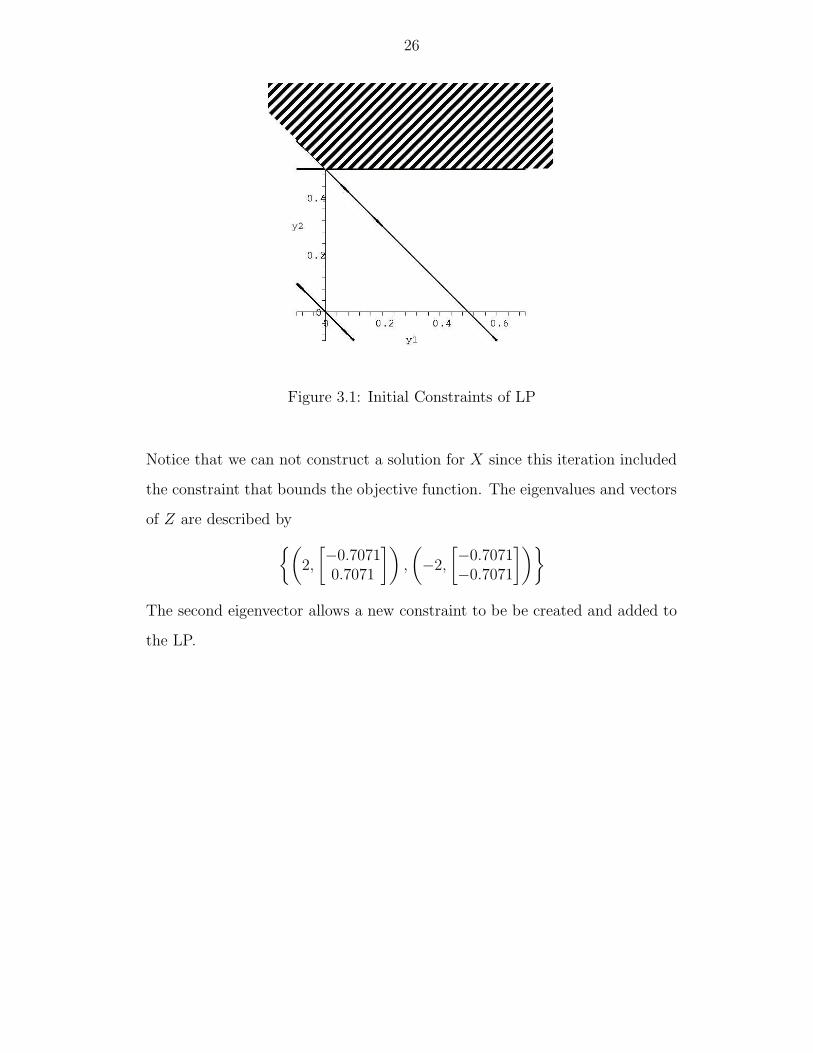
positive while the third constraint bounds the LP. The feasible region is shown
in Figure 3.1. After solving the LP, we find that the optimal solution is (0, .5)
and the optimal value of .5. Since the third constraint is no longer tight, it will
be removed from the constraint matrix. Our current SDP solution is given by
(X, y, Z) =
(NA,
[0.5
],
[0 −2−2 0
])
26
Figure 3.1: Initial Constraints of LP
Notice that we can not construct a solution for X since this iteration included
the constraint that bounds the objective function. The eigenvalues and vectors
of Z are described by{(2,
[−0.70710.7071
]),
(−2,
[−0.7071−0.7071
])}
The second eigenvector allows a new constraint to be be created and added to
the LP.
27
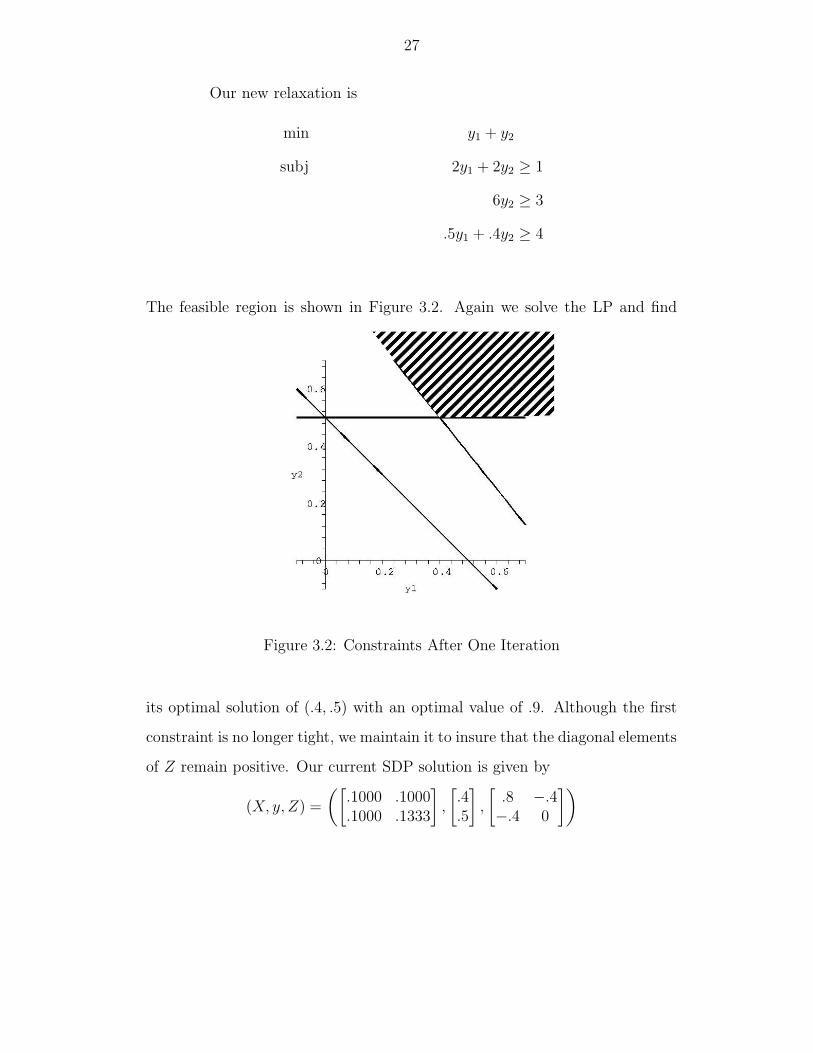
Our new relaxation is
min y1 + y2
subj 2y1 + 2y2 ≥ 1
6y2 ≥ 3
.5y1 + .4y2 ≥ 4
The feasible region is shown in Figure 3.2. Again we solve the LP and find
Figure 3.2: Constraints After One Iteration
its optimal solution of (.4, .5) with an optimal value of .9. Although the first
constraint is no longer tight, we maintain it to insure that the diagonal elements
of Z remain positive. Our current SDP solution is given by
(X, y, Z) =
([.1000 .1000.1000 .1333
],
[.4.5
],
[.8 −.4−.4 0
])
28
The eigenvalue and eigenvector pairs of Z are given by{(.96596,
[−.92388.38268
]),
(−.16569,
[−.38268−.92388
])}
We use the second eigenvector to construct a new constraint that is added to
the LP.
Our new relaxation is given by
min y1 + y2
subj 2y1 + 2y2 ≥ 1
6y2 ≥ 3
.5y1 + .4y2 ≥ 4
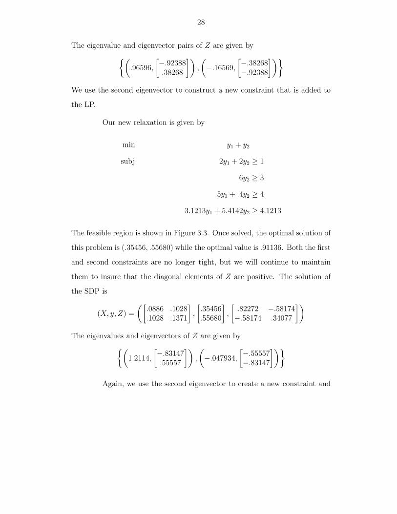
3.1213y1 + 5.4142y2 ≥ 4.1213
The feasible region is shown in Figure 3.3. Once solved, the optimal solution of
this problem is (.35456, .55680) while the optimal value is .91136. Both the first
and second constraints are no longer tight, but we will continue to maintain
them to insure that the diagonal elements of Z are positive. The solution of
the SDP is
(X, y, Z) =
([.0886 .1028.1028 .1371
],
[.35456.55680
],
[.82272 −.58174−.58174 .34077
])
The eigenvalues and eigenvectors of Z are given by{(1.2114,
[−.83147.55557
]),
(−.047934,
[−.55557−.83147
])}
Again, we use the second eigenvector to create a new constraint and
29
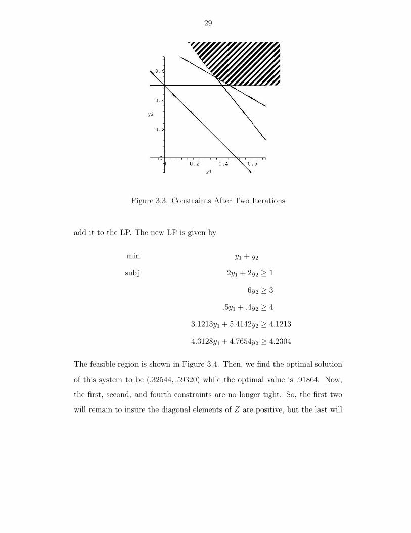
Figure 3.3: Constraints After Two Iterations
add it to the LP. The new LP is given by
min y1 + y2
subj 2y1 + 2y2 ≥ 1
6y2 ≥ 3
.5y1 + .4y2 ≥ 4
3.1213y1 + 5.4142y2 ≥ 4.1213
4.3128y1 + 4.7654y2 ≥ 4.2304
The feasible region is shown in Figure 3.4. Then, we find the optimal solution
of this system to be (.32544, .59320) while the optimal value is .91864. Now,
the first, second, and fourth constraints are no longer tight. So, the first two
will remain to insure the diagonal elements of Z are positive, but the last will
30
Figure 3.4: Constraints After Three Iterations
be removed. The solution to the SDP is given by
(X, y, Z) =
([.0814 .1047.1047 .1395
],
[.32544.59320)
],
[.82272 −.58174−.58174 .34077
])
The eigenvalue and eigenvector pairs of Z are given by{(1.4102,
[−.77307.63432
]),
(−.013706
[−.63432−.77307
])}
We’ll stop at this step since the normed eigenvalue error is approximately
.002284.
In summary, this process is repeated until the normed eigenvalue error
is sufficiently small.
CHAPTER 4
COMPUTATIONAL RESULTS
4.1 Introduction
Krishnan and Mitchell proved that this method possesses polynomial
time convergence[19]. However, this doesn’t necessarily mean the algorithm
performs well. In the following chapter, the method’s computational properties
will be discussed.
4.2 Efficiency of the Algorithm
The three parts of the algorithm that take the most computational
time are resolving the LP, finding the eigenvalues of Z, and constructing new
constraints.
4.2.1 Resolving the LP
In general, the constraint matrix is fully dense. Further, the matrix
contains m columns and p rows where p is the number of linear constraints
necessary to approximate a corner of the semidefinite region. In practice, p
is bounded, but it depends on the problem. The benchmark results tabulate
several of these bounds.
The discussion above describes how to construct a new dual feasible
solution after the LP has been modified. Once this dual feasible solution is
31
32
obtained, it can be used to warm start the dual simplex method. In practice,
this provides very good performance. However, there exist problems where
adding new cuts significantly changes the optimal solution such as the control
problems from SDPLIB[6]. In this case, each resolve becomes more expensive.
In all but the most pathological cases, this step is an order of magnitude faster
that constructing new constraints.
4.2.2 Finding the Eigenvalues and Eigenvectors of Z
The dual solution Z is block diagonal. So, the eigenvalues of Z are the
eigenvalues of each block. Since non-negativity of the diagonal elements of Z is
enforced, diagonal blocks can be ignored. The remaining blocks are typically
dense, so LAPACK[1] routines that operate on symmetric matrices may be
used to find the eigenvalues. Since only a few eigenvalues are needed, Lanczos
method could be used to find eigenvalues. However, since each block of Z is
typically dense and this step of the algorithm is two orders of magnitude faster
than constructing the constraints, any benefit from using the Lanczos method
would be negligible.
4.2.3 Constructing New Constraints
Once the eigenvalues and eigenvectors of Z are known, new constraints
are added. Each coefficient of every new constraint requires O(n2) operations.
So, generating all constraints requires a total of O(cmn2) operations where
c is the number of cuts. Typically, each Ai is relatively sparse. So, sparse
linear algebra routines can dramatically improve performance. Even with these
optimizations, this step is typically an order of magnitude more expensive than
33
the other two.
4.3 Benchmarks
The method was benchmarked using problems from SDPLIB. In each
test case, the following external libraries are referenced. First, COIN-OR[20]
using GLPK[21] solved the linear programming relaxations. Since the resulting
constraint matrices are typically dense, COIN-OR was compiled using dense
factorizations. Second, LAPACK’s[1] DSYEVR routine found the eigenvalues.
The DSYEVR routine uses the relatively robust representations (RRR)[11]
driver for calculating eigenvalues. Finally, ATLAS[26] BLAS computed the
rest of the linear algebra.
Each test problem used the exact same input parameters. First, we
compute 10 cuts per block of Z. Second, we assume the method has converged
when the fourth DIMACS error falls below .1. Third, we assume the minimum
possible objective value is -1000. Finally, we limit the solver to 15 minutes of
computation.
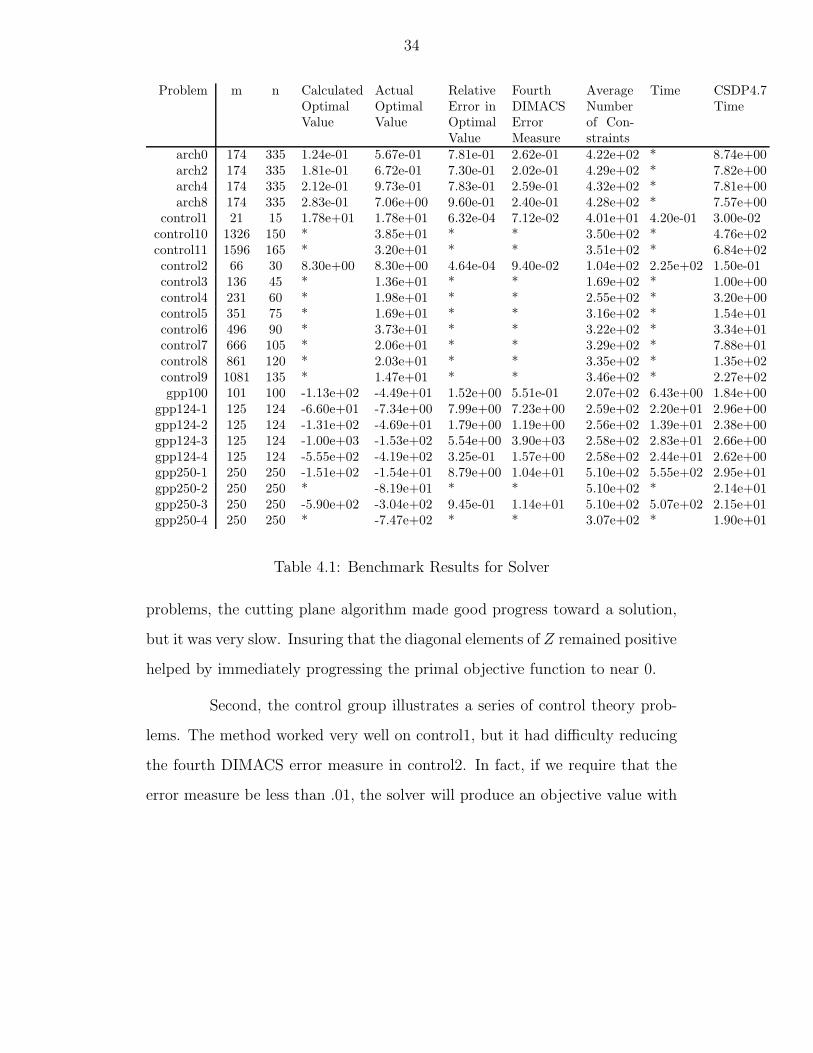
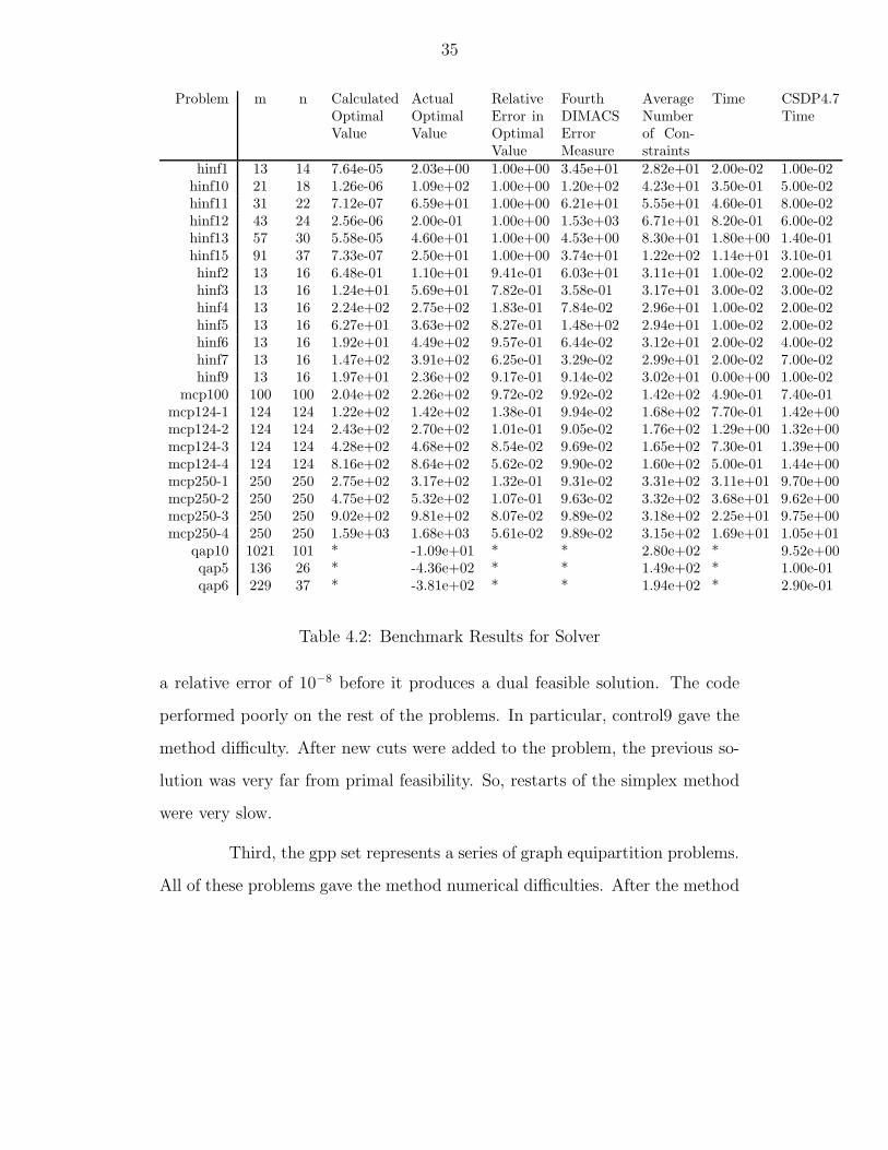
The results are summarized in Tables 4.1, 4.2, and 4.3. A star in the
time column means the method reached the time limit. A star in other columns
means the method did not progress from the lower bound.
4.4 Discussion of Results
Each set of problems possessed different runtime performance and
results. These are discussed below.
First, the arch set is a series of topology design problems. On these
34
Problem m n Calculated
OptimalValue
Actual
OptimalValue
Relative
Error inOptimal
Value
Fourth
DIMACSError
Measure
Average
Numberof Con-
straints
Time CSDP4.7
Time
arch0 174 335 1.24e-01 5.67e-01 7.81e-01 2.62e-01 4.22e+02 * 8.74e+00
arch2 174 335 1.81e-01 6.72e-01 7.30e-01 2.02e-01 4.29e+02 * 7.82e+00arch4 174 335 2.12e-01 9.73e-01 7.83e-01 2.59e-01 4.32e+02 * 7.81e+00
arch8 174 335 2.83e-01 7.06e+00 9.60e-01 2.40e-01 4.28e+02 * 7.57e+00control1 21 15 1.78e+01 1.78e+01 6.32e-04 7.12e-02 4.01e+01 4.20e-01 3.00e-02
control10 1326 150 * 3.85e+01 * * 3.50e+02 * 4.76e+02
control11 1596 165 * 3.20e+01 * * 3.51e+02 * 6.84e+02control2 66 30 8.30e+00 8.30e+00 4.64e-04 9.40e-02 1.04e+02 2.25e+02 1.50e-01
control3 136 45 * 1.36e+01 * * 1.69e+02 * 1.00e+00
control4 231 60 * 1.98e+01 * * 2.55e+02 * 3.20e+00control5 351 75 * 1.69e+01 * * 3.16e+02 * 1.54e+01
control6 496 90 * 3.73e+01 * * 3.22e+02 * 3.34e+01control7 666 105 * 2.06e+01 * * 3.29e+02 * 7.88e+01
control8 861 120 * 2.03e+01 * * 3.35e+02 * 1.35e+02
control9 1081 135 * 1.47e+01 * * 3.46e+02 * 2.27e+02gpp100 101 100 -1.13e+02 -4.49e+01 1.52e+00 5.51e-01 2.07e+02 6.43e+00 1.84e+00
gpp124-1 125 124 -6.60e+01 -7.34e+00 7.99e+00 7.23e+00 2.59e+02 2.20e+01 2.96e+00
gpp124-2 125 124 -1.31e+02 -4.69e+01 1.79e+00 1.19e+00 2.56e+02 1.39e+01 2.38e+00gpp124-3 125 124 -1.00e+03 -1.53e+02 5.54e+00 3.90e+03 2.58e+02 2.83e+01 2.66e+00
gpp124-4 125 124 -5.55e+02 -4.19e+02 3.25e-01 1.57e+00 2.58e+02 2.44e+01 2.62e+00gpp250-1 250 250 -1.51e+02 -1.54e+01 8.79e+00 1.04e+01 5.10e+02 5.55e+02 2.95e+01
gpp250-2 250 250 * -8.19e+01 * * 5.10e+02 * 2.14e+01
gpp250-3 250 250 -5.90e+02 -3.04e+02 9.45e-01 1.14e+01 5.10e+02 5.07e+02 2.15e+01gpp250-4 250 250 * -7.47e+02 * * 3.07e+02 * 1.90e+01
Table 4.1: Benchmark Results for Solver
problems, the cutting plane algorithm made good progress toward a solution,
but it was very slow. Insuring that the diagonal elements of Z remained positive
helped by immediately progressing the primal objective function to near 0.
Second, the control group illustrates a series of control theory prob-
lems. The method worked very well on control1, but it had difficulty reducing
the fourth DIMACS error measure in control2. In fact, if we require that the
error measure be less than .01, the solver will produce an objective value with
35
Problem m n Calculated
OptimalValue
Actual
OptimalValue
Relative
Error inOptimal
Value
Fourth
DIMACSError
Measure
Average
Numberof Con-
straints
Time CSDP4.7
Time
hinf1 13 14 7.64e-05 2.03e+00 1.00e+00 3.45e+01 2.82e+01 2.00e-02 1.00e-02
hinf10 21 18 1.26e-06 1.09e+02 1.00e+00 1.20e+02 4.23e+01 3.50e-01 5.00e-02hinf11 31 22 7.12e-07 6.59e+01 1.00e+00 6.21e+01 5.55e+01 4.60e-01 8.00e-02
hinf12 43 24 2.56e-06 2.00e-01 1.00e+00 1.53e+03 6.71e+01 8.20e-01 6.00e-02hinf13 57 30 5.58e-05 4.60e+01 1.00e+00 4.53e+00 8.30e+01 1.80e+00 1.40e-01
hinf15 91 37 7.33e-07 2.50e+01 1.00e+00 3.74e+01 1.22e+02 1.14e+01 3.10e-01
hinf2 13 16 6.48e-01 1.10e+01 9.41e-01 6.03e+01 3.11e+01 1.00e-02 2.00e-02hinf3 13 16 1.24e+01 5.69e+01 7.82e-01 3.58e-01 3.17e+01 3.00e-02 3.00e-02
hinf4 13 16 2.24e+02 2.75e+02 1.83e-01 7.84e-02 2.96e+01 1.00e-02 2.00e-02
hinf5 13 16 6.27e+01 3.63e+02 8.27e-01 1.48e+02 2.94e+01 1.00e-02 2.00e-02hinf6 13 16 1.92e+01 4.49e+02 9.57e-01 6.44e-02 3.12e+01 2.00e-02 4.00e-02
hinf7 13 16 1.47e+02 3.91e+02 6.25e-01 3.29e-02 2.99e+01 2.00e-02 7.00e-02hinf9 13 16 1.97e+01 2.36e+02 9.17e-01 9.14e-02 3.02e+01 0.00e+00 1.00e-02
mcp100 100 100 2.04e+02 2.26e+02 9.72e-02 9.92e-02 1.42e+02 4.90e-01 7.40e-01
mcp124-1 124 124 1.22e+02 1.42e+02 1.38e-01 9.94e-02 1.68e+02 7.70e-01 1.42e+00mcp124-2 124 124 2.43e+02 2.70e+02 1.01e-01 9.05e-02 1.76e+02 1.29e+00 1.32e+00
mcp124-3 124 124 4.28e+02 4.68e+02 8.54e-02 9.69e-02 1.65e+02 7.30e-01 1.39e+00
mcp124-4 124 124 8.16e+02 8.64e+02 5.62e-02 9.90e-02 1.60e+02 5.00e-01 1.44e+00mcp250-1 250 250 2.75e+02 3.17e+02 1.32e-01 9.31e-02 3.31e+02 3.11e+01 9.70e+00
mcp250-2 250 250 4.75e+02 5.32e+02 1.07e-01 9.63e-02 3.32e+02 3.68e+01 9.62e+00mcp250-3 250 250 9.02e+02 9.81e+02 8.07e-02 9.89e-02 3.18e+02 2.25e+01 9.75e+00
mcp250-4 250 250 1.59e+03 1.68e+03 5.61e-02 9.89e-02 3.15e+02 1.69e+01 1.05e+01
qap10 1021 101 * -1.09e+01 * * 2.80e+02 * 9.52e+00qap5 136 26 * -4.36e+02 * * 1.49e+02 * 1.00e-01
qap6 229 37 * -3.81e+02 * * 1.94e+02 * 2.90e-01
Table 4.2: Benchmark Results for Solver
a relative error of 10−8 before it produces a dual feasible solution. The code
performed poorly on the rest of the problems. In particular, control9 gave the
method difficulty. After new cuts were added to the problem, the previous so-
lution was very far from primal feasibility. So, restarts of the simplex method
were very slow.
Third, the gpp set represents a series of graph equipartition problems.
All of these problems gave the method numerical difficulties. After the method

36
Problem m n Calculated
OptimalValue
Actual
OptimalValue
Relative
Error inOptimal
Value
Fourth
DIMACSError
Measure
Average
Numberof Con-
straints
Time CSDP4.7
Time
qap7 358 50 * -4.25e+02 * * 2.12e+02 * 9.50e-01
qap8 529 65 * -7.57e+02 * * 2.47e+02 * 2.11e+00qap9 748 82 * -1.41e+03 * * 2.82e+02 * 5.07e+00
ss30 132 426 5.09e-02 2.02e+01 9.97e-01 9.09e-02 4.36e+02 9.10e-01 3.22e+01theta1 104 50 2.17e+01 2.30e+01 5.69e-02 2.76e-01 1.64e+02 4.79e+02 1.40e-01
theta2 498 100 1.00e+00 3.29e+01 9.70e-01 5.00e+01 4.33e+02 * 2.14e+00
theta3 1106 150 1.00e+00 4.22e+01 9.76e-01 1.10e+02 4.28e+02 * 1.14e+01theta4 1949 200 1.00e+00 5.03e+01 9.80e-01 9.18e+01 4.69e+02 * 5.08e+01
truss1 6 13 -9.17e+00 -9.00e+00 1.88e-02 1.08e-02 2.38e+01 1.00e-02 1.00e-02
truss2 58 133 * -1.23e+02 * * 2.33e+02 * 6.00e-02truss3 27 31 -9.29e+00 -9.11e+00 2.01e-02 5.08e-02 6.66e+01 1.40e-01 2.00e-02
truss4 12 19 -1.03e+01 -9.01e+00 1.40e-01 6.74e-02 3.74e+01 0.00e+00 0.00e+00truss5 208 331 * -1.33e+02 * * 5.65e+02 * 8.50e-01
truss6 172 451 * -9.01e+02 * * 7.91e+02 * 1.10e+00
truss7 86 301 -9.00e+02 -9.00e+02 1.24e-04 3.20e-02 5.06e+02 5.80e+01 4.60e-01truss8 496 628 * -1.33e+02 * * 9.97e+02 * 9.40e+00
Table 4.3: Benchmark Results for Solver
began to make progress, the resulting relaxations became dual infeasible. Al-
though this is bad, it is not unexpected due to round off error.
Fourth, the hinf bundle represents a series of control theory problems.
These problems are very difficult because they border on the edge of infeasi-
bility. With regards to this method, the majority of the problems eventually
produced relaxations that were dual infeasible.
Fifth, the mcp set is a series of max cut problems. The solver per-
formed very well even as the problems became large. In particular, the con-
straints that insure that the diagonal elements of Z remain positive enhanced
performance. However, the solver took almost 800 times longer to reduce the
fourth DIMACS error measure from .1 to .01.

37
Sixth, the qap set describes a series of quadratic assignment problems.
The method made no progress toward a solution on this set.
Seventh, the ss problem is a single truss topology design problem.
The method performed extremely well and actually significantly outperformed
CSDP. Although, it should be noted that the method could not produce results
as accurately as CSDP.
Eighth, the theta set expresses a group of Lovasz theta problems.
Although the algorithm was able to solve theta1, it took an extremely long
time. Further, the method did not make any progress on the other theta
problems other than the initial change in the objective value due to insuring
the diagonal elements of Z remain positive.
Finally, the truss problems outline an assortment of truss topology de-
sign problems. The method’s performance on these problems is a little strange.
The method could successfully solve smaller problems such as truss1, truss3,
and truss4, but not others such as truss2. Further, it could not make progress
on problems such as truss5, truss6, and truss8, but it was able to solve truss7.
CHAPTER 5
CONCLUSIONS
5.1 Introduction
The cutting plane method possesses many interesting properties and
implementation opportunities. The following section will discuss these features
and recommendations for the future.
5.2 Unique Properties
Unlike interior point methods, this algorithm produces a series of
solutions where five of six DIMACS errors are identically zero. So, it remains
a useful tool to generate a sequence of strictly primal feasible solutions that
approach optimality. Although the dual solution is typically infeasible with
respect to the semidefiniteness constraint, there may exist problems where this
drawback is inconsequential.
Each iteration of the algorithm requires a linear program to be solved.
Further, the solution of the resulting linear program differs only slightly from
the solution at the previous step. So, the method may take advantage of the
maturity of existing linear programming solvers and their ability to efficiently
warm start using the simplex method.
The method uses far less memory than existing primal-dual codes. As
an example, CSDP 4.7 requires approximately 8(13n2 + m2) bytes of memory
38
39
when each Ai is sufficiently sparse. If we make a similar assumption, this
method only stores Z and the constraint matrix. So, it needs approximately
8(n2 + mp) bytes of storage where p is the number of constraints. Although p
varies, experimental results demonstrate that it is bounded and typically does
not exceed 2n.
5.3 Performance
The performance of this algorithm is lacking. In comparison with
CSDP, it is far, far slower on almost all problems. However, there do exist
situations where this method is effective. For example, it provides fast solutions
to both the mcp and ss problems in SDPLIB.
Our current implementation is limited by the speed with which con-
straints are created. It is possible to eliminate this limitation and improve the
speed of the solver. Currently, memory is dynamically allocated whenever the
implementation creates a series of new constraints. This conserves memory
since the number of constraints varies dynamically with the eigenvalue struc-
ture of Z. However, the time necessary to allocate this memory exceeds the
computational requirements of the constraints. A faster implementation would
statically allocate all memory during initialization.
The solver has numerical difficulties with the hinf and gpp problems.
The hinf problems give almost all solvers difficulty since the optimal solutions
are on the edge of infeasibility. So, it is unsurprising that these problems caused
numerical difficulties. However, the gpp problems should not be difficult to
solve. This suggests that the method may be numerically unstable on some

40
problems.
It is very difficult for the solver to produce dual feasible solutions.
For example, our benchmarks require that the fourth DIMACS error measure
be less than .1 before the solver converges. If we change this requirement to be
.01, the mcp problems take 800 times longer to converge. If we use the same
requirement when solving control2, the solver will produce an objective value
with a relative error of 10−8 before it produces a dual feasible solution.
5.4 Final Conclusions
We have analyzed the algorithmic and computational properties of
this cutting plane method. Although improvements can be made to the exist-
ing implementation, experimental results suggest that this method will not be
competitive with interior point methods.
REFERENCES
E. Anderson, Z. Bai, C. Bischof, S. Blackford, J. Demmel, J. Dongarra,J. Du Croz, A. Greenbaum, S. Hammarling, A. McKenney, and D. Sorensen.LAPACK Users’ Guide. Society for Industrial and Applied Mathematics,Philadelphia, PA, third edition, 1999.
R. Bellman and K. Fan. On systems of linear inequalities in hermitian ma-trix variables. In Proceedings of Symposia in Pure Mathematics, volume 7.AMS, 1963.
Steven J. Benson. Parallel computing on semidefinite programs. Work forArgonne National Laboratory, 2003.
Steven J. Benson and Yinyu Ye. DSDP4-a software package implementingthe dual-scaling algorithm for semidefinite programming, 2002. TechnicalReport ANL/MCS-TM-255.
Brian Borchers. CSDP, a C library for semidefinite programming. OptimizationMethods and Software 11, pages 613–623, 1999.
Brian Borchers. SDPLIB 1.2, a library of semidefinite programming test prob-lems. Optimization Methods and Software, 11(1):683–690, 1999.
S. Boyd, L. El Ghaoui, E. Feron, and V. Balakrishnan. Linear Matrix In-equalities in System and Control Theory. Society for Industrial & AppliedMathematics, 1994.
Vasek Chvatal. Linear Programming. W. H. Freeman and Company, 1983.
G.B. Dantzig. Programming in a linear structure. USAF, Washington D.C.,1948.
Etienne de Klerk. Aspects of Semidefinite Programming. Kluwer AcademicPublishers, 2002.
Inderjit Singh Dhillon. A New O(N2) Algorithm for the Symmetric Tridiago-nal Eigenvalue/Eigenvector Problem. PhD thesis, University of California,Berkeley, 1998.
41
K. Fujisawa and M. Kojima. SDPA(semidefinite programming algorithm) :User’s manual, 1995.
K. Fujisawa and M. Kojima. SDPARA (semidefinite programming algorithmparallel version), November 2002.
M. X. Goemans. Semidefinite programming in combinatorial optimization.Mathematical Programming, 79:143–161, 1997.
C. Helmberg, F. Rendl, R. J. Vanderbei, and H. Wolkowicz. An interior pointmethod for semidefinite programming. SIAM Journal on Optimization,pages 342–361, 1996.
N. K. Karmarkar. A new polynomial-time algorithm for linear programming.Combinatorica, 4:373–395, 1984.
L.G. Khachian. A polynomial algorithm in linear programming. Soviet Math.Dokl., 20:191–194, 1979. Translated from Russian.
Michal Kocvara and Michael Stingl. PENNON a code for convex nonlinear andsemidefinite programming. Optimization Methods and Software, 18(3):317–333, 2003.
Kartik Krishnan and John E. Mitchell. Properties of a cutting plane methodfor semidefinite programming. Submitted for Publication, May 2003.
Robin Lougee-Heimer. The Common Optimization INterface for OperationsResearch: Promoting open-source software in the operations research com-munity. IBM Journal of Research and Development, 47(1):57–66, 2003.
Andrew Makhorin. GNU linear programming kit, May 2003. Software.
Hans Mittleman. An independent benchmarking of SDP and SOCP solvers,2002.
Stephen G. Nash and Ariela Sofer. Linear and Nonlinear Programming.McGraw-Hill Companies, Inc., 1996.
Kartik Krishnan Sivaramakrishnan. Linear Programming Approaches toSemidefinite Programming Problems. PhD thesis, Rensselaer PolytechnicInstitute, June 2002.
42
K. C. Toh, M. J. Todd, and R. Tutuncu. SDPT3–a matlab software package forsemidefinite programming. Optimization Methods and Software, 11:545–581, 1999.
R. Clint Whaley, Antoine Petitet, and Jack J. Dongarra. Automatedempirical optimization of software and the ATLAS project. Par-allel Computing, 27(1-2):3–35, 2001. Also available as Universityof Tennessee LAPACK Working Note #147, UT-CS-00-448, 2000(www.netlib.org/lapack/lawns/lawn147.ps).
Henry Wolkowicz, Romesh Saigal, and Lieven Vandenberghe, editors. Handbookof Semidefinite Programming. Kluwer Academic Publishers, 2000.
43

GLOSSARY
Sm×n Set of all m × n real symmetric matrices.
� Such that.
�++ All non-negative reals.
�m×n Set of all m × n real matrices.
A • B = tr(ABT ) Frobenius inner product between matrices.
I The identity matrix
X � 0 X is positive definite.
X � 0 X is positive semidefinite.
active constraint An inequality constraint of the form a(•) ≥ b where a(x) = b.
barrier function A function that approaches infinity as solutions approach the
edge of the feasible region.
central cut A new constraint that passes through the current feasible solution.
central path An analytical curve through the center of the feasible region.
deep cut A new constraint that excludes the current feasible solution from the
new feasible set.
density Proportion of nonzero entries in a matrix.
duality gap The difference between the primal and dual objective values of
primal and dual feasible solutions.
44
45
feasible A feasible point satisfies the given constraints.
FONC First Order Necessary Conditions
inactive constraint A constraint that is not active.
infeasible A point that is not feasible.
line search A search either for feasibility or for optimality along a line.
LP Linear Program
monotone A function that is nonincreasing or nondecreasing
objective function The function being optimized.
optimal solution A feasible point where the objective function is optimized
optimal value The value of the objective function evaluated at the optimal
solution.
positive definite A matrix is positive definite when dT Xd > 0 for all d �= 0
positive semidefinite A matrix is positive semidefinite when dT Xd ≥ 0 for all
d
redundant constraint A constraint that does not affect the feasible region.
SDP Semidefinite Program
shallow cut A new constraint that includes the current feasible solution in the
new feasible set.
SIP Semiinfinite Program
slack variable If a constraint has the form a(x) ≥ b, then s = a(x)− b where s
is the slack variable.

46
strictly feasible A strictly feasible point strictly satisfies the given constraints.
unbounded A problem is unbounded if the objective function may approach
infinity when maximizing or negative infinity when minimizing.