Embed Size (px)
Citation preview

Full Terms & Conditions of access and use can be found athttp://www.tandfonline.com/action/journalInformation?journalCode=thsj20
Download by: [Universitätsbibliothek Bern] Date: 10 August 2016, At: 00:00
Hydrological Sciences Journal
ISSN: 0262-6667 (Print) 2150-3435 (Online) Journal homepage: http://www.tandfonline.com/loi/thsj20
Impact of precipitation and temperaturechanges on hydrological responses of small-scalecatchments in the Ethiopian Highlands
Tatenda Lemann, Vincent Roth & Gete Zeleke
To cite this article: Tatenda Lemann, Vincent Roth & Gete Zeleke (2016): Impact ofprecipitation and temperature changes on hydrological responses of small-scale catchments inthe Ethiopian Highlands, Hydrological Sciences Journal, DOI: 10.1080/02626667.2016.1217415
To link to this article: http://dx.doi.org/10.1080/02626667.2016.1217415
Accepted author version posted online: 02Aug 2016.Published online: 02 Aug 2016.
Submit your article to this journal
Article views: 9
View related articles
View Crossmark data

1
Publisher: Taylor & Francis & IAHS Journal: Hydrological Sciences Journal DOI: 10.1080/02626667.2016.1217415
Impact of precipitation and temperature changes on hydrological responses of small-scale catchments in the Ethiopian Highlands
Tatenda Lemann,1,2
University of Bern Centre for Development and Environment (CDE)
Hallerstrasse 10 CH-3012 Bern
Switzerland [email protected]
Vincent Roth,1,2
University of Bern Centre for Development and Environment (CDE)
Hallerstrasse 10 CH-3012 Bern
Switzerland [email protected]
Gete Zeleke,1,3
Water and Land Resource Centre (WLRC) Diaspora Square
Megenagna, PO BOX 3880 ET-Addis Abeba
Ethiopia [email protected]
1Centre for Development and Environment (CDE), University of Bern, Switzerland 2Integrative Geography – Sustainable Land Management Unit, University of Bern, Switzerland

2
3Water and Land Resource Centre, Addis Ababa University, Ethiopia
Abstract
Hydrological response of catchments with different rainfall patterns was assessed to
understand the availability of blue and green water and the impacts of changing
precipitation and temperature in the Ethiopian Highlands. Monthly discharge of three
small-scale catchments was simulated, calibrated, and validated with a dataset of more
than 30 years. Different temperature and precipitation scenarios were used to compare
the hydrological responses in all three catchments. Results indicate that runoff reacts
disproportionately strongly to precipitation and temperature changes: a 24% increase in
precipitation led to a 50% increase in average annual runoff, and an average annual
rainfall–runoff ratio that was 20% higher. An increase in temperature led to an increase
of evapotranspiration and resulted in a decrease in the rainfall–runoff ratio. But a
comparison of combined results with different climate change scenarios shows that
downstream stakeholders can expect a higher share of available blue water in the
future.
Key words: hydrologic cycle; blue and green water; hydrologic modelling; SWAT; SUFI-2;
Ethiopian Highlands

3
1 INTRODUCTION
Until recently, 99% of agriculture in the highlands of Ethiopia was rain-fed, thus using
almost exclusively green water (Hagosa et al. 2011). However, a rapidly growing
population and economy have led to an increase in the number and size of dams, as
demand for blue water for agricultural and industrial use rises. This development is
being observed closely by downstream countries in the Nile Basin, which have limited
precipitation and are highly dependent on blue water coming from the Ethiopian
Highlands (Hurni et al. 2005).
In the Ethiopian Highlands, the heterogeneity of the seasonal climate, topography, soil,
land cover, and land management cause different hydrological responses at catchment
and basin level. In other words, the proportion of blue and green water can vary greatly
depending on location in the diverse Ethiopian Highlands. These hydrological
differences pose one of the main challenges for Ethiopia’s water resource management,
making it imperative to improve understanding of the impact of the above-mentioned
parameters (Taye et al. 2015). To compare and to understand the effects that land use
change, soil and water conservation practices, or varying slopes and soils have on an
area’s hydrological response, hydro-climatic conditions of different locations have to be
understood and made comparable. We therefore modelled long-term hydrological
responses of three small-scale catchments with different rainfall patterns, and
processed scenarios with comparable temperatures and amounts of precipitation.
Many studies have been conducted on the impact of temperature and precipitation on
discharge in the Ethiopian Highlands. Most of these studies generated future climate
variables with different General Circulation Models (GCMs) such as HadCM3 (Abdo et
al. 2009, Dile et al. 2013, Adem et al. 2016), ECHAM5 (Gebre et al. 2015), or several
GCMs (Kim and Kaluarachchi 2009, Taye et al. 2011, Koch and Cherie 2013, Melesse
et al. 2014). Still, ranges of future precipitation and temperature in these studies last
from -33% to +44%, and from 0.95°C to 2.56°C respectively. Taye et al. (2015) have
written a review paper on the implication of climate change on hydrological extremes in
the Blue Nile Basin, highlighting that no two research studies in the Blue Nile Basin use
a consistent number and type of climate models, emission scenarios, downscaling
4
methods, or hydrologic models. Therefore, and because this study focuses on the
spatial variation of hydrological responses, we decided against using specific climate
change scenarios. Instead we investigated the sensitivity of hydrological response to
changes in precipitation and temperature. A comparison of the scenario results with
recent climate change studies helps to link the hydrological sensitivities we found with
the current debate on climate change.
To model the effects of the differing hydro-climatic conditions on the hydrological
response, we used the Soil and Water Assessment Tool (SWAT), a basin-scale,
process-based model that operates in daily time steps over longer periods (i.e. years,
decades). The SWAT model allows for simultaneous computations on each sub-
watershed, and it routes the water, sediment, and nutrients from the outlet of the sub-
watersheds generated by the model to that of the predefined catchment (Gassman et al.
2007). To calibrate and validate the model based on measured discharge, we used the
Sequential Uncertainty Fitting program (SUFI-2) (Abbaspour et al. 2004, 2007). Due to
their flexibility, SWAT and SUFI-2 have been widely used in different parts of the world
and in catchments of different sizes. Schuol et al. (2008b) modelled blue and green
water availability on the African continent (30 222 000 km2); Betrie et al. (2011), Koch
and Cherie (2013), and Ali et al. (2014) used SWAT to model sediment management in
the Blue Nile Basin (185 000 km2); and Setegn et al. (2010) modelled sediment yield in
the Anjeni catchment (1.1 km2). Many SWAT studies in the Blue Nile Basin have been
compared and reviewed by van Griensven et al. (2012). This critical review of the
application of SWAT in the upper Nile Basin countries between 2005 and 2011 gives an
overview of the different studies conducted, and approaches used.
Other studies explored infiltration rates and saturation-excess runoff in different
catchments in the Ethiopian Highlands and beyond (Zeleke 2000, Liu et al. 2008,
Steenhuis et al. 2013, Tebebu et al. 2015, Tekleab et al. 2015, Enku et al. 2016). Yet
others developed and implemented a simple water-balance model for small-scale
catchments (Collick et al. 2009), a saturation-excess erosion model for different scales,
(Tilahun 2013a, 2013b) or looked at the ecological (mainly crop type) and topographical
(landscape) influence on runoff in the Blue Nile Basin (Bayabil et al. 2010). However, an
understanding of the influence of changing precipitation and temperature on the monthly

5
and annual blue and green water distribution in catchments with different rainfall
patterns is largely lacking. For this study we used a unique 33-year data series (1981-
2013) from the database of the Water and Land Resource Centre (WLRC) in Addis
Abeba. These hydrological and meteorological data were collected in three small-scale
catchments (1.1 km2 to 4.4 km2) with varying hydro-meteorological characteristics
typical of the Ethiopian Highlands. Two of the catchments are situated on the eastern
edge of the Upper Blue Nile Basin and characterized by a bimodal rainfall regime, and
one is located in the centre of the Blue Nile Basin, with one prolonged rainy season
from May to September (Hurni 1998).
This long-term database for the three catchments enabled a detailed model calibration
and validation which was essential, in a first step, to create a complete reference
discharge time series for each catchment. In a second step, the calibrated and validated
model of the three catchments was used to model different precipitation and
temperature scenarios, to compare the hydrological response of the different
catchments, and to show the influence of changing temperature and precipitation on
blue and green water distribution.
2 MATERIAL AND METHODS
2.1 Description of the study area
The temporal and spatial distribution of rainfall in Ethiopia is largely affected by the
movement of air masses associated with the Inter-Tropical Convergence Zone (ITCZ)
(Awulachew et al. 2009). During the dry season (November-March), the region is
affected by a dry north-eastern continental air mass. From March to May the ITCZ
brings rain, particularly to the southern and south-western parts of the basin
(Awulachew et al. 2009). In June, the south-western airstream extends over the entire
Ethiopian Highlands and produces the major rainy season. The summer months
account for a large proportion of mean annual precipitation and this proportion generally
increases with latitude (Steenhuis et al. 2009). The three catchments we selected are

6
located in the central highlands of Ethiopia within the Blue Nile Basin (Andit Tid and
Anjeni) and at its border (Maybar) (Fig. 1).
The Andit Tid catchment is situated in the northern Shewa area, on a volcanic ridge
between the central plateau of Ethiopia and the eastern escarpment, in the Wet High
Dega agro-ecological zone (Hurni 1998). The climate is characterized by a bimodal
rainfall regime (Fig. 2), with average precipitation of more than 1500 mm/year (1984-
2013). Andit Tid is the largest, highest, and coldest catchment, with an area of 477.3 ha,
an altitudinal range from 3040 to 3538 m asl (Bosshart 1997), and average annual
minimum and maximum temperatures of 8.2°C and 16.4°C respectively.
The Maybar catchment is located in the Moist Weyna Dega/Moist Dega agro-ecological
zones in the north-eastern part of the central Ethiopian Highlands (Hurni 1998). The
average annual minimum and maximum temperatures are 10.9°C and 21.7°C
respectively. Like the Andit Tid catchment, Maybar is characterized by a bimodal rainfall
regime (1350 mm/year), with a major rainy season from July to September/October and
a minor rainy season from March to May (Fig. 2). Unlike the two other catchments, the
Maybar catchment drains into the Awash River to the east of the Ethiopian Highlands.
Despite its location just outside the Blue Nile Basin, it is considered typical of the low
potential, intensively-cultivated, ox-ploughed cereal belt in the Blue Nile Basin (Bosshart
1999), and its comparable long-term data series is unique in this area.
The Anjeni catchment is located in one of the country’s most productive agricultural
areas (Liu et al. 2008) ─ in the Wet Wenya Dega agroecological zone, which has a
unimodal rainfall regime with a prolonged rainy season from May to October (Hurni
1998) (Fig. 2). At almost 1700 mm/year, average annual precipitation is considerably
higher than in the Andit Tid and Maybar catchments, and also the changes in
temperature are larger and range from 8.6°C (average annual minimum temperature) to
23.3°C (average annual maximum temperature). The Anjeni catchment is treated with
soil and water conservation measures, and due to the deep soil profile the infiltration
capacity is higher than in the other catchments (Steenhuis et al. 2013). Table 1 provides
a comparative overview of the three catchments.
7
2.2 The Soil and Water Assessment Tool (SWAT)
SWAT was used to model the spatial and temporal differences of the hydrological
response of all three catchments. The model requires information on soils, land use,
land management, topography, and climate (Arnold et al. 2012). It is designed to
calculate the route runoff, sediments, and contaminants from individual drainage units
called Hydrologic Response Units (HRUs), throughout a river basin towards its outlet
(Stehr et al. 2009).
SWAT has been widely used in the past. A more detailed description of the model is
given in various reviews of its performance and parameterization in Ethiopia and other
regions (Schuol and Abbaspour 2007, Stehr et al. 2008, Lin et al. 2010, Setegn et al.
2010, Betrie et al. 2011, Tibebe and Bewket 2011, Mbonimpa 2012, Koch and Cherie
2013, Gessesse et al. 2014).
2.3 Model input and setup
2.3.1 Spatial Data
The spatial data used in SWAT for the present study included the digital elevation
model (DEM), land use data, and soil data. These input data were mainly generated by
the WLRC, formerly the Soil Conservation Research Project (SCRP). The DEM, with a
spatial resolution of 2 m, was produced from aerial photos by the Centre for
Development and Environment (CDE), University of Bern, Switzerland.
The soil map and the physical and chemical soil characteristics were adapted from the
SCRP’s Research Report 3 (Bono and Seiler 1984) for Andit Tid, and from the SCRP’s
Soil Conservation Research Report 7 (Weigel 1986) for Maybar. The soil map for Anjeni
was adapted from a soil survey carried out by the SCRP (Kejela 1995) and a PhD
dissertation by Zeleke (2000).
Land use data were adapted from yearly land ownership maps and land use surveys
from WLRC and SCRP, as well as from our own land surveys in 2012. To simulate crop
growth and crop yield, we used SWAT’s auto-fertilization and auto-irrigation options,
and scheduled the growing duration of different crop types by pre-defined heat units.

8
2.3.2 Climate and hydrological data
Weather input data such as maximum and minimum temperatures, sub-hourly rainfall,
and rainfall intensity were compiled from WLRC (2015), available from early 1980 to
2013 (Table 2). All three stations show incomplete time series, as at times the research
assistants were unable to collect data, either because of a lack of material or political
unrest. In many SWAT studies precipitation data originate from Climate Forecast
System Reanalysis (CFSR) of the National Centres for Environmental Prediction
(NCEP) (e.g. Brandsma et al. 2013, Fuka et al. 2014). But due to the unsatisfactory
accuracy for small-scale catchments in the given climatic conditions (Roth and Lemann,
2015; Dile and Srinivasan, 2014) these data were not used for this study. Instead, we
used the actual measured data, using the SWAT weather generator to fill data gaps for
precipitation, temperature, solar radiation, relative humidity, and wind speed.
Discharge, required for calibration and validation, was determined by WLRC(2015), with
automatic float gauges combined with manual stage readings. The discharge data
series is not complete for reasons mentioned above, missing raw data, or systematic
errors such as a bent axis in the limnigraph or a destroyed cross-section.
The potential evaporation data from the Piche evaporimeter or the evaporation pan
were not used for calibration and validation due to uncertainties in the survey and data
processing. Liu et al. (2008) have already mentioned that potential evaporation
measured in the three catchments was too high. For this study, potential
evapotranspiration was therefore simulated with the Hargreaves method (Hargreaves et
al. 1985), = 0.0023 ∙ ∙ ( − ) . ∙ ( + 17.8) (1)
where is the latent heat of vaporization ( ), is the potential evapotranspiration
(mm), is the extra-terrestrial radiation( ), is the maximum temperature (°C),
is the minimum temperature, and is the mean air temperature.
The actual evapotranspiration was calculated based on the methodology developed by
Ritchie (1972).

9
2.3.3 Model setup
The drainage area in the SWAT Watershed Delineator was selected according to the
size and topography of the three catchments between 2 ha (Anjeni and Maybar) and
10 ha (Andit Tid) as the threshold for the delineation of the catchments. This resulted
after some manual corrections in 14 sub-basins for Andit Tid, 6 for Maybar, and 10 for
Anjeni, with 715, 640, and 776 HRUs respectively. The model was run on a daily time
step for 33 years (Maybar), 32 years (Andit Tid), and 30 years (Anjeni), with 2-3 years
as a warm-up period. The warm-up period allows the model to establish appropriate
initial hydrological conditions (Setegn et al. 2009).
2.3.4 Sensitivity analysis and calibration setup
Setegn et al. (2008) compared different calibration algorithms in the Ethiopian
Highlands and found the algorithm of SUFI-2 (Abbaspour et al. 2004, 2007) to be an
effective method, which allowed adjustment of parameter ranges during calibration with
additional iterations. Therefore, SUFI-2 was used in this study for sensitivity analysis,
calibration, and validation. Sensitivity analysis was performed to identify the key
parameters for the three catchments. In line with the literature, we first chose the
parameters most sensitive to discharge (Abbaspour et al. 1997, 2015, White and
Chaubey 2005, Setegn et al. 2008, Faramarzi et al. 2009, Betrie et al. 2011, Arnold et
al. 2012). We omitted all parameters related to snow (SMTMP.bsn, SFTMP.bsn,
SMFMN.bsn, TIMP.bsn), and the measured soil parameters (SOL_AWC, SOL_K,
SOL_BD). The flow alpha factor (ALPHA_BF.gw) was calculated with an automated
base flow separation and recession analysis technique (Arnold et al. 1995), and not
considered in the calibration process. Finally, we used 12 parameters for 3-5 calibration
iterations with 500 simulations each. The calibration and validation periods had to be
chosen according to the different availability of discharge data at the three stations
(Table 2).
To quantify the goodness of the calibration and validation, this study used hydrographic
observations and five model evaluation statistics. In addition to the widely used
coefficient of determination (R2) and Nash-Sutcliff efficiency (NSE), we used the P- and
R-factors and the objective function bR2, which we explain below.

10
The P-factor ranges between 0 and 100 and is the percentage of observed values
inside the 95% prediction uncertainty (95PPU), measured between the 2.5th and 97.5th
percentiles of the simulations. The R-factor is the thickness of the average 95PPU band
divided by the standard deviation of the observed data (Abbaspour 2015). A P-factor of
1 and R-factor of 0 is a simulation that exactly corresponds to measured data. In order
to compare measured and simulated discharges, this study used the objective function
bR2 (Abbaspour et al. 2007), a slightly modified version of the efficiency criterion
defined by Krause et al. (2005),
= | | if| | ≤ 1| | if| | > 1 (2)
where the coefficient of determination represents the discharge dynamics, and is
the slope of the regression line between the observed and simulated runoff. The
minimum value of the objective function threshold was set to 0.6: according to
Faramarzi et al. (2013) and Schuol et al. (2008a), should be > 0.6 to be sufficient.
According to Arnold et al. (2012) no absolute criteria for judging model performance
have been firmly established in the literature, because acceptable statistical measures
are project specific (Engel et al. 2007). However, Moriasi et al. (2007) and Andersen et
al. (2001) have proposed judging a calibration and validation result as “very good” if
NSE > 0.75 and R2 > 0.95, “good” if 0.65 < NSE ≤ 0.75 and 0.85 < R2 ≤ 95, and
“satisfactory” if NSE > 0.5 and R2 > 0.7. Satisfactory P- and R-factors depend on the
quality of the measured data. If the measured data are of high quality, then the P-factor
should be > 0.8 and R-Factor < 1 (Abbaspour et al. 2007). But according to Schuol et al.
(2008a) a P-factor > 0.5 and R-Factor < 1.3 are still sufficient under less stringent model
quality requirements.
2.3.5 Scenario modelling
After calibration and validation, the range of parameters with a satisfactory 95PPU, R2,
NSE, and bR2 were used to simulate complete reference discharge time series for the
three catchments. Because the result is the 95PPU and not a single value, the monthly
discharge values are given as a data range. In addition, the best estimated value was

11
calculated with the “best parameter” values from the calibration process with SUFI-2. To
analyse the impact of temperature and precipitation on the catchment hydrology and the
distribution of blue and green water, we performed three simulations with the calibrated
model, under different scenario conditions: 1) with higher precipitation in Maybar, the
catchment with the lowest measured precipitation rate, to analyse the impact of
precipitation on the rainfall─runoff ratio, 2) with higher temperature in Andit Tid, the
catchment with the lowest temperatures, to simulate hydrological response with different
evapotranspiration rates, and 3) all three catchments with the same average annual
precipitation, and minimum and maximum temperatures, to compare blue and green
water availability in the different rainfall patterns. These scenario conditions are not
linked to a specific climate change scenario, but the results allow a discharge prediction
with changing temperature and precipitation values.
The three scenarios were modelled with SUFI-2. Temperature and precipitation of Andit
Tid and Maybar were raised and lowered in relative terms to the level of Anjeni. In other
words, data were multiplied by one plus a given value, and for the data gaps, the
sensitive statistical parameters to generate representative daily climate data were
adjusted by the same percentage (see Table 3).

12
3 RESULTS AND DISCUSSION
3.1 Calibration-uncertainty analysis
The sensitivity analysis showed that the most sensitive parameters of hydrology were
the same for all three catchments; CN2 (SCS runoff curve number), CH_K (Effective
hydraulic conductivity in main channel alluvium), and CH_N (Manning's "n" value for the
main channel). But the sensitivity of the different parameters varied between each
iteration and between the different catchments. Consequently, all 12 selected
parameters were used for calibration and validation for all three catchments. The
parameter’s ranges were reduced after each iteration until the calibration result was
satisfactory (see Table 4).
The overall goodness-of-fit for calibration was good for all three catchments, although
there were slight differences regarding the five model evaluation statistics. The relative
width of the 95PPU was less than 1 (P-factor < 1) for all three catchments and the
95PPU enclosed more than 80% of the measured data (P-factor > 0.80) for Andit Tid
and Anjeni. Only Maybar had a slightly smaller P-factor of 0.75, but according to Schuol
et al. (2008a) this is still sufficient. The NSE and R2 were “good” to “very good” for all
three catchments (Table 5).
The lower P-factor, and NSE and R2 values in Maybar may be a result of periodically
overestimated discharge during the minor rainy season. Upon checking the measured
discharge data, we found that in some months “no discharge” was measured or written
down. One reason for “no discharge” may be water supply for agricultural or residential
use, which was not taken into account in this study, or a very high infiltration rate of the
dry soils, which could not be modelled with SWAT; another may be that discharge was
not consistently measured outside the major rainy season. The comparison of the
rainfall─runoff ratios in the minor rainy season showed that periods with “no discharge”
did not correlate with rainfall amount and rainfall intensity, and mainly occur randomly
and not only during dry periods. Because there are no irrigation activities when it is
raining, irrigation cannot be the only reason for “no discharge” values. Therefore, and
because of the random appearance of “no discharge”, the simulated discharge values

13
are more plausible than the measured data with “no discharge”. According to Tilahun et
al. (2013a) it is also likely that a part of the subsurface water passes under the gauging
station and cannot be measured at the outlet of the watershed, leading to overestimated
simulated discharge. But the eventuality of deep percolation has been included in the
simulations with the ranges of the parameters used for calibration (Table 4) such as
RCHRG_DP (deep aquifer percolation fraction), GWQMN (threshold depth of water in
the shallow aquifer required for return flow to occur), or GW_REVAP (Groundwater
“revap” coefficient). Even with “good” statistical calibration results the simulation
underestimated some of the discharge peaks in August and especially the highest
discharge peaks in the Andit Tid catchment (Fig. 3). Figure 4 shows that the measured
monthly rainfall─runoff ratios from June-August are mostly higher than the upper
95PPU. One reason might be high rainfall erosivity in certain years (Bosshart 1999) and
the resulting above-average discharge level, which were not reproduced with SWAT.
According to the measured data, more than 90% of precipitation left the Andit Tid
catchment as blue water in 1985 while less than 30% did so in 1987, when most of the
precipitation left the catchment through evapotranspiration or lateral flow. Another
reason for the underestimated discharge in Andit Tid might be erroneous data or
unmonitored rainstorms, as it seems unlikely there would be more discharge than
rainfall in August, the month with the highest rainfall amount. In a catchment the size
and altitude of Andit Tid, temporal and spatial variability in precipitation can be expected
and heavy rainfall in the upper part can generate high runoff without being measured.
As a result of these simulation or data problems, simulated discharge peaks in years
with high precipitation amounts and erosivity can underestimate the true water level.
Based on the available measured discharge data, the length of the validation period
was different for all three catchments (see Table 2 and Fig. 3). In Maybar and Anjeni R2
and NSE showed “good” to “very good” results for the validation period. Andit Tid had
slightly lower statistical measures due to a deviation between the measured and the
simulated monthly discharge values in 1995 and 1996. The deviation may be caused by
incorrect measured precipitation (too low), which had a strong influence on the
validation statistics due to the short validation period. The P- and R-factors were
“sufficient” for all three catchments.

14
For the hydrographic observations and model evaluation statistics, calibration and
validation based on river discharge were “good” to “very good” for all three catchments.
Consequently, the calibrated parameter band was used to simulate missing discharge
data and to process three scenarios with comparable temperatures and amounts of
precipitation.
3.2 Quantification of the rainfall─runoff ratio
With the calibrated parameter band, we simulated the 95PPU ranges for missing
monthly discharge values. To simulate monthly values, we used the “best parameter”
settings from the calibration process in SUFI-2 in addition to the 95PPU band. Being
aware of the uncertainty and randomness, as it could easily change if slightly different
intervals for the parameters are used; the “best simulation value” was used as a best
approximation to the measured value.
In the case of Andit Tid, with no reliable discharge data after 1997, simulated discharge
could not be verified with current data; therefore, we cannot exclude changes in certain
parameters in the last 15 years. Extreme annual rainfall─runoff ratios like 1985 (> 90%)
or 1987 (< 30%) were not simulated after 1997, even if there were large annual
precipitation and discharge fluctuations (Fig. 4). In Anjeni and Maybar, where data of
the last few years were used for validation, the recent situation was considered in the
calibration─validation process and large long-term parameter changes can be
precluded.
The measured and newly modelled discharge and precipitation data from Andit Tid,
Maybar, and Anjeni revealed significant differences in the hydrological responses of
each catchment (Fig. 4). In all three stations annual precipitation and discharge
increased over the last three decades, but not in parallel: each catchment showed a
tendency towards increased annual rainfall─runoff ratios at very different levels. Over
the last 30 years, the simulated average rainfall─runoff ratio (best simulation) is roughly
0.62 in Andit Tid, 0.46 in Anjeni, and 0.38 in Maybar (see Table 6). However, there are
some deviations between the measured and the simulated average rainfall─runoff
ratios. These resulted from incomplete measured discharge time series and slight

15
differences between the measured and the “best simulated” discharge. The measured
average annual rainfall─runoff ratios for Andit Tid, Maybar, and Anjeni for the years with
measured precipitation and discharge data are 0.59, 0.29, and 0.46 respectively
(Table 1).
Hurni et al. (2005) measured the hydrological responses of test plots with different land
use types in these small-scale catchments and also found high variability in the runoff
coefficient, with the highest rainfall─runoff ratio on a cultivated plot in Anjeni. One
reason for these diverse hydrological responses may be the different rainfall patterns
(precipitation) and altitude (temperature) of the three stations. As is clear from Fig. 4 the
rainfall─runoff ratio changes as the wet season progresses to a higher rainfall─runoff
ratio later in the major rainy season. This is in line with Enku et al. (2016), who showed
in the Anjeni catchment that discharge relies on the watershed storage threshold and
that the rainfall─runoff ratio increases after the watershed storage threshold is reached.
As Liu et al. (2008) and Steenhuis et al. (2013) proposed, each catchment reaches an
approximate threshold of 500 mm of effective cumulative precipitation since the start of
the rainy season, where hydrological response can be predicted by its linear
relationship with precipitation. Liu et al. (2008) and Steenhuis et al. (2013) were looking
at the rainfall─runoff ratio after the sum of effective precipitation exceeded 500 mm;
they found a rainfall─runoff ratio for Andit Tid and Anjeni (0.56 and 0.50) which was
similar to what we simulated in this study for the whole year (see Table 6), but they
found a higher rainfall─runoff ratio for Maybar (0.48). This difference can be explained
by the smaller amount of precipitation in Maybar, where the 500 mm threshold has a
higher impact on the annual rainfall─runoff ratio. Over the last 30 years, Anjeni (one
prolonged rainy season) received 24% more precipitation per year than Maybar (two
rainy seasons). This shows that the Maybar catchment might not reach the
aforementioned threshold point at all, or only later in the major rainy season, while the
Anjeni catchment reached the threshold earlier due to heavier rainfall concentrated in a
single rainy season. Consequently, more precipitation reaches the river in Anjeni due to
higher annual precipitation rates and saturation-excess processes, while in Maybar
proportionally more precipitation infiltrates into the soil due to less precipitation and two

16
rainy seasons. To see the impact of precipitation on the rainfall─runoff ratio, we
modelled scenario 1, where Maybar’s precipitation was raised to the level of Anjeni.
Over the last 30 years, the Andit Tid catchment, with the highest rainfall─runoff ratio,
had on average 10% less precipitation than Anjeni and 19% more than Maybar.
Possible explanations for the high rainfall─runoff ratio, proposed by Liu et al. (2008), are
the steep slopes, soil with a lower infiltration capacity, and partly, poor soil and water
conservation measures (these were better preserved in Anjeni and Maybar). Another
reason may be the high altitude of Andit Tid with lower temperatures and thus lower
evapotranspiration rates. The annual maximum and minimum temperatures in Andit Tid
were on average 6.8°C and 0.38°C lower than in Anjeni. These temperature differences
were one of the main reasons for the 25% lower potential evapotranspiration in Andit
Tid than in Anjeni (Table 6). Higher potential evapotranspiration implies a greater
requirement for available water stored in the soil to satisfy vegetation needs (Pascual et
al. 2014) and a higher evaporation rate of surface water. In short, higher temperatures
increase the green water content and decrease discharge. To show the effects of the
different temperatures, in scenario 2 we increased the temperature of Andit Tid to the
level of Anjeni and compared the rainfall─runoff ratios.
To compare the rainfall─runoff ratios of the three catchments under the same
meteorological conditions, we modelled scenario 3, where we brought all three
catchments to the average annual precipitation and temperature of Anjeni.
3.3 Hydrological responses with different scenarios
3.3.1 Scenario 1 (Precipitation)
To see the impact of precipitation on the rainfall─runoff ratio, we modelled scenario 1,
where precipitation of Maybar was raised +24%, to the level of Anjeni. In scenario 1 the
average annual discharge in Maybar increased disproportionately to precipitation and
was more than 50% higher than that simulated with measured precipitation data. As a
result, the 95PPU of the average annual rainfall–runoff ratio was approximately 20%
higher in scenario 1 and thus similar to the average annual rainfall─runoff ratio in Anjeni

17
with the same precipitation rate (see Fig. 5). This result indicates that the hydrological
response in Anjeni and Maybar are similar with the same amount of annual
precipitation, even if the two stations have different rainfall patterns. This can be
explained with saturation-excess processes, and similar threshold points, where
hydrological response can be predicted by a linear relationship with precipitation (Liu et
al. 2008, Steenhuis et al. 2013). In scenario 1 the above-mentioned threshold point in
Maybar was reached earlier, and due to saturation-excess processes, a higher
percentage of precipitation was drained through the river. Liu et al. (2008) and
Steenhuis et al. (2013) who were only looking at the rainfall–runoff ratio after the 500
mm precipitation threshold was reached, even found a slightly higher rainfall–runoff ratio
for Maybar with 0.5 (Anjeni 0.48).
The scenario shows that increasing amounts of precipitation, observed in the three
observatories over the last 33 years, will increase the share of blue water leaving the
Ethiopian Highlands. This tendency was also described in many climate change
scenarios, where annual precipitation is increasing up to +44% (Kim and Kaluarachchi
2009, Dile et al. 2013, Gebre et al. 2015, Adem et al. 2016).
3.3.2 Scenario 2 (Temperature)
The potential evapotranspiration in Andit Tid rose in scenario 2 from 1099 mm/year to
1608 mm/year (Fig. 6) and is close to the potential evapotranspiration in Anjeni (1505
mm/year) with the same average minimum and maximum temperatures. The difference
of 100 mm/year can be explained by the greater diurnal temperature variation in Anjeni
and the Hargreaves method we used (see equation 1), which takes into account the
difference between the maximum and the minimum temperatures (Hargreaves et al.
1985). The higher temperature in Andit Tid resulted in a decrease in the rainfall─runoff
ratio of almost 10% (Table 6). The decrease can also be explained by the effective
precipitation threshold (precipitation minus potential evaporation) of 500 mm which will
be reached later in the rainy season due to higher potential evaporation (Liu et al. 2008,
Steenhuis et al. 2013)
In other words, increasing temperature, as predicted by the climate change scenarios
generated with different GMCs (up to +2.56°C) (Abdo et al. 2009, Kim and Kaluarachchi

18
2009, Mengistu and Sorteberg 2011, Taye et al. 2011, Dile et al. 2013, Gebre et al.
2015, Adem et al. 2016), reduces the proportion of blue water leaving the catchment
(Taye et al. 2015). While this water is missing for irrigation in downstream countries,
more green water is available for upstream stakeholders. With an adapted water
management approach proposed by Rockström (2003), increasing non-productive
evaporation can be shifted to productive transpiration and improve crop yield in the
headwaters.
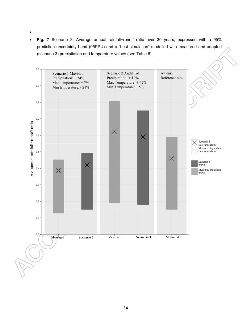
3.3.3 Scenario 3 (Precipitation & Temperature)
In scenario 3, average annual precipitation and minimum and maximum temperatures
were raised and lowered to a common level – that of Anjeni – for all three catchments
(Table 6). Looking at the 95PPU band the rainfall─runoff ratio in Andit Tid was 5%
higher in scenario 3 than in scenario 2, but decreased by almost 5% compared to the
simulation with measured precipitation and temperature. Due to higher temperatures in
scenario 3, the 10% higher precipitation rate did not lead to an increase in the
rainfall─runoff ratio (Fig. 7).
In Maybar, where the rainfall─runoff ratio was 10% higher in scenario 3, the increase
was smaller than in scenario 1. The reason is the higher potential evapotranspiration
rate, caused by a higher average annual temperature and a greater average diurnal
temperature variation (see equation 1), which was not considered in scenario 1. Overall,
in scenario 3 the hydrological responses of all three catchments are more similar to
each other than the hydrological responses calculated with the measured precipitation
and the simulated reference discharge of the different catchments (Table 6).
Due to percentage changes of the measured data in scenario 3, the rainfall pattern and
daily temperature fluctuations were still different in each catchment. Therefore, the
intensity as well as spatial and temporal distribution of precipitation in and between the
three catchments is still considerable and should not be neglected. For example, Andit
Tid, being more than four times as big as the two other catchments, had a greater risk
of unmonitored rainstorms and therefore displayed a wider range of possible runoff
responses than the two smaller catchments (Liu et al. 2008).

19
Despite these uncertainties, the changes in the rainfall─runoff ratio between the
scenarios proved the influence of precipitation and temperature on the hydrological
response. The differences between the three catchments in scenario 3, with the same
temperature and precipitation, showed the influence of other parameters which were not
used for scenario modelling. So “steep” slopes, like in Andit Tid and Maybar (average
slope: > 29%), and soils with a low infiltration capacity, like in Andit Tid (Liu et al. 2008),
generate more runoff than “gentle” slopes and deep soils, like in Anjeni (average slope:
19%). Differences in the hydrological responses between Andit Tid and Maybar, with
the same rainfall pattern, average slope, and growing season, can in addition be
explained by parameters which are directly influenced by humans, such as a higher
standard of soil and water conservation measures in Maybar (Hurni et al. 2005, Liu et
al. 2008).
Future hydrological responses will be highly dependent on the amplitude of the change
of precipitation and temperature. Both parameters have to be taken into account to
assess future blue and green water resources. Already small increases in precipitation
can lead to a disproportionately higher rainfall–runoff ratio, but increasing temperature
will convert blue to green water and decrease the amount of blue water for downstream
stakeholders, even if future temperature scenarios do not reach the amplitude of
scenario 2 and scenario 3.

20
4 SUMMARY AND CONCLUSION
In this study, we calculated the long-term hydrological responses of three small-scale
catchments with different hydrological and meteorological conditions. To do so, we used
the process-based semi-distributed hydrological model SWAT, carrying out calibration
and validation against measured discharge as well as sensitivity analysis, to simulate in
a first step a complete reference discharge time series for the three catchments. To
characterize the model’s uncertainty, we used SUFI-2 to generate a 95PPU band. In a
second step, we generated three scenarios, where we adapted the different
temperature and precipitation values of the three study regions to a common level. This
allowed us to compare hydrological responses of the three catchments under similar
meteorological conditions. Results show that increasing precipitation generates a
disproportionate increase of discharge and therefore a higher rainfall─runoff ratio, while
increasing temperature reduces the share of blue water for downstream countries.
These results indicated that differences in rainfall─runoff ratio and blue and green water
availability in catchments with different rainfall patterns are largely caused by
climatological parameters, such as precipitation and temperature. With the common
denominator (temperature and precipitation) we established a basis to compare the
effects of other parameters, such as land use change as well as soil and water
conservation practices. At the same time, a comparison of the scenarios we used and
different climate change scenarios showed that the impact of climate change on blue
and green water distribution depends on the combination of precipitation and
temperature change. Considering both parameters, many climate change scenarios will
lead to a higher share of blue water for downstream stakeholders, but also to more
green water in the headwaters, which can increase crop yield, when non-productive
evaporation is shifted to productive transpiration.
This study contributes to the as of yet scant body of knowledge on distribution and
availability of blue and green water in small-scale catchments with different rainfall
patterns. This knowledge is essential for assessing and improving watershed
management strategies for the long-term planning of local, national, and international
water, energy, and food security.

21
Acknowledgments
This research was supported by the Centre for Development and Environment (CDE),
and the Institute of Geography, University of Bern, Switzerland. We are grateful to the
Water and Land Resource Centre (WLRC), Addis Abeba, Ethiopia, for providing data,
and to Tina Hirschbuehl for editing.
Literature
Abbaspour, K.C., 2015. SWAT-CUP 2012: SWAT calibration and uncertainty programs - A user manual. Eawag: Swiss Federal Institute of Aquatic Science and Technology.
Abbaspour, K.C., van Genuchten, M.T., Schulin, R., and Schläppi, E., 1997. A sequential uncertainty domain inverse procedure for estimating subsurface flow and transport parameters. Water Resources Research, 33 (8), 1879–1892.
Abbaspour, K.C., Johnson, C.A., and van Genuchten, M.T., 2004. Estimating uncertain flow and transport parameters using a sequential uncertainty fitting procedure. Vadose Zone Journal, 3 (4), 1340–1352.
Abbaspour, K.C., Rouholahnejad, E., Vaghefi, S., Srinivasan, R., Yang, H., and Kløve, B., 2015. A Continental-Scale Hydrology and Water Quality Model for Europe: Calibration and uncertainty of a high-resolution large-scale SWAT model. Journal of Hydrology.
Abbaspour, K.C., Yang, J., Maximov, I., Siber, R., Bogner, K., Mieleitner, J., Zobrist, J., and Srinivasan, R., 2007. Modelling hydrology and water quality in the pre-alpine/alpine Thur watershed using SWAT. Journal of Hydrology, 333 (2-4), 413–430.
Abdo, K.S., Fiseha, B.M., Rientjes, T.H.M., Gieske, A.S.M., and Haile, A.T., 2009. Assessment of climate change impacts on the hydrology of Gilgel Abay catchment in Lake Tana Basin, Ethiopia. Hydrological Processes, 23, 3661–3669.
Adem, A.A., Tilahun, S.A., Ayana, E.K., Worqlul, A.W., Assefa, T.T., Dessu, S.B., and Melesse, A.M., 2016. Climate Change Impact on Stream Flow in the Upper Gilgel Abay Catchment, Blue Nile basin, Ethiopia. In: A.M. Melesse and W. Abtew, eds. Landscape Dynamics, Soils and Hydrological Processes in Varied Climates. Springer International Publishing, 645–673.
Ali, Y.S.A., Crosato, A., Mohamed, Y.A., Abdalla, S.H., and Wright, N.G., 2014. Sediment balances in the Blue Nile River Basin. International Journal of Sediment Research, 29 (3), 316–328.
Andersen, J., Refsgaard, J.C., and Jensen, K.H., 2001. Distributed hydrological modelling of the Senegal River Basin — model construction and validation. Journal of Hydrology, 247 (3-4), 200–214.
Arnold, J.G., Allen, P.M., Muttiah, R., and Bernhardt, G., 1995. Automated Base Flow Separation and Recession Analysis Techniques. Ground Water, 33 (6), 1010–1018.
Arnold, J.G., Moriasi, D.N., Gassman, P.W., Abbaspour, K.C., White, M.J., Srinivasan, R., Santhi, C., Harmel, R.D., van Griensven, A., Van Liew, M.W., Kannan, N., and Jha, M.K., 2012. SWAT: Model use, calibration, and validation. Transactions of the ASABE, 55(4), 1491–1508.
Awulachew, S.B., McCartney, M., Steenhuis, T.S., and Ahmed, A.A., 2009. A review of hydrology,

22
sediment and water resource use in the Blue Nile Basin. Working Paper 131. International Water Management Institute (IMWI).
Bayabil, H.K., Tilahun, S.A., Collick, A.S., Yitaferu, B., and Steenhuis, T.S., 2010. Are runoff processes ecologically or topographically driven in the (sub) humid Ethiopian highlands? The case of the Maybar watershed. Ecohydrology, 3 (4), 457–466.
Betrie, G.D., Mohamed, Y.A., van Griensven, A., and Srinivasan, R., 2011. Sediment management modelling in the Blue Nile Basin using SWAT model. Hydrology and Earth System Sciences, 15 (3), 807–818.
Bono, R. and Seiler, W., 1984. The Soils of the Andit-Tid Research Unit (Ethiopia) Classification, Morphology and Ecology, with soil map 1:10’000. University of Bern, Switzerland.
Bosshart, U., 1997. Catchment discharge and suspended sediment transport as indicators of physical soil and water conservation in the Michet catchment, Anjeni Research Unit. A case study in the north-western Highlands of Ethiopia. University of Berne, Switzerland.
Bosshart, U., 1999. Hydro-sedimentological characterisation of Kori Sheleko and Hulet Wenz Catchments, Maybar and Andit Tid research units: Case studies of two SCRP micro-catchments in the north-eastern highlands of Ethiopia. University of Berne, Switzerland.
Brandsma, J., van den Eertwegh, G.A.P., Droogers, P., Bai, Z., and Zhang, S., 2013. Green and Blue Water R esources and Management Scenarios using the SWAT model for the Upper Duhe Basin, China - Feasibility Study. Report FutureWater 126. Wageningen, Netherlands.
Collick, A.S., Easton, Z.M., Ashagrie, T., Biruk, B., Tilahun, S., Adgo, E., Awulachew, S.B., Zeleke, G., and Steenhuis, T.S., 2009. A simple semi-distributed water balance model for the Ethiopian highlands. Hydrological Processes, 23 (26), 3718–3727.
Dile, Y.T., Berndtsson, R., and Setegn, S.G., 2013. Hydrological Response to Climate Change for Gilgel Abay River, in the Lake Tana Basin - Upper Blue Nile Basin of Ethiopia. PloS one, 8 (10), e79296.
Dile, Y.T. and Srinivasan, R., 2014. Evaluation of CFSR climate data for hydrologic prediction in data-scarce watersheds: an application in the Blue Nile River Basin. Journal of the American Water Resources Association, 50 (5), 1226–1241.
Engel, B., Storm, D., White, M., Arnold, J.G., and Arabi, M., 2007. A Hydrologic/Water Quality Model Application Protocol. Journal of the American Water Resources Association, 43 (5), 1223–1236.
Enku, T., Melesse, A.M., Ayana, E.K., Tilahun, S.A., Zeleke, G., and Steenhuis, T.S., 2016. Watershed Storage Dynamics in the Upper Blue Nile Basin: The Anjeni Experimental Watershed, Ethiopia. In: A.M. Melesse and W. Abtew, eds. Landscape Dynamics, Soils and Hydrological Processes in Varied Climates. Springer International Publishing, 261–277.
Faramarzi, M., Abbaspour, K.C., Ashraf Vaghefi, S., Farzaneh, M.R., Zehnder, A.J.B., Srinivasan, R., and Yang, H., 2013. Modeling impacts of climate change on freshwater availability in Africa. Journal of Hydrology, 480, 85–101.
Faramarzi, M., Abbaspour, K.C., Schulin, R., and Yang, H., 2009. Modelling blue and green water resources availability in Iran. Hydrological Processes, 23 (3), 486–501.
Fuka, D.R., Walter, M.T., MacAlister, C., Degaetano, A.T., Steenhuis, T.S., and Easton, Z.M., 2014. Using the Climate Forecast System Reanalysis as weather input data for watershed models. Hydrological Processes, 28 (22), 5613–5623.
Gassman, P.W., Reyes, M.R., Green, C.H., and Arnold, 2007. The Soil and Water Assessment Tool: Historical development, applications, and future research directions. Center for Agricultural and Rural Development, Iowa State University, Iowa.
Gebre, S.L., Tadele, K., and Mariam, B.G., 2015. Potential Impacts of Climate Change on the Hydrology

23
and Water resources Availability of Didessa Catchment, Blue Nile River Basin, Ethiopia. Journal of Geology & Geosciences, 4 (1), 193.
Gessesse, B., Bewket, W., and Bräuning, A., 2014. Model-based characterization and monitoring of runoff and soil erosion in response to land use/land cover changes in the Modjo watershed, Ethiopia. Land Degradation & Development.
van Griensven, A., Ndomba, P., Yalew, S., and Kilonzo, F., 2012. Critical review of the application of SWAT in the upper Nile Basin countries. Hydrology and Earth System Sciences Discussions, 9 (3), 3761–3788.
Hagosa, F., Makombe, G., Namara, R., and Awulachew, S., 2011. Importance of Irrigated Agriculture to the Ethiopian Economy: Capturing the direct net benefits of irrigation. Ethiopian Journal of Development Research, 32 (1), 1–37.
Hargreaves, G.L., Hargreaves, G.H., and Riley, J.P., 1985. Agricultural Benefits for Senegal River Basin. Journal of Irrigation and Drainage Engineering, 111 (2), 113–124.
Hurni, H., 1998. Agroecological Belts of Ethiopia Explanatory notes on three maps at a scale of 1:1,000,00. Soil Conservation Research Programme, Research Report 43. Bern, Switzerland: Centre for Development and Environment (CDE).
Hurni, H., Tato, K., and Zeleke, G., 2005. The Implications of Changes in Population, Land Use, and Land Management for Surface Runoff in the Upper Nile Basin Area of Ethiopia. Mountain Research and Development, 25 (2), 147–154.
Kejela, K., 1995. The soils of the Anjeni Area - Gojam Research Unit, Ethiopia. University of Bern, Switzerland.
Kim, U. and Kaluarachchi, J.J., 2009. Climate Change Impacts on Water Resources in the Upper Blue Nile River Basin, Ethiopia. Journal of the American Water Resources Association, 45 (6), 1361–1378.
Koch, M. and Cherie, N., 2013. SWAT-Modeling of the Impact of future Climate Change on the Hydrology and the Water Resources in the Upper Blue Nile River Basin, Ethiopia. Proceedings of the 6th International Conference on Water Resources and Environment Research, ICWRER, 6 (6), 488–523.
Krause, P., Boyle, D.P., and Bäse, F., 2005. Comparison of different efficiency criteria for hydrological model assessment. Advances in Geosciences, 5 (5), 89–97.
Lin, S., Jing, C., Chaplot, V., Yu, X., Zhang, Z., Moore, N., and Wu, J., 2010. Effect of DEM resolution on SWAT outputs of runoff, sediment and nutrients. Hydrology and Earth System Sciences Discussions, 7 (4), 4411–4435.
Liu, B.M., Collick, A.S., Zeleke, G., Adgo, E., Easton, Z.M., and Steenhuis, T.S., 2008. Rainfall-discharge relationships for a monsoonal climate in the Ethiopian highlands. Hydrological Processes, 22 (7), 1059–1067.
Mbonimpa, E.G., 2012. SWAT Model Application to Assess the Impact of Intensive Corn-farming on Runoff, Sediments and Phosphorous loss from an Agricultural Watershed in Wisconsin. Journal of Water Resource and Protection, 04 (07), 423–431.
Melesse, A., Abtew, W., and Setegn, S.G., 2014. Nile River Basin: Ecohydrological Challenges, Climate Change and Hydropolitics. Springer Science & Business Media.
Mengistu, D.T. and Sorteberg, A., 2011. Validation of SWAT simulated streamflow in the Eastern Nile and sensitivity to climate change. Hydrology and Earth System Sciences Discussions, 8 (5), 9005–9062.
Moriasi, D.N., Arnold, J.G., Van Liew, M.W., Bingner, R.L., Harmel, R.D., and Veith, T.L., 2007. Model evaluation guidelines for systematic quantification of accuracy in watershed simulations. Trans. ASABE, 50 (3), 885–900.

24
Pascual, D., Pla, E., Lopez-Bustins, J.A., Retana, J., and Terradas, J., 2014. Impacts of climate change on water resources in the Mediterranean Basin: a case study in Catalonia, Spain. Hydrological Sciences Journal, 141217125340005.
Ritchie, J.T., 1972. Model for predicting evaporation from a row crop with incomplete cover. Water Resources Research, 8 (5), 1204–1213.
Rockström, J., 2003. Water for food and nature in drought-prone tropics: vapour shift in rain-fed agriculture. Philosophical transactions of the Royal Society of London. Series B, Biological sciences, 358 (1440), 1997–2009.
Roth, V. and Lemann, T., 2016. Comparing CFSR and conventional weather data for discharge and soil loss modelling with SWAT in small catchments in the Ethiopian Highlands. Hydrology and Earth System Sciences, 20 (2), 921–934.
Schuol, J. and Abbaspour, K.C., 2007. Using monthly weather statistics to generate daily data in a SWAT model application to West Africa. Ecological Modelling, 201 (3-4), 301–311.
Schuol, J., Abbaspour, K.C., Srinivasan, R., and Yang, H., 2008a. Estimation of freshwater availability in the West African sub-continent using the SWAT hydrologic model. Journal of Hydrology, 352 (1-2), 30–49.
Schuol, J., Abbaspour, K.C., Yang, H., Srinivasan, R., and Zehnder, A.J.B., 2008b. Modeling blue and green water availability in Africa. Water Resources Research, 44 (7).
Setegn, S.G., Dargahi, B., Srinivasan, R., and Melesse, A.M., 2010. Modeling of Sediment Yield From Anjeni-Gauged Watershed, Ethiopia Using SWAT Model. Journal of the American Water Resources Association, 46 (3), 514–526.
Setegn, S.G., Srinivasan, R., and Dargahi, B., 2008. Hydrological Modelling in the Lake Tana Basin, Ethiopia Using SWAT Model. The Open Hydrology Journal, 2 (1).
Setegn, S.G., Srinivasan, R., Dargahi, B., and Melesse, A.M., 2009. Spatial delineation of soil erosion vulnerability in the Lake Tana Basin, Ethiopia. Hydrological Processes, 24 (3), 357–367.
Steenhuis, T.S., Collick, A.S., Easton, Z.M., Leggesse, E.S., Bayabil, H.K., White, E.D., Awulachew, S.B., Adgo, E., and Ahmed, A.A., 2009. Predicting discharge and sediment for the Abay (Blue Nile) with a simple model. HYDROLOGICAL PROCESSES, 23 (26), 3728–3737.
Steenhuis, T.S., Hrnčíř, M., Poteau, D., Romero Luna, E.J., Tilahun, S.A., Caballero, L.A., Guzman, C.D., Stoof, C.R., Šanda, M., Yitaferu, B., and Císlerová, M., 2013. A Saturated Excess Runoff Pedotransfer Function for Vegetated Watersheds. Vadose Zone Journal, 12 (4).
Stehr, A., Debels, P., Arumi, J.L., Romero, F., and Alcayaga, H., 2009. Combining the Soil and Water Assessment Tool (SWAT) and MODIS imagery to estimate monthly flows in a data-scarce Chilean Andean basin. Hydrological Sciences Journal, 54 (6), 1053–1067.
Stehr, A., Debels, P., Romero, F., and Alcayaga, H., 2008. Hydrological modelling with SWAT under conditions of limited data availability: evaluation of results from a Chilean case study. Hydrological Sciences Journal, 53 (3), 588–601.
Taye, M.T., Ntegeka, V., Ogiramoi, N.P., and Willems, P., 2011. Assessment of climate change impact on hydrological extremes in two source regions of the Nile River Basin. Hydrology and Earth System Sciences, 15 (1), 209–222.
Taye, M.T., Willems, P., and Block, P., 2015. Implications of climate change on hydrological extremes in the Blue Nile basin: A review. Journal of Hydrology: Regional Studies, 4, 280–293.
Tebebu, T.Y., Steenhuis, T.S., Dagnew, D.C., Guzman, C.D., Bayabil, H.K., Zegeye, A.D., Collick, A.S., Langan, S., MacAlister, C., Langendoen, E.J., Yitaferu, B., and Tilahun, S.A., 2015. Improving efficacy of landscape interventions in the (sub) humid Ethiopian highlands by improved understanding of

25
runoff processes. Frontiers in Earth Science, 3. Tekleab, S., Uhlenbrook, S., Savenije, H.H.G., Mohamed, Y., and Wenninger, J., 2015. Modelling rainfall–
runoff processes of the Chemoga and Jedeb meso-scale catchments in the Abay/Upper Blue Nile basin, Ethiopia. Hydrological Sciences Journal, 1–18.
Tibebe, D. and Bewket, W., 2011. Surface runoff and soil erosion estimation using the SWAT model in the Keleta Watershed, Ethiopia. Land Degradation & Development, 22 (6), 551–564.
Tilahun, S.A., Guzman, C.D., Zegeye, A.D., Engda, T.A., Collick, A.S., Rimmer, A., and Steenhuis, T.S., 2013a. An efficient semi-distributed hillslope erosion model for the subhumid Ethiopian Highlands. Hydrology and Earth System Sciences, 17 (3), 1051–1063.
Tilahun, S.A., Mukundan, R., Demisse, B.A., Engda, T.A., Guzman, C.D., Tarakegn, B.C., Easton, Z.M., Collick, A.S., Zegeye, A.D., Schneiderman, E.M., Parlange, J.-Y., and Steenhuis, T.S., 2013b. A Saturation Excess Erosion Model. Transactions of the ASABE, 56 (2), 681–695.
Weigel, G., 1986. The Soils of the Maybar Area, Wello Research Unit, Ethiopia. University of Bern, Switzerland.
White, K.L. and Chaubey, I., 2005. Sensitivity Analysis, Calibration, and Validations for a Multisite and Multivariable SWAT Model. Journal of the American Water Resources Association, 41 (5), 1077–1089.
WLRC, 2015. Water and Land Resources Information System (WALRIS) [online]. Available from: http://walris.wlrc-eth.org/ [Accessed 15 Dec 2015].
Zeleke, G., 2000. Landscape Dynamics and Soil Erosion Process Modeling in the North-Western Ethiopian Highlands. African Studies Series A 16. Geographica Bernensia, Bern, Switzerland.

26
Table 1 Information on the three small-scale catchments
Andit Tid Maybar Anjeni
Location of gauging station 9.815°N, 37.711°E 10.996°N, 39.657°E 10.678°N, 37.530°E
Area of hydrological catchmenta 477.3 ha 112.8 ha 113.4 ha
Area as calculated with SWAT 474.4 ha 104.7 ha 106.56ha Altitudinal rangea 3040-3548 m asl 2530-2858 m asl 2406-2507 m asl
Average slope 29.4% 29.5% 19.0%
Rainfall pattern Bimodal Bimodal Unimodal
Growing seasona 175 d 175 d 242 d
Major soilsa Andosols, Fluvisols, Regosols, Lithosols
Phaeozems, Lithosols, Gleysols
Alisols, Nitosols, Cambisols
Average annual min /max temperatureb 8.2°C / 8.6°C 10.9°C / 21.7°C 8.6°C / 23.3°C
Average annual rainfallb 1542 mm 1363 mm 1698 mm
Average annual dischargeb 816 mm 369 mm 766 mm
Average annual rainfall–runoff ratioc 0.59 0.29 0.46 a=SCRP (Bosshart 1997, 1999, Hurni 1998)
b=WLRC (2015) c=Average of years with available precipitation and discharge data

27
Table 2 Available weather data and calibration/validation periods
Andit Tid Maybar Anjeni Precipitation and temperature 1982-2013 1981-2002, 2004-2013 1985-2002, 2004-2013
Discharge 1982-1997
1982-1989, 1992-1993, 1995-1998, 2001-2004,
2006, 2008-2009, 2012-2013
1984-1998, 2010, 2012-2013
Calibration period 1985-1993 1984-1998 1986-1998
Validation period 1994-1997 2001-2013 2010-2013
Notes: Individual years are not complete. If data of 6 or more months per year were available, the year is listed.
Table 3 Description of input parameters selected for scenario modelling
Parameter Name Description Maybar Andit Tid
Scen 1 Scen 3 Scen 2 Scen 3
r__Precipitation.pcp Amount of precipitation falling during the day (mm) 0.24 0.24 --- 0.1
r__PCPMM.wgna Average or mean total monthly precipitation (mm) 0.24 0.24 --- 0.1
r__RAINHHMX.wgna Max. 0.5 hour rainfall in entire period of record for month (mm) 0.24 0.24 --- 0.1
r__PCPSTD.wgna Standard deviation for daily precipitation in month (mm/d) 0.24 0.24 --- 0.1
r__TMPMX.wgna Average daily max. air temperature for month (ºC). --- 0.07 0.42 0.42
r__TMPMN.wgna Average daily min. air temperature for month (ºC). --- -0.21 0.05 0.05
r__MAXTEMP.tmp Daily maximum temperature (ºC) --- 0.07 0.42 0.42
r__MINTEMP.tmp Daily minimum temperature (ºC) --- -0.21 0.05 0.05
r_TMPSTDMX.wgna Standard deviation for daily max. air temperature in month (ºC) --- 0.07 0.42 0.42
r_TMPSTDMN.wgna Standard deviation for daily min. air temperature in month (ºC) -0.21 0.05 0.05 Note: In the parameter names, r__ means the existing parameter value is multiplied by (1 + a given value) (Abbaspour 2015). aRequired for the weather generator (to fill in gaps when measured data is missing).

28
Table 4 Description of input parameters selected for calibration, and final parameter ranges after calibration of discharge.
Parameter Name Description Andit Tid Maybar Anjeni
Min Max Min Max Min Max
a__CN2.mgt SCS runoff curve number for moisture condition 2 -10a 10a -10 10 -10 10
v__GW_DELAY.gw Groundwater delay (d) 30 100 50 200 30 150
v__GWQMN.gw Threshold depth of water in the shallow aquifer required for return flow to occur (mm).
50 200 0 200 50 200
v__ESCO.hru Soil evaporation compensation factor. 0.6 1 0.7 1 0.6 0.9
v__GW_REVAP.gw Groundwater "revap" coefficient 0.1 0.2 0.1 0.2 0.1 0.2
v__REVAPMN.gw Threshold depth of water in the shallow aquifer for "revap" to occur (mm)
0 10 0 8 4 10
v__CH_K2.rte Effective hydraulic conductivity in main channel alluvium
0.1 130 1 150 0.1 130
v__CH_N2.rt Manning's "n" value for the main channel 0 0.3 0 0.3 0 0.3
v__SURLAG.bsn Surface runoff lag time (d) 0.05 1 0.05 0.9 0.05 1
v__RCHRG_DP.gw Deep aquifer percolation fraction 0 1 0.2 1 0 1
v__EPCO.hru Plant uptake compensation factor 0 1 0.1 0.7 0 1
r__OV_N.hru Manning’s n value for overland flow -0.2 0.2 -0.2 0.1 -0.1 0.2 Note: In the parameter names, a__ means the given value is added to the existing parameter value; r__ means the existing parameter value is multiplied by (1 + a given value); v__ means the existing parameter value is to be replaced by the given value (Abbaspour 2015). aCN2 already adjusted during the modelling process with SWAT (+15)
Table 5 Final calibration and validation statistics for the three small-scale catchments
P-factor R-factor R2 NSE Calibration Validation Calibration Validation Calibration Validation Calibration ValidationAndit Tid 0.84 0.79 0.58 0.79 0.83 0.73 0.8 0.68
Maybar 0.75 0.83 0.77 0.79 0.74 0.78 0.65 0.66
Anjeni 0.81 0.81 0.85 0.77 0.93 0.89 0.93 0.88
Table 6 Temperature, precipitation, potential evapotranspiration (PET), and annual rainfall─runoff ratio for scenarios 1-3
Maybar Andit Tid Anjeni
Referencea Scenario 1 Scenario 3 Referencea Scenario 2 Scenario 3 Referencea
Av. annual min temperature (°C) 10.9 10.9 8.6 8.2 8.6 8.6 8.6
Av. annual max temperature (°C) 21.7 21.7 23.3 16.4 23.3 23.3 23.3
Av. annual precipitation (mm) 1363 1698 1698 1542 1542 1698 1698
Av. annual PET (mm)b 1330 1330 1453 1099 1608 1608 1505
Av. annual rainfall–runoff ratio 0.38 0.46 0.42 0.62 0.57 0.59 0.46 aReference values are measured (temperature and precipitation) or simulated (rainfall–runoff ratio) using the best simulation value from the calibration process.bPotential Evapotranspiration (PET) is calculated using the Hargreaves Method (Hargreaves et al. 1985).

29
• Fig. 1 Map overview of the Upper Blue Nile Basin in the Ethiopian Highlands with the WLRC
observatories, and the agro-ecological zones according to Hurni (1998)

30
•
• Fig. 2 Rainfall distribution in Andit Tid, Maybar, and Anjeni (WLRC 2015)
•
• Fig. 3 Discharge calibration and validation of all three catchments.
0
200
400
600
800
Jan
FebMar
AprMay
Jun Ju
lAug
SepOct
NovDec
Prec
ipita
tion
[mm
]
Monthly precipitation distribution Andit Tid (1982−2013)
0
200
400
600
800
Jan
FebMar
AprMay
Jun Ju
lAug
SepOct
NovDec
Monthly precipitation distributionMaybar (1981−2013)
0
200
400
600
800
Jan
FebMar
AprMay
Jun Ju
lAug
SepOct
NovDec
Monthly precipitation distribution Anjeni (1985−2013)
0.0
0.2
0.4
0.6
0.8
1.0
1.2
1.4
19851986
19871988
19891990
19911992
1993
Calibration Andit Tid
0.0
0.2
0.4
0.6
0.8
1.0
1.2
1.4
19941995
19961997
Validation Andit Tid
0.00
0.05
0.10
0.15
19841985
19861987
19881989
19921993
19951996
19971998
Calibration Maybar
0.00
0.05
0.10
0.15
20012002
20032004
20062008
20092011
20122013
Validation Maybar
0.00
0.05
0.10
0.15
19861987
19881989
19901991
19921993
19941995
19961997
1998
Calibration Anjeni
0.00
0.05
0.10
0.15
20102012
2013
Validation Anjeni
95PPU Best Sim Observed
Dis
char
ge m
3/s

31
Fig. 4 Average annual and monthly rainfall─runoff ratio with a trend line for all data. Years and months with no measured data have been simulated with the best simulation value from the calibration process (values >1 = 1). The SWAT warm-up periods (the first 2 years) have been skipped.
0.2
0.4
0.6
0.8
1.0
1986 1990 1994 1998 2002 2006 2010 2014
Ann
ual r
ainf
all-r
unoff
ratio
Andit Tid
0.2
0.4
0.6
0.8
1.0
1986 1990 1994 1998 2002 2006 2010 2014
Maybar
0.2
0.4
0.6
0.8
1.0
1986 1990 1994 1998 2002 2006 2010 2014
Anjeni
0.2
0.4
0.6
0.8
1.0
1986 1990 1994 1998 2002 2006 2010 2014
May
0.2
0.4
0.6
0.8
1.0
1986 1990 1994 1998 2002 2006 2010 2014
May
0.2
0.4
0.6
0.8
1.0
1986 1990 1994 1998 2002 2006 2010 2014
May
0.2
0.4
0.6
0.8
1.0
1986 1990 1994 1998 2002 2006 2010 2014Mon
thly
rain
fall-
runo
ff ra
tio
June
0.2
0.4
0.6
0.8
1.0
1986 1990 1994 1998 2002 2006 2010 2014
June
0.2
0.4
0.6
0.8
1.0
1986 1990 1994 1998 2002 2006 2010 2014
June
0.2
0.4
0.6
0.8
1.0
1986 1990 1994 1998 2002 2006 2010 2014
July
0.2
0.4
0.6
0.8
1.0
1986 1990 1994 1998 2002 2006 2010 2014
July
0.2
0.4
0.6
0.8
1.0
1986 1990 1994 1998 2002 2006 2010 2014
July
0.2
0.4
0.6
0.8
1.0
1986 1990 1994 1998 2002 2006 2010 2014
August
0.2
0.4
0.6
0.8
1.0
1986 1990 1994 1998 2002 2006 2010 2014
August
0.2
0.4
0.6
0.8
1.0
1986 1990 1994 1998 2002 2006 2010 2014
August
95PPU measured data best simulation

32
Fig. 5 Scenario 1: Average annual rainfall−runoff ratio over 30 years; expressed with a 95%
prediction uncertainty band (95PPU) and a “best simulation” modelled with measured and adapted
(scenario 1) precipitation and temperature values (see Table 6).
0.0
0.1
0.2
0.3
0.4
0.5
0.6
0.7
0.8
0.9
1.0
Av.
ann
ual r
ainf
all−
runo
ff ra
tio
Scenario 1Best simulation
Scenario 195PPU
Scenario 1 Maybar:Precipitation: + 24%
Anjeni:Reference site
Measured input data Best simulation
Measured Scenario 1 Measured
Measured input data 95PPU

33
•
• Fig. 6 Scenario 2: Average annual rainfall−runoff ratio over 30 years; expressed with a 95%
prediction uncertainty band (95PPU) and a “best simulation” modelled with measured and adapted
(scenario 2) precipitation and temperature values (see Table 6).
0.0
0.1
0.2
0.3
0.4
0.5
0.6
0.7
0.8
0.9
1.0
Measured Scenario 2 Measured
Av.
ann
ual r
ainf
all−
runo
ff ra
tio
Anjeni:Reference site
Scenario 2 Andit Tid:Max Temperature: + 42%Min Temperature: + 5%
Scenario 2Best simulation
Scenario 295PPU
Measured input data Best simulation
Measured input data 95PPU
34
•
• Fig. 7 Scenario 3: Average annual rainfall−runoff ratio over 30 years; expressed with a 95%
prediction uncertainty band (95PPU) and a “best simulation” modelled with measured and adapted
(scenario 3) precipitation and temperature values (see Table 6).
0.0
0.1
0.2
0.3
0.4
0.5
0.6
0.7
0.8
0.9
1.0
Av.
ann
ual r
ainf
all−
runo
ff ra
tio
Scenario 1 Maybar:Precipitation: + 24%Max temperature: + 7%Min temperature: - 21%
Measured Scenario 3 Measured Scenario 3 Measured
Anjeni:Reference site
Scenario 2 Andit Tid:Precipitation: + 10%Max Temperature: + 42%Min Temperature: + 5%
Scenario 3Best simulation
Scenario 395PPU
Measured input data Best simulation
Measured input data 95PPU