Y

PARALLEL DOMAIN DECOMPOSXTION FORMULATION AND SOFTWARE FOR

APPLICATIONS LARGE-SCALE SPARSE SYMMETRICAL/UNSY’I\IMETRICAL AEROACOUSTIC

By:

D.T. NGUYEN

Final Report For the Period January 15.2001 - January 14,2005

Prepared for National Aeronautics and Space Administration Langley Research Center Hampton, Virginia 2368 1

ODU

Technical Monitor and Collaborator Dr. Willie R. Watson (NASA LaRC)

https://ntrs.nasa.gov/search.jsp?R=20050123564 2018-05-13T06:38:05+00:00Z

1. introduction

The overall objectives of this research work are to formulate

and validate efficient parallel algorithms, and to efficiently

desigdimplement computer software for solving large-scale

acoustic problems, arised from the unified frameworks of the

finite element procedures.

The adopted parallel Finite Element (E) Domain Decomposition (DD)

procedures should fully take advantages of multiple processing

capabilities offered by most modern high performance computing

platforms for efficient parallel computation. To achieve this

objective. the formulation needs to integrate efficient sparse

(and dense) assembly techniques (see Section 2), hybrid (or mixed)

direct and iterative equation soh-ers (see Section 3), proper

pre-conditioned strategies, unrolling strategies [Ref. 6.5, Chapter lo],

and effective processors' communicating schemes (see Section 3).

Finally, the numerical performance of the developed parallel

finite element procedures will be evaluated by solving series of

structural, and acoustic (symmetrical and un-symmetrical) problems

(in different computing platforms). Comparisons with existing

"commercialized" [Ref. 6.101 andor "public domain" [Ref. 6.1 13

software are also included, whenever possible.

2. Algorithms and Application of Sparse Matrix Assembly and Equation Solvers for Aeroacoustics [Ref. 6.11

(Please refer to the attached Journal Paper for this section)

2

Algorithms and Application of Sparse Matrix Assembly . and Equation Solvers for Aeroacoustics

W. R. Watson* NASA Langley Research Cenrer. Hanipton, \ i'rginia 23681

D. T. Npyen' Old Dotiiiriiori I'iiii.ersiF. Norfolk, ISrgirria 235-79

C. J. Reddy' EM. I t i c .. H ~ i ~ i p ~ o i i . \irginia 13666

v. N. Vatsa" NASA Luiiglex Research Cenrer, Hamproti. i'r3inia 23681

and W. H. Tang'

Hang Kotig Ctiiwrsip of Scictrcc mid Tccivlolos!, Kowloon. Horig Kong. People's Republic of Chiria

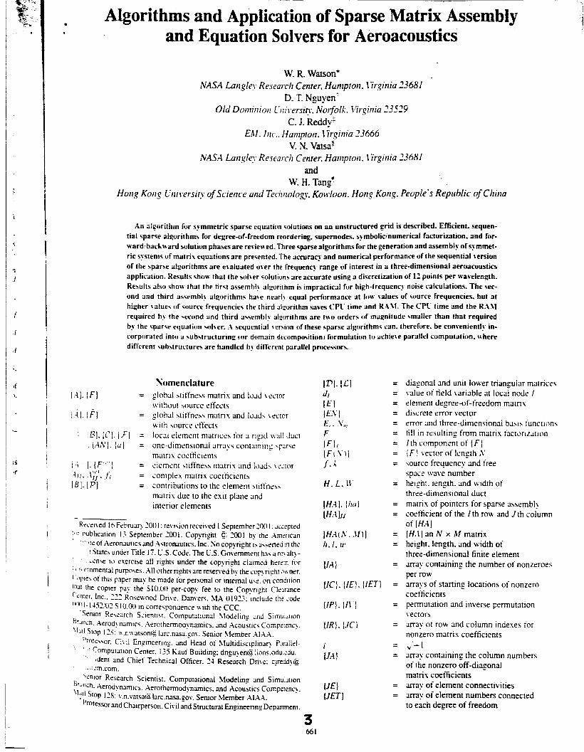
Aii alguiiiiun for symmetric sparse equaticin wiutions on an unstructured grid is described. Efficient. sequen- tial sparse algorithm4 for degree-of-freedom reordering. supernodes. synbolictnumerical factorization. and for- ward+ackaard solution phases are reviewed. Three sparse algorithms for the generation and assemblv of sFmmet- ric systems of matri\ equations are prewnted. The amrac? and numerical performance of the sequential version of the rparse algorithms are evaluated oier the frequency range of interest in a three-dimensional aeroacoustics application. Results show that the soher solution4 are accurate using a discretization of 12 points per wavelength. Rewits also 4hou that the tirst assemhl! algorirhm is impractical for high-frequenc! noise calculations. The 4ec- ond and third assemhl! algorithms ha\e nearl? equal performance at lou d u e s of source frquencies. but at higher \alue4 of wurce frequencies the third deorithm saves CPC' time and RAW The CPL time and the R.411 required h! the wxmnd and third ashemhi! aleurithmc are orders of magnitude *mailer than that required b! the sparw equation \ol\er. .\ sequential \ errion of these sparse algorithms can. therefore. be conveniently in- corpcirated into a \ub*tructuring tor domain decompmitioni formulation to achiete parallel computation. \\here diffcrent whstructures are handld I)! different parallel priwwirs.

Sumenclature 1.41. IF1 = glohal hriffnehc matrix and load iector

i . i / . I F ] = global d f n w matrix and load, \ectcr ui thout bource effects

N ith rource effects : ; E ] . IC']. IF] = local dement niatricch for I rigid \\ai! duct

. {An'). {ul = one-dirnemional arrays containing main\ cocfticients

= rlemcnr stiffnrhs matrix and load\ \siror ~ .{ ' 1. IF'''') A / / . .I;'. t / = complex matris coefticients I I . IF1 = contributions to the element rtiifneh\

marrix due to the exit plane and interior elements

Rzceived I h Fcbruar! 2001 : revwon received I Septemher 200 I . x x p t e d mblicaiion 1.7 September 2001. Copyright c; 2001 by the .Am:rican

' ' ' . ! !e of Aeronautics and .Ammauiics. Inc. So copyright I \ ;I,\cmea :n the ! Stares under Title 17. C.S. Code. The U.S. Government h35 a re! ;111! - dnse to exercise a11 righrr under the copyright claimed herein tor ' ' mnenral purpose%. All orher righrc are resened by the cop! righi wner.

(-llPle\ of this p3ptr m y be made for per.;onal or internal ux. on condition IhJl the copier the jlO.[!O per-copy fee to the Copyright Clc;lr;Ince ('mer. Inc.. 2 2 RoIewnod Dri\e. Darners. S1X 01921: include th: :ode 'q"11-14S?~02 510.00 in correspondence \\ith the CCC.

' Senior Rerezrch Scienricr. Computarional Slodclin, 0 Jnd Siiiudiion 9raili.h. Aerod! narnic5. .Aerothermodynamics. and .~coustics Cornpe::nc!. ''a1 slop 12s: v. .r.\\atsor@ Iarc.nasa.gov. Senior Sfrmber .Il.A.A.

Prnfe\\or. ci\ 1 1 Engineenng and Head of ~lulridiscipi~nap Pmilel- ''

' " fomPutJrion Center. I35 Kaui Building: dngu>en(ij liclns.odu.cdu. dent and Chief Technical Officer. 24 Research Dme: cJreaa!@ m.com.

h l o r Re5earch Scientist. Computational SIodelin, 0 and Sirnulation Hr.lnih. Aerodynamics. Aerothermodynamics. and Acoustics Cornpermy. ''ill Stop 128: v.n.vatsa(g 1arc.nasa.gov. Seruor ilemter XI.A.A.

''rotemrand Chairperson. Civil and Structuural Engineenng Department.

' . .

H . L. II

IIRI. IJCl

1

(J.4 I

= diagonal and unit lower triangular matrices = value of held variable at local node I = element degrcr-of-freedom man\ : = discrete error vector = error and three-dimensional barn t'unctiont = t i l l in resulting from matril tactorir.mon = I th component of 1 f 1 = ( F ) vector of lcngth A' = \ourcc frequency and free

space wave number = height. length. and width of

three-dimensional duct = matrix of pointers for sparse assembl! = coefficient of the I th row and J t h column

of [ H A J = [ H A ] an N x M matrix = height. length. and width of

three-dimensional finite element = m a y containing the number of nonzeroe.;

per row = m a y s of starting locations of nonzero

coetticients = permutation and inverse permutation

\ectors = array of row and column indexes for

nonzero matrix coefficients

= m a y containing the column numbers of the nonzero off-diagonal matrix coefficients

= amy of element connectivities = a m y of element numbers connected

to each degree of freedom

= .-I

3 66 1

W- ..,....- ..

M *

. ME

(MP]

N

,V€. .SP

S F

;v 1

P p,. . p .

Reierr. id,,

s . t ' ,\

SIlntr"pf'

r . R FF. BB 1 . J

exit. .\

5iipc.rtr.ripr.c

1'

1 . . I . K 7 x.

number of n~NerO coefficients in a sparse manix. N + N l maximum number of elements connected to a degree of freedom array of element numbers connected to a degree of freedom array containing the number of elements connected to a degree of freedom master degree-of-freedom m a \ maximum number of nonzero coefficients per row number of unknowns in the nnirc element discretization number of finite elements and degrees of freedom per element number of fi l l ins during factonzation of a matrix total number of transverse. spanwise. and axial nodes number of nonzero. off-diagonal coefticients before factonzation number of nonzero. off-diagonal coefticients after factorization acoustic pressure tield acoustic pressure at local node w 2nd source pressure relative error norm and uniiomi 110n \peed surface and voiume of a tiniie eiemmt nonzero value that \va\ modined during matrix factorization Cartesian coordinates transverse. spanwise. and axial 1oi.itions of grid lines dimensionless esit admittance derivative of the acoustic preswre normal to 3 suriace dimensittiiles\ \tall and esit impcdance global vector of unknowns local vectors of unknowns intermediate ectors for fomard and backward submution vector componcnts gradient vector and Laplace operator vector dot product

exit and source plane index factored and reordered matnx forward and backward substitution rou and column index of 3 matnx

truss element number gnd line locator tor three-dimenslonal duct matnx or vector transpose complex conjugate

I. Introduction HREE-DIMENSIOSXL aeroacoustics codes that can ~ C C U - T ratel!. predict the noise radiated from commerciai aircraft are

needed.! Currently. noise prediction codes require the use of a linear equation solver before radiated noise can be predicted. An optimizer must then run the noise predictive code on a digital computer hun- dreds of times IO achieve an aircraft design with a minimal noise radiation signature.

Currently. industry and government aircraft noise predictive codes are either two-dimensional or treat only axisymmeuic noise signatures.' When the volumes are three-dimensional. the currently used equation solvers require an excessive amount of CPU time

low-frequency sound sources in two-dimensional or axisjmmetri,- environments.

Sparse equation solving technologies'-" have been &veloFs, and are well documented for several engineering applications. -r. .: the computational advantage of sparse solver technology o,e. :. more conventional rechnologies (such as band or skyline sOi . . has been demonstrated. In addition. for practical engineering :,:- cations. system matrix equations must be developed for an un,[rMb- tured grid to which boundary conditions are often difficult 10

The finite element method is the simplest for generating the s!~~?, - . , matrix on an unstruitured grid.

Only recently have sparse solver technologies been appliej aeroxousIics.i.ii In Ref. :. several direci and iterative equa:ion solvers were evaluated to determine their applicability IO i,\ (,- dimensional duct aeroacoustics computaiions with the direct ~ p , ~ ; , . ~ solver emerging 35 the mohr promising. In Ref. IS. sparse \,> equation solving methodology was extended to three-dimensl acoustically lined ducti. However. the work presented in Re: ,:

adopted the assembly strategy that is currently available in the erarure for assembling system sparse matrix equations. This simrii. bur inefficient assembiy siraiegy p r e c i u h iiir use u i sparse soi\ crr for three-dimensional aeroxoustic computations. ''

Most. if nor all. major codes for analysis and optimal design ,d- Ion users to select either iterative or direct equation solver>. for nacelle aeroxoustic'r computations. iterative solvers are not 3 i m- bu\t as direct solvers because the nacelle equation system I S po~:l! conditioned.' Iterative solutionmethods. when app1iedtos)sten.- poori) conditioned equations. have the disadvantage that the! dti ccinierge. or the! converge very slowly. .A further disad\mtafr < I :

applying iterative solution methods t o solve the nacelle equation h h .- tern is that the nacelle equation system often contains multipir rlpni- hand \ides. Iterati\ c methods are not a\ efficient as direct metho& nn equation systems \vith multiple nghi-hand sides because the equ3- tion system must be reformed and resolved for each right-hand \!de.

The long-term objective ofthis research is to acquire the capahil- it! to design quiet aircraft in a fully three-dimensional aeroacowic' environment using direct sparse solver technologies and the fai!i. element mcthcdog!.. The current paper has rwo objectives. Thi. :.-.' ohjtctive is t o bridge the gap bet\veen the aeroacousticians 3 i.

may not have a comprehensive knowledge of sparse assemhl! 2:iti

equation solver technologresr and members of the sparse re>?Li<n community (who may not have comprehensive knowledge of ti- nite element analysis and ;?eroacous~ics~. The second objecti\c !' 10 present efricient algorithms for assembling s p n e matrix equa!ionh.

Section I1 descnbes three sparse assembly algorithms for =. P-ner- ating systems of sparse linear equations. Section 111 describe. the template that is used to develop a complete. unstructured grid. ti- nite element code. that is. equation reordering. symbolic/numer:cJl factorization. supemodesfloop unrolling. and fonvard/backu ari! *I -

lution phases. Section 1V presents a detailed formulation of t k 1 ement stiffness matrices that will be assembled using the span: 2.-

sembly algorithms to form the system matrix for a three-dimen?l@nal duct aeroacoustics application. Finally. Sec. V discusses the JXU- racy and numencal performance of the developed algorithms over the frequency range of interest for a three-dimensional aeroacoustics application. Note that although the sparse algorithms presenre3 3'-

sume that the system matix equation is symmetric. these algoritnn15 are easily extendible to nonsqrmmerric systems of equations. Thr algorithms can also be conveniently incorporated into a subilruc- turing (or domain decomposition I formuiarion to take advanr;l:r parallel compuntion to further reduce CPU time and RAM.

11. Sparse Assembly Algorithms for Symmetric Sytems

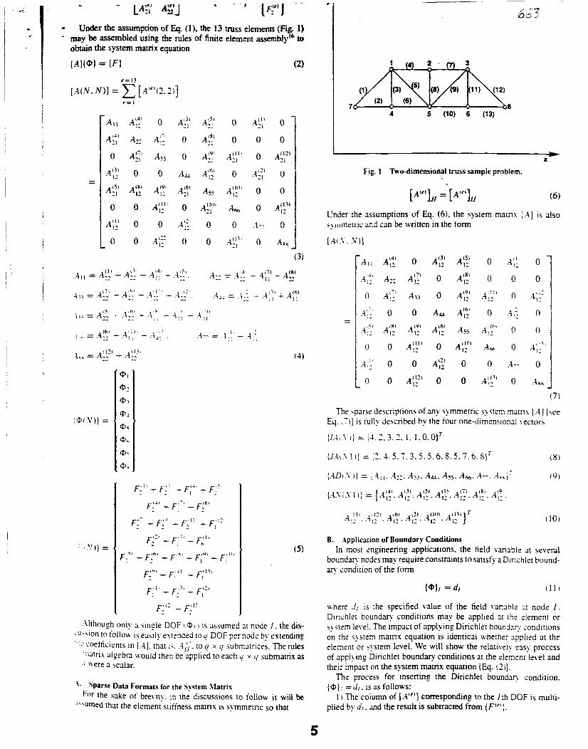
Figure 1 is a twodimensional truss (or rod) structure assembled from individual truss elements labeled (1). (2), . . . , (13) that are interconnected at eight nodes labeled 1.2. . . . ,8. An elemen: ) of the structure is assumed to possess only two points of connection- and the external loads are assumed to be applied at the nodes of the mss elements. Only a single de-- of freedom (Don at each node is assumed. To further simDlifv discussions. it is assumed that. by a

2nd RAhl for their assembly and soiution. This excessive CPC time 4 separate calculation. the eiemint stiffness mamx and external load and comuuter storage restrics aircraft noise predictior. codes to

! vector for the truss element ( e ) are known and expressed as ~~ ~

Uhough onl? ,I \ingle DOF \ @, I is assumed 21 node I . the dis- . w o n to tollou I \ ejcil) evrsnded to u DOF per noas b> extending

2 Loetticients in I 41. that I \ 4,'' .IO q x q suom~rnces. The rules q bubmatnx as mtrix algebra iiould then oe applied to each y

t liere a bcalar

L Sparse Dau Formats for the Jvstem Matris

.:\\umed that the element stiffness matrix IS sgmmetnc so that For the sake of brevity. 13 rne discussions to follow it will be

1 * X

Fig. 1 -0-dimensional truss sample problem.

[A"'L, = [A'"],, (6)

Under the assumptions of Eq. (6). the system mami [ .4 I is also

The \parse descriptions of any symmetric system m m x I ,-I ] [\re is tully described by the four one-dimensional vectors Eq.

Ill A I ? . (10)

B. appiicatron of Boundar! Conditions In most engineenng applwtons . the field \msbi;: at several

bounds? noaes may require constraints 10 satist! a Dincniet bound- L. condition of the form

\\nerc J, is the specified value of the field \.anaSlc 21 node 1. Dinciiier boundan. conditions may be applied 21 thr Aernent or system Ievei. The impact of applying Dirichlet b o u x d q conditions on the system matnx equation is identicai ivhetne: sppiied at the clement or cystem level. We will show the relativeiy tasy process of applying Dirichlet boundary conditions at the slement level and their impact on the system matrix equation [Eq. t2J].

The process for inserting the Dirichlet b o u n a q condition. { @ I ; =d,. is 3s follows:

1 '\ The coiumn of corresponding 10 the I rh DOF is multi- plied by d,. md the result is subtracted from ( Ftr1) .

5

~~~~~ ~ -

2) The column corresponding to the I th DOF in [A("] is made

-. 3) The row corresponding to the I th DOF in [A("] is made zero. 4) The modified element matrix and the modified element load

5) [A]// IS made equal to unity. and { F], is made equal to J,. Thus. applying Dinchlet boundan. conditions to the system ma-

zero. . vector are assembled.

m\ equation modifies Eq. ( 2 ) to

[,i](@l = {PI (121

r - !JC( 1 1 1 ) = 17.7. 1.7.4.4.1.7.5.5.5.3.3.5.5.6.6.6.S. S.8)'

and the follou ins integer matrix:

1 0 0 0 0 0 1 0 1 1 1 ) 0 0 0 1 0 0 1 0

1 0 0 1 0 0 0 0 1 1 0 0 0 0 0 0 1 0 0 0 1 0 0 0 0 0 0 1 1 0 0 0

[€ ( .M. .S l ]= 0 1 1 0 0 0 0 0 0 1 0 0 I O 0 0 0 0 I O 1 0 0 0 0 0 0 0 1 1 0 0 0 0 1 0 0 1 0 0 0 0 1 0 0 0 0 1

- 2 3 6 7

13 15 IS 19 0 1 5 1 1 0 0 I O 16 0 0 0

1 0 0 0 0 2 0 0 0 0 0

(15) [ H.4 .I.. .LIZ I ] =

The t ~ v o one-dimensional integer vectors in Eqs. (13, and (141 are h 0 0 0 0 0 1 0 1 -

d x [ A ] *ill have rhese nonzero tcnns. The exact locatiom tmH & column numbers I of those three nonzero terms in [ A ] be Eferred to as 6164

( I R R J A = 4. (JC)a = 7. {IRJ = 4

(JQ = 4. (IRJI; =4. (JCJ11 = 5 ( 1 ,

122:

Thus. the three nonzzm terms of the founh row of [ A ] are located ;il row 4. column 7 : rou L. column 1: and row1. column 5 . respecti\+ iue Es. U)I. . -

The num_erical values of the coefficients in the modified c!s~em main\ 1.41 remain unchanged from those in ( A ] . elcept for 3 feu ;ha; are mads zero during the application of the Dirichlet b o u n d q conditions. Therefore. ue will illustrate application of the assembly 31gorithms to the nonzero pattern of [A ] .

The integer m a t m ;HA] and system matrix [ A ] can be altema. lively stored as one-limensional vectors:

{ho( . t f ) ] = f2.3.6. -. 9.8. 12. 11. 13. 15. 18. 19.

4.5. 1 1 . IO. IO. 1'. 31. 1.20)' (1'

C. Sparse Assembly Algorithms Three symmetric sparse assembly algorithms will be expiained

i n rhi\ section. The purpose of Fach assembly algorithm IS to fen- sratc the system loads vector { f . } and the four vectors denned ny Eqz. ! & I O ) . which correspond to [ A ] . The assembly algonrhms arc dixcused \ianing u i th the simplest and proceeding to the most complex.

The main ideas of a!gc.rithm 2 can be wmmarized by the follo\ving compurationsl tasks:

I ) After initialinns ihu} IO a zero vector. process all elements ( i n

ascending order) IO ?Stain the integer vector< ( I R } and { J C ) ~ h i k assembling 1.41 into !J].

2 ) Separatc the di2;onaI an3 nonzero off-diagonal temis of 14 from [ ( I ! and store th:. information in (AD1 and {AV} . Separate ti-. diagonal and off-diagcnal temis in I /R) and (JC} . and compute V.4 and (!A].

where

I

(rig. i ). 1 ne concep or an elemenr-uur matrix is easily exrended to q DOF per node by extending tafh of the unity coefficients in [ E ] to a q x q identity mapix.

* To minimize &e RAM, it is Comrenimt to descr ik rhe element- DOF matrix [ E ] by the two one-dimensional vectors

(IE(NE + I )} = [ l . 3.5.7.9. 11, 13. 15, 17, 19,21.23.25.27)'

a.

: = I

(23) (JEO\'€ x N P ) ) = 17. 1.7.4.4. 1. 1.2. I . 5,

45.2.3.5.2.5.3.5.6.6.3.3.8.6.S)' (21)

m d the transpose of the element-DOF matrix ( [ € I r ) by the follow- ing two one-dimensional vectors:

(fn(.l' A 1)) = { I . 5 . 8 . 12. 15.20.23.25. 27' ( 2 5 )

!JET(,\€ x N P I ! = { I . 3 .4 .5 .4 .7 .8 ,? ,9 . !!. ! ? . 2 . ? .

6 . 5 . 6 , s . 9. 10. 10. 1 I . 13. 1.7. 12. 13)' (261

The main ideas of algorithm 3 can be summarized by the followin:

!! .ksume :hs: ! / E ; . {I&;. [;ETi, aid {YrT?) have aiready been computationai tasks:

detined from the connectivity information (see Fig. 11. a) Compute (IC) and (J.4) (symbolic ssembly phase I .

b ) Cornpure ( / A ) from Eq. (30). 2 ) Assume [hat vectors ( I A ) and [JA) have alread!. been derined

from rhe symbolic 3ssembl> (task 1 ).Compute (.4,V) and {.4Dj from [ ; \ ' I I ] ~numencal assembl! phase I.

111. Sparse Algorithms for Solving Spmetrical Equations

In this section. the major tasks involved in solving \pane \ys- :i.m\ of linear equations are brietly explained. The S U C C ~ S ~ ~t ihe \parst' bolver i > due 10 improved technologies (Le.. equation re- ordering. matrix decornpo4on. superncdes and ICWP unrolling. ior- \vard:hadiward wlurion phases ) and bookkeeping strategieS ideal for implementation on 3 digital computer. More drtailud information on improved technologir.3 can be obtained from Refs. 2-11.

[ A ( . \ . .Y)] =

,A. Sparse Reordering Algorithms .After !mpo\ing the boundary condition\. rhe moditied stirini.ss

m t r i \ [ .4 I can be obtaincd from 1 A I as indicated in the di\cus\ions .-tore Eq. 12). Equation ( 121 \hould iievcir be \olved directl!. To runher xirnpiify rhe Ji lcuswns. we will aswmr. that mairix .i; 113 rhr tollowing numericlri values:

- l o 6 6 0 0 0 0 2 O I I l O

1271

1 5 0 0 1 8 8 0 3 o o o o u 1

Thw. in this case 3' = 6 3nd .V 1 = 6. During the factorizarion phase. man! of the zero-value terms appearing in Eq. (27) ma! become nonzero. For masimum efficiency of storage and solution time. rhr equarions are reordered so that the number of nonzero terms thst occur during factorization are minimged. These extra nonzero terms Crclrted during the tacronzarion of [ A ] are referred to as till ins 3nd are denoted by the symbols F in the folloumg equation:

1 X X X 0 X . Y X F X F F

ln kq. (B,, o n e m eight exna (or new] noms0 nR m. As a result,

N F = 8 Do- (29) f -c

N2= N l + N F = 6 + 8 = 14 (30)

In general, the number of nonzero coefficients in the upper triangular pan of [ .1] after factorization ( N 2 ) is much larger than those before factonzation ( N 11.

The purpose of reordennp algonrhms [multiple minimum degrees (MND), nested dissection. or AIETIS algonthms] IS to rearrmge the nonzero terms of [A] . defined m Eq. (17). to different locnions so rhat .V2 is minimized_' '*-" For example. applLing the fI3ID reoroenng algonthm to [ A ] s i l l result in the foIlo\ring permutarion and inverse permutation \ ecrors:

{fP(.V)) = (5.6.3. 1.4. 2 ) r . (A'OV)) = (1.6.3.5. 1. 2 ) r

( 3 ; I

With the permutation am! ;/P}. the m a t m [A] in Eq. (?? t can be transtormed into

1 " 44 0 0 3 0 1

(321 I 0 0 8 8 5 0 0 0 6 6 0 1

[ i R ( ' V . .\',I =

0 3 1 5 110 7 ' 0 0 0 7 112

\ON. if one tactorizes 1 i,]. there \ % i l l be onl! one t i l l 111 rhdt occurs. J) tollw \:

1 s 0 0 x 0 f s 0 0 .Y 0

1 1 s .Y s

R. Sparse S?rnhoiir Fartyization

one-dimensional vectors: The reordered matns [ .-\R j can bs described b! [he td lou i n s tour

( / A ( ' % - I I) = { I . -3.4.5.6.7.7)'

{JA(.\'II~ = {4 .6 . j . 5 .5 .6} ' (3-11

( A D ( i Y ) ) = j 11. 44.66. 88. I 10. 1121'

(Ahr(JYlil = ( l .2 .3 .1 .5 .7 lT (351

In rhis example. .V = 6 and .Y 1 = 6. Before performing rhe numer- ical factorization. it is necessary IO go through thc. sparse \!mbolic factorization. so that the tollou kng hold true:

1) The nonzero pattern of [ .4RF] can be determined iincluding the locations of till ins I .

2 ) The value of N ? can be determined so that adequarr com- puter memory can be allocared for the subsequent sparse numerical facrorization phase. On completion of !he sparse symbolic iactonzarion phase. the

nonzero patterns of [ .4RFj x e completely k_no\vn. and the moditied vcrsion j of Eqs. (31) and I 35 J for the tacrored marnx . ~ K F j <an he computed as

{/AriV- 1 1 1 = ( l . 3 . 1 . 5 . 7 . 8 . ~ ) '

(JA(A'2) ) = !1. 6.5. 5.5.6. 6IT (361

In rhis case.

N ? = l ' I - : \ F = 6 + 1 = 7 (371

Efficient sparse symbolic factorization algorithms and detailed FORTRr\N coding can be round el~ewhere.-.~-'

C. FindingSupnaodrs To understand the concept of a supemode tor master node). notice

that. in q. (33). 2-3 and 4-5 have the same nonzero panerns. That is. the nonzero terms in rows 2-3 correspond to the same column numbers. Equation (33) can be used IO define a master DOF vector

(!kf5Sc A')} = { 1.3.0.:. 0. 1 y (38)

?e master DOF t ector (MS} is based on the assumed system matnh [ A R ~ ] defined in Eq I 33). Once Eq. (35 I has been defined. effective loop-unrolling techniques' 23 can be used to improve computational speed dunng the sparse numencal factonzation phase.

D. Sparse Sumerical Factorization Phase The strategies employed in this phase are quite similar to the ones

used during the sparse symbolic factonzation phase and have been well documented in the Tne reordered system matrix ! 1 can be decomposed or factorized as

l & l = 14[c:4T (39 1

Here. ID] I C a diagonal and [ L ] i \ unit iower triangular matril. and

I ( 1 = 1. .I = 2 . . . . . .I' )

1 1 1 I

E. The \ (hi ion IU the \!stem matrix e;a3t:or, [Eq. ! I ? ) ] i \ obtained

in thret. phases: I ) in thr. nrst phase ifonrard so1u:ion phase). an intermediate

solution vector (@FF) is computed t r m the solution ofthe matrix equation

Solution IO the S!*tem Zlatrix Equation

[ L l l @ F F l = : F R I (42)

2 ) In the second phase (backward soiurion phase). a vector (@BE) is computed from the matnx equation

[~l[flr(@BBl = 1 @ F F l (43 )

3) ln the thirdphase(backrransformxionphasel.thevector ( @ B B ) is transfomed back to the original unkfi0u.n vector [ @ ] by utilizing the inverse permutation vector IN}.

IV. Three-Dimensional Aeroacoustics Application The de\eloped a1,oorithm will be exercised to study the propa-

p i o n otacoustic pressure waves in 3 :nree-dimensional duct lined with sound absorbing marerials (acoust;; iiners, as depicted in Fig. 2. The duct is spanned by axial coordinare :. transverse coordinate .I-.

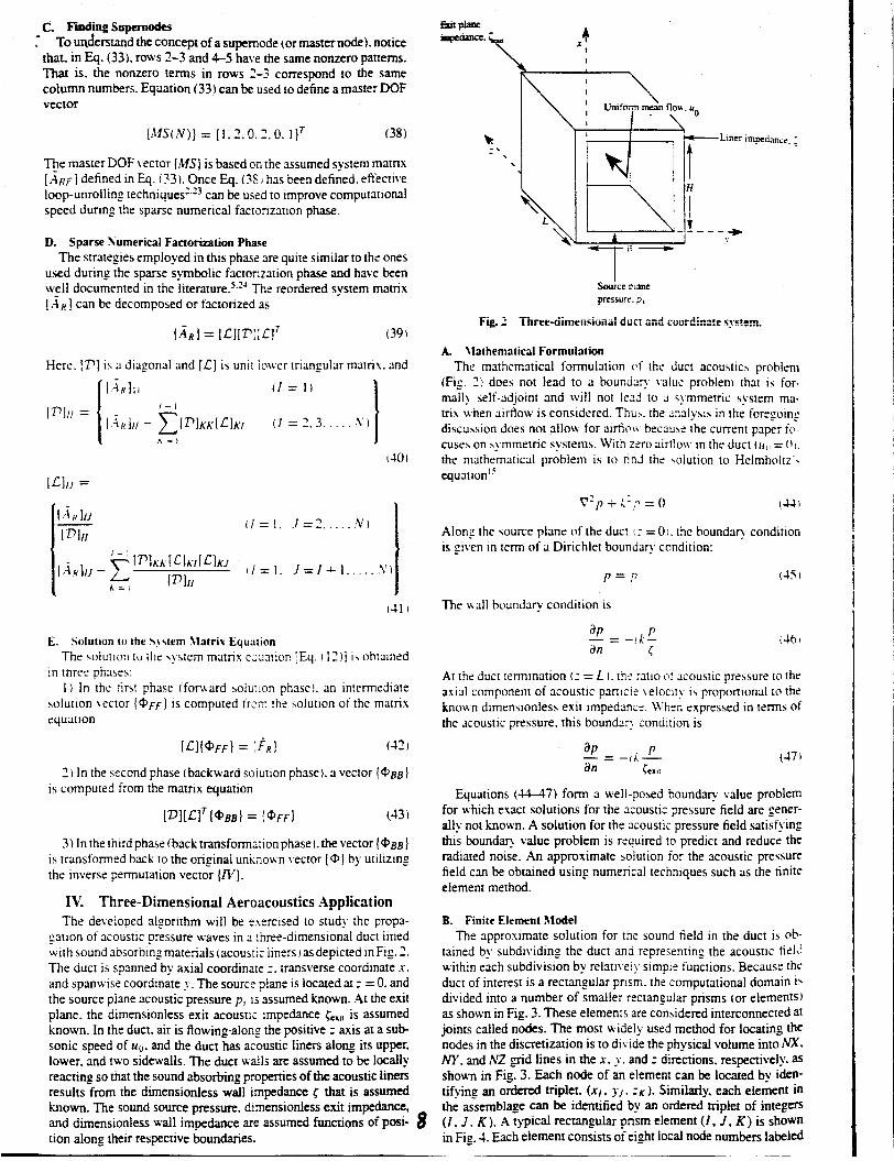
and spanuise coordinate y. The source plane is located at 1 = 0. and the source plane acoustic pressure pI is assumed known. At the exit plane. the dimensionless exit acoustic impedance (;lll is assumed known. In the duct. air is flowing-along the positive z axis at a sub- sonic speed of uo. and the duct has acoustic liners along its upper, lower. and two sidewalls. The duct walls are assumed to be locally reacting so that the sound absorbing propwries of the acoustic liners results from the dimensionless wall impedance < that is assumed known. The sound source pressure. dimensionless exit impedance, and dimensionless wall impedance are assumed functions of p s i - 8 tion along their respective boundaries.

pressure. 7.

Fig. 2 Tinrw-ciimeiinio~aii7li: dix: 2nd cc;crdins!e rystem.

A. \lathematical Formulation The mathematical formulalion c ~ f the duct acoustics probleni

(Fig. 2.1 does not lead to a bounuay value problem that i h for- mall! >elf-adjoint and will not Itad to a zymmetric system ma- t r ix when airflow is considered. Thw. the malysis in the foregoing discussion does not allo\v for airfiou becau>e the current paper fo- cuses on symmetric systems. With zero airflon in the duct ( i l p , = 0 I the niathematical problem is to rind ths solution to Helmholrz'. equation I'

T2p t L::7 = 0 (41

Along the hource plane of the duct I: =OI. the hounda? condition is given in term of a Dirichlet boundary condition:

p = p , (45 I

The \\.all boundav condition is

At the duct termination (: = L 1. t k i3110 cf acoustic pressure IO the axial component of acoustic panici: ielocity is proponional to the knobvn dimensionless exit impedance. IVhen expressed in term5 of the acoustic pressure. this bounds? rondition is

(17,

Equations (5.117) form a wel!-posed boundary value problem for which exact solutions for the a:oustic pressure field are = Oener- ally not linown. A solution for the acoustic pressure field satisfying this boundan value problem is required to predict and reduce the radiated noise. An approximate solution for the acoustic pressure field can be obtained using nurnencal techniques such as the finite element method.

B. Finite Element hlodel The approximate solution for t h t sound field in the duct is ob-

tained by subdividing the duct and representing the acoustic tiel~: within each subdivision by relativti)- simpie functions. Because the duct of interest is a rectangular prism. the computational domain is divided into a number of smaller rectangular prisms (or elements) as shown in Fig. 3. These elements are considered interconnected at joints called nodes. The most widely used method for locating the nodes in the discretization is to divide the physical volume into m. M . and hZ grid lines in the s. J. and z directions. respectively. as s h o w in Fig. 3. Each node of an element can be located by iden- tifyins an ordered triplet. (XI, JJ. z ~ ) . Similarly, each element in the assemblage can be identified by an ordered triplet of integers (I, J. K). A typical rectangular prim element ( I . J . K) is shown in Fig. 4. Each element consists of eight local node numbers labeled

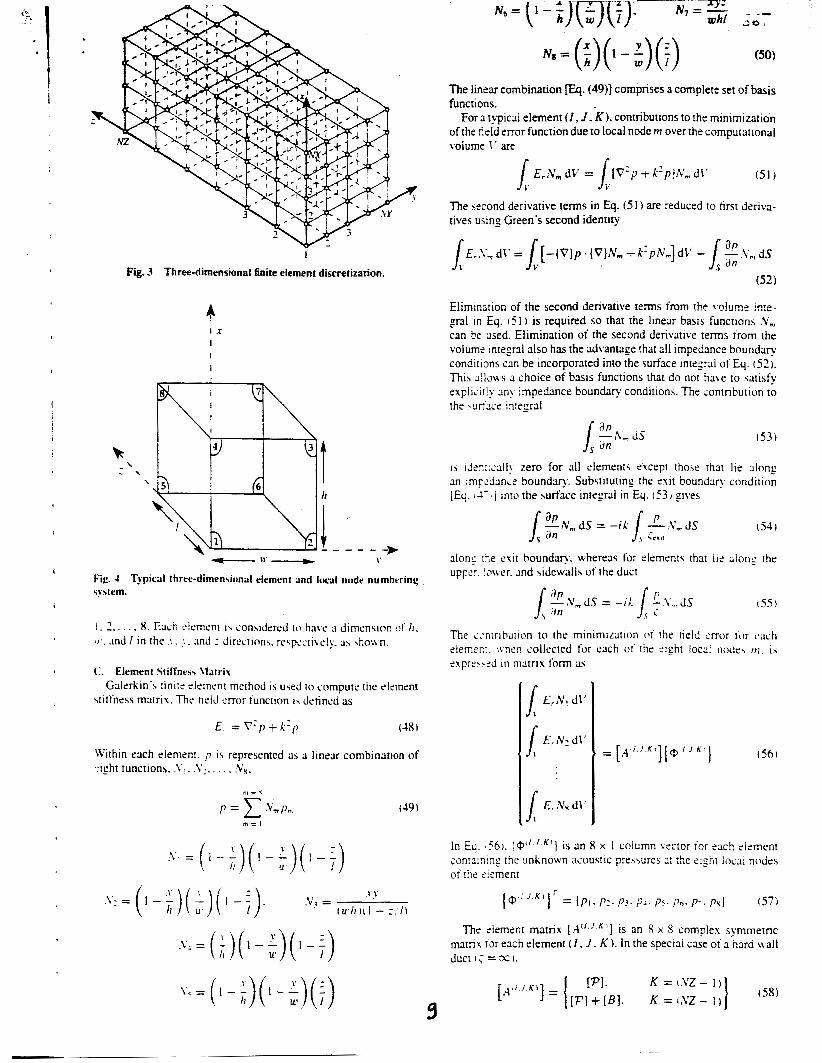
1

Fig. 3 Three-dimensional finite element discretization.

? I I I I I

)r \

- \ \

I

Fig. 4 \!mm.

Typical thret.-dimen\ionaI clement and local ride numbering

, i. 2 . . . . . 8. Each i'kment I \ conudercd to have a dinien4ion ef I!. w . and I in the l. .. . and : dirsctions. re>p:L$\rly. 35 \ho\\n.

( C. Element Stifhe\\ \!atri\ Galtrkin.\ tinirs clement method i s used to compute the rlrment

stiffness matrix. The tleld error function 1 4 detined as

(48) E , = '?:,I i- k ' p

Wthin tach element. p 15 represented as a linear combination of .:ight functions. .\:. .Y:. . . . . .Yy.

(49)

9

The linear combination [Es. (49)] comprises a complete set of basis functions.

Fora typical element (I, J . K ) , contributions to the minimization of the rield error function due to local nodem overthe computational volume I ' are 1 E,;\', dC' = l [ V 2 p + k ' p ] N , d l ' (51 j

The second derivative terms in Eq. (51 are reduced to tirst deriva- tives using Green's second identity

(52)

Elimination of the second derivative terms from the \c!u-e :ng- g a l in Eq. ( 5 1 is required so that rhe linear basis functions ,V,, can be used. Elimination of the second derivative terms from the volums inteprsl also has the advantage that all impedance boundar?, conditions can be incorporated into the surface integral of Eq. 152). Thi:, d lous a choice of basis functions that do nor have to satisfy explic:ily an! impedance boundary conditions. The ~onrribution to the \uc'3ce Integral

(53)

I\ i j e x a l l ! zero for all dements swept thow that lie dong 3n imr:Jinie boundary. Substituting the r ~ i f boundar! condition [Eq ,4-1 j into the wrfacr integral in Eq. 1531 gives

alon; :he ryi: houndac. whereas for elements that lis ~ilong the uppsr. !oucr. and sidewalls of the duct

The ;.mrritrutlon to the minimization of the rield m o r ior each tlemx:. ,.\hen collected lor each o t the right loc~il node\ ! T I . is exprr\*td in matrix. form as

l E, N , d1'

E, IV: J1' l E,iVxdl'

(5.61

In Eq. 261. I@" is an 8 x I column \ m o r for each element ionrainmg the unknown acous!ic pre5su:es 2: :hc eighr 1oc;Li nodes of the tisment

{ @ ' . K ' ] ' = { P I . P:. p ? . p;. p ! . p,. p - . p ? ~ 7

( 5 7 )

~ h c s~emenr marrix [A{' . ' .~ ' ] is an 8 x S complex symmetric matrix tor each element ( I . J. K ) . In the special case o f 3 hard \vail

Here. [F] represents the contribution to due 10 the element volume 1'. uhereas ( B ) represents the contributions due IO the exit plane b o u n d a ~ . The matrices ['PI and [ B ] are symmetric. and their coefticients h a c been computed explicitly:

1

2 1 2 8 4 2 1 x 2 2 2 x 1 - 1 4

L 2

-1 - I

I 3 -

1 4

-1 7 - -

IhOl

thl I

1 1: - 1 ' 2 I -2 -1 -2 - 1 - - 1 2 -4 -2 - I -2

j ' 1 2 - 1 -2 -1 - 2

1621

1631

V. Results and Discussion Th- ihrri.-Jimensional rigid irall acou\tic elenicnt ha.; been cou-

plcd u i t h thc sparsc asscmbl! and rquarion \olier dgorirhms to pro\ idc a w n i h l y and solver statistics for a threc-Jimtn5ional duct xrodioustic4 application. Computations presented in this paper u t x run on 3 singlc processor tvith double-prccihn cN-biti xith- mtiii on ai1 ORIGIN 2oOO computer platform. The \parse equation \ t i l \ rr II\CL! \1I lD rrordering. Computation\ a:? pre5ented for :: unitomi ;rid and a geometry identical to that o i the Lanyle! Flou Impd;incc Tubc. Thi\ three-dimensional duct has H square cross \c'ciic'n 0.050S m in u idth (I\. = H = 0.05OS rn ; and 0.8 12 m in lrn:tli tL =O.S12 mi. A more detailed descripiion of ths duct is y e n in Re!. 15. All calculation6 were performed at standard at- rnmpheric anditions without flou. and the source frequenc! was c h w n to >pan the full range of frequencies currenil! of interest in duct liner mearch. The sound \vas chosen as a plane nave ( p > = 1 1. and thr dimen5ionless exit impedance \\'as chosen 33 unity i<c\lt = I I. Thi4 exit impedance will simulate a nonreflecting terminarion for the plane uave source.

Table I presents CPU statistics tin seconds, for each of the three awmbly algorithms and the sparse equation solver a5 a function of the hource trequency f. in kilohertz. The CPC rime for the solver ccolumn 9 I i s that required to obtain the solution \ ector after the sys- tem matnx was assembled. Note that before obuininy the solution vector. the \!stem matrices obtained from each sssembly algorithm \\ere compared to each other. Each asembly algorithm assembled the idsnrical \!'stem matrix as expected. Also included in Table 1 are ths number of :rid lines NX. .A?'. and A'Z and the matns order .\ Ih31 \vert used tf i perform the computations at each irequency. Here ha\? used the generally accepted rule that 12 poinrs per \va\elength is rquired to resolve a cut-on mode in each coordinare direction. To establish the accuracy of the solver solutions. the relati\e error norm (Relerri. computed from the solver solution vector. \vas tabulated in the tinal coiumn of Table 1. The relative error norm: is defined as

IO where

{EN)' x {EN)T ( F ) = x { F ) T

Relerr = (66)

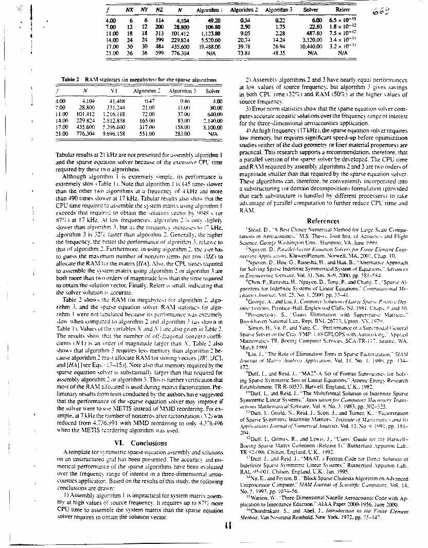
- ,' ' 3 W e 4 f NX M' N &omtun: Aigoxi&m2 A.lgmlnn3 Sober R e b

4.00 6 6 114 4,104 4920 OW 022 7-00 12 12 200 28.800 106.80 250 1.75

487.80 7.5 x IO-" 11.00 18 18 313 101.412 1.13.80 9.05 2-28 3.120.00 3.4 x IO-" 14.00 24 24 399 ~ 9 . 8 2 4 s.s20.60 20.74 14.24

17.00 30 30 184 435.600 19.488.00 39.78 26.94 lO.440.00 3.2 x IO-" 21.00 36 36 599 776.304 N/A 73.8 1 48.35 NM N/A

6Ml 6.5 x 22.80 1.8 x

Table 2 RAM statistics tin mepb!tesi fnr the sparse algorithms

f N .v I Algorithm 2 Algorithm 3 Solver

4.00 4.104 4l.46R 0.47 0.46 4 .OO 7.00 28.800 731.244 21.00 11.00 80.00 11.00 101.412 !.'16.118 72.00 37 .w 6.10.00 14.00 229.824 2.512.838 165.00 83.00 2.1-W.00 !7.00 435.6%? f.3'36.InX1 j i i . ( ? U 158.00 5.100.00 21.00 776.304 9.696.158 5 5 1 . 0 283.00 UIA

Tabular results af 21 kHz are not presented for assembly algorithm I and the sparse equation solver because of the exce\\i\e CPL' lime required by these trio algorithms.

Although algonrhm I is extremely \imple. its perfommce is extremely slon (Table I ). Note that algorithm I is I45 time\ slower than the other t u n algorithms at a frequency of 4 kHz and more than 490 times ilo\\er af 17 kHz. Tabular rewlrs alw shot\ that the CPU time required !o assemble the >!stem marri\ using alipithm 1 exceeds that required 10 obtain the \olurion iector b! l)olS \ (or 87'; ) at 17 kHz. .Ai low frequencies. dgorithrn 2 is onl! ,liptitl\ ,lo\ver [hail alpon!hrr! .3. bc! AS the :'itqiicnc! increa\cs IO i; kHz. algorithm 3 -32'; h t e r than algorithm 2. Generdl!. the higher the frequency. the better the performance of algorithm 3. rdatiie to that of algorithm 2 . Furthermore. in w i n g algorithm 2. tht u\cr ha\ IO guess the maximum number of nonzcro icm\ per rnu I \I21 to allocate the RAX1 tor !he matrix [/[.4 1. h h . thc CPC time\ rquired to assemble the \!\rem matrix using dgori thni 2 or algorithm 3 are both more than t\%o orders of magnitude le\\ than the time rtyuirLxj io obtain the solution \ector. Finally. Relsrr I \ \mall. indicating that the colver solution I \ accur;itc.

Table 2 she\\\ thi. RAM (in megabyte\t tor algorithm 2 . Ago- rirhm 3. and the \ p m e equation solver. R M l \talktic\ tor a l p - rithni 1 were not :abuIatcd hecause i t \ pertimi3ncc \.\a\ elitrcrnely \IOU when compmd 10 algorithm 2 and Jlgorithni 1 (as \ h w n in Table I 1. Value\ orthe variables A' and .Y I are also gi icn in TJbk 1. The results shou thai !he number o t ott-diagon;il nonzcro ioeffi- cients I N I 1 also \bows that algorithm i requires les\ memory than algorithm 1 be- cause algorithm 2 n u \ t allocate RAX1 tor 5torlng vectors {IRi. UC]. and [Ha-\] [see Eqs. 1 1-3-15)]. Note aI\o that memory required by the sparse equation \ol\sr is substantiall! larger than that required for assembly algorithm 2 or algorithm 3. Thi\ I \ tunher ieritication that most ofthe RAX1 Alomed is used during matrix factorization. Pre- liminary results trom tests conducted by the authors have sugyeaxJ that the performance of the sparse equation solver may improve if the .solver ivere to use 1IETIS instead of 3lblD reordering. For ex- ample. at 7 kHz the cumber of nonzero\ after tacrorization i V 2 I was reduced from J.X.39 I with MhlD reordering IO only 4.3-6.496 when the METIS reoidering algorithm uah used.

VI. Conclusions A template for Gymmetric sparse equation assembi!- and wlutions

on an unstructured 2nd has been presented. The accuracy and nu- merical pertbrmanc: of the sparse algorithms have been e\ aiuared over the frequent! range of interest In 3 three-dimensional 2eroa- coustics application. Based on the results ofthis study. the iolloiving conclusions are drau n:

I ) Assembly aigonrhm 1 is impractical for system matrix 3sxm- bly at high values or source frequent!.. It requires up to 8 7 5 more CPU time to assemble the system marrix than the sparse equation solver requires to obrain the solution vector.

an Ordrr of magnitude IJrgc'r than .\. Table

2 ) Xssembty algorithms 2 and 3 have nearly equal performances at IOU. values of source frequency. but algorithm 3 gii'es savings in both CPL lime (315) and RAM (50%) at the higher values of source frequency.

3) Error norm statistics show that the sparse equation +elver com- putes accurate acoustic solutions over the frequency range of interest for ihe chree-dimensionai aeroacoustics application.

4) At high frequency ( 17 kHz I. the sparse equation solver requires low memo?. but requires significant speed-up before optimizatrlon studies (either of the duct geometr)r or liner material properties) are practical. This research supports a recommendation. therefore. that a parallel version of rhe sparse sr?!ut.r he de:e!~pcd. =IC CP'i rime and R.4X.I required by assembly algorithms 2 and 3 are nvo orders of magnitude smaller than that required by the sparse equation solver. These algorithms can. therefore. be conveniently incorporated into a substructuring (or domain decomposition) formulation (provided that each substructure is handled by different processors1 to rake advantage of parallel computation to funher reduce CPL time and R X 1 .

r'Ashrraftt. c.. ~ompresstd ~r;tphs and the Minimum D C ~ AI- * eorithm.*; SIAM Joumul of Scienr~jc CompiiN'ng. %I. 16. NO. 6. 1995.

"Gamma. E.. Helm. R.. Johnson. R.. and Vlissides. J.."Desip Patterns: Elements of Reusable Object-Oriented Software:' Addison Icidey Prufes- sioriul C o n f p i m i , ~ Srrirs. Addison Kesley Longmm. Reading. MA. 1995.

"George. J . . and Liu. J.. "The Evoluiion of the hfinimum Degree Xi- goritnm:' SIX ire. .ior Itiu'itsrriai urd .+piid .Ilurhmioric.s. Vol. 3 1. No. 1. 198'). pp. 1-19,

'"Liu. J.. "Slodihcurion nf the Slinimuni-Degree Algorirhm h! Slulti- ple Eliminsrion.~' .hsoc iuiioii @w C O ~ J ~ ~ U I J J : . $fuc~h;t~rn. Trurisur-rrrm o ~ i

. W ~ r / i m u f i ~ d Sohi-crrc. Vol. I 1. So. 2 . I9Pi. pp. 141-53. -.I;um!en. G . . and Porhen. .A,. ".An Oh!ecr-Onenred Colleciion of 51in-

iniuiii Degree .Aiporithm\. D e ~ g n . Implemenrarion. and Experienceh-'

' pp. IJo*lIl.

pp. 12-30.

3 ,

NAS.1 CR-f999-20897 10%. ais0 Inst. for Computer ~ p p I i c p i ~ in sLi- 0'70 ence and Engineering. Rept. 99-1. h p t o n . VA. Jan. 1999.

':Amesroy. P.. Davis. T.. and Duff. I.. "An Approximate Xlinimum Degree Ordering Algorithm-- Compurer and lntomrarion Science Dep:.. TR-Y;-(i;ti. Unis. of Ronds. Gainesvine. FL. Dec. 1994.

2:fii3ryp~s. G.. and fiumsr. V.. "METIS: ljnstructured Graph Panirionln: and Sparse Xlams Ordminf.-' Ver. 2.0. Univ. of Minnesou. Xfinnespo~l,~ MN. 1995.

"Rune\ha. H.. and Nguyen. D.."Veciorized Sparse Uncymmetrical bud. tion Solser for Cornputnricml Slechmics-' imi~u/ic.es i r i E U L V J ~ C C U ~ I : j, :.. u'uI~'. VOI. 3 1. SO.*. LSY. ?MU. pp. 56.7-570.

P. J. \IOTTI\ . ~ s . s ( J ~ ~ ~ L u c ~ E c j i r o i .

prcipcrl\ Thc rc\r spends .i crrat deai (if'rilne scrrin; up a prohlcm heriire rlie Llni.in tilrcr I S a i r t i ~ l l y itirmul~rcd to ~ I I C the reader an intuiriw ice1 tilr the prc)hlem hcing ddrescd. k ~ i pri)hlcms .ire scl- doni prcsentcd in rhc form citdif- ierenrial cquxions md tiicy usually don'r haw uniquc wlurions.

Pnigrc>s i n . i w t i n ~ u r i c s .inL! .\en I I I J L I ~ I ~ S

2000. 670 pp. H.irdciivcr

List Price: $99.95 ruM Alembcr Price: S74.95

Sourcc. 945

ISRS 1-36347-435-7

Order 24 hours a oay at ww.aiaa.org

I2

I

3. Parallel Finite Element Domain Decomposition for Structural/ Acoustic Analysis: S_ymmetrical Case [Ref. 6.21

(Please refer to the attached Journal Paper for this section)

13

_ _ -

I

- PARALLEL FINITE ELEbIENT DOMAIN DECOkIPOSITION

FOR STRUCTURAL/ACOUSTIC ANALYSIS

Duc T. NCUYEE;. SIROJ TUNGKAHOTARA Department of Civil and Environmcntal Enginccring. 133 I<.-IUF Hall

Old Dominion University, Sorfolk. V-4 23529. USA dngaycnoodu.~du, toohtaah9yahoo. corn

WLLIE R. WATSON Computational Aidelling 6; Simulation Branch. 31s 126

NASA Langley Research Center. Harnpton. V.4 23661. USA u.r .uatsonQlarc . nasa.gov

Civil Engrneaing Depanmcnt. ECG 252 Arizona State Universic. Tcmpc. XZ S526T. USA

s.rajanQasu.edu

[Received: July 21. 20021

SUBRAMANIA~~ D. RAJAN

Abstract. A domain decomposition (DD) formulation for sol\-ing sparsc lincar systems of quaticas resulting from finite elcmenr analysis is prcscnted. Tnc iormulatioii incorporatcs mixed direct and iterative equation solving stratcgics and othcr n o d algorithmic i d m that are optimized to take advantage of sparsiry and csploit modern computcr architccturc. such as memory and parallel computing. The most timc consuming part of thc iormulation is identified and the critical roles of direct sparsc and iterative solvers ivithin tnc framcivork of tbc formulation arc discussed. Expcrimcnrs on smcral computcr platforms using rcal and complex test matrices are conductcd using sofm-arc basca on thc formulation. Sniall- scale structural examples are used to validate thc stcps in the formularion and largcscalc (l,OOO,ooO+ unknowns) duct acoustic examples arc uscd to c\aluarc thc parallel pcriormancc of the formulation. Results are presented using 64 SUN 10000. E SGI OFUGIS 2000 proccs sors, and a duster of 6 PCs (running undcr thc IVindoivs cnyironmcnt .. Statistics show that the formulation is efficient in both scqucntial and parallcl computing cnvironmcnta and :hat the formulation is significantly faster and consurncs lcss rncmor? tnan that bas4 on onc of thc best available commercialized parallel sparsc solvcrs.

hlathematzml Subject CIassificatzon: 74S05.15.W6. Keywords: linear dgcbra. sparse matrix computarion. parallcl cornpu~atioii. finitc cicnicnt. domain decomposition. strucwres. acoustics

1. Domain decomposition (DD) formulation for finite element analyses

Application of finite element -lysis to engineering probieins leads to the discrete equation system 11. 2)

Ircl(Zl= {SI * il.1)

- 190 D. T. Nguyen, ii: R. Watson. S. Tungkahotam onc: 5 Iiaian

where S, Z are vectors of length A' that contains the know: :.cia1 ioads and un- known nodal quantities. respectively. Here h' is a complex. s:c:;sni~ular. s\-nimet- ric/uqmmetric. KxIV sparse matrix. Although (1.1) assuiiies .? single loading con- dition (Le.. right hand side). multiple loadmg conditions mai be :reared by taking S and 2 as dense matrices, so that the j'h column of Z correspoiicc IO the A- unknown nodal quantities associated with the loadings in the j t h colunin c i s.

Using the domain decomposition concept, (1.1) is written I:: pnrritioned form

n-here submatrices KIB. I;s1, KII and I'BB have dimension zx:. nsm. mxm and nxn, respectively. The interior and boundary unknowns ji.e.. Z: and 2s) have di- mensions compatible nith the coiumns in KI1 and KBB: respec::\-eiy.

Eliminating the interior unknowns from (1.2) gives

K B z 3 = FB (1.3)

KB = KBB -f I<BI Q (1.4)

Q = -h;- , 'Kl~, (1 4 FB = SB + 0, (1.6) Q = - -h-BISI 1 (1.7) S I = h-&%l . (1.8)

where

Here ICB is the boundary stfiess matrix for the domain, F s is :kz v x t o r of boundary forces, and the superscript (i.e.: -1) denotes the matrix inverse Efficient sparse algorithm [3]-[ll] may be used to decompose sparse matris 1;:: x i solve for matrix Q in (1.5) and the vector 31 in (1.8).

In the current DD formulation 112, 131 the computational ao:::ai:: is decomposed into L subdomains and KB and f" are synthesized by cc::sik:n: contributions from all subdomains. For this purpose, t.he discrete equation s-,xc::: for a subdomain (n-hich is considered an isolated free-body) is expressed in rile 2::~. ,I.?;

....

I 1 ; i I ~

Finall,., KB and FB may be obtained espiicitly from the equations

(1.15)

(1.16)

where p) is a Boolean transformation matrix of dimension n("sn(+) .

The sequence of steps constituting the DD formulation proposed in this paper is ~ 85 f 0 U m .

(1) Decompose the large-scale finite element domain into L snider subdomains. Algorithms and software given in j12. 131 are used for this purpose.

(2) ComputeK$,Kgj,Kg), KgA. Sg'. and S:) using efficient sparse assembly algorithms [3, 111.

(3) Factorize the sparse matrix Kj;' and compute 3;'' using (1.16) and Q(') using (1.13). Algorithms and software for sparse symbolic and numerical factorization, loop unrolling techniques. equation reordering. and foru-ard- backward solution phases ([3]-[11: i are utilized at this srep.

(4) Compute Kg) and 3'') for each subdomain. (5) Compute K s and F3 from (1.17). (6) Solve (1.3) using a direct or iterative solver to obtain the boundary unknowns,

a): EfEcient parallel direct dense solvers given in [14:-!16! may be utilized at th is step provided that KB is formed esplicitly.

b): However, explicit computation of A-B is ai espe::sive operation due to the need to perform the inner produce Kg]Q(r' in ! 1.12).

c): Iterative solvers (such as the preconditioned conjugate gradient a lp- rithm) 1171 are therefore recommended for this srep in the formulation. The use of an iterative solver eiiminates the need TO form KB esplicitly because each stage of the iterative solution t?-pically requires only the product a matrix ( K B B +- K2;)Qr: x-ith a hoi\x vector.

(7) Finally, the solution for the interior unknowns are obtained from (1.11) by using the factorized sparse matrix I<:;' during the fonvard and backward substitution phases.

ZB-

The solution vectors obtained from the formuiation are post-processed to obtain other quantities of interest such as stresses. strains acoustic energ\- etc. The remainin, - sec- tions of this paper will'focus on issues relared to efiicient sparse assembly procedures.

16

192 D. T. higuyen. 11.. E. 1f;atson. S. Tungkahotara and S. D. Rnic:.

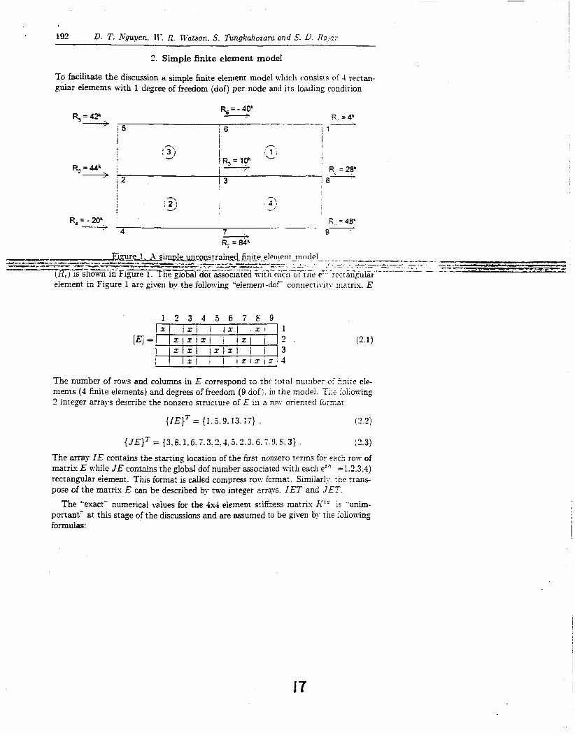
2. Simple finite element model

TO facilitate the discussion a simple finite element model which consists of -1 rectan- gular elements with 1 degree of freedom (dof) per node and its loading condition

izj R,=-20L , R =48'

" 4 7 9-

element in Figure 1 are given by the following "element-dof connecti\-ity inatris. E

1 2 3 4 5 6 7 6 9 1 2 . 3 1

(2.1)

The number of rows and columns in E correspond to the total number ci 5 i e ele- ments (4 finite elements) and degrees of freedom (9 dof). in the model Ti.? folion-ing 2 inreger arrays describe the nonzero structure of E i s a row oriented fo:niar

{ IEIT = (1.5.9.13.17) .

{JE}= = {3.8.1.6.7.3.2.1.5.2.3.6. i' 9.S.3)

12.2)

(2.3)

The array IE contains the starting location of the first nonzero terms for each row of matrix E while JE contains the global dofnumkr assoclared with each et" =1.2.3.4) rectan,dar element. This format is called compress roiy format. Similari:; :he trans- pose of the marrix E can be described by two integer arrays. IET and JET

The "exact" numerical \dues for the 4x4 element sTiEness matris K" is "unim- portant" at this stage of the discussions and are assumed to be given by the :b!ioning formulas:

i7

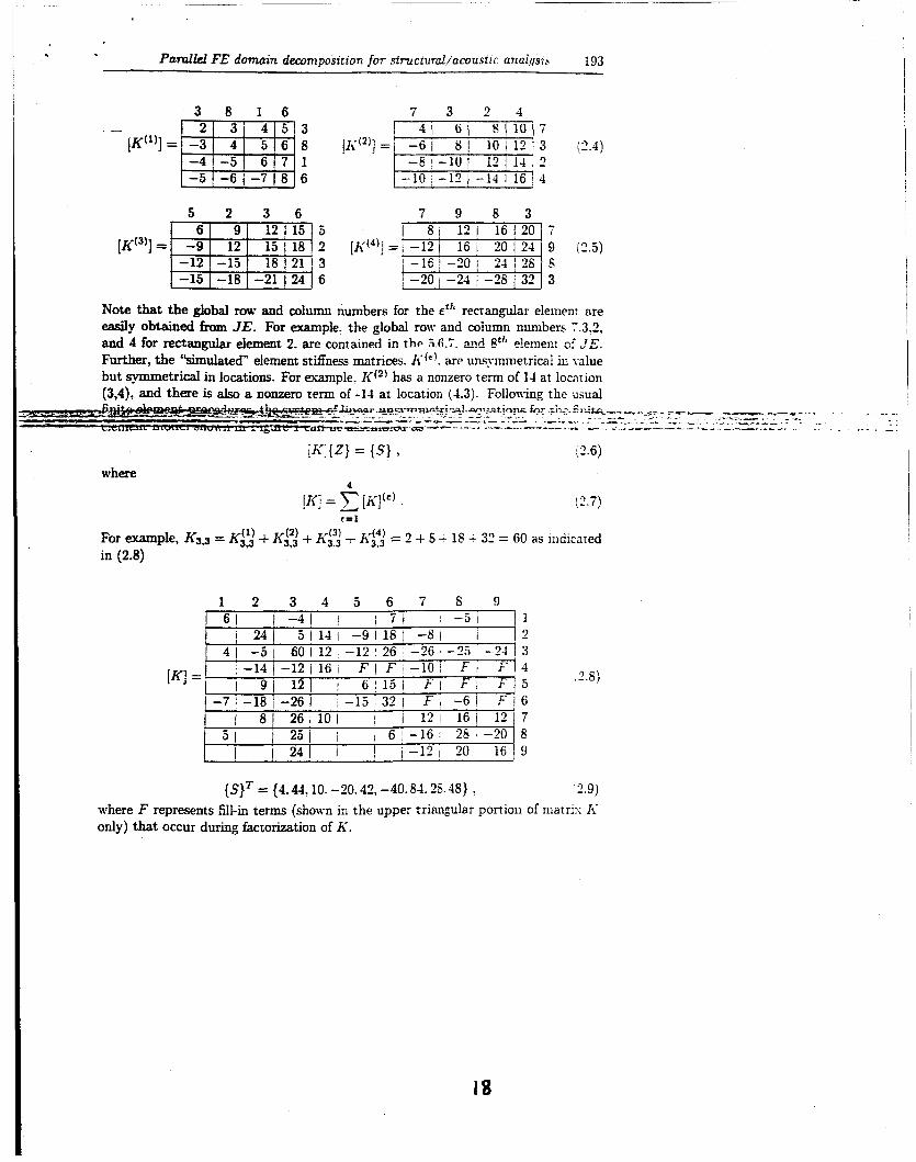
Parallel FE domain dewmposztzon for structuml/acoustlc analysis 193

- [K(')]=

3 8 1 6 7 3 2 3 2 ' 3 ' 4 5 3

-4 -5 6 7 1 - 5 1 - 6 1 - 7 1 8 6

-3 4 5 6~ 8 i 2.4)

2 3 6

[K"'] =

Note that the global row and column numbers for the E*)' rectangular eieinent are eady obtained from JE. For example. the global row and column numbers 7.3.2, and 4 for rectangular element 2. are contained in the 5 6 7 zr! Rt" e!emoz ci JE. Further, the "simulated" element stifiness matrices. h"'). are unsymnietrical i n ialue but symmetrical in locations. For example. K(*) has a nonzero term of 14 at locnrion (3,4), and there is also a nonzero term of -14 at location (1.3) Following the usual

L. - nTYLlc--cae - - - -.-ii ~ - - _ _ _ _ _ _ _ & - .

- - 4 - - . - c _ - - _ _ --. I-- I..-__- -.- -- - -

where 4

(2.7) e= 1

For example, K33 = K.f> + K f i + Kj3; - I<$ = 2 + 6 - 1P - 32 = GO as indicated in (2.8)

1 2 3 4 5 6 7 6 9 1 61 i -41 I ! 7 1 I -5 I 1 1 t - 8 I - 1

i 211 j l 1 - l i -91181 - 8 1 i 12 4 1 -5 1 60 I 1 2 -12 ' 26 -26 ' -25 -21 13

* - 1 4 / - 1 2 1 1 6 1 Fi F I - 1 0 ' F I F I 4 K] = ,2.S)

{S}= = (4 .4 .10 . -20.42. -40.61._3S.18} . '2.9) where F represents fill-in terms (shown in the upper triangular portion of mains Ii only) that occur during factorization of A'.

194 D. T. Nguyen. iI-. R. Watson, S. Tunoianotara and S. D Rqan

The solution to equation (2.6) is:

{Z}* = {l,l,l,l,l.l. 1.1.1) (2.10)

which has been independently confirmed by the results of the computer program developed. In the upper triangular portion of K . there are 9 fill-in terms. In order to minimize the number of fill-in t e r n during the symbolic and numerical factorization phases. reordering algorithms [lo, 131 sucb as muiriple minimum degree (MhID). Nested-dissection (ND), and METIS are used in the DD formulation.

3. Symbolic sparse assembly for symmetrical and unsymmetrical matrices

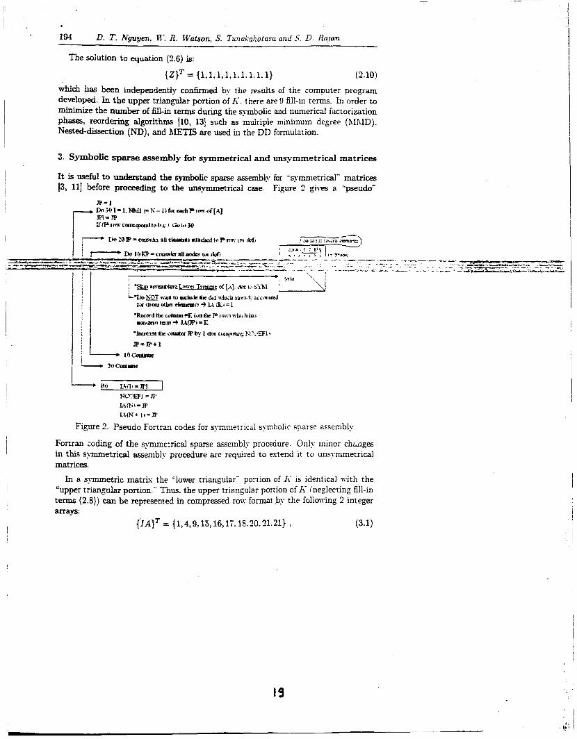
It is useful to undefitand the symbolic sparse assembly for "s?.rnmetrical" matrices 13, 111 before proceeding to the unsymmetrical case. Figure 2 gives a "pseudo'

- pa La:l,= If.1 1 NLu.sEF1 = w IArSi*]P I?W+ IJ=n

Figure 2. Pseudo Fortran codes for symmetrical s ~ n h l i c sparse assembly

Fortran d i n g of the symmcrical sparse assembly procedure Only minor chages in this spmetrical assembly procedure are required to extend I t to unsymmetrical matrices.

In a symmetric matrix the "lower triangular" portion of Ii is identical vith the "upper triangular portion." Thus. the upper triangular portion of I< (neglecting fill-in terms (2.8)) can be represented in compressed ran- format by the following 2 integer arrays:

{IA}' = { 1,4,9.15,16,17.1&.20.21.21} . (3.1)

j

i {JA}* = {3,6.S,3.~,5,6,7.1,3,6,7.8.9.7.6.6.6.9.9} . (3.2) I

Pamllel FE domain decomposition for structumljacoust~c analwrs 195 I

I where the array ZA contain the starting location of the first 11011-zero. ofi-diagonal term for each row of the upper triangular portion of K The difierence between any 2 consecutive integers on the right-hand-side of (3.1) will give the number of non-zero (off-diagonal) terms in a particular row of the upper triangular portion of K . For example, M(3)-IA(2) = 9-4 = 5. Hence, there are 5 non-zero terms (escluding the diagonal)) in row 2 of the upper triangular portion of matrix 1;. Additionally. J A contains the column numbers. associated with each non-zero. off-diagonal tern1 for each TOW of the upper trian,gular portion of matrix h-. Sore that 1.4 and J A arrays can also be obtained from the pseudo" Fortran coding shown in Figure 2.

The foliowing minor changes in the coding of Figure 2 are required to perform ~ ~ ~ ~ ~ ~ e t r i c a i assembly.

a): DO 30 I= 1, N (the last IOW will NOT be skipped) b): Introduce a new integer array L4IiEEP(N+l) tvhich plavs the role of array

LA(-), fcr sxmple: L%K€EF(I)= JPI . c): Remove the IF statement in Figure 2 that skips the lower triangular portion. As a consequence of this. the original array IA (-I will contain some additional. unwanted terms.

= - X d ) : ~ O u t p u t fmm - i ~ w n s y m n e i r i c Z sparse s i b b l y 11-2 be stored by LAKEEP(-) and JA(-). instead of IA(-) and JA(- as in the symmetrical case.

& I-- -.._ . - -- -- -

1. Applications

4.1. Software. The software that is based on the paralie: DD formulation presented in this paper has been developed. The parallel algorithm uses the message passing interface (h9PI) for interprocess communication and is therefore highly portable. The software developed is referred to as the direct iterative parallel sparse solver (DIPSS). DIPSS (in FORTRAN) incorporates a number of lower revel routines and provides o p tions for both real and complex matrices in double precision (i.e.. 6-tbir arithmetic). Itesults are presented for symmetric matrices only. \Ve use sparse factorization tech- niques presented in 131 and implement the preconditioned conjugate gradient iterative solver 1171 to solve the dense system (1.3). The following three esaniples are used to evaluate the proposed parallel DD formulation. Performance gains are particularly evident for large problems.

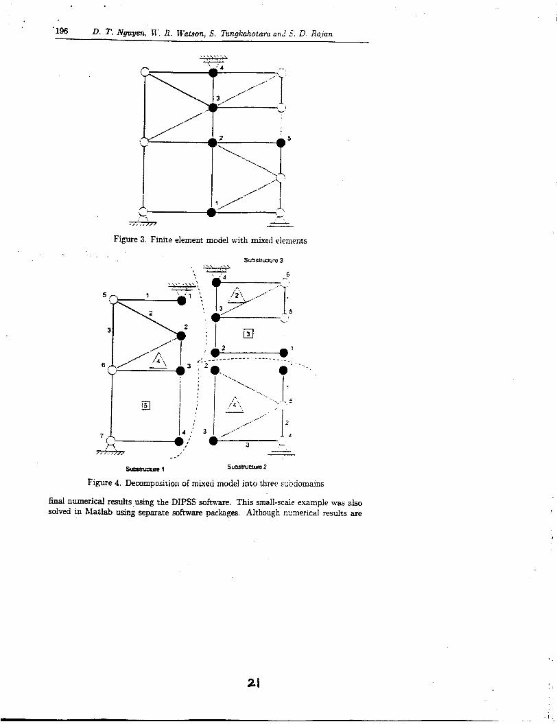
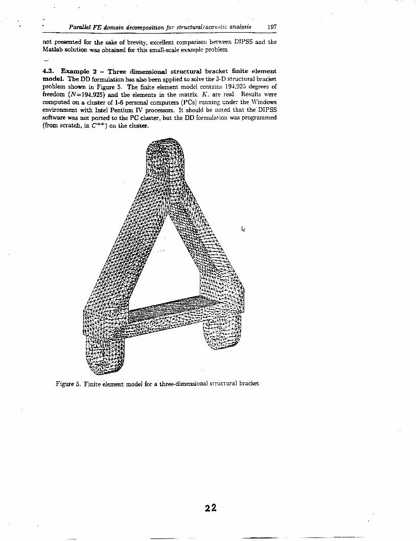
4.2. Example 1- Mixed finite element types. This is a srructural example for which the equation system is real and symmetric and has more rlian 1 finite element type. The entire finite element model is shown in Figure 3 and consists of ?-node "line' elements, %node Yriangular" elements. and &node "recr angular" elements. Interior and boundary nodes are denoted by open and filled circles. respectively. This small-scale. finite element model is decomposed into 3 subdoiliains as indicated in Fiewe 4. The prim- purpose of this exunple is to va!idate all intermediate and

20

'196 D. T. Nguyen, W. R. Ithtson, S. Tungkahotam and 5. D. X a p n

- -- sl&auaure 1 subslrucwre 2

Figure 4. Decomposition of mixed model into three scbdoniains

final numerical results using the DIPSS software. This small-scaie esample was also solved in Matlab using separate software packages. Although cnrnerical results are

21

Pm.dleI FE domain decomposition for structumQ'awust2c analysis 197

not presented for the sake of brevity, excellent comparison betwen DIPSS and the Matlab solution was obtained for this small-scale example problem.

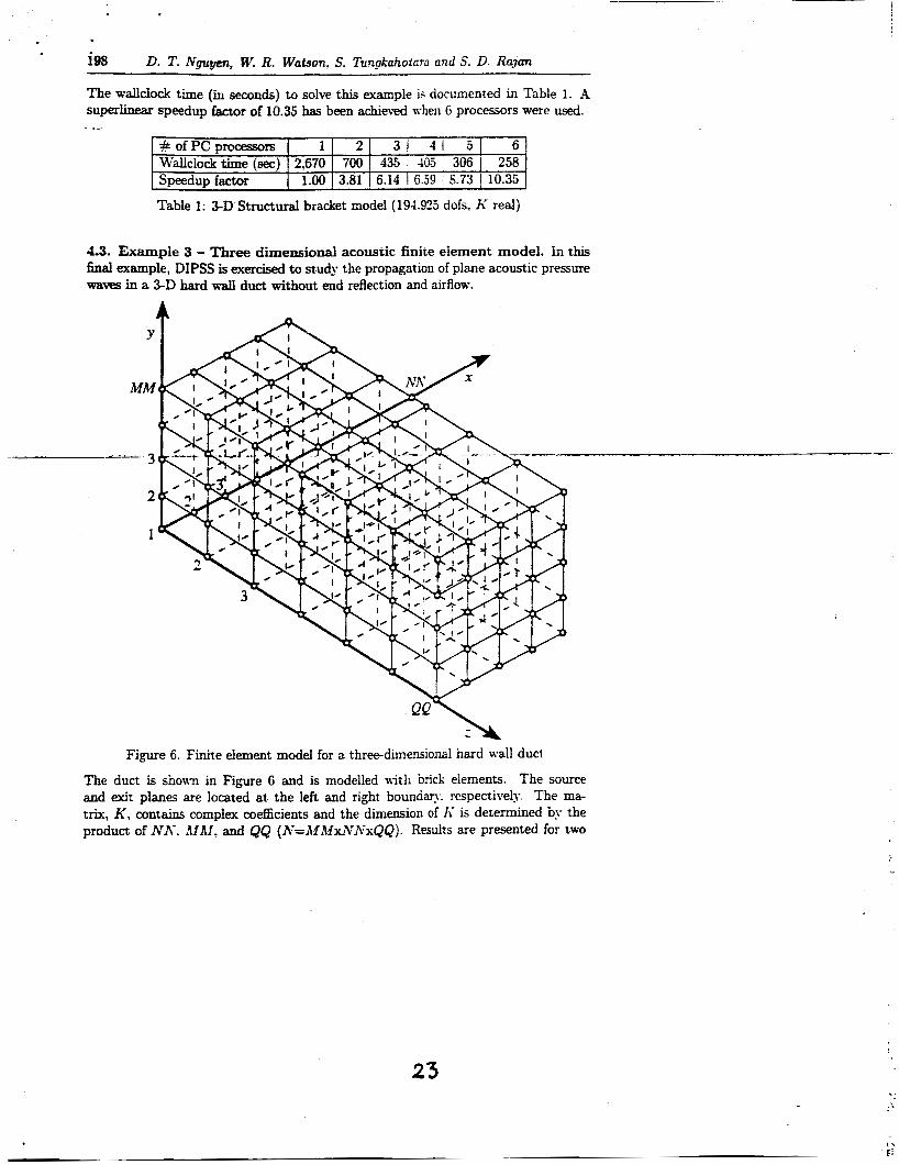
4.3. Example 2 - Three dimensional structural bracket finite element model. The DD formulation has &o been applied to solve the 3-D structural bracket problem shown in Figure 5. The finite element model contains 191.925 degrees of freedom (N=194925) and the elements in the matrix. K. are real Results were computed on a cluster of 1-6 pe r sod computers (PCs) running under the Wndows environment with Intel Pentium IV processors. It should be noted that the DIPSS software was not ported to the PC cluster, but the DD formulation was programmed (fro= scratch, in CUI on the duster.

Figure 5. Finite element model for a three-dimensional structural bracket

22

is8 D. T. Ngup, W. R. Watson, S. Tungkahotara and S. D. Rajan

The wallclock time (in seconds) to solve this e~ample is documented in Table 1. A suprhear speedup factor of 10.35 has been achieved n-hen 6 processors were used. - -

# of PC processors Wallclock time (sec) Speedup factor

1 1 2 31 4 1 5 6 2.670 1 700 435 1 105 306 258 1.00 1 3.81 6.14 1 6.59 I 6.73 10.35

Table 1: 3-D Structural bracket model (191.925 doh, A' real)

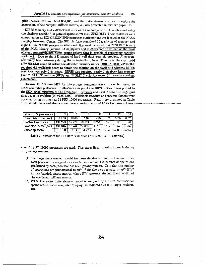
4.3. Exampie 3 - Three dimensional acoustic finite element model. in this final example, DPSS is exercised to study the propagation of plane acoustic pressure waves in a 3-D hard wall duct without end reflection and airflow.

Figure 6. Finite element model for a three-dimensional hard wall duct

The duct is shown in Figure 6 and is modelled with brick elements. The source and exit plans are located at the left and right boundary. respectively. The ma- trix, K , contains complex coefficients and the dimension of I< is determined by the product of NK. AIAI. and QQ (M=A4MxIVA7xQQ). Results are presented for two

23

P d l e l FE d a m decompsttwon for sttucturel/acoustrc analvusrs 199

grids (M=751,513 and A-=1.004,400) and the finite element analysis procedure for generation of the complex stiffness matrix, K , was presented hi another paper [lS]. - DIPSS memory and wallclock statistics were also compared IO those obtained using

the platform specific SGI parallel sparse solver (Le., ZPSLDLT). These statistics were computed on an SGI ORIGIN 2000 computer platform that was located at the XASA Langley Research h-. The SGI platform contained 10 gigabytes of memory and eight ORIGIN 2000 processors were used. It should be noted that ZPSLDLT is part of the SCSL library (version 1.4 or higher) and is considered to be one of the most efiicient commercialized direct sparse solvers that is capable of Derforming complex arithmetic. Due to the 3-D nature of hard wall duct example problem. h- encoun- ters many fill-in elements duurir?g the factorization phase. Thus. onl) the small grid (h'=751,513) could fit within the allocated memory on the ORIGIS 2OOO. ZPSLDLT required 6.5 wallclock hours to obtain the solution on the small ~d whereas DIPSS wallclock was only 2.44 hours. DIPSS also required nearly 1 gipabyte less memory than ZPSLDLT, and the DIPSS and ZPSLDLT solution vector (Z 1 were in escellent apreement.

Because DIPSS uses hlPI for interprocess communications. it cau be ported to other computer platforms. To illustrate this point the DIPSS softn-are was ported to the SUN loo00 DlatfOlm at Old Dominion Universitv and used to solve the large g i d duct acoustic problem (h' =1.001.400). Wallclock statistics and speedup factors were obtained using as many as 61 SUN 10000 processors. Results are presented ui Table 3 T t t e h a s u p e r l i n e a r speedup factor of SS.95 i w been achieve&- -- -----,--- --

Factor time (sec) 1 131.229 53.976 1 26.174 10.273 ' 3.260 909 1 56

n-hen 64 SUR' 10000 processors are used. This super-linear speedup factor is due to two primary reasons:

~

(1) The large finite element model has been divided inro 6-1 subdomains. Since each processor is assigned to a smaller subdomain. the mmber of operations performed tn, each processor has been greatly reduced Sote that the number of operations are proportional to ( T Z ' ' ) ) ~ for the dense nixris. or n('l.BiV' for the banded. sparse matrix. where B W represent the ha2 nand Kidth of the coefficient stifiness matrix.

(2) When the entire finite element model is analyzed by a direcr conventional sparse solver. more computer "paging" is required due to a larger problem S k

Wallclock time (sec) I 131.846 61.744 127.897 Speedup factor I 1.00 I 2.14 I 4.73

24

11.751 ! 3517 1.967 1 1.534 1i.z : 34.54 I 67.03 j 85.93

e

'200 D. T. Nouvm. U'. R Watson. S. Tunakahotam and S. D. Raian

5. Conclusions

A domain decomposition (DD) formulation for solving sparse linear systems of &pations ha^ been p m d . The formulation incorporates lower lwei novel dgo- rithmic ideas such mixed direct,/iterative sparse solvers, equation reordering. loop unrolling, efficient sparse assembly. and foward/backward solution phases that are o p timized to take full advantage of sparsity and exploit modem computer architecture. hrIedium to large-scale examples considered in this paper show that the developed h P I parallel DD &e is eflicient in both sequential and parallel computing environ- ments. Statistics show that s o h based on the formulation is si@icantly more efficient than that based on one of the best available commercidized, parallel, direct sparse solver. Acknowledgement. The authors would likc to acknowlcdgc thc many helpful commcnts sugkested by the revienas of th is paper and the NASA Langley Research Ccntcr for pro- viding financial support.

1.

2. 3.

4.

5.

6.

-r I .

a.

9.

10.

11.

12.

REFERENCES DESAI, CHAND-NT S. and .-EL. JOHN F.: Introduction to the Finite Element Method, Van Nostrand Reinhold Company, New York, N.Y., 1972. BATHE. K. J.: Finite EIement Procedures, PrcnticeHall. Inc., 1996.

N G U " , D.T.: Pamllel-Vector Equation Solver For Finite Element Engineering .4ppii- cations, Kluwer Academic/Plenum Publishers, 2002. QIN, J., GRAY, JR., C .E.. hiu. C. and NGUYEN, D. T.: A patallel-vector equation S G k T j % r UILsymmdrz c mahccs on supenomputers. Computing Systcms in Enginccring,

NGIJYE" D. T.. Ru"A, H.. BELEGUNDU. A. D.. and CHANDRUPATW. T. R.: Inte- rior point method and indefintte sparse solver for linenr pmgmmming problems. Advances in Engineering Software, 29(3-6), (1998) 409-414. NG-, D.T., HOU, GENE, R c x ~ m , H. and BANGFEI. H.: Alternatire approach for soiving sparse indejkite symm&cal system of equations, Advances in Engineming Software, 31(89), (2ooo), 581-584. NG, E. and PEYTON, B.: Block sparse Choleski algorithm on advanced unzprocessor ann- puter, Society for Industrial and .4ppiied hlathcmatics Journal of Scientific Computing, 14, (1993), 1034-1056.

DUFF, 1. and REID, J.: MA27-4 set ofFortran Submutinesfor Soltang Sparsr Sprnef~+c Sets of Linear Equations, AERE Te&nical Rcport. R-10533. Hanvcll. England. 1982. DUFF, 1. and REID, J.: The multijmntai solution o j indefinite sparse symmetnc h e m systems, Association for Computing LIachincry Transactions hIathcmatical Sofmarc. 9,

GEORGE, A . and LIU, J.: Computer Soiution ofL,arge Sparse Positive De-finite Systems, Prentice-Hall, Inc., Englewood CEs. KJ. Chap. 5 6: Chap. 10. 1981.

PISSANETZKY, S.: Sparse Matti;c Tehnolqy. Acadcmic Press, Inc.? London. U.K., 1984. hfOAYYAD. hi. A. and N G ~ . D. T.: An algorithm for domain decomposition mfinite element analysis, Journal of Computers and Smrrures, 39(1-4), (1991), 27-290.

2(2/3), (1991), 1W-290.

(1983), 302-325.

25

I 13.

14.

15. ,

16.

I 17.

, 18.

founws, G. and KUMAR, V.: METIS: l i n m ~ d Graph Partitioning and Sparse M& old-, Version 2.0, Univen4~ of Xlinnesota, 1995. TUNGKAHOTARA, S., NGUYEU, D. T., WATSOX, U'. R. and RuNESHA, H. B.: Szmple mad pmpllel h e quaiton solwrs, Eiinth International Conference on Numeri- cal Methods a d Computational Mechanics, July 1919,2002, Univ. of hlisblc, hliskolc, H w w Y - ANDERSON, E., BAI, Z., BISCHOF, C.. BLACKFORD, L. S., and D m , J. W.: Lapack Usm' Guide (Software, Enairmrments and Took, 9), Society for Industrial 6: Applied Mathematics, ISBN: 08987144?&3rd pkg edition, 2000. BLACKFORD, L. S., -01, J., CLEARY, A.. D'AzEvEDO, E. and DmMEL, J. W.: Scala- pock Umzn~' Guide, Society for Industrial 6: Applied Mathcmatis; ISBN: 0598713978;

PAPAD-, M., Brrwruras, S. and K O T S O P ~ , A.: Pamllel Solution Tech- RiQL(WiRC0mpUWWd . Sirudwnl M&ntcs, B. H. V. Topping (Editor), Parallel and Distributed P i a for Computational bIechanics: Systems and Tools, pp. 180-206, 1999, Saxe-Coburg Publicaticms, Edinburgh. Scotland. -WATSON. M'. R: Thne-dimarsroRol ' RctansrJnt duct d e with application to impedance

Bk&cdr edition, 1997.

&&ion, AULA Journal, 40, (m), 217-226.

2 6

.

4. Parallel Finite Element Domain Decomposition [Refs. 6.6,6.8] for StructuraVAcoustic Analysis: Un-symmetrical Case

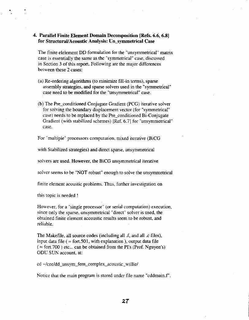
The finite elelement DD formulation for the "unsymmetrical" matrix case is essentially the same as the "symmetrical" case, discussed in Section 3 of this report. Following are the major differences between these 2 cases:

(a) Re-ordering algorithms (to minimize fill-in terms), sparse assembly strategies, and sparse solvers used in the "symmetrical" case need to be modified for the "unsjmmetrical" case.

(b) The Re-conditioned Conjugate Gradient (PCG) iterative solver for solving the boundary displacement vector (for "symmetrical" case) needs to be replaced by the Pre-conditioned Bi-Conjugate Gradient (with stabilized schemes) [Ref. 6.71 for "unsymmetrical" case.

For "multiple" processors computation. mixed iterative (BiCG

with Stabilized strategies) and direct sparse. unsymmetrical

solvers are used. However, the BiCG unsymmetrical iterative

solver seems to be "NOT robust" enough to solve the unsymmetrical

finite element acoustic problems. Thus. further investigation on

this topic is needed !

However, for a "single processor" (or serial computation) execution, since only the sparse, unsymmetrical "direct" solver is used, the obtained finite element accoustic results seem to be robust, and reliable.

The Makefile, all source codes (including all .f, and all .c files), input data file ( = fort.501, with explanation ), output data file ( = fort.700 etc ... can be obtained from the PI'S (Prof. Nguyen's) ODU SUN account, at:

cd -/cee/dd-unsym-fem-complex-acoustic-willie/

Notice that the main program is stored under file name "cddmain.f '.

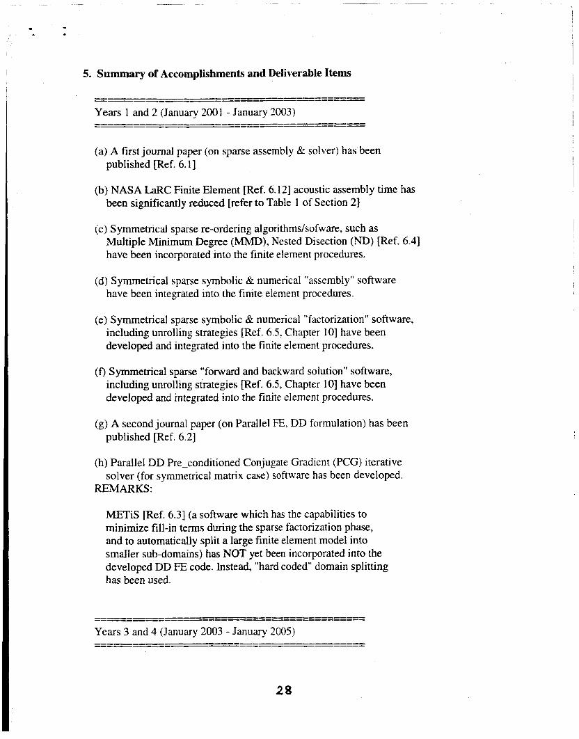
5. Summary of Accomplishments and Deliverable Items

(a) A first journal paper (on sparse assembly & solver) has been published [Ref. 6.11

(b) NASA LaRC Finite Element [Ref. 6.121 acoustic assembly time has been significantly reduced [refer to Table 1 of Section 21

(c j S ymmetricai sparse re-ordering algorithms/sofware, such as Multiple Minimum Degree (MMD), Nested Disection (ND) [Ref. 6.41 have been incorporated into the finite element procedures.

(d) Symmetrical sparse symbolic & numerical "assembly" software have been integrated into the finite element procedures.

(e) Symmetrical sparse symbolic & numerical "factorization" software, including unrolling strategies [Ref. 6.5, Chapter 101 have been developed and integrated into the finite element procedures.

(f) Symmetrical sparse "forward and backward solution" software, including unrolling strategies [Ref. 6.5, Chapter lo] have been developed and integrated into the finite element procedures.

(g) A second journal paper (on Parallel FE. DD formulation) has been published [Ref. 6.21

(h) Parallel DD Pre-conditioned Conjugate Gradient (PCG) iterative solver (for symmetrical matrix case) software has been developed.

REMARKS:

METiS [Ref. 6.31 (a software which has the capabilities to minimize fill-in terms during the sparse factorization phase, and to automatically split a large finite element model into smaller sub-domains) has NOT yet been incorporated into the developed DD FE code. Instead, "hard coded" domain splitting has been used.

28

(i) Un-symmetrical sparse symbolic & numerical "assembly" software have been integrated into the finite element procedures.

(i) Un-symmetrical sparse symbolic & numerical "factorization" software, including unrolling strategies [Ref. 6.5, Chapter 101 have been developed and integrated into the finite element procedures.

(k) Un-symmetrical sparse "forward and backward solution" software, including unrolling strategies have been developed and integrated into the finite element procedures.

(1) METiS [Ref. 6.31 (a software which has the capabilities to minimize fiii-in terms during the sparse factorization phase. and to automatically split a large finite element model into smaller sub-domains) has recently been incorporated into the developed DD FE code.

(m) Parallel DD [Ref. 6.61 Pre-conditioned Bi-CG iterative solver [Ref. 6-71 (for un-symmetrical matrix case] software has been developed.

However, the Bi-CG iterative solver (with DD formulation) and its communication strategies (amongst different processors) need further studies to improve the robustness of the algorithms !

REMARKS:

"Extra" works to investigate the possibilities of using the software MA28 [see Ref. 6.101, seperating the factorized and forwardhackward phases in the sparse solver package SUPER-LU [see Ref. 6.91 etc ... have also been conducted by Dr. Nguyen's (PI'S) research team at Old Dominon University (ODU) during the grant periods.

2 9

6. References

[6. I] W.R. Watson, D.T. Nguyen. C.J. Reddy, V.N. Vatsa, and W.H. Tang, "Algorithms and Application of Sparse Matrix Assembly and Equation Solvers for Aeroacoustics", AIAA Journal, Volume 40, KO. 4, pages 66 1-670 (Apri1'2002)

[6.2] D.T. Nguyen, W.R. Watson. S. Tungkahotara, and S.D. Rajan, "Parallel Finite Eiemenr Domain Decomposition for StructuraVAcoustic Analysis", Journal of Computational and Applied Mechanics. Vol. 4, No. 2, pages 189-201 (2003).

[6.3] Karypis, G., and Kumar, V.. "ParMETiS: Parallel Graph Patitioning and Sparse Matrix Ordering Library", University of Minnesota, Department of Computer Science, Version 2.0, 1998.

[6.4] George, J.A., and Liu, W.H.. Computer Solution of Large Sparse Positive Definite Systems, Prentice-Hall, Englewood Cliffs, NJ ( 198 1 )

[6.5] Nguyen,Duc T.,"Parallel-Vector Equation Solvers for Finite Element Engr. Applications", by Kluwer/Plenum Academics Publisher (2002)

[6.6] Nguyen,Duc T., "Finite Element Methods: Parallel-Sparse Statics and Eigen-Solutions". Graduate level textbook, Expected date of completion: April 28,2005

[6.7] R. Barrett, M. Berry, T. Chan. J. Demmel, J. Donato, J. Dongara, V. Eighout, R. Pozo. C . Romine, and H.V. der Vorst, "Templates for the Solution of Linear Systems: Building Blocks for Iterative Methods". SIAM, 1994

[6.8] Arora, J.S. and Nguyen, D.T., "Eigen-solution for Large Structural Systems with Substructures", International Journal for Numerical Methods in Engineering, Vol. 15, 1980, pp. 333-341.

[6.9] J.W. Demmel, J.R. Gilbert. and X.S. Li, "SuperLU Users' Guide", September 2 1, 1999

30

16. IO] I.S. Duff, "MA28-a set of FORTRAN subroutines for solving sparse unsymmetric sets of linear equations". Technical Report R.8730, AEFE, Harwell, England, 1982

16.1 11 SGI (library subroutines) sparse solver

E6.121 W.R. Watson, "Three-Dimensional Rectangular Duct Code With Application to Impedance Eduction", AIAA Journal, 40, pp. 2 17-226 (2002)

31

7. Acknowledgements

The PI (Duc T. Nguyen) would like to express his appreciation for the financial supports, provided by the NASA Langley Research Center, of this project. Dr. Willie Watson (at NASA LaRC), not only served a super job as a Technical Monitor, but he has also actively involved in the contributions of some of his "finite element acoustic subroutines", and providing many useful inputs, discussions during the verification phase of the developed codes.

The PI also expresses his appreciation for the contributions from several members of his ODU research team, such as Mr. Tungkahotara (Ph.D student), Dr. J. Qin (former Post-Doctoral Research Associate), and Dr. H. Runesha (former Ph.D student).

Finally, the computer facilities provided by NASA Langley Research Center. and Old Dominion University (OCCS) are also greatfully acknowledged.