Image Segmentation: the Mumford Shah functionalmatilde/MumfordShahSlides.pdf · Image Segmentation: the Mumford{Shah functional Matilde Marcolli and Doris Tsao Ma191b Winter 2017

Image Segmentation: the Mumford–Shahfunctional

Matilde Marcolli and Doris Tsao

Ma191b Winter 2017Geometry of Neuroscience

Matilde Marcolli and Doris Tsao Image Segmentation: the Mumford–Shah functional

References for this lecture:

David Mumford, Jayant Shah, Optimal Approximations byPiecewise Smooth Functions and Associated VariationalProblems, Commun. Pure Applied Math. Vol. XLII (1989)577–685.


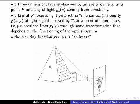
• a three-dimensional scene observed by an eye or camera: at apoint P intensity of light g1(ρ) coming from direction ρ

• a lens at P focuses light on a retina R (a surface): intensityg(x , y) of light signal received by R at a point of coordinates(x , y); obtained from g1(ρ) through some transformation thatdepends on the functioning of the optical system

• the resulting function g(x , y) is “an image”


• there will be discontinuities in the function g(x , y): boundaries(an object in front of another, objects with a common boundary,discontinuities in illumination, in the object albedo, etc.)

• additional complications:

textured objects, fragmented objects (eg a canopy of leaves)

shadows, penumbra

surface markings

partially transparent objects

noisy measurements of g(x , y)


Segmentation Problem

• goal: compute a decomposition

R = R1 ∪ · · · ∪ Rn

of the domain of g(x , y) such that

1 the function g(x , y) is smooth within each domain Ri

2 the function g(x , y) varies discontinuously (and/or veryrapidly) across most of the boundary between different Ri

• equivalently: problem of computing optimal approximations of afunction g(x , y) by piecewise smooth functions


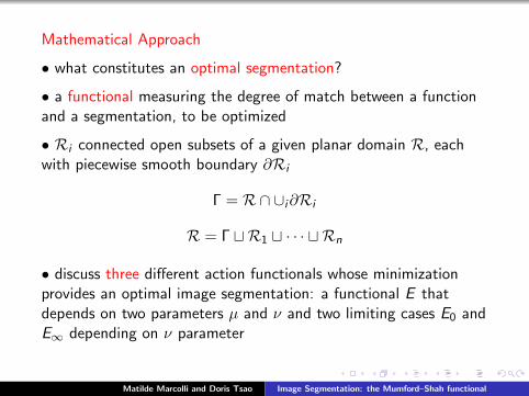
Mathematical Approach

• what constitutes an optimal segmentation?

• a functional measuring the degree of match between a functionand a segmentation, to be optimized

• Ri connected open subsets of a given planar domain R, eachwith piecewise smooth boundary ∂Ri

Γ = R∩ ∪i∂Ri

R = Γ tR1 t · · · t Rn

• discuss three different action functionals whose minimizationprovides an optimal image segmentation: a functional E thatdepends on two parameters µ and ν and two limiting cases E0 andE∞ depending on ν parameter


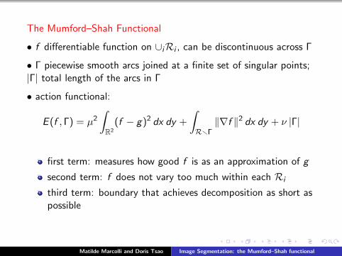
The Mumford–Shah Functional

• f differentiable function on ∪iRi , can be discontinuous across Γ

• Γ piecewise smooth arcs joined at a finite set of singular points;|Γ| total length of the arcs in Γ

• action functional:

E (f , Γ) = µ2

∫R2

(f − g)2 dx dy +

∫RrΓ‖∇f ‖2 dx dy + ν |Γ|

first term: measures how good f is as an approximation of g

second term: f does not vary too much within each Ri

third term: boundary that achieves decomposition as short aspossible


• Note: need all these terms to have nontrivial minimum

1 without first term: f = 0 and Γ = ∅ give E = 0

2 without second term: f = g and Γ = ∅ give E = 0

3 without third term: f average of g on a grid of N2 squareshas limit to E = 0

• heuristic interpretation: a solution f of the minimization of E isa “cartoon” version of the image g where contours are drawnsharply and scene is simplified

• Question: is the minimization problem for E well posed?Mumford and Shah conjectured: for all continuous g a minimumof E exists with f differentiable on each Ri and Γ made of C1-arcsjoined at a finite number of singular points


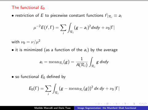
The functional E0

• restriction of E to piecewise constant functions f |Ri≡ ai

µ−2E (f , Γ) =∑i

∫Ri

(g − ai )2dxdy + ν0|Γ|

with ν0 = ν/µ2

• it is minimized (as a function of the ai ) by the average

ai = meanRi(g) =

1

A(Ri )

∫Ri

g dxdy

• so functional E0 defined by

E0(Γ) =∑i

∫Ri

(g −meanRi(g))2 dx dy + ν0 |Γ|


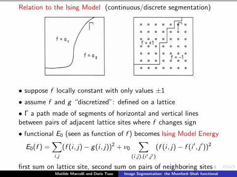
Relation to the Ising Model (continuous/discrete segmentation)

• suppose f locally constant with only values ±1

• assume f and g “discretized”: defined on a lattice

• Γ a path made of segments of horizontal and vertical linesbetween pairs of adjacent lattice sites where f changes sign

• functional E0 (seen as function of f ) becomes Ising Model Energy

E0(f ) =∑i ,j

(f (i , j)− g(i , j))2 + ν0

∑(i ,j),(i ′,j ′)

(f (i , j)− f (i ′, j ′))2

first sum on lattice site, second sum on pairs of neighboring sitesMatilde Marcolli and Doris Tsao Image Segmentation: the Mumford–Shah functional

The Functional E∞

• a functional of Γ

E∞(Γ) =

∫Γ

(ν∞ −

(∂g

∂n

)2)

ds

ν∞ a constant, ds arc length on Γ, unit normal ∂/∂n along Γ

• minimizing E∞ means finding Γ so that

length of Γ is as short as possiblevariation of g in the direction normal to Γ is as large aspossible


Relation of E∞ to E

• smooth parts of Γ, curvilinear coordinates (s, r)

• take f = g outside a tubular neighborhood of Γ

• set µ = 1/ε and ν = 2εν∞ and

f (r , s) = g(r , s) + ε sign(r) e−|r |/ε∂g

∂r(0, s)

• thenE (f , Γ)− E (g , Γ) = 2εE∞(Γ) + O(ε2)

so can think of E∞ as a µ→∞ limit of E


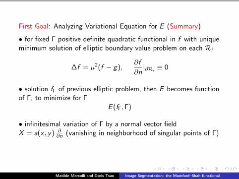
First Goal: Analyzing Variational Equation for E (Summary)

• for fixed Γ positive definite quadratic functional in f with uniqueminimum solution of elliptic boundary value problem on each Ri

∆f = µ2(f − g),∂f

∂n|∂Ri≡ 0

• solution fΓ of previous elliptic problem, then E becomes functionof Γ, to minimize for Γ

E (fΓ, Γ)

• infinitesimal variation of Γ by a normal vector fieldX = a(x , y) ∂

∂n (vanishing in neighborhood of singular points of Γ)


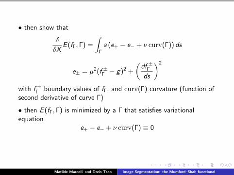
• then show that

δ

δXE (fΓ, Γ) =

∫Γa (e+ − e− + ν curv(Γ)) ds

e± = µ2(f ±Γ − g)2 +

(df ±Γds

)2

with f ±Γ boundary values of fΓ, and curv(Γ) curvature (function ofsecond derivative of curve Γ)

• then E (fΓ, Γ) is minimized by a Γ that satisfies variationalequation

e+ − e− + ν curv(Γ) ≡ 0


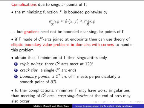
Complications due to singular points of Γ:

• the minimizing function fΓ is bounded pointwise by

minR

g ≤ fΓ(x , y) ≤ maxR

g

... but gradient need not be bounded near singular points of Γ

• if Γ made of C2-arcs joined at endpoints then can use theory ofelliptic boundary value problems in domains with corners to handlethis problem

• obtain that if minimum at Γ then singularities only

1 triple points: three C2 arcs meet at 120

2 crack tips: a single C2 arc ends

3 boundary points: a C2 arc of Γ meets perpendicularly asmooth point of ∂R

• further complications: minimizer Γ may have worst singularitiesthan meeting of C2 arcs: cusp singularities at the end of arcs mayalso occur


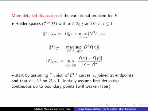
More detailed discussion of the variational problem for E

• Holder spaces Ck,α(Ω) with k ∈ Z≥0 and 0 < α ≤ 1

‖f ‖Ck,α = ‖f ‖Ck + max|β|=k

|Dβf |C0,α

‖f ‖Ck = max|β|≤k

supx∈Ω|Dβf (x)|

‖f ‖C0,α = supx 6=y∈Ω

|f (x)− f (y)||x − y |α

• start by assuming Γ union of C1,1 curves γa joined at endpointsand that f ∈ C1 on Rr Γ, initially assume first derivativecontinuous up to boundary points (will weaken later)


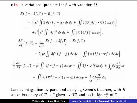
• fix Γ: variational problem for f with variation δf

Last by integration by parts and applying Green’s theorem, with Bwhole boundary of Rr Γ given by ∂R and each side γ±a of Γ


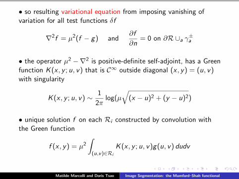
• so resulting variational equation from imposing vanishing ofvariation for all test functions δf

∇2f = µ2(f − g) and∂f

∂n= 0 on ∂R∪a γ±a

• the operator µ2 −∇2 is positive-definite self-adjoint, has a Greenfunction K (x , y ; u, v) that is C∞ outside diagonal (x , y) = (u, v)with singularity

K (x , y ; u, v) ∼ 1

2πlog(µ

√(x − u)2 + (y − u)2)

• unique solution f on each Ri constructed by convolution withthe Green function

f (x , y) = µ2

∫(u,v)∈Ri

K (x , y ; u, v)g(u, v) dudv


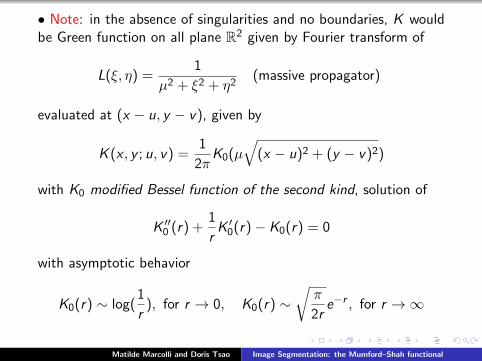
• Note: in the absence of singularities and no boundaries, K wouldbe Green function on all plane R2 given by Fourier transform of

L(ξ, η) =1

µ2 + ξ2 + η2(massive propagator)

evaluated at (x − u, y − v), given by

K (x , y ; u, v) =1

2πK0(µ

√(x − u)2 + (y − v)2)

with K0 modified Bessel function of the second kind, solution of

K ′′0 (r) +1

rK ′0(r)− K0(r) = 0

with asymptotic behavior

K0(r) ∼ log(1

r), for r → 0, K0(r) ∼

√π

2re−r , for r →∞


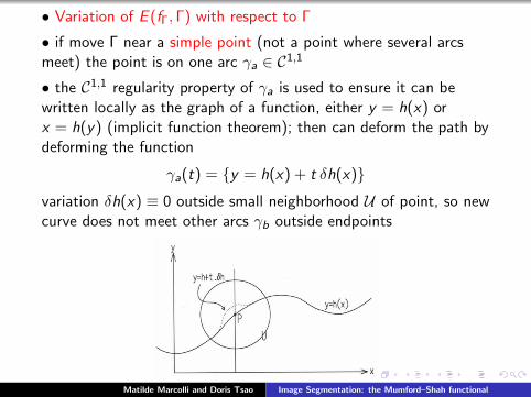
• Variation of E (fΓ, Γ) with respect to Γ

• if move Γ near a simple point (not a point where several arcsmeet) the point is on one arc γa ∈ C1,1

• the C1,1 regularity property of γa is used to ensure it can bewritten locally as the graph of a function, either y = h(x) orx = h(y) (implicit function theorem); then can deform the path bydeforming the function

γa(t) = y = h(x) + t δh(x)variation δh(x) ≡ 0 outside small neighborhood U of point, so newcurve does not meet other arcs γb outside endpoints


• Note: varying Γ forces f to vary too because f ∈ C1 of Rr Γand discontinuous across Γ

• U+ = (x , y) : y > h(x) ∩ U and U−(x , y) : y > h(x) ∩ Uand f ± = f |U± extend both f ± to all U with a C1 extension f ±

f t(x , y) =

f (x , y) (x , y) /∈ U

f +(x , y) (x , y) ∈ U , above γa(t)

f −(x , y) (x , y) ∈ U , below γa(t)

• then compute explicitly variation E (f t , Γ(t))− E (f , Γ) whereΓ(t) = γa(t) ∪b 6=a γb


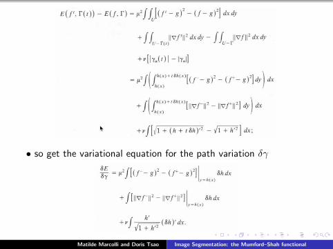
• so get the variational equation for the path variation δγ


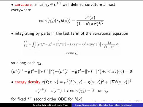
• curvature: since γa ∈ C1,1 well defined curvature almosteverywhere

curv(γa)(x , h(x)) =h′′(x)

(1 + h′(x)2)3/2

• integrating by parts in the last term of the variational equation

so along each γa

(µ2(f +−g)2+‖∇f +‖2)−(µ2(f −−g)2+‖∇f −‖2)+ν curv(γa) = 0

• energy density e(f ; x , y) = µ2(f (x , y)− g(x , y))2 + ‖∇f (x , y)‖2

e(f +)− e(f −) + ν curv(γa) = 0 on γa

for fixed f ± second order ODE for h(x)Matilde Marcolli and Doris Tsao Image Segmentation: the Mumford–Shah functional

Special points of Γ: more complicated analysis of the variationalproblem (restrictions at these points imposed by stationarycondition for the functional E )

• Cases:

1 points where Γ meets ∂R2 corners where two γa arcs meet

3 vertices where three or more γa meet

4 crack-tips where a γa ends without meeting another arc


• Problem with corners: can have a function ∇2f = 0 in openregion, ∂f

∂n = 0 on boundary, with singularity at corner point

f (z) = =(w) = rπ/α sin(π

αθ)

for z = re iθ and w = zπ/α (conformal map that flattens corner)

then

∂f

∂r=π

αrπα−1 sin(

π

αθ)→∞ when r → 0, if α > π


Elliptic boundary value problems on domains with corners(Kondratiev)

• previous example is typical behavior of solutions of ellipticboundary value problems in domains with corners: solutions fsatisfy

f bounded everywhere

f is C1 at corners with angle 0 < α < π

at corners with π < α ≤ 2π (case 2π is crack-tip)

f = crπ/α sin(π

α(θ − θ0)) + f

with f ∈ C1


• use this to show that Mumford–Shah minimizers cannot havekinks (two-arcs corners with angle 6= π)

Divide neighbor into sectors with angle larger/smaller than π; takesmooth cutoff function ηU on a ball near corner


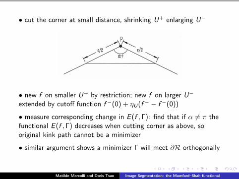
• cut the corner at small distance, shrinking U+ enlarging U−

• new f on smaller U+ by restriction; new f on larger U−

extended by cutoff function f −(0) + ηU(f − − f −(0))

• measure corresponding change in E (f , Γ): find that if α 6= π thefunctional E (f , Γ) decreases when cutting corner as above, sooriginal kink path cannot be a minimizer

• similar argument shows a minimizer Γ will meet ∂R orthogonally


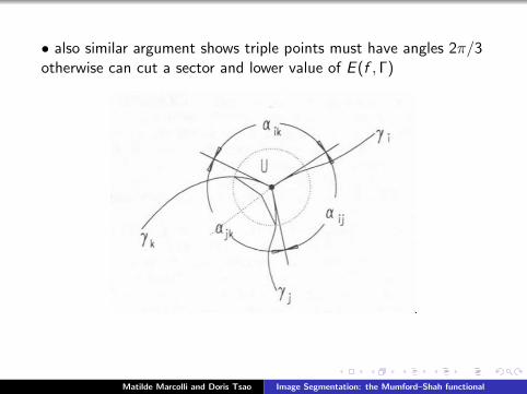
• also similar argument shows triple points must have angles 2π/3otherwise can cut a sector and lower value of E (f , Γ)


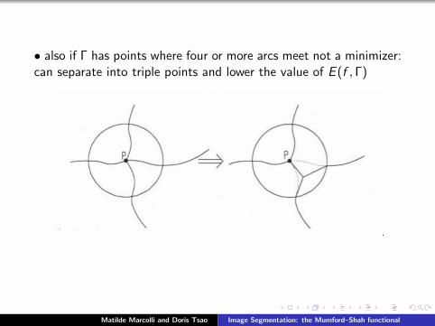
• also if Γ has points where four or more arcs meet not a minimizer:can separate into triple points and lower the value of E (f , Γ)


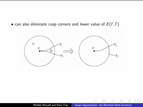
• can also eliminate cusp corners and lower value of E (f , Γ)


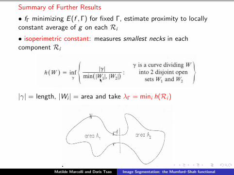
Summary of Further Results

• fΓ minimizing E (f , Γ) for fixed Γ, estimate proximity to locallyconstant average of g on each Ri

• isoperimetric constant: measures smallest necks in eachcomponent Ri

|γ| = length, |Wi | = area and take λΓ = mini h(Ri )


domain with isoperimetric constant h(Ri ) = 0

• small µ limit: prove estimate

µ2

(E0(Γ)− 4µ2

λ2Γ + 4µ2

‖g‖20,2,R

)≤ E (fΓ, Γ) ≤ µ2E0(Γ)


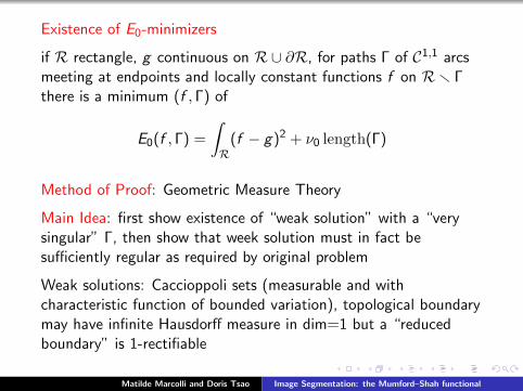
Existence of E0-minimizers

if R rectangle, g continuous on R∪ ∂R, for paths Γ of C1,1 arcsmeeting at endpoints and locally constant functions f on Rr Γthere is a minimum (f , Γ) of

E0(f , Γ) =

∫R

(f − g)2 + ν0 length(Γ)

Method of Proof: Geometric Measure Theory

Main Idea: first show existence of “weak solution” with a “verysingular” Γ, then show that week solution must in fact besufficiently regular as required by original problem

Weak solutions: Caccioppoli sets (measurable and withcharacteristic function of bounded variation), topological boundarymay have infinite Hausdorff measure in dim=1 but a “reducedboundary” is 1-rectifiable


What is Geometric Measure Theory?

• use of measure theory methods to study geometric objects(curves, surfaces) that are highly non-smooth

• historically developed to study the Plateau Problem (thegeometry of soap bubble film: area minimizing surfaces with givenboundary curves)

• Introduction to Geometric Measure Theory:

Frank Morgan, Geometric measure theory: A beginner’s guide(Fourth ed.), Academic Press, 2009.

Frederick J. Almgren, Jr., Plateau’s Problem: An Invitation toVarifold Geometry, Revised Edition, American MathematicalSociety, 2001.

Herbert Federer, Colloquium lectures on geometric measuretheory, Bull. Amer. Math. Soc. 84 (1978), 291–338


Plateau Problem (images by John M. Sullivan)

in “Plateau’s Problem” by Frederick J. Almgren, Jr


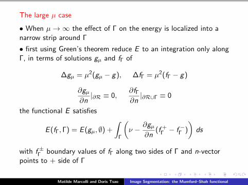
The large µ case

• When µ→∞ the effect of Γ on the energy is localized into anarrow strip around Γ

• first using Green’s theorem reduce E to an integration only alongΓ, in terms of solutions gµ and fΓ of

∆gµ = µ2(gµ − g), ∆fΓ = µ2(fΓ − g)

∂gµ∂n|∂R ≡ 0,

∂fΓ∂n|∂R∪Γ ≡ 0

the functional E satisfies

E (fΓ, Γ) = E (gµ, ∅) +

∫Γ

(ν − ∂gµ

∂n(f +

Γ − f −Γ )

)ds

with f ±Γ boundary values of fΓ along two sides of Γ and n-vectorpoints to + side of Γ


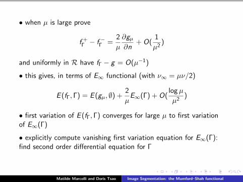
• when µ is large prove

f +Γ − f −Γ =

2

µ

∂gµ∂n

+ O(1

µ2)

and uniformly in R have fΓ − g = O(µ−1)

• this gives, in terms of E∞ functional (with ν∞ = µν/2)

E (fΓ, Γ) = E (gµ, ∅) +2

µE∞(Γ) + O(

logµ

µ2)

• first variation of E (fΓ, Γ) converges for large µ to first variationof E∞(Γ)

• explicitly compute vanishing first variation equation for E∞(Γ):find second order differential equation for Γ


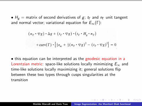
• Hg = matrix of second derivatives of g ; tΓ and nΓ unit tangentand normal vector; variational equation for E∞(Γ):

• this equation can be interpreted as the geodesic equation in aLorentzian metric: space-like solutions locally minimizing E∞ andtime-like solutions locally maximizing it; general solutions flipbetween these two types through cusps singularities at thetransition


A lot of more recent results on Mumford-Shah minimizers andsegmentation: rich current area of research; a large number ofpapers available on the topic

Suggested References:

Laurent Younes, Peter W. Michor, Jayant Shah, DavidMumford, A metric on shape space with explicit geodesics,Rend. Lincei Mat. Appl. 19 (2008) 25–57

Mumford, D.; Kosslyn, S. M.; Hillger, L. A.; Herrnstein, R. J.Discriminating figure from ground: the role of edge detectionand region growing, Proc. Nat. Acad. Sci. U.S.A. 84 (1987),no. 20, 7354–7358.

Leah Bar et al. Mumford and Shah Model and itsApplications to Image Segmentation and Image Restoration,in “Handbook of Mathematical Methods in Imaging”,Springer 2011, 1095–1157


Documents

Image Segmentation: the Mumford Shah functionalmatilde/MumfordShahSlides.pdf · Image Segmentation: the Mumford{Shah functional Matilde Marcolli and Doris Tsao Ma191b Winter 2017