IEEE TRANSACTIONS ON COMPUTERS 1 Malware-on-the-Brain

THIS PAPER HAS BEEN ACCEPTED BY IEEE TRANSACTIONS ON COMPUTERS FOR FINAL PUBLICATION IN AN UPCOMING ISSUE 1

Malware-on-the-Brain: Illuminating Malware ByteCodes with Images for Malware Classification

Fangtian Zhong, Zekai Chen, Minghui Xu, Guoming Zhang, Dongxiao Yu, Xiuzhen Cheng, Fellow, IEEE

Abstract—Malware is a piece of software that was written with the intent of doing harm to data, devices, or people. Since a number ofnew malware variants can be generated by reusing codes, malware attacks can be easily launched and thus become common inrecent years, incurring huge losses in businesses, governments, financial institutes, health providers, etc. To defeat these attacks,malware classification is employed, which plays an essential role in anti-virus products. However, existing works that employ eitherstatic analysis or dynamic analysis have major weaknesses in complicated reverse engineering and time-consuming tasks. In thispaper, we propose a visualized malware classification framework called VisMal, which provides highly efficient categorization withacceptable accuracy. VisMal converts malware samples into images and then applies a contrast-limited adaptive histogramequalization algorithm to enhance the similarity between malware image regions in the same family. We provided a proof-of-conceptimplementation and carried out an extensive evaluation to verify the performance of our framework. The evaluation results indicate thatVisMal can classify a malware sample within 4.0 ms and have an average accuracy of 96.0%. Moreover, VisMal provides securityengineers with a simple visualization approach to further validate its performance.

Index Terms—Classification; Histogram Equalization; Malware; Visualization.

F

1 INTRODUCTION

MALWARE classification refers to the process of group-ing malware samples with similar features to effec-

tively classify unknown malware. Features can be catego-rized as either static or dynamic, with the former beingextracted based on a byte-code sequence, binary assemblyinstructions, or an imported Dynamic Link Library (DLL),and the latter on runtime file system activities, terminalcommands, network communications, and function or sys-tem call sequences. Since malware samples in the samefamily normally have similar static or dynamic features,which could be extracted via machine learning algorithms,security vendors and researchers usually utilize them asuseful clues for effective malware classification [1], [2].

However, malware feature extraction, whether static ordynamic, is a non-trivial task. The extraction of static fea-tures requires security professionals to have a good com-mand of the structure of malware binaries. For instance, toextract an imported Dynamic Link Library in a Windowsprogram, developers have to know the PE before parsingtwo structures in the order of DataDirectories followedby Import or Import Address Table [3]. Additionally, it iseven worse when encryption or compression is applied tomalware binaries as reverse analysis is needed [4]. On theother hand, although the extraction of dynamic featuresobviates the conundrums and limitations of static feature

• Fangtian Zhong and Zekai Chen are with the Department of ComputerScience, The George Washington University, Washington DC, USA.Emails: {squareky zhong,zech chan}@gwu.edu

Minghui Xu, Guoming Zhang, Dongxiao Yu and Xiuzhen Cheng(Corresponding Author) are with the School of Computer Science andTechnology, Shandong University, Qingdao, 266237, China. Emails:{mhxu,guomingzhang,dxyu,xzcheng}@sdu.edu.cn

extraction, dynamic analysis can only collect the behaviorsof specific execution paths since it is hardly possible totraverse all of them. Meanwhile, dynamic analysis is time-consuming. For instance, some applications may have mul-tiple event handlers that should be examined for dynamicfeature extraction. Nevertheless, it can be insufficient tocall just the one that contains a particular API invocation;instead, multiple event handlers may need to be triggeredas a “chain” in a particular order with specific inputs [5].

One can see from the above analysis that malware clas-sification involves either very high knowledge barriers forsecurity professionals or huge computing burdens for com-puters. To overcome the knowledge obstacles and improvemalware classification efficiency, we have to address thefollowing three critical challenges when designing malwareclassification schemes. First, since the ultimate purpose ofmalware classification is to precisely classify different mal-ware samples, the extracted features should uniquely rep-resent the samples and maintain the similarity for malwarein the same family. Second, as the schemes are expected tobe efficient, the time for extracting features and classifyingmalware samples should be limited to some degree thatusers can withstand. Third, even though security engineersmay not have enough background knowledge about mal-ware samples, the schemes should be easy to use andcomprehend. Based on these considerations, we present anovel but simple visualized classification framework namedVisMal in this paper, which aims at understanding the innerworkings of malware families and disclosing the encodingart in the byte codes of malware binaries. VisMal consists ofthree major components: Converter, Feature Engineer, andClassifier. Converter takes charge of converting a malwaresample into a 2-Dimensional grayscale image; Feature Engi-neer enhances the recognition of malware via strengtheningthe local contrast in the malware image regions and resizes

arX

iv:2

108.

0431

4v3

[cs

.CR

] 9

Mar

202

2


the image to a smaller one to expedite the classificationprocess; and Classifier is used to partition malware samplesinto their corresponding families.

VisMal endeavors to greatly reduce the burdens onsecurity engineers and the computing expenses on com-puters. Since existing works adopt either static or dynamicanalysis approaches, which inevitably have drawbacks asmentioned above, it is necessary to turn our mind to pursuethe essence of the malware families themselves. Note thatmany variants of malware samples are generated by reusingcore codes [6]–[9], one can use the similarity of instructionsequences to classify different types of malware samples. Weprovide an implementation of VisMal and conduct extensiveexperimental studies to evaluate its effectiveness in termsof accuracy, efficiency, and visualization. This study makesevery effort to understand malware families and discoverthe underlying encoding art in byte codes. Our multi-foldcontributions can be summarized as follows.

1) We propose VisMal, a visualized malware classifica-tion framework, to efficiently distinguish differenttypes of malware samples while in the mean timemaintaining high accuracy.

2) By improving local contrasts of the regions in con-verted images, we enlarge the discernity of malwaresamples, which elevates the accuracy from grayscaleimages without extra operations.

3) When malware samples are compressed or en-crypted, VisMal still demonstrates good perfor-mance on distinguishing different malware families.

4) VisMal provides a visual technique for security en-gineers without much knowledge about malwaresamples to readily validate the classification perfor-mance.

The rest of the paper is organized as follows. Section 2introduces the most related work. Section 3 details the work-flow and implementation of VisMal. Section 4 evaluates theperformance of VisMal, and Section 5 concludes the paperwith a discussion on future research.

2 RELATED WORK

In this section, we provide an overview on popular existingmalware classification methods, considering whether theyare static analysis based or dynamic analysis based.

2.1 Malware Classification Based on Static AnalysisSince static features can be directly obtained from malwarefiles without execution but they still possess certain dis-cernibility, many approaches based on these features wereproposed to classify different malware families, which aresummarized as follows.

Machine Learning-Based Approaches. Jiang et al. de-veloped a K Nearest Neighbour based (KNN) model formalware classification by taking an input vector carryingcodes’ semantic information that comes from sensitive op-code sequences [10]. Each sensitive opcode sequence isconstructed by opcodes, application programming inter-faces, STR instructions, and actions. All sensitive opcodesequences are sent to Doc2vec for the generation of sen-sitive semantic information, and the information is then

used for classification in a pretrained KNN model. Fasanoet al. proposed a cascade learning method to distinguishdifferent malware families by combining a KStar classifierfor the discrimination of benignware and malware with aRandomForest classifier for the identification of differentmalware families [11]. The cascade learner makes use oftotally 12 static values as features that are calculated fromeach malware, including cyclomatic complexity, weightedmethods per class, bad smell method calls, wakelocks withno timeout, number of location listeners, number of GPSusers, etc. Blanc et al. trained a random forest classifier byleveraging the architectural and external attributes of ma-licious apps to identify different android malware families[12]. To construct these attributes for a piece of malware, anapp is initially decompiled with Apktool and converted intohuman-readable Smali codes. These codes are then parsedby a code quality tool and finally used for the extraction of10 attributes (e.g., XML Parsers and Network Timeouts).

DNN-Based Approaches. Jung et al. proposed a convo-lutional neural network model based on byte informationto classify malware samples [13]. The extraction of byteinformation includes 3 steps: a malware binary file is firstinput to a disassembler, which returns the disassembledmalware file; then byte length sequences are extracted fromthe disassembled malware file and used as parameters to aspecific hash function; finally all hash values generated fromthe second step are used to construct a hash map, whichis referred to as the byte information. Saxe et al. presenteda deep feed forward neural network trained on variousfeatures extracted by static analysis for binary malwareclassification [14]. The features include system library im-port functions, ASCII printable strings, PE metadata fieldsin the executable, as well as byte sequences from the rawcodes. They are concatenated to form a 1024-dimensionalfeature vector, which is fed into a four-layer feed forwardnetwork for training and further classification. Davis et al.developed an approach that employs a convolutional neuralnetwork to identify malware [15]. The raw disassembledcodes of malware are processed to generate a vector of fixed-length features. This approach extracts the individual x86processor instructions with diverse lengths and then applypadding or truncation to create fixed length features. Thedisassembled codes are also parsed to extract system libraryimport functions to further extend the feature vector size.

Other Approaches. Kinable et al. investigated malwareclassification based on call graph clustering [16]. Each mal-ware can be represented as multiple call graphs that consistof local functions and system library functions as vertexesand caller-callee relationships as edges. Malware programsin the same family should have minimized number ofmismatchings in their graphs. To compute malware mis-matchings, they adopted the graph edit distance that isthe minimum number of elementary operations requiredto transform one graph to another. Mirzaei et al. proposeda characterization approach for malware families based oncommon ensembles of sensitive API calls [17]. The over-all architecture of the proposed system goes through fivesteps: it first computes fuzzy hash values of all functionsextracted from the apps in the same family; then it createscall graphs and uses the fuzzy hash values to replace thenodes (functions); next, it merges the hashed call graphs and


all edges to form an aggregated graph and assigns a uniqueweight to each edge; following that it inspects the resultsfrom the frequency of similar methods and the frequencyof the methods’ invocations in the similar methods withina family, which are used to create feature vectors at lastfor classification. Zhang et al. implemented a prototypesystem named DroidSIFT, a novel semantic-based approachto classify Android malware via dependency graphs [18].They generated dependency graphs by discovering entrypoints and analyzing call graphs. Following the generationof dependency graphs, they leveraged both forward andbackward dataflow analysis to explore API dependenciesand uncover constant parameters. DroidSIFT hence usesdependency graphs to build graph databases and classifies amalware sample by producing graph-based feature vectorsand then performing graph similarity queries.

2.2 Malware Classification Based on Dynamic Analysis

In contrast to static analysis, which derives properties froma program’s text, dynamic analysis obtains properties by ex-amining a running program. Approaches based on dynamicanalysis are important complements to improve detectivecapability when static features are hard to extract due to ob-fuscations. In this subsection, we summarize major malwareclassification works based on dynamic analysis.

Machine Learning Based Approaches. Sethi et al. de-veloped a machine learning based malware analysis frame-work for classification [19]. All malware samples are exe-cuted and analyzed on top of the Cuckoo Sandbox, whichexamines their run-time behaviors and returns behavioralreports that memorize their activities. The reports are fur-ther processed by a feature extraction and selection modulebefore sent to machine learning models such as DecisionTree and Random Forest for final classification. In [20],Martin et al. implemented a tool termed CANDYMAN toclassify Android malware by combining dynamic analysisand Markov chains. In their experiment, DroidBox wasemployed as the dynamic analysis tool to generate a statesequence representation for each malware. The state se-quence representation is then used to model the transitionprobabilities between consecutive states. Once all transitionprobabilities are computed, they are input to a collectionof machine learning algorithms (i.e., SMOTE, Random OverSampler, Random Under Sampler, etc.) for further classi-fication. Anderson et al. designed a malware classificationalgorithm based on graphs constructed from dynamicallycollected instruction traces of target execuables under theEther system [21]. Each instruction is denoted as a vertexin a graph, an edge between two nodes represents thetransition from one instruction to another, and the transi-tion probabilities are estimated by all collected traces. Onecan acquire a similarity matrix with each entry describingthe similarity between an executable and a malware class,which is obtained by employing graph kernels, and thensend the matrix to a support vector machine for classifica-tion.

DNN-Based Approaches. Dahl et al. trained a neuralnetwork with three hidden layers by feeding it with systemAPI calls as well as null terminated strings extracted fromthe process memory [22]. A random projection technique

was used to reduce the features’ dimensionality to thedegree that is manageable by the neural network. Tobiyamaet al. developed a recurrent neural network (RNN) to extractfeatures from a detailed representation of malware processbehaviors and used a convolutional neural network (CNN)to classify the outputs from the RNN [23]. Each API callrepresents an operation of the process, multiple API callsrepresent an activity, and multiple activities represent abehavior of the process. In each operation, critical infor-mation such as process name, ID, event name, and pathof current directory is recorded. Zhang et al. proposed alow-cost feature extraction approach and an effective deepneural network architecture for accurate and fast malwareclassification [24]. They executed PE files inside virtualmachines and used API hooks to monitor the API calltraces. They also utilized a feature hashing trick to encodethe API call arguments associated with the API name foreach API call. The deep neural network architecture appliesmultiple Gated-CNNs to transform the encoding into par-ticular feature representations that are further processed bybidirectional LSTM (long-short term memory networks) tolearn the sequential correlations among API calls.

Other Approaches. Vij et al. proposed a novel graphsignature based malware classification mechanism [25]. Thegraph signature uses sensitive application programminginterfaces to capture the control flow that builds a bridge be-tween sensitive APIs and the respective incidents. A datasetof graph signatures for well-known malware families is thencreated. A new application’s graph signature is comparedwith the signatures in the dataset, and the application isclassified into the corresponding malware family. Park et al.developed a malware classification algorithm called FACTvia finding the maximum common subgraphs in directedfunction call graphs [26]. Each graph is constructed bycapturing the uses of the system functions along with theparameter values when the malware program is executedin a sandboxed environment. Since malware programs be-longing to the same family generally share similar behaviorsby calling certain system functions, i.e., file system modifica-tion, new process spawning, network connectivity checking,registry modification, etc., their subgraphs tend to be similarto some extent. Hsiao et al. proposed an analysis scheme togroup Android malware based on their dynamic behaviors,and to identify the behaviors of a malware family. They alsoapplied phylogenetic tree, significant principal components,and dot matrix on different malware families to demonstratetheir behavioral correlations. The proposed methods canautomatically discover similar behaviors of different mal-ware groups, extract the characteristics of each malwaregroup, and provide security experts with the visualizedinformation based on runtime behaviors [27].

2.3 Summary

In this paper, we present VisMal, which converts malwarebinaries into 2-Dimensional grayscale images and utilizes acontrast-limited adaptive histogram equalization algorithmto expand the difference in all image regions such thatit is easier for our classifier to capture the similarity ofmalware samples in the same family. Previous works suchas [1], [2], [5], [11] perform less effective when reverse


MALWARE

Malware samples (1) Convert to images Imaged data(2) Apply contrast limited

adptive histogram equalization to images

(4) Apply CNN to resized images for classification

Predicted malware family

Adialer.C

C2LOP.P

Allaple.A Agent.FYI

Allaple.L Fakerean

...

1 0 1 1 01 1 0 11 010 0 1 10 10 10 0111 00 10 11 0 101 1 10 101 11 001 00 10 111 0 101 10 10 001 11 00

Convertor (3) Resize images to 64x64

Feature Engineer

Classifier

Fig. 1: Overview of the VisMal Framework

analysis is an obstacle and time is a constrained factor.VisMal cleverly bypasses the obstacles of reverse analysisby making effort to understand the properties of malwarefamilies, and discover the underlying similarity in bytecodes. Additionally, VisMal processes a malware programas an image, significantly reducing the waiting time foranalysis. These two features make VisMal more practicaland efficient. VisMal is also different from the works suchas [28]–[31] that process malware as images, which focuson statistical features of the converted image – VisMalpays attention to the understanding of the correspondencebetween byte codes and pixels. Besides, VisMal does notneed to intentionally pick out particular statistical featuresfor classification.

From the previous analysis, one can see that malwareclassification based on static features distinguishes differ-ent malware samples mainly by grouping their text andstatistical information extracted from malware files. Textinformation includes opcode sequences, system library im-port functions, and ASCII printable strings, while statisticalinformation calculated by various tools involves cyclomaticcomplexity, number of GPS users, and network timeouts,etc. Different from static analysis based methods, VisMaldoes not require the disasembling of the malware samplesand the help of any tool. On the other hand, malwareclassification based on dynamic features deals with therunning programs on top of virtual machines and examinesmalware samples by their programs’ activities, instructiontraces, API call traces, control flows, etc. In contrast tosuch methods, VisMal does not need to execute programsand check each execution trace to assure the reliability ofclassification. Besides, the selection of a distinct collectionof features to uniquely represent a malware sample is notrequired by VisMal.

3 THE PROPOSED VISMAL FRAMEWORK

3.1 Overview of VisMal

The three-fold objectives of VisMal include: i) efficientlyclassify malware samples into their respective families, ii)reduce security engineers’ burdens by providing automaticclassification tools, and iii) offer an image-based validationmethod for identifying the effectiveness of classification.The framework of VisMal is presented in Fig. 1. One can seethat VisMal consists of 3 components: Converter, Feature En-gineer, and Classifier. Converter converts a malware binaryinto an image. Feature Engineer processes the image by acontrast-limited adaptive histogram equalization algorithmto increase the local contrast in different image regionsand then resize the processed image to a smaller fixed-size one that can accelerate the process of classification.Classifier employs a shallow convolutional neural network-based model. It enables parameter sharing, a technique thatapplies the same small filter to all elements of the input andcaptures the correlation of different elements, to allow CNNto efficiently extract the local features in an image.

The workflow of VisMal is described as follows. Allmalware samples, whether in the training dataset or in thetest datasets, need to be converted to a grayscale imageaccording to the following procedure: a malware exampleis first sent to Converter for numeric conversion, whichoutputs an array consisting of numbers with scope between0 and 255; then the array is reshaped according to its file size(see Table 1); following the reshaping is the feature editingand resizing processes by Feature Engineer. The output ofFeature Engineer is an image array scaled to 64x64. Then it isconcatenated with the corresponding malware family label.The data is randomly divided into a training dataset and testdataset by StratifiedKFold. This is a variation of KFold thatreturns stratified folds made by preserving the percentage


of samples for each class [32]. The training dataset is usedto train Classifier. Once the classifier is well trained, onecan use it to characterize the malware samples in the testdataset.

TABLE 1: Correspondence between the file size of amalware sample and the converted image width

File Size Width Height≤ 10KB 32 (0, 312]

10KB-30KB 64 (156, 468]30KB-60KB 128 (234, 468]60KB-100KB 256 (234, 390]100KB-200KB 384 (260, 520]200KB-500KB 512 (390, 976]500KB-1000KB 768 (651, 1302]

1000KB ≤ 1024 (976,∞)

3.2 The Components of the VisMal Framwork

In this section, we detail the implementations of the threecomponents of VisMal, namely Converter, Feature Engineer,and classifier.

Malware Binary

Binaryto

decimal01010101=85

Imaged dataDecimal

2D Array

ReshapeDecimal

1D Array

Fig. 2: Converter

3.2.1 Converter

Fig. 2 demonstrates the procedure of numeric conversionby Converter for a malware example. To convert a malwarebinary into a grayscale image, Converter sequentially readsthe binary data in bytes, converts each byte into a decimalnumber ranging in [0-255] [28], then saves the number in aone-dimensional array. For instance, ’0110000’ is convertedto 96. Every number in the array corresponds to a pixel in agrayscale image. As the resolution of a grayscale image haswidth and height dimensions but different malware samplesvary in their file sizes, one should consider such a situationto accept diverse options of width and height. In this paper,we take a simple approach to reshape the image data (array)by following the recommended fixed-width with a variableheight according to its file size, which is correspondinglytransformed into a 2-Dimensional grayscale image conform-ing to portable network graphics (.png extension) via a built-in function, i.e., imwrite or imsave, in cv2 library or PILlibrary. The recommended fixed image widths for distinctmalware file sizes are given in Table 1 [29].

3.2.2 Feature Engineer

As suggested in [6]–[9], many variants of malware samplesare generated by reusing core codes. Therefore one can usethe similarity of instruction sequences to classify differentmalware samples. Since an instruction typically has multiplebytes and each byte corresponds to one pixel, the instructionis converted into several pixels by Converter. Thus locating

similar instruction sequences from different malware sam-ples is equivalent to identifying regions with similar pixelvalues in their corresponding images. Nevertheless, similarinstruction sequences from different malware samples be-longing to the same malware family may exist at differentpositions of their files. To overcome this challenge, we resortto the image contrast to identify similar pixel regions –image regions produced by similar instruction sequencesshould have similar contrast values. To further improve theaccuracy of Classifier, the capture of similar pixel valuesin different malware images should be promoted. Sincethe usable data of an image is normally represented byclose contrast pixel values [33], increasing the contrast ofan image benefits classification. Therefore, Feature Engineeradjusts pixel intensities in each image region to enhance thecontrast for a malware image by applying a contrast-limitedadaptive histogram equalization algorithm. This algorithmmaps the narrow range of input pixel values for an imageregion to the whole range of the pixel values for an image,i.e., 0-255. Through this adjustment, the intensities can bebetter distributed on the histogram1 for each image regionby effectively spreading out the most frequent intensityvalues, which allows for areas of lower contrast to gainhigher contrast and improves the contrast for the entireimage. High contrast enhances the possibility of Classifierto identify similar pixel values in images.

Figuratively speaking, contrast-limited adaptive his-togram equalization seems to be equivalent to signal trans-form that happens in biological neural networks so as tomaximize the output firing rate of a neuron which is afunction of the input statistics. The equalization algorithmcontains 4 phases: Division, Cumulation, Clipping, andTransformation. Division divides an image into a × b smallregions where a and b are respectively the numbers of piecessplit up for the width and height of the image. A cumulationis a cumulative frequency distribution function for an imageregion, whose computation is shown in (1):

cdf(i) =i∑

j=0

nj , 0 ≤ i < L (1)

where L is the total number of gray levels (typically 256),and nj is the number of times the pixel value j appears inan image region. Note that nj is also called the frequencyof j. As shown in Fig. 3, if the frequency of a pixel value isabove the threshold clipLimit, Clipping is applied to assigna random value in [0, 255] to some of such pixels such thatno pixel can have a frequency higher than clipLimit (seeFig. 3); correspondingly, the histogram is adjusted to a newfrequency distribution for the image region. Transformationtransforms the input pixel values into output pixel valuesby adopting different transformation methods according totheir positions in the malware image.

We use Fig. 4 as an example to illustrate the Transfor-mation phase. In Fig. 4, the image is partitioned into 4 × 3equal-sized rectangular regions. The center of each regionis represented by a black dot, and each boundary regionis partitioned into 4 smaller rectangles by the center lines,resulting in areas with three different colors (see Fig. 4).

1. a histogram correlates to the frequency distribution of pixel valuesfor an image region.


Pixel values0 255

Pixel values0 255

clipLimit clipLimit

Freq

uenc

y

Freq

uenc

y

Fig. 3: Clipping

P(x’, y’)

O(x, y)

a

N(x2, y2)

bR2(x2, y2)

Q22(x22, y22)

Q21(x21, y21)

M(x0, y0) R1(x1, y1)

Q11(x11, y11)

Q12(x12, y12)

Fig. 4: Transformation of Input Pixels

Each area includes the upper and left borders as well asthe outermost border of the image if it is a boundaryone. The input pixel values in the rectangle areas shadedpurple, sky blue, and pink are transformed by histogramequalization, linear interpolation, and bilinear interpolation,respectively. More specifically, according to [34], pixels inthe purple areas and the center pixel of each region aretransformed by histogram equalization; each pixel in thesky blue areas is transformed based on two collinear pixelsin the two neighboring purple areas by linear interpolation;and pixels in the pink area that lie between two collinearcenter pixels are transformed by linear interpolation whileother pink pixels are transformed by bilinear interpolationbased on the four neighboring center pixels. For example,consider the points M,N,Q11, Q12, Q21, Q22, O,R1, R2, Pin different areas of Fig. 4, where the value of the x-coordinate for each pixel point is the input pixel value, andthat of the y-coordinate is the output pixel value. The pointM in the purple area and the center points Q11, Q12, Q21,and Q22 of the four regions in the upper-left of the imageare transformed by histogram equalization according to thefollowing transformation function

y = hR(x) = round(cdf(x)− cdfmin

cdfmax − cdfmin×(L− 1)) (2)

over all the input pixel values in the image region the pointlies in to produce its output pixel value, where cdfmin isthe minimum non-zero value of the cumulative distribution

function calculated in the Cumulation phase while cdfmax

gives the maximum value.Note that (2) maps a narrow range of the input pixel

values to the full range of the image pixel values. However,this equation may overamplify the small amounts of noisesin largely homogeneous image regions [35]. For example, ifmost pixel values are big numbers, and noises’ pixel valuesare small numbers, the transformation of the noises may fallinto the same pixel value such that the noises are overam-plified as the frequency of the corresponding pixel valuesincreases. Clipping is thus adopted to equally redistributethe strongly peaked pixel values in the histogram in orderto limit the amplification of the noises when the frequency ofthe pixel values surpasses a prescribed threshold clipLimit.

On the other hand, a point O in the sky blue area locatedat the horizontal line MN , where M and N with pixelvalue x0 and x2, respectively, are points in the left-upperand right-upper corner purple areas of the image, can belinearly interpolated as follows:

y =x2 − x

x2 − x0hRM

(x0) +x− x0

x2 − x0hRN

(x2) (3)

Besides, point P , an arbitrary point in the pink area, is bi-linearly interpolated: its input pixel value x′ is transformedto the output pixel value y′ based on the input pixel valuesand output pixel values of the four neighboring centerpoints (Q11, Q12, Q21, and Q22) according to equations (4),(5), and (6). Specifically, (4) and (5) respectively compute theoutput pixel values of R1 and R2, which are then employedby (6) to generate the output pixel value of P .

y1 =x21 − x1

x21 − x11hRQ11

(x11) +x1 − x11

x21 − x11hRQ21

(x21) (4)

y2 =x22 − x2

x22 − x12hRQ12

(x12) +x2 − x12

x22 − x12hRQ22

(x22) (5)

y′ =y2 − hRP

(x′)

y2 − y1y1 +

hRP(x′)− y1

y2 − y1y2 (6)

One can see that Transformation makes the pixel valuesinter-related, enhancing the contrast of the image. Next, thetransformed image is resized with a shape (s, s) and theninput to Classifier.

3.2.3 ClassifierClassifier estimates the probabilities at which a malwaresample is classified to a certain family by employing aCNN algorithm. The classifier employed by our study forthe dataset presented in Section 4 is shown in Fig. 5, whichcontains 12 layers: four convolutional layers, four max-pooling layers, one dropout layer, and three fully connectedfeed-forward layers, and are detailed in the following para-graph. CNN is adopted here because it has demonstratedpromising classification results in many fields, particularlyin image processing, which could precisely distinguish dif-ferent malware families for our purpose.

The classifier in Fig. 5 is constructed with a trainingdataset that consists of a collection of different types ofmalware programs. The input is a 2-D vector with a shape of(w, h), where w and h are respectively the width and heightof an image. This vector is first reshaped into a 3-D vectorwith a shape of (w, h, 1) to meet the shape requirementsof the first convolutional layer. The first convolutional layer


(w, h, 1)

Convolutionallayer

Max-pooling layer

Fully connectedfeed-forward layerDropout layer

2-D vector

num. of zero padded filter is

f1, conv. window size is (conv1, conv1)

stride is st, pooling size is (ps, ps),

zero padding

3-D vector

(w, h)

num. of zero padded filter is f2, convolution window size is (conv2, conv2)


zero padding




zero padding




zero padding

drop rate is r

Flatten

num. of neuron is fc1



Softmax

...

Class 1

Class 2

Class n

Fig. 5: Network Structure of Classifier

contains f1 zero-padded filters and a convolution windowwith a shape of (conv1, conv1). One can get the output ofthis layer with more channels in-depth, i.e., XC

1 has theshape of (w, h, f1). To avoid over-fitting, all convolutionallayers would have an L2 regularization penalty with aregularization factor l2 on the layer’s kernel. Followingthe first convolutional layer is the first max-pooling layerwith a stride st, a pooling size (ps, ps), and zero paddings.All following max-pooling layers have the same settings.The output of the first max-pooling layer is input to thesecond convolutional layer that contains f2 zero-paddedfilters and a convolution window shaped (conv2, conv2).The output from the second convolutional layer is sentto the second max-pooling layer, followed by the thirdconvolutional layer possessing f3 zero-padded filters and aconvolution window shaped (conv3, conv3), and the thirdmax-pooling layer. The output of the third max-poolinglayer is processed by the fourth convolutional layer and thefourth max-pooling layer, which are configured similarly tothe previous convolutional layer and max-pooling layer. Thedropout layer with a drop rate r following the fourth max-pooling layer plays the role of promoting generalization.The output of the dropout layer is flattened and then sentto the first fully-connected feed-forward layer with fc1neurons, followed by the second and third fully-connectedfeed-forward layer with fc2 and fc3 neurons, respectively.Note that fc3 is the number of malware families our datasethas. Also, note that the third fully-connected feed-forwardlayer contains a softmax activation function that gives theprobability of the malware being classified to a certainfamily, and the calculation is shown in (7).

XCij′

=exp

(XC

ij

)Σk exp

(XC

ik

) . (7)

where XCij

is the output value of the ith layer that is relevantto the jth malware family. The loss function of the classifier isdefined in (8), where yi is the true label of a malware sample,and yi is the predicted label for the malware sample.

Loss = −f3∑i=1

yi log yi (8)

To precisely distinguish different types of malware inthe dataset, Loss should be minimized about the weightsand parameters of the classifier. Minimizing Loss wouldimprove the predicted probability of malware that belongsto its corresponding family. When employing the classifier totest a malware sample, the input is a malware image and theoutput is the malware family the image (malware) belongsto.

4 EVALUATION

The metrics to measure the performance of VisMal includeaccuracy, efficiency, and visualization. Let Ci,j be the numberof malware samples in family i that are classified to familyj by Classifier, where i, j ∈ {1, 2, · · · , N} and N is the totalnumber of malware families. Then one can utilize TP, FN, FP,and TN, the four common machine learning parameters todefine the performance metrics of VisMal. More specifically,for a malware family i, TPi provides the number of correctlypredicted samples belonging to the family i, representedby TPi=Ci,i; TNi is the number of correctly predictedsamples belonging to other families, represented by TNi =

N∑j=1,j 6=i

Cj,j ; FNi is the number of misclassified samples that

belong to family i, represented by FNi =N∑j=1

Ci,j − Ci,i;

and FPi is the number of samples misclassified into family


i, represented by FPi =N∑j=1

Cj,i − Ci,i. Then, the metrics

to examine the performance of Classifier can be formallydenoted as:

1) The accuracy is the ratio of correctly predicted mal-ware samples over all malware samples:

accuracy =TP i + TN i

TP i + FN i + FP i + TN i· (9)

2) The precision for a malware family i is the ratio ofcorrectly classified samples over the total samplesclassified into this family:

precision =TP i

TP i + FP i· (10)

3) The recall for a malware family is the ratio ofcorrectly classified samples over the total samplesbelonging to this family:

recall =TP i

TP i + FN i· (11)

4) The F1 score for a malware family i is the balancedaverage of precision and recall:

F1 score =2 ∗ (recall ∗ precision)

recall + precision. (12)

We also examine the efficiency of our VisMal framework.As VisMal is a time-sensitive system, its efficiency, denotedby MPE, can be measured by the CPU processing time permalware sample that counts only feature extraction andclassification. Let cputime be the total clock ticks used toprocess num files malware samples. We have

MPE =cputime

num files. (13)

Besides accuracy and efficiency, we also employ visu-alization to validate the performance of VisMal, providingsecurity engineers with a convenient way to further analyzemalware samples.

4.1 Experiment Setup

Equipment and Dataset. The PC employed by VisMal isequipped with 12 processors, 6 kernels, and an installedRAM with a 32.0GB available memory running the 64-bitWindows 10 operating system. Each processor is configuredwith Intel(R) Core(TM) i7-8750 CPU @2.20GHz, 2201Mhz.The versions of Keras, Tensorflow, Pillow, and OpenCV todevelop our framework are 2.2.3, 2.4.0, 6.2.1, and 4.5.1.48,respectively. Additionally, we adopt the Malimg datasetreleased by the Vision Researccomprisesh Lab at the Uni-versity of California, Santa Barbara, as training and testdata [36]. This dataset comprises 9339 malware samples intotal, which belongs to 25 malware families with a varyingnumber of malware files per family, as detailed in Table 2.

Parameters. In order to identify a proper structure ofClassifier, we attempted the number of layers from 1 to 20.It turned out that a structure with 12 layers is the mosteffective one considering the trade-off between accuracyand efficiency when Classifier without Transformation isemployed to distinguish malware images. More specifically,

TABLE 2: Malimg Dataset

number Family num files1. Adialer.C 1222. Agent!FYI 1163. Allaple.A 29494. Allaple.L 15915. Alueron.gen!J 1986. Autorun.K 1067. C2Lop.gen!g 2008. C2Lop.P 1469. Dialplatform.B 17710. Dontovo.A 16211. Fakerean 38112. Instantaccess 43113. Lolyda.AA 1 21314. Lolyda.AA 2 18415. Lolyda.AA 3 12316. Lolyda.AT 15917. Malex.gen!J 13618. Obfuscator.AD 14219. Rbot!gen 15820. Skintrim.N 8021. Swizzot.gen!E 12822. Swizzot.gen!I 13223. VB.AT 40824. Wintrim.BX 9725. Yuner.A 800

TABLE 3: Model Parameters for Classifier

Parameters Implications Valuesw width of image 64h height of image 64f1 num of filters 64

conv1 kernel size 5l2 kernel regulizer 0.01st stride 1ps pooling size 2f2 num of filters 128

conv2 kernel size 5f3 num of filters 256

conv3 kernel size 2r drop rate 0.5

fc1 num of neurons 256fc2 num of neurons 128fc3 num of taxonomies 25

the constructed classifier includes 4 convolutional layers, 4max-pooling layers, 1 dropout layer, and 3 fully connectedfeed-forward layers. The details of the model parameters arepresented in Table 3.

Once the structure of Classifier is fixed, we next de-termine the values of the following parameters defined inSection 3.2.2, which are used by the Transformation phase,in order to attain a better performance: a and b, the numbersof pieces split up respectively for the width and heightof a malware image during the Transformation phase;clipLimit, the upper bound of the frequency of a pixel valueadopted by the Clipping phase; and s, the number of pixelsin the width and height of the transformed malware imageto be inputted to Classifier at the end of Transformation.In our experiments, clipLimit is empirically set to be 4according to [34], and the shape s of a transformed image isset to be 64 (the least image width) concerning the trade-offbetween accuracy and efficiency since a too small value of sincurs a loss of image information while a too big value isbad for the fast processing of Classifier.


The determination of a and b is more complicated. Sincedifferent programs were developed for different purposesand thus have different sets of instructions to support theirfunctionality, we consider the distribution of the instructionlength to determine the value of a. In [37], Ibrahim et al.counted instruction length distributions for different typesof programs, whose values were used to get the statisticalinformation shown in Table 4. One can see that, for alltypes of programs, 64-bit executables and DLLs have thelargest weighted average instruction length, i.e., 3.1 bytes;thus we round up the length to 4 bytes to accommodatean entire instruction in most cases. Correspondingly, wefix the width of an image region for all malware images,which should be a multiple of 4 intuitively. As a result,the value of a varies for different malware images due tovarious image widths. Next we need to figure out the valueof b. For simplicity, we choose a fixed b determined by theaverage height of all malware samples belonging to thesame family even though they may own different file sizeswhose discrepancies are huge. Nevertheless, a big value ofb (too many pieces in height) separates similar instructionsequences into different image regions, while a small valuedecreases the effectiveness of Transformation to enhance thelocal contrast at each image region. Based on the aboveconsiderations, we tested the classification accuracy of allimages in our dataset and attempted values of 8, 16, 32, 48,and 64 for the width of an image region, and values of 20to 24 for the value of b, and selected the value of 32 and23 respectively for the width of an image region and b. Thedetailed settings of a and b are listed in Table 5.

TABLE 4: Weighted Average Instruction Length for EachApplication Category

Application Category Weighted AverageInstruction Length

Web Browsers 3.0Graphics Applications 2.3OS related components 2.7

General PurposeApplications 2.9

Software DevelopmentTools 2.5

32-bit Executables andDLLs 2.4

64-bit Executables andDLLs 3.1

sum 2.5

TABLE 5: The Distribution of Malware Sample File Sizes

File Size num of files Width a Height b≤ 10KB 0 32 0 (0,320] 0

10KB-30KB 701 64 2 (156,468] 2330KB-60KB 1901 128 4 (234,468] 2360KB-100KB 3209 256 8 (234, 390] 23100KB-200KB 1116 384 12 (260,520] 23200KB-500KB 1071 512 16 (390, 976] 23500KB-1000KB 1324 768 24 (651,1302] 23

1000KB ≤ 17 1024 32 (976,∞) 23

4.2 Evaluation Results4.2.1 AccuracyWe first evaluate the accuracy of VisMal over the Malimgdataset and then compare VisMal with its variant, i.e., the

TABLE 6: Classification Report

MalwareFamily Precision Recall F1 Score accuracy

Adialer.C 99.2 100 99.6 100Agent.FYI 97.8 100 98.8 100Allaple.A 99.6 99.9 99.7 99.9Allaple.L 99.9 99.9 100 99.9

Alueron.gen!J 99.5 98.0 98.7 98.0Autorun.K 9.4 9.4 9.4 9.4

C2LOP.gen!g 84.5 80.5 78.3 80.5C2LOP.P 76.1 76.8 75.2 76.7

Dialplatform.B 99.5 100 99.7 100Dontovo.A 99.4 100 99.7 100Fakerean 99.2 98.3 98.8 98.4

Instantaccess 99.8 100 99.9 100Lolyda.AA1 97.9 96.7 97.1 96.7Lolyda.AA2 97.1 97.8 97.2 97.8Lolyda.AA3 99.2 97.6 98.3 97.6Lolyda.AT 98.2 98.2 98.2 98.1

Malex.gen!J 97.3 97.8 97.2 97.8Obfuscator.AD 100 100 100 100

Rbot!gen 94.4 94.5 94.0 94.3Skintrim.N 87.8 90.0 88.8 90.0

Swizzor.gen!E 52.8 47.6 46.1 47.7Swizzor.gen!I 51.1 43.3 37.0 43.2

VB.AT 99.1 97.9 98.5 97.8Wintrim.BX 99.1 97.9 98.5 97.9

Yuner.A 89.5 100 94.6 100weighted

avg 95.3 96.0 95.2 96.0

version of VisMal without the Transformation phase, anda few other methods using different techniques. We con-ducted 10-fold stratified cross-validation to examine the ac-curacy of VisMal. This approach ensures an approximatelyequal proportion of each family present at each fold. Amongthe 10 folds, 9 is used for the training procedure and therest is reserved for the test procedure. We repeated thisprocess 10 times, with each fold used exactly once as thetest fold, to ensure that all malware samples are used fortesting purposes to check VisMal’s generalization ability.Finally, the average accuracy, precision, recall, and F1 scoreare computed for all malware families and the results arereported in Table 6.

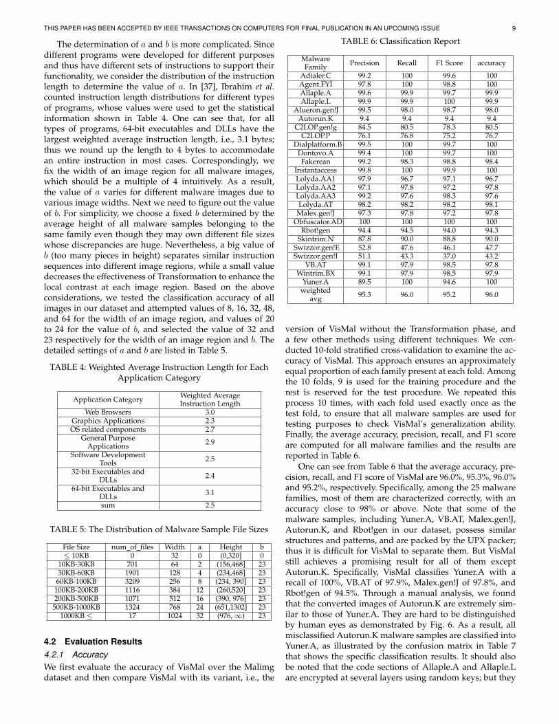
One can see from Table 6 that the average accuracy, pre-cision, recall, and F1 score of VisMal are 96.0%, 95.3%, 96.0%and 95.2%, respectively. Specifically, among the 25 malwarefamilies, most of them are characterized correctly, with anaccuracy close to 98% or above. Note that some of themalware samples, including Yuner.A, VB.AT, Malex.gen!J,Autorun.K, and Rbot!gen in our dataset, possess similarstructures and patterns, and are packed by the UPX packer;thus it is difficult for VisMal to separate them. But VisMalstill achieves a promising result for all of them exceptAutorun.K. Specifically, VisMal classifies Yuner.A with arecall of 100%, VB.AT of 97.9%, Malex.gen!J of 97.8%, andRbot!gen of 94.5%. Through a manual analysis, we foundthat the converted images of Autorun.K are extremely sim-ilar to those of Yuner.A. They are hard to be distinguishedby human eyes as demonstrated by Fig. 6. As a result, allmisclassified Autorun.K malware samples are classified intoYuner.A, as illustrated by the confusion matrix in Table 7that shows the specific classification results. It should alsobe noted that the code sections of Allaple.A and Allaple.Lare encrypted at several layers using random keys; but they


TABLE 7: Confusion Matrix

122 0 0 0 0 0 0 0 0 0 0 0 0 0 0 0 0 0 0 0 0 0 0 0 00 116 0 0 0 0 0 0 0 0 0 0 0 0 0 0 0 0 0 0 0 0 0 0 00 0 2947 0 0 0 0 0 0 0 2 0 0 0 0 0 0 0 0 1 0 0 0 0 01 0 0 1590 0 0 0 0 0 0 0 0 0 0 0 0 0 0 0 0 0 0 0 0 00 0 0 0 194 0 0 0 0 0 1 0 0 0 0 0 3 0 0 0 0 0 0 0 00 0 0 0 0 10 0 0 0 0 0 0 0 0 0 0 0 0 0 0 0 0 0 0 960 0 0 0 0 0 161 8 0 0 0 0 0 0 0 0 0 0 5 0 11 15 0 0 01 0 3 0 0 0 11 112 0 0 0 0 0 0 0 0 0 0 3 1 2 12 1 0 00 0 0 0 0 0 0 0 177 0 0 0 0 0 0 0 0 0 0 0 0 0 0 0 00 0 0 0 0 0 0 0 0 162 0 0 0 0 0 0 0 0 0 0 0 0 0 0 00 0 1 0 0 0 2 2 0 0 375 0 0 0 0 0 0 0 0 0 0 1 0 0 00 0 0 0 0 0 0 0 0 0 0 431 0 0 0 0 0 0 0 0 0 0 0 0 00 0 0 0 0 0 0 0 0 0 0 0 206 5 0 0 2 0 0 0 0 0 0 0 00 0 0 0 1 0 0 0 0 0 0 0 3 180 0 0 0 0 0 0 0 0 0 0 00 1 0 0 1 0 0 0 0 0 0 0 1 0 120 1 0 0 0 0 0 0 0 0 00 0 0 0 0 0 0 0 0 0 0 0 1 0 1 156 0 0 0 0 0 0 1 0 00 0 0 1 0 0 0 0 0 0 0 0 0 0 0 0 133 0 0 1 0 0 1 0 00 0 0 0 0 0 0 0 0 0 0 0 0 0 0 0 0 142 0 0 0 0 0 0 00 0 1 0 0 0 5 1 0 0 0 0 0 0 0 0 0 0 149 0 0 1 0 1 00 0 8 0 0 0 0 0 0 0 0 0 0 0 0 0 0 0 0 72 0 0 0 0 00 0 0 0 0 0 9 5 0 0 0 0 0 0 0 0 0 0 1 0 61 52 0 0 00 1 0 0 0 0 11 27 0 0 0 0 0 0 0 0 0 0 0 0 35 57 1 0 00 0 2 0 0 0 0 0 1 1 0 1 0 1 0 2 0 0 0 0 1 0 399 0 00 0 1 0 0 0 0 0 0 0 0 0 0 0 0 0 0 0 1 0 0 0 0 95 00 0 0 0 0 0 0 0 0 0 0 0 0 0 0 0 0 0 0 0 0 0 0 0 800

(a) Autorun.K sample1 (b) Autorun.K sample2

(c) Yuner.A sample1 (d) Yuner.A sample2

Fig. 6: Visual Similarity Example 1

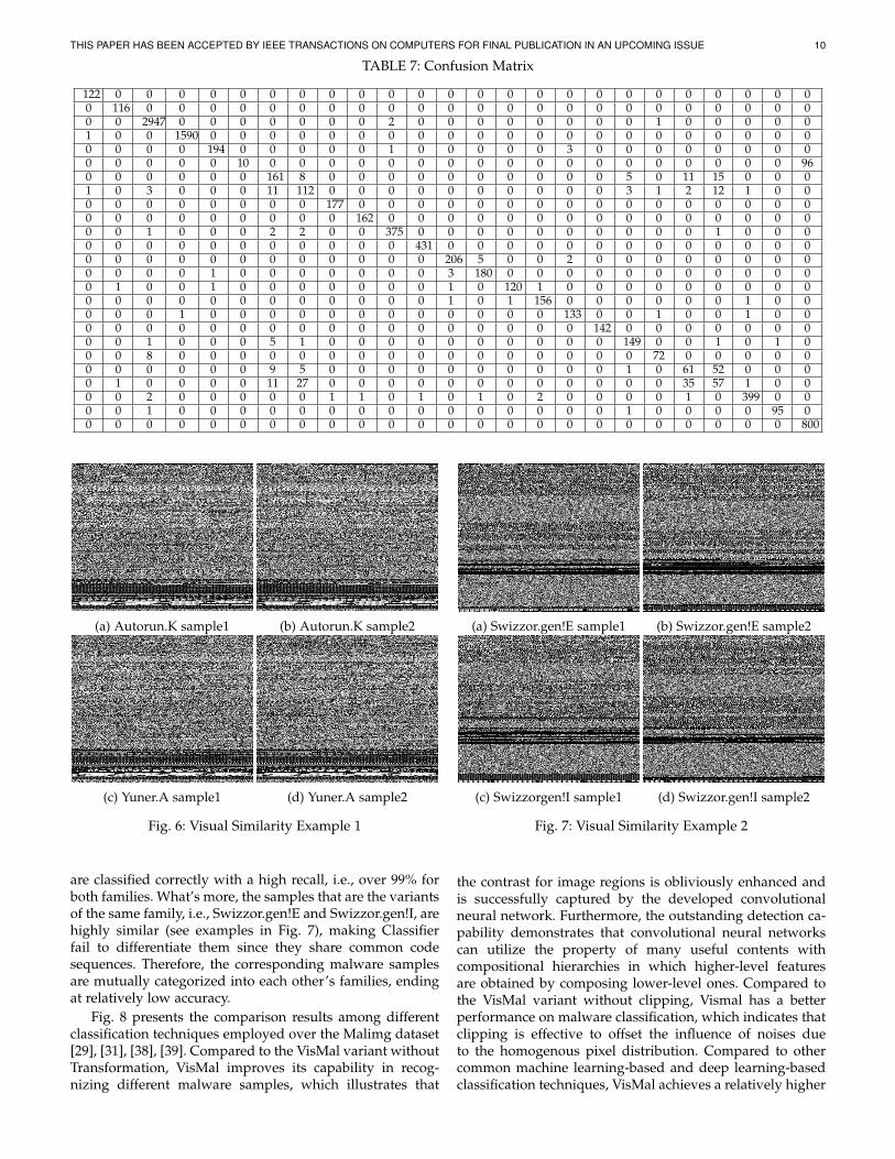
are classified correctly with a high recall, i.e., over 99% forboth families. What’s more, the samples that are the variantsof the same family, i.e., Swizzor.gen!E and Swizzor.gen!I, arehighly similar (see examples in Fig. 7), making Classifierfail to differentiate them since they share common codesequences. Therefore, the corresponding malware samplesare mutually categorized into each other’s families, endingat relatively low accuracy.

Fig. 8 presents the comparison results among differentclassification techniques employed over the Malimg dataset[29], [31], [38], [39]. Compared to the VisMal variant withoutTransformation, VisMal improves its capability in recog-nizing different malware samples, which illustrates that

(a) Swizzor.gen!E sample1 (b) Swizzor.gen!E sample2

(c) Swizzorgen!I sample1 (d) Swizzor.gen!I sample2


the contrast for image regions is obliviously enhanced andis successfully captured by the developed convolutionalneural network. Furthermore, the outstanding detection ca-pability demonstrates that convolutional neural networkscan utilize the property of many useful contents withcompositional hierarchies in which higher-level featuresare obtained by composing lower-level ones. Compared tothe VisMal variant without clipping, Vismal has a betterperformance on malware classification, which indicates thatclipping is effective to offset the influence of noises dueto the homogenous pixel distribution. Compared to othercommon machine learning-based and deep learning-basedclassification techniques, VisMal achieves a relatively higher


Classification Method Precision Recall F1 Score Accuracy

LR 60.6 96.4 74.4 67.4 NB 76.3 11.2 19.5 54.6

KNN 81.2 81.2 81.2 81.5 DT 85.9 85.6 85.7 86.0 AB 67.2 89.5 76.7 73.3 RF 89.9 88.6 89.2 89.5

SVM 70.0 84.4 76.5 74.5 DNN 90.6 91.1 90.9 91.0

MDMC 10.0 31.9 15.0 31.9 DRBA+CNN 94.6 94.5 94.5 94.5

GIST 97.7 97.7 97.7 97.7 VisMal without transformation 92.0 93.3 92.2 93.3

VisMal without clipping 92.0 92.7 91.5 92.7 VisMal 95.3 96.0 95.2 96.0

LR0

20

40

60

80

100

120

%

precision recall F1-score accuracy

NBKNN DT AB RF

SVMDNN

DRBA

+CNNVisMal

no_trans

VisMalMDMC

GISTVisMal

no_clip

Fig. 8: Accuracy of the Classification Methods

accuracy of 96.0%. To be specific, among the 7 commonmachine learning-based classification techniques and thedeep learning-based approach presented in [38], the deeplearning-based method demonstrates the best performancewith an accuracy of 91%, and LR achieves a very highrecall at a moderate accuracy because the classifier cate-gorizes a lot of malware samples from other families tothe rest of them. The CNN-based framework proposed in[39], namely DRBA+CNN, employs a BAT algorithm thatcan properly balance the number of samples in differentmalware families, achieving an accuracy of 94.5%. Besides,we reimplemented two malware image-based frameworks,namely GIST and MDMC that were respectively proposedin [29] and [31], where GIST utilizes the Gabor filters toextract statistical features for each malware gray image andcarefully selects 320 features as the input to the k-nearestneighbor algorithm for final classification, while MDMCconverts malware binaries into Markov probability matrixesby counting the frequency of two neighboring bytes andthen employs a deep convolutional neural network to cat-egorize different Markov probability matrixes. One can seethat although GIST performs slightly better than VisMal inaccuracy, its efficiency is far slower (described later). Onother other hand, VisMal significantly outperforms MDMCin malware classification.

TABLE 8: Efficiency of the Classification Methods

ExtractionTime

ClassificationTime

TotalTime

Nataraj et al. [29] 32.7 ms 2.1 ms 34.8 msCui et al. [39] – – 20 ms

Naeem et al. [40] – 4.27 s –Yuan et al. [31] 144.3 ms 191.5 ms 335.8 msVasan et al. [41] – – 1.18 sVerma et al. [30] 37 ms 10 ms 47 ms

VisMal 0.3 ms 3.7 ms 4.0 ms

4.2.2 EfficiencySince malware classification is a time-sensitive componentin any anti-virus product, and a small delay could missthe best opportunity to discover malware processes, theprocedure for distinguishing malware samples should takeshort time. We measured the CPU time of our datasetpassing through VisMal during the test procedure and cal-culated the average MPE per malware sample. To consider apractical setting for evaluating VisMal, we did not deploy iton servers or call GPUs. The efficiency evaluation resultsare reported in Table 8. One can see that VisMal incurs0.3 ms on feature extraction and 3.7 ms on classification,efficiently providing information to anti-virus products forfurther operations. Besides, we compared VisMal with thetechniques presented by the latest research ( [29] in 2011,[39] in 2018, [40] in 2019, [31] in 2020, [41] in 2020, and [30]in 2020) that mainly pay attention to efficiency on malware


classification over the same dataset. From Table 8 we noticethat VisMal takes the least extraction time and total time,and the second least classification time. Specifically, in termsof the time taken to extract features, VisMal is 108 timesfaster than the method proposed by Nataraj et al., and 122.33times faster than the method presented by Verma et al.Additionally, the classification time incurred by VisMal isreduced by 1153.05 times and 1.70 times compared with theapproaches in Naeem et al. and Verna et al., respectively. Be-sides the extraction time and classification time, a significantdecrease in total time (4 times) is reported for VisMal, whencompared to Cui et al., the second-fastest method reportedin Table 8.

4.2.3 VisualizationSince malware classification is an important componentintegrated into all anti-virus tools, its precision plays anessential role in making these tools effective. To analyze theperformance of VisMal, this section presents the visualiza-tion results in which malware samples are converted intoimages and then processed by the contrast-limited adaptivehistogram equalization algorithm. Visualization providesuseful information for manual analysis to ascertain whetherthe categorized malware samples are similar, which canhelp to confirm the performance of VisMal from a differentangle. As VisMal converts malware samples into images,it naturally offers security engineers a convenient way toanalyze malware samples and look for reasons when theyare misclassified, based on which security engineers canintegrate new techniques to improve the performance oftheir anti-virus products. Fig. 9 demonstrates the texturesimilarity among malware samples belonging to the samefamily and dissimilarity from those belonging to differentfamilies. As shown in 9a-9b, 9c-9d, 9e-9f, 9g-9h, 9i-9j, 9k-9l, one can see that each pair is almost indistinguishablein terms of their texture information since, in the samefamily, the samples share certain common instruction se-quences, and correspondingly their malware images tend tobe similar in certain regions. Conversely, malware samplesbelonging to different families, which are developed fordifferent purposes, make use of a dissimilar set of instruc-tion sequences and thus have a huge difference in pixels’distribution, see Figs. 9a and 9g as an example.

5 CONCLUSION AND FUTURE RESEARCH

In this paper, we propose a novel, efficient, and effectivesimple malware categorization framework titled VisMal,which can discover the underlying byte code similarity formalware samples that belong to a particular family. On onehand, VisMal alleviates the difficulty of security engineersto study the complicated structures of different malwaresamples based on static analysis, and in the meantime sig-nificantly improves the classifying efficiency from dynamicanalysis. On the other hand, VisMal focuses on texturerepresentation by converting malware samples into images,effectively subverting the traditional ways of understandingbinary information.

Note that VisMal pays attention to disclose the encodingart in byte codes and makes use of encoding to interpretthe similarity of malware samples belonging to the same

(a) Adialer.C sample1 (b) Adialer.C sample2

(c) Agent.FYI sample1 (d) Agent.FYI sample2

(e) Allaple.A sample1 (f) Allaple.A sample2

(g) Alueron.gen!J sample1 (h) Alueron.gen!J sample2

(i) Dialplatform.B sample1 (j) Dialplatform.B sample2

(k) Dontovo.A sample1 (l) Dontovo.A sample2



family and dissimilarity between different malware families.To improve the accuracy of classification, VisMal exploits acontrast-limited adaptive histogram equalization algorithmto increase the local contrast of each region for a malwareimage, and effectively transfers from looking for similarcodes to similar image regions. Moreover, VisMal providesa simple and convenient way for security engineers to vali-date the performance of classification and to further analyzethe factors confusing Classifier such that its performancecan be improved by adding new techniques into anti-virusproducts.

Our future research will be committed to finding outthe close relationship between the critical information ofmalware images learned by neural networks and the byte-code sequences, which may contribute to the extraction ofsignatures on behalf of a malware family. Such signaturescan be managed via blockchain technologies [42]–[44] tofacilitate malware detection by a broader audience. Weare also interested in the discovery of vulnerabilities inprograms by making use of visualization techniques, whichcould provide new insights to help developers improve theircodes for better classification performance. Besides, we willfurther strengthen our framework to distinguish malwareand benignware.

REFERENCES

[1] A. Pekta and T. Acarman, “Classification of malware familiesbased on runtime behaviors,” Journal of Information Security andApplications, vol. 37, pp. 91–100, 2017. [Online]. Available: https://www.sciencedirect.com/science/article/pii/S2214212617301643

[2] C. C. San, M. M. S. Thwin, and N. L. Htun, “Malicious softwarefamily classification using machine learning multi-class classi-fiers,” in Computational Science and Technology, R. Alfred, Y. Lim,A. A. A. Ibrahim, and P. Anthony, Eds. Singapore: SpringerSingapore, 2019, pp. 423–433.

[3] F. Zhong, X. Cheng, D. Yu, B. Gong, S. Song, and J. Yu, “Mal-fox: Camouflaged adversarial malwareexample generation basedon conv-gans againstblack-box detectors,” https://arxiv.org/pdf/2011.01509.pdf, 2020.

[4] A. Moser, C. Kruegel, and E. Kirda, “Limits of static analysisfor malware detection,” in Twenty-Third Annual Computer SecurityApplications Conference (ACSAC 2007), Miami Beach, FL, USA,2007, pp. 421–430.

[5] M. Y. Wong and D. Lie, “Intellidroid: A targeted input generatorfor the dynamic analysis of android malware,” in Network andDistributed System Security Symposium, 2015, pp. 1–15.

[6] A. Calleja, J. Tapiador, and J. Caballero, “The malsource dataset:Quantifying complexity and code reuse in malware develop-ment,” IEEE Transactions on Information Forensics and Security,vol. 14, no. 12, pp. 3175–3190, 2019.

[7] D. Korczynski and H. Yin, “Capturing malware propagations withcode injections and code-reuse attacks,” in Proceedings of the 2017ACM SIGSAC Conference on Computer and Communications Security(CCS’17), October 2017, pp. 1691–1708.

[8] N. Marastoni, A. Continella, D. Quarta, S. Zanero, and M. D.Preda, “Groupdroid: Automatically grouping mobile malware byextracting code similarities,” in Proceedings of the 7th SoftwareSecurity, Protection, and Reverse Engineering/Software Security andProtection Workshop (SSPREW-7), no. 1, December 2017, pp. 1–12.

[9] ——, “Andro-profiler: anti-malware system based on behaviorprofiling of mobile malware,” in Companion: Proceedings of the 23rdInternational Conference on World Wide Web, April 2014, pp. 737–738.

[10] J. Jiang, S. Li, M. Yu, G. Li, C. Liu, K. Chen, H. Liu, and W. Huang,“Android malware family classification based on sensitive opcodesequence,” in 2019 IEEE Symposium on Computers and Communica-tions (ISCC), 2019, pp. 1–7.

[11] F. Fasano, F. Martinelli, F. Mercaldo, and A. Santone, “Cascadelearning for mobile malware families detection through qualityand android metrics,” in 2019 International Joint Conference onNeural Networks (IJCNN), 2019, pp. 1–10.

[12] W. Blanc, L. G. Hashem, K. O. Elish, and M. J. Hussain Almohri,“Identifying android malware families using android-orientedmetrics,” in 2019 IEEE International Conference on Big Data (BigData), 2019, pp. 4708–4713.

[13] B. Jung, T. Kim, and E. G. Im, “Malware classification using bytesequence information,” in Proceedings of the 2018 Conference onResearch in Adaptive and Convergent Systems (RACS’18), 2018, pp.143–148.

[14] J. Saxe and K. Berlin, “Deep neural network based malware de-tection using two dimensional binary program features,” in 201510th International Conference on Malicious and Unwanted Software(MALWARE), 2015, pp. 11–20.

[15] A. Davis and M. Wolff, “Deep learning on disassembly data,”https://paper.seebug.org/papers/Security20Conf/Blackhat/2015/us-15-Davis-Deep-Learning-On-Disassembly.pdf, 2015.

[16] J. Kinable and O. Kostakis, “Malware classification based on callgraph clustering,” Journal in Computer Virology, vol. 7, pp. 233–245,2011. [Online]. Available: https://link.springer.com/article/10.1007/s11416-011-0151-yciteas

[17] O. Mirzaei, G. S. Tangil, J. M. de Fuentes, J. Tapiador, andG. Stringhini, “Andrensemble:leveraging api ensembles to char-acterize android malware families,” in Proceedings of the 2019 ACMAsia Conference on Computer and Communications Security (AisaCCS’19), 2019, pp. 307–314.

[18] M. Zhang, Y. Duan, H. Yin, and Z. Zhao, “Semantics-aware an-droid malware classification using weighted contextual api depen-dency graphs,” in Proceedings of the 2014 ACM SIGSAC Conferenceon Computer and Communications Security (CCS’14), November2014, pp. 1105–1116.

[19] K. Sethi, R. Kumar, L. Sethi, P. Bera, and P. K. Patra, “A novelmachine learning based malware detection and classificationframework,” in 2019 International Conference on Cyber Security andProtection of Digital Services (Cyber Security), 2019, pp. 1–4.

[20] A. Martin, V. Rodriguez-Fernandez, and D. Camacho,“Candyman: Classifying android malware families by modelingdynamic traces with markov chains,” Engineering Applicationsof Artificial Intelligence, vol. 74, pp. 121–133, 2018. [Online].Available: https://www.sciencedirect.com/science/article/abs/pii/S0952197618301374

[21] B. Anderson, D. Quist, J. Neil, C. Storlie, and T. Lane,“Graph-based malware detection using dynamic analysis,”Journal in Computer Virology, vol. 7, pp. 247–258, 2011.[Online]. Available: https://link.springer.com/article/10.1007/s11416-011-0152-xciteas

[22] G. E. Dahl, J. W. Stokes, L. Deng, and D. Yu, “Large-scale malwareclassification using random projections and neural networks,” in2013 IEEE International Conference on Acoustics, Speech and SignalProcessing, 2013, pp. 3422–3426.

[23] S. Tobiyama, Y. Yamaguchi, H. Shimada, T. Ikuse, and T. Yagi,“Malware detection with deep neural network using processbehavior,” in 2016 IEEE 40th Annual Computer Software and Ap-plications Conference (COMPSAC), vol. 2, 2016, pp. 577–582.

[24] Z. Zhang, P. Qi, and W. Wang, “Dynamic malware analysis withfeature engineering and feature learning,” in Proceedings of theAAAI Conference on Artificial Intelligence, vol. 34, no. 01, 2020, pp.1210–1217.

[25] D. Vij, V. Balachandran, T. Thomas, and R. Surendran, “Gramac:A graph based android malware classification mechanism,” inProceedings of the Tenth ACM Conference on Data and ApplicationSecurity and Privacy (CODASPY’20), 2020, pp. 156–158.

[26] Y. Park, D. Reeves, V. Mulukutla, and B. Sundaravel, “Fast mal-ware classification by automated behavioral graph matching,”in Proceedings of the Sixth Annual Workshop on Cyber Security andInformation Intelligence Research, 2010, pp. 1–4.

[27] S. Hsiao, Y. S. Sun, and M. C. Chen, “Behavior grouping ofandroid malware family,” in 2016 IEEE International Conference onCommunications (ICC), 2016, pp. 1–6.

[28] L. Nataraj, V. Yegneswaran, P. Porras, and J. Zhang, “A compar-ative assessment of malware classification using binary textureanalysis and dynamic analysis,” in Proceedings of the 4th ACMworkshop on Security and artificial intelligence (AISec’11), October2011, pp. 21–30.

[29] L. Nataraj, S. Karthikeyan, G. Jacob, and B. S. Manjunath, “Mal-ware images:visualization and automatic classification,” in Pro-ceedings of the 8th International Symposium on Visualization for CyberSecurity (VizSec’11), vol. 4, July 2011, pp. 1–7.

https://www.sciencedirect.com/science/article/pii/ S2214212617301643


https://arxiv.org/pdf/2011.01509.pdf

https://arxiv.org/pdf/2011.01509.pdf

https://paper.seebug.org/papers/Security20Conf/Blackhat/ 2015/us-15-Davis-Deep-Learning-On-Disassembly.pdf

https://paper.seebug.org/papers/Security20Conf/Blackhat/ 2015/us-15-Davis-Deep-Learning-On-Disassembly.pdf

https://link.springer.com/article/10.1007/s11416-011-0151-yciteas

https://link.springer.com/article/10.1007/s11416-011-0151-yciteas

https://www.sciencedirect.com/science/article/abs/ pii/S0952197618301374

https://www.sciencedirect.com/science/article/abs/ pii/S0952197618301374

https://link.springer.com/article/10.1007/s11416-011-0152-xciteas

https://link.springer.com/article/10.1007/s11416-011-0152-xciteas


[30] V. Verma, S. K. Muttoo, and V. Singh, “Multiclass malwareclassification via first- and second-order texture statistics,”Computers & Security, vol. 97, p. 101895, 2020. [Online].Available: https://www.sciencedirect.com/science/article/pii/S0167404820301681

[31] B. Yuan, J. Wang, D. Liu, W. Guo, P. Wu, and X. Bao,“Byte-level malware classification based on markov imagesand deep learning,” Computers & Security, vol. 92, p.101740, 2020. [Online]. Available: https://www.sciencedirect.com/science/article/pii/S0167404820300262

[32] D. Hargreaves, “Stratified k-fold: What it is &how to use it,” https://towardsdatascience.com/stratified-k-fold-what-it-is-how-to-use-it-cf3d107d3ea2, 2021.

[33] R. Dorothy, R. Joany, R. J. Rathish, S. S. Prabha, and S. rajendran,“Image enhancement by histogram equalization,” Int. J. Nano.Corr. Sci. Engg, vol. 2, no. 4, pp. 21–30, 2015.

[34] “Adaptive histogram equalization,” https://en.wikipedia.org/wiki/Adaptivehistogramequalizationcitenote-clahe87-3, 2021.

[35] K. Zuiderveld, “Contrast limited adaptive histogramequalization,” http://cas.xav.free.fr/Graphics%20Gems%204%20-%20Paul%20S.%20Heckbert.pdf, 1993.

[36] “Signal processing for malware analysis,” https://vision.ece.ucsb.edu/research/signal-processing-malware-analysis, 2021.

[37] A. H. Ibrahim, M. B. Abdelhalim, H. Hussein, and A. Fahmy, “Ananalysis of x86-64 instruction set for optimization of system soft-wares,” International Journal of Advanced Computer Science, vol. 1,no. 4, pp. 152–162, 2011.

[38] R. Vinayakumar, M. Alazab, K. P. Soman, P. Poornachandran, andS. Venkatraman, “Robust intelligent malware detection using deeplearning,” IEEE Access, vol. 7, pp. 46 717–46 738, 2019.

[39] Z. Cui, F. Xue, X. Cai, Y. Cao, G. Wang, and J. Chen, “Detection ofmalicious code variants based on deep learning,” IEEE Transactionson Industrial Informatics, vol. 14, no. 7, pp. 3187–3196, 2018.

[40] H. Naeem, B. Guo, M. R. Naeem, F. Ullah, H. Aldabbas, and M. S.Javed, “Identification of malicious code variants based on imagevisualization,” Computers & Electrical Engineering, vol. 76, pp.225–237, 2019. [Online]. Available: https://www.sciencedirect.com/science/article/pii/S004579061733776X

[41] D. Vasan, M. Alazab, S. Wassan, B. Safaei, and Q. Zheng,“Image-based malware classification using ensemble of cnnarchitectures (imcec),” Computers & Security, vol. 92, p.101748, 2020. [Online]. Available: https://www.sciencedirect.com/science/article/pii/S016740482030033X

[42] M. Xu, C. Liu, Y. Zou, F. Zhao, J. Yu, and X. Cheng, “wchain:A fast fault-tolerant blockchain protocol for multihopwirelessnetworks,” IEEE Transactions on Wireless Communication, 2021.[Online]. Available: https://arxiv.org/abs/2102.01333

[43] M. Xu, F. Zhao, Y. Zou, C. Liu, X. Cheng, and F. Dressler. Blown:A blockchain protocol for single-hop wireless networks underadversarial sinr. [Online]. Available: https://arxiv.org/abs/2103.08361

[44] M. Xu, S. Liu, D. Yu, X. Cheng, S. Guo, and J. Yu. Cloudchain:A cloud blockchain using shared memeory consensus and rdma.[Online]. Available: https://arxiv.org/abs/2106.04122





https://towardsdatascience.com/stratified-k-fold-what-it-is-how-to-use-it-cf3d107d3ea2

https://towardsdatascience.com/stratified-k-fold-what-it-is-how-to-use-it-cf3d107d3ea2

https://en.wikipedia.org/wiki/ Adaptivehistogramequalization citenote-clahe87-3

https://en.wikipedia.org/wiki/ Adaptivehistogramequalization citenote-clahe87-3

http://cas.xav.free.fr/Graphics%20Gems%204%20-%20Paul%20S.%20Heckbert.pdf

http://cas.xav.free.fr/Graphics%20Gems%204%20-%20Paul%20S.%20Heckbert.pdf

https://vision.ece.ucsb.edu/research/ signal-processing-malware-analysis

https://vision.ece.ucsb.edu/research/ signal-processing-malware-analysis

https://www.sciencedirect.com/science/article/pii/ S004579061733776X




https://arxiv.org/abs/2102.01333




Documents

IEEE TRANSACTIONS ON COMPUTERS 1 Malware-on-the-Brain