IEEE SENSORS JOURNAL, VOL. 9, NO. 5, MAY 2009 515

IEEE SENSORS JOURNAL, VOL. 9, NO. 5, MAY 2009 515

Calibration-Free Measurement of Liquid Permittivityand Conductivity Using Electrochemical Impedance

Test Cell With ServomechanicallyAdjustable Cell Constant

Hongshen Ma, Member, IEEE, Jeffrey H. Lang, Fellow, IEEE, and Alexander H. Slocum

Abstract—This paper presents a technique and a device formeasuring the permittivity and conductivity of liquids and gasesthat does not require prior calibration by a reference sample.The technique involves precisely controlling the separation be-tween two closely spaced spherical electrodes to make electricalimpedance measurements of the sample media as a function ofelectrode separation. By leveraging the geometrical accuracy ofthe spheres and precise control of the electrode separation, thepermittivity and conductivity of the sample can be extracted usinga simple geometrical model of the electrode. Calibration usinga reference sample is replaced by mechanical calibration of thesphere diameter and separation control mechanism, which canbe engineered simply and accurately using standard componentsand processes. The electrode separation is adjusted using a flexurestage and a servomechanical actuator, which enables control ofthe electrode separation with 0.25 nm resolution with a 50 �

range. Permittivity and conductivity measurements within 1% ofestablished values have been demonstrated.

Index Terms—Calibration-free measurements, conductivity,electrochemical impedance, permittivity, water purity.

I. INTRODUCTION

E LECTRICAL permittivity and conductivity are fun-damental physicochemical properties of liquids. In

solutions, permittivity is a measure of the polarizability of thesolvent, while conductivity is a measure of the concentrationand mobility of the solute. Applications of permittivity mea-surements include determining the composition of solvents insolution chemistry [1], [2], soil moisture content in geologicalsurvey [3], and liquid-gas fraction in chemical processing

Manuscript received June 08, 2008; revised September 02, 2008; acceptedSeptember 05, 2008. Current version published March 27, 2009. This researchwas supported in part by MIT’s Center for Bits and Atoms under NSF GrantCCR-0122419). An earlier version of this paper was presented at the 2007 IEEESensors Conference and was published in its proceedings. Any opinions, find-ings, and conclusions or recommendations expressed in this paper are those ofthe authors and do not necessarily reflect the views of the NSF. The associateeditor coordinating the review of this paper and approving it for publication wasProf. Evgenty Katz.

H. Ma and A. H. Slocum are with the Department of Mechanical Engineering,Massachusetts Institute of Technology, Cambridge, MA 02139 USA (e-mail:[email protected]; [email protected]).

J. H. Lang is with the Department of Electrical Engineering and ComputerScience, Massachusetts Institute of Technology, Cambridge, MA 02139 USA(e-mail: [email protected]).

Color versions of one or more of the figures in this paper are available onlineat http://ieeexplore.ieee.org.

Digital Object Identifier 10.1109/JSEN.2009.2015401

[4], [5]. Applications of conductivity measurements includedetermining contaminant levels in drinking water, boiler waterpurity in power plants [6], health of lubrication oils in heavymachinery [7], performance of battery electrolyte [8], and con-centration of chemical products in microfludic analysis systems[9]. Electrical conductivity of liquids can also be used to detectthe presence of specific chemicals if coupled with enzymaticassays designed to produce conductiometric readout [10].

Accurate and repeatable permittivity and conductivity mea-surements are key requirements of sensor systems that utilizethis mode of detection. Since permittivity and conductivity,and , are intensive parameters, they must be derived from themeasurable quantities of capacitance and conductance, and

, using a geometrical model of the impedance test cell de-scribed by the cell constant, . These quantities are relatedby the following equations:

(0.1)

(0.2)

where the capacitance and conductance , are parasiticvalues not included in the model for .

While the values of capacitance and conductance can be mea-sured with a high degree of accuracy, the variability of , ,and can result in inaccuracies in and . Since anddepend on the detailed geometry of the electrodes and their man-ufacturing process, the values of these terms cannot be easilypredicted. As a result, determining and based on a geomet-rical model of is extremely difficult. The addition of guardelectrodes can reduce the value of and , but not eliminatethem completely. Surface properties such as electrode polariza-tion [11], corrosion, and absorption, can produce additional er-rors by altering the size of the impedance test cell. In portableand/or low-cost analysis systems with limited sample volume,the effect of these aforementioned errors may be further exag-gerated, thus nullifying the use of these systems to measureand .

Existing conductivity meters typically address the uncertaintyof by periodically calibrating the impedance test cell usinga standard solution with established values of and . This cor-rection is of limited value since , and can also bedependent on the value of and . As a result, the calibration

1530-437X/$25.00 © 2009 IEEE

Authorized licensed use limited to: The University of British Columbia Library. Downloaded on March 14,2010 at 20:48:24 EDT from IEEE Xplore. Restrictions apply.

516 IEEE SENSORS JOURNAL, VOL. 9, NO. 5, MAY 2009

is valid only when and of the sample and calibration fluidare within a narrow range of one another [7], [8]. The use ofcalibration liquids is also often impractical since the calibrationliquid may irreversibly contaminate the impedance test cell.

Accurate measurement of permittivity and conductivitywithout wet calibration can be made using impedance test cellswhere the cell constant can be adjusted in a predictable manner.A variable cell constant could be implemented by either ad-justing the separation between the electrodes or the electrodeoverlap area. The former technique have been used by Barthel[12], [13] and by Wu [14] to obtain standard reference valuesfor permittivity and conductivity [15], [16]. These devicesencapsulate sample media in a glass cylinder with platinumelectrodes mounted on the end of the cylinder. The cylindercontains a removable section of a precisely measured length.The differential capacitance and conductance measured withand without the middle section is used to compute the absolutepermittivity and conductivity.

A simpler method for adjusting the cell constant was devel-oped by Shiefelbein [8], which consists of an inner rod elec-trode concentric with an outer cylindrical electrode. By varyingthe level of immersion of the electrode in the sample media, theabsolute value of permittivity and conductivity can be extractedfrom the differential values of capacitance and resistance. Usingthis apparatus, Shiefelbein demonstrated that the conductivity ofKCl solutions could be measured to within 1% of standard ref-erence values.

The design of impedance test cells with an adjustable cellconstant highlights a fundamental tradeoff between varying thecell constant over a range sufficient to make an accurate esti-mate of the permittivity and conductivity, while minimizing thevariation of parasitic capacitance and conductance. This tradeoffcan be optimized at small electrode separations because smallmodulations of the electrode separation result in large variationsof the cell constant, while the corresponding variations of para-sitic capacitance and conductance are minimized. In the devel-opment of portable chemical analysis systems, where a conduc-tivity assay may be used to detect the presence of target chem-icals, small gap electrode geometries are also advantageous forreducing the volume of reactants, and correspondingly, the totalcost of analysis.

The design of impedance test cells with small, adjustableelectrode separations between planar electrodes has many prac-tical challenges since parallelism errors between the electrodescan produce large offsets in the measured result. The designfor such apparatuses for permittivity and conductivity measure-ments has been explored without success using the apparatusof White [17] and the apparatus of Wu [18]. The parallelismproblem can be avoided using spherical electrodes since thenearest points between two spheres are by definition tangential.(This principle is similarly true for the geometry of a sphereand a plane.) Additionally, spheres can be inexpensively manu-factured with high diametrical accuracy and extremely smoothsurfaces. For polished spheres that are a few millimeters in di-ameter, the diametrical tolerance can typically be less than onemicrometer, while the RMS surface roughness can be as low asa few nanometers.

Fig. 1. Electrostatic model.

The technique presented in this paper leverages the diamet-rical tolerance of a sphere and precise adjustment of the elec-trode separation to enable accurate measurement of permittivityand conductivity. The wet calibration required in previous de-vices is replaced by mechanical calibration of the sphere di-ameter and separation control mechanism, which can be engi-neered simply and accurately using standard components andprocesses. The concept for this device and its demonstrationon permittivity measurements has been described in an earlierpublication [19]. This paper describes the detailed design of thedevice and demonstrates its use for conductivity measurements[20].

II. THEORY

A. Electrostatic Model

The capacitance between two perfectly conductingspheres, in a uniformally polarizable media, shown in Fig. 1,has the exact expression [21]

(1.1)

(1.2)

where is the radius of the spheres, is the vacuum permit-tivity, is the relative permittivity, and is the distance be-tween the electrodes measured from their nearest points. Whenthe two electrodes are extremely close to one another, i.e.,

, the following approximate expression:

(1.3)

derived by Boyer [21], could be used, where is a constant.This expression has the characteristic that the spatial derivativeof is inversely proportional to such that

(1.4)

Thus, using the capacitance measured at several values of , it istherefore possible to extract the value of . Furthermore, sincethe physical laws governing conductance are exactly parallel to


MA et al.: CALIBRATION-FREE MEASUREMENT OF LIQUID PERMITTIVITY AND CONDUCTIVITY 517

Fig. 2. Equivalent circuit representations of: (a) uniformally polarizable mediaand (b) media with mobile charge carriers.

capacitance, the relationship between conductance and conduc-tivity obey the expression

(1.5)

which correspondingly gives

(1.6)

B. Electrochemical Model

Uniformally polarizable media without mobile charge car-riers such as air and hexane can be modeled using a simpleequivalent circuit consisting of a capacitor , and a resistor

in parallel, as shown in Fig. 2(a). Sample media with mobilecharges, such as water and alcohols form an electrical doublelayer at the electrode-electrolyte interface. The electrical prop-erties of the double layer in the non-faradic regime can be ap-proximately described using the Gouy–Chapmann–Stern (GCS)model [22]. While the validity of this model has recently beencalled into question [23], for the purpose of measuring proper-ties of the bulk liquid independent of surface layer effects, it issufficient to approximate this region using the equivalent circuitmodel shown in Fig. 2(b). The effect of the double layers onboth electrodes is represented using the series circuit elements

and . Physically, represents the buildup of charge inthe double layer, while represents conductivity of the inter-facial region resulting from this accumulation of charge. Thelack of a DC conductance path in this model is an artifact of ablocking, or nonreactive, electrode that does not permit direct

Fig. 3. Bode plot of the equivalent circuit of an impedance cell containing mo-bile charge carriers.

transport of electrons from the electrode and the solution. Theimpedance of the circuit in Fig. 2(b) is

(1.7)

Combining the terms into one fraction (1.7), becomes

(1.8)which can be expressed as

(1.9)

Equation (1.9) has a pole at the origin, a second pole at ahigher frequency, and two zeros. A Bode plot of the impedanceis shown in Fig. 3. The pole at the origin arises from the ca-pacitor , while the second pole arises from the time constantof the bulk liquid defined by the elements, and . The fre-quency of this pole is intrinsic to the sample media since

(1.10)

Thus, in order to obtain precise measurements of and in thefrequency domain, it is important to excite the system near thisfrequency. For aqueous solutions at room temperature, the valueof is expected to be approximately , while the value ofis expected to range between and 0.1 S/m. The fre-quency of will therefore range from approximately 220 Hzto 22 MHz.

The expression for the zeros of (1.9), and , can bedetermined to be (1.11) shown at the bottom of the page. Anapproximate expression for the lower frequency zero, , as

(1.11)



a function of its dominant terms can be obtained by rewriting(1.11) as

(1.12)

where

(1.13)

(1.14)

Expression (1.11) can be rewritten again as the series expansion

(1.15)

where

(1.16)

Taking the first two terms of the series yields an approximateexpression for

(1.17)

This expression is a rather intuitive result, which says that thevalue of is determined by the time constant of the bulkimpedance, the time constant of the interfacial impedance, andthe time constant that describes the interaction between thesetwo components. Expressions (1.10) and (1.17) indicate that thefrequency of is lower than that of and thus validatingthe Bode plot in Fig. 3.

An approximate expression can also be derived for the higherfrequency zero, . Since it can be shown that

(1.18)

the second term under the square root in (1.11) can effectivelybe neglected. The expression for can thus be approximatedas

(1.19)

The expressions for and can be further simplifiedby comparing the terms of . Since theelectrode separation is generally much greater than the effec-tive length of the interfacial layer, which is characterized by theDebye length and is typically no more than 100 nm, it can beassumed that and . Therefore, it can be as-sumed and . Asa result, the expressions for and can be written as

(1.20)

(1.21)

Reapplying the previous argument yield the results

(1.22)

It should be noted, however, that in situations where the elec-trode separation is less than or approximately equal to the Debyelength, these assumptions no longer hold, and more sophisti-cated models are required to interpret the measured impedance.

III. DEVICE DESIGN

A. Electrode

The spherical electrodes are fabricated using silicon-nitridespheres as the substrate for a thin platinum film. Traditionallyused in low-friction bearings and precision alignment equip-ment, silicon-nitride spheres have exceptional dimensional ac-curacy, mechanical stiffness, surface quality, and stability overtemperature.

The spheres used to fabricate the electrode have a diameter of9.5252 mm with a tolerance of (Cerbec Saint GobainCeramics: Grade 5 spheres). The surface quality of the sphereshas been analyzed using a whitelight profilometer (Zygo), whichshowed a surface roughness of 2 nm RMS and the peak-to-valleyrange of approximately 50 nm. For comparison, polished siliconwafers analyzed using the same instrument showed a surfaceroughness of 1 nm RMS and a peak-to-valley range of 20 nm.

The electrode film consists of a 50 nm platinum layer and a5 nm chromium adhesion layer. The metal films are depositedon one hemisphere of the silicon-nitride spheres using elec-tron-beam deposition. Further surface analysis confirmed thatthe electrode films coat the silicon-nitride spheres conformallyand does not change its surface roughness characteristics.

As Section V will show, while this choice of electrodematerials is sufficient for permittivity measurements, the cor-responding conductivity measurement showed a slow increaseover time, which is likely caused by dissimilar metal contactsbetween the sphere and its mechanical mount. This problemhas been resolved using ANSI-316 stainless-steel spheres tomatch the metal used to fabricate the mounting structure for theelectrode.

B. Impedance Test Cell

The electrodes are mechanically constrained in a cylindricalbore on the tip of a 12.7 mm diameter, ANSI-316 stainless-steelshaft. An externally threaded ring nut constrains the electrodesphere inside the bore with only a small region protruding, asshown in Fig. 4. Two dimples on the ring nut allow it to be tight-ened using a custom-made wrench. When tightened, the ring nutbends slightly and applies a mechanical preload to the electrodeto ensure that the electrode and shaft are tightly bound together.Mechanical contact between the ring nut and the electrode alsoserves as the electrical contact between the platinum film andthe mounting shaft. Therefore, the mounting shaft becomes partof the electrode for measuring impedance. The addition of theelectrode mounting structure introduces an error to the shapeof the electrodes. However, since most of the electric energy isconcentrated in the small gap region between the electrodes, theeffect of this error is minimal if measurements are made at smallelectrode gaps.

The electrode separation is modulated by precise adjustmentof the position of the mounting shafts using a flexural stage.



Fig. 4. Cross section of the electrode mount and the sample chamber.

The two mounting shafts are aligned in the flexure mechanism,but are electrically isolated from the mechanism via a 50layer of polyimide film (McMaster: 2271K72). The displace-ments of both mounting shafts are measured using capacitanceprobes (Lion precision) pointed at the end of the shaft as shownin Fig. 5. Grounded target electrodes epoxied to the end of eachshaft prevent the capacitance probe from interfering with theimpedance measurement.

The sample chamber is designed to constrain the samplefluid between the electrodes while allowing small modulationsof the electrode separation. As shown in Figs. 4 and 7, thesample chamber is approximately a cube with a central borefor the mounting shafts. The sample chamber is fabricatedusing ANSI-316 stainless steel with external dimensions of

. A liquid seal is establishedbetween each mounting shaft and the sample chamber via aKalrez O-ring ( 206 Dupont compound 4079), which hasproperties similar to Teflon, but with significantly greaterelasticity.

It is important to note that when the electrode separation is ad-justed over the designed range of 50 , the O-ring does not slipagainst the mounting shaft or the O-ring grooves in the samplechamber. Rather, the O-rings act as elastic elements (flexures)that enable this deflection by shear strain. As a result, the mo-tion of the shaft is mechanically repeatable and does not sufferfrom hysteric errors inherent in sliding contacts.

Liquid samples are introduced into the sample chamber viafluidic ports for 1/16-inch OD tubing (Upchurch: M-644-03),connected to a standard syringe. The inlet port is located nearthe bottom of the chamber while the outlet port is located nearthe top in order to prevent air bubbles from accumulating inthe chamber. The chamber also contains a window for debug-ging purposes. This window is covered with a 3-mm-thick roundPyrex window (Esco products: P705125), which is also sealedusing a Kalrez O-ring.

C. Positioning Mechanism

The positioning mechanism, shown in Fig. 6, is a 6061 T651aluminum monolith consisting of three main functional groups:coarse adjustor; fine adjustor; and metrology frame. The elec-trode mounting shafts are constrained to the aluminum monolith

using a semicircular clamp, as shown in Fig. 7. The top shaft isconnected with a symmetric dual beam flexure, which is partof the fine actuator. The bottom shaft is not rigidly clampedwhen the coarse adjustor is active, but once the desired positionhas been reached, this shaft is similarly fixed via a semicircularclamp.

The coarse adjustor sets the initial separation of the elec-trodes to within range of the fine adjustor. This mechanismconsists of an ultra fine thread lead screw (Thorlabs: 1/4 -80screw FS25AB200), shown in Fig. 7, that advances the bottommounting shaft. The positioning accuracy is enhanced by ananti-backlash bushing which applies a consistent preload to thescrew. Assuming 1 angular resolution is achievable by hand,the position of the electrode can be advanced with a resolutionof 0.3 . In order to prevent the lead screw from deformingthe flat surface, a steel puck with one flat and one conical sur-face is added to the interface between the spherical tip on thelead screw and the flat surface of the mounting shaft.

The coarse adjustor is mounted on a separate aluminum blockthat can be detached from the main frame. Once the desiredelectrode position has been reached, the bottom mounting shaftcan be rigidly clamped to the frame. The coarse adjustor canthen retracted and replaced by a capacitance probe that measuresthe displacement of the bottom mounting shaft. The removablecoarse adjustor reduces the complexity of having to measure anddeflect the same surface.

The fine adjustor is designed to control the position of thetop electrode mounting shaft with nanometer accuracy from aservomechanical actuator. There are four main components inthis mechanism: symmetric dual beam flexure, wobble pin, can-tilever beam, and the linear servo actuator.

The symmetric dual beam flexure constrains the displacementof the top shaft along the vertical direction with high mechan-ical impedance. The ratio of the stiffness of this flexure relativeto that of the cantilever beam acts to demagnify the displace-ment of the actuator with a high transmission ratio. The stiff-ness of this flexure is controlled by the length and width of theflexure beams. These dimensions are chosen to maintain max-imum stiffness, while staying within the load capabilities of theactuator.

A common problem in high transmission ratio flexure mecha-nisms is the presence of parasitic displacement along orthogonalaxes. In order to constrain displacement of the top shaft alongthe axis, while reducing parasitic displacement along theand axes, a wobble pin is used to transfer displacement fromthe cantilever beam to the symmetric dual beam flexure. Insteadof a standalone pin assembled between the transducer and theend-effector to only transmit axial forces [24], the wobble pinused here is monolithic with the rest of the flexure and consistsof two thin flexure beams. The two-prong design provides theflexibility desired in a wobble pin with the capability of inte-grating a capacitance probe through its center. The two-prongflexure beams are manufactured by first drilling a center hole inthe flat aluminum stock, and removing a small amount of ma-terial away from the exterior faces, before using a Waterjet Ma-chining Center (OMax) to make the final cut.

The cantilever beam reduces the displacement from the ac-tuator to the symmetric dual beam flexure. A tapered single-beam design efficiently distributes stress along the length of thebeam. The transmission ratio is set by the relative stiffness of the



Fig. 5. Design of the impedance cell.

Fig. 6. The mechanism for adjusting the electrode separation.

symmetric dual beam flexure and the stiffness of the cantileverbeam. These values are optimized using finite element analysisto set a transmission ratio of 200:1. The maximum deflectionof the cantilever beam is designed to be 50% of the yield stressof 6061-T6 aluminum, which limits maximum deflection to beapproximately 10 mm, corresponding to a maximum range of50 . The range of the flexure is enforced using mechanicalstops built into the structure of the flexure.

A linear actuator advances the electrode position by de-flecting the tip of the cantilever beam. This actuator is aservomechanical leadscrew with feedback from an optical ro-tary encoder (Newport: LTA-HL). This actuator has a minimumincremental step of 50 nm and a 7 nm encoder resolution. Basedon the designed 200:1 transmission ratio, this mechanism canbe positioned in increments of 0.25 nm. The tip of the actuatoris a nonrotating sphere, 6 mm in diameter. In order to ensureconsistent contact between the actuator and the cantileverbeam and prevent plastic deformation of the beam, a polishedtungsten-carbide flat is added to the interface between the tipof actuator and the tip of the cantilever beam. The polishedtungsten-carbide flat is found from a triangular lathe insert, andit is epoxied to the tip of the cantilever beam.

The displacements of both electrode mounting shafts aremeasured using capacitance probes (Lion Precision), as shown

Fig. 7. Close up of the adjustment mechanism.

in Fig. 5. Grounded target electrodes are epoxied to the endof each electrode shaft in order to prevent the capacitanceprobe from interfering with the impedance measurement. Theaccuracy of these capacitance probes are specified with an RMSresolution of 0.2 nm at a bandwidth of 100 Hz. These probes aremounted in a metrology frame that is structurally isolated fromthe rest of the mechanism. The metrology frame is C-shaped, asopposed to an ideal closed shape. However, this is compensatedby its robust size and integration with the aluminum monolithfrom which the entire device is constructed. The top probereaches through a hole between the two flexures of the wobblepin. The diameter of the hole is greater than the diameter of



the probe in order to prevent the motion of the cantilever beamfrom displacing the probe. The sum of the readout from thecapacitance probes gives a precise measurement of the changein the electrode separation. The two probe setup accounts forpossible errors caused by the finite stiffness of the flexure frameand the connection between the electrode shaft and the frame.

D. Impedance Measurement

The interelectrode sample impedance is measured usingan Agilent 4284A LCR meter, which uses an auto-balancingbridge circuit [25] to measure the complex impedance witha high degree of accuracy. This measurement configurationhas the advantage that one measurement terminal is held ata virtual ground, which means that guard electrodes used toreduce the amount of stray impedance can simply be connectedto the ground of the 4284A. For the apparatus described in thispaper, both the sample chamber and the flexure mechanism areconnected to ground to act as guard electrodes.

E. Data Acquisition and Temperature Control

Data acquired from the 4284A and the capacitive displace-ment probes are digitized and transmitted via GPIB to a PCwhere a Visual Basic program collects and stores the data. Theentire apparatus is enclosed within a temperature-controlledchamber. The temperature inside the chamber is modulatedusing a radiator system fed by a circulating refrigerator(NESLab RTE). The temperature value could be adjustedwithin C from the ambient temperature.

IV. ANALYSIS

An important property of this device is that the absolute elec-trode separation, , cannot be measured directly. Instead, ca-pacitance probes measure displacement along the axis, whichmeans that the value of is known to within an offset suchthat . The output value consists of ordered pairs ofimpedance values as a function of . In the frequency range out-lined in the electrochemical model of the system, the measuredimpedance could be separated into corresponding values ofand which correspond to and (the reciprocal of ).The value of and can be extracted using the spatial deriva-tives of and , according to (1.4) and (1.6). Since data pointsare collected as discrete values, the value of the derivative canbe estimated using the secant approximation where

(3.1)

The Value of is evaluated at the midpoint of and, and using the derivation for permittivity as an example,

(1.4) becomes

(3.2)

At this point, it is convenient to define a new variables andsuch that

(3.3)

and

(3.4)

The permittivity can therefore be determined by a linear leastsquares fit of the ordered pairs of to . As aresult,

(3.5)

One of the underlying assumptions of least squares fitting isthat the standard deviation of the variables is constant for allvalues. This assumption is violated for , since is a functionof the differential values of and . At large electrodes sepa-rations, is relatively small, and this means that the standarddeviation of , or is relatively large. At small electrodeseparations, the converse is true. Effects of the variable canbe compensated using a weighted least squares (WLS) fitting. Inthe standard application of this technique, the weight function,

, is defined as the reciprocal of the variance of the data

(3.6)

Assuming that the effect of the uncertainty in is muchgreater than the uncertainty of , the weight function can bederived using standard statistical formulae as

(3.7)

Since the value of is initially unknown, an initial guess forcan be obtained using a simple least squares fit. Estimates

for can then be improved using iterative application of theWLS fitting procedure. Three iterations are typically sufficientfor to converge to within 1 nm. The values for and canalternatively be extracted using direct nonlinear fitting to (1.3)and (1.5). However, these studies are less robust to noise thanweighted least squares.

V. RESULTS AND DISCUSSIONS

A. Electrical Permittivity Measurements

The operation of this device is initially characterized usingdry nitrogen gas, which has a permittivity of 1.00 and negligibleconductivity. These measurements are made starting at a largeelectrode gap, typically 10–15 , and decremented in stepsof approximately 0.5 until the electrodes come into contactwith one another. The sinusoidal excitation signal has an ampli-tude of 500 mV RMS, and a frequency of 120 kHz; 120 kHz ischosen because it is least affected by nearby electronic interfer-ence sources, such as the PWM signal from the servomechanicalactuator.

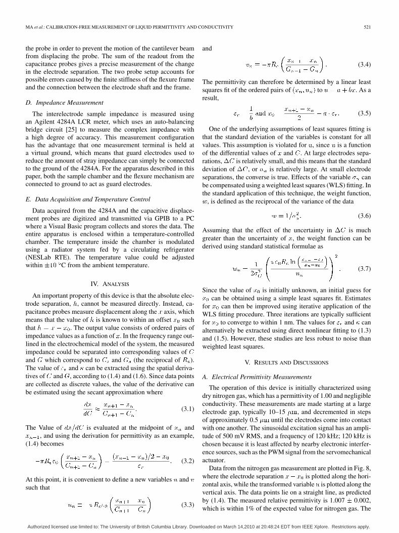
Data from the nitrogen gas measurement are plotted in Fig. 8,where the electrode separation is plotted along the hori-zontal axis, while the transformed variable is plotted along thevertical axis. The data points lie on a straight line, as predictedby (1.4). The measured relative permittivity is 1.007 0.002,which is within 1% of the expected value for nitrogen gas. The



Fig. 8. Permittivity results for nitrogen gas transformed according to (3.3).

Fig. 9. The permittivity of methanol, isopropanol, and 0.1 mM KCl solution.

positive offset between the measured and the known value isa result of the presence of the electrode mounting shaft, whichcauses data points from larger electrode separations to droopdownward in Fig. 8. This droop enlarges the measured permit-tivity by approximately 1% in the 1–10 electrode separationrange.

Measured data for isopropanol, methanol, and water areplotted together in Fig. 9. A 0.1 mM KCl solution is usedinstead of deionized water in order to control the concentrationof impurities at a stable level. The measurement parameters areexactly the same as nitrogen gas with the exception that theexcitation amplitude is decreased to 10 mV RMS in order toprevent faradic reactions at the surface of the electrode. Themeasured data in these plots show significantly less noise thanthe data for nitrogen gas due to the higher permittivity valuesof these fluids. The measured for isopropanol at 17.5 C,methanol at 17.8 C, and a 0.1 mM KCl solution at 22.2 Care 20.50 0.06, 33.80 0.06, and 79.74 0.13 respectively.The established values for these substances at the specifiedtemperatures are 20.62, 34.06, and 79.26 [15].

Fig. 10. Example data from conductivity of KCl solutions.

The repeatability of permittivity measurements has beenstudied using 30 repeated measurements of methanol at17.7 C. The mean of the measured is 34.5 with a standarddeviation of 0.09. Once again, the measured values are approx-imately 1% greater than the known of 34.1 for methanol at17.7 C.

B. Electrical Conductivity Measurements

With each dataset, electrical conductivity data is collected si-multaneously the electrical permittivity data. An example dataset from electrical conductivity measurements of a 10 mM KClsolution is shown in Fig. 10. The measurements are made at800 kHz, near the maximum frequency of the 4284A, while allother experimental conditions are identical to the permittivitymeasurements in Fig. 9. The conductivity results show morenoise than the permittivity measurement because the measure-ment frequency is no longer the optimal measurement frequencydescribed by the electrochemical model.

The conductivity of most solutions is approximately propor-tional to the molarity of ions in the solution. Therefore, con-ductivity measurements are more conveniently described usingmolar conductivity, , defined as the electrical conductivity nor-malized over concentration as

(4.1)

The variation of molar conductivities of KCl solutions can bepredicted from Fuoss–Onsager theory [12] using

(4.2)

where , , , , are constants that must be measured tohigh accuracy by Barthel [12].

The molar conductivity of KCl solutions as a function ofKCl molarity is shown in Fig. 11. Each data point representsthe mean of approximately ten data sets, while the error barsindicate the standard deviation of that data set. The spread ofthe measured data largely fall within 1% of the establishedvalue. Measurements using platinum electrodes showed a slow



Fig. 11. Measured versus established molar conductivity of KCl solutions from0.1 to 10 mM.

upward drift in the measured conductivity as a function of time.This drift error can be eliminated using ANSI-316 stainless steelspherical electrodes in place of the platinum electrodes. This be-havior indicates that the slow increase in conductivity is causedby galvanic potentials established by platinum-stainless steeljunction, which may oxidize the electrode and released free ionsinto the solution. While stainless steel electrodes provide suffi-cient diametrical accuracy for simple measurements, if the lowsurface roughness of silicon-nitride spheres is desired, the gal-vanic potential problem may be resolved by plating the elec-trode mounting shaft with a metal compatible with the metaldeposited on the silicon-nitride spheres.

VI. CONCLUSION

A technique and device for measuring the bulk electricalpermittivity and conductivity of liquids and gases withoutrequiring prior calibration has been developed. The capabilityof this technique to measure electrical permittivity withoutrequiring adjustment to the measurement apparatus or dataanalysis techniques was verified by measuring nitrogen gas,methanol, isopropanol, and water. The capability of this tech-nique for measuring electrical conductivity was verified bymeasuring the conductivity of aqueous KCl solutions from mMto 10 mM. Results were primarily within 1% of establishedvalues were obtained without adjustment of the apparatus ordata analysis techniques.

ACKNOWLEDGMENT

The authors wish to thank D. R. Sadoway and A. J.Grodzinsky for insightful discussions, and K. Broderick andM. Belanger for assistance with design and fabrication.

REFERENCES

[1] M. Tjahjono, T. Davis, and M. Garland, “Three-terminal capacitancecell for stopped-flow measurements of very dilute solutions,” Rev. Sci-entific Instrum., vol. 78, p. 023902, Feb. 2007.

[2] F. A. Wang, W. C. Wang, Y. L. Jiang, J. Q. Zhu, and J. C. Song, “A newmodel of dielectric constant for binary solutions,” Chem. Eng. Technol.,vol. 23, pp. 623–627, Jul. 2000.

[3] M. Bittelli, M. Flury, and K. Roth, “Use of dielectric spectroscopy toestimate ice content in frozen porous media,” Water Resources Res.,vol. 40, p. W04212, Apr. 22, 2004.

[4] W. Warsito and L. S. Fan, “Measurement of real-time flow structuresin gas-liquid and gas-liquid-solid flow systems using electrical capac-itance tomography (ECT),” Chem. Eng. Sci., vol. 56, pp. 6455–6462,Nov. 2001.

[5] H. C. Yang, D. K. Kim, and M. H. Kim, “Void fraction measurementusing impedance method,” Flow Meas. Instrum., vol. 14, pp. 151–160,Aug.–Oct. 2003.

[6] Y. C. Wu, W. F. Koch, and K. W. Pratt, “Low electrolytic conductivitystandards,” J. Res. Nat. Inst. Standards Technol., vol. 100, pp. 191–201,1991.

[7] J. K. Duchowski and H. Mannebach, “A novel approach to predictivemaintenance: A portable, multi-component MEMS sensor for on-linemonitoring of fluid condition in hydraulic and lubricating systems,”Tribology Trans., vol. 49, pp. 545–553, Oct.–Dec. 2006.

[8] S. L. Shiefelbein, N. A. Fried, K. G. Rhoads, and D. R. Sadoway, “Ahigh-accuracy calibration-free technique for measuring the electricalconductivity of liquids,” Rev. Scientific Instrum., vol. 69, p. 3308, 1998.

[9] T. G. Drummond, M. G. Hill, and J. K. Barton, “Electrochemical DNAsensors,” Nature Biotechnol., vol. 21, pp. 1192–1199, Oct. 2003.

[10] I. Saad and J. M. Wallach, “Ethanal assay, using an enzymo-conducti-metric method,” Anal. Lett., vol. 25, pp. 37–48, 1992.

[11] H. P. Schwan, “Linear and nonlinear electrode polarization and biolog-ical-materials,” Ann. Biomed. Eng., vol. 20, pp. 269–288, 1992.

[12] J. Barthel, F. Feuerlein, R. Neueder, and R. Wachter, “Calibration ofconductance cells at various temperatures,” J. Solution Chem., vol. 9,pp. 209–219, 1980.

[13] J. Barthel, M. Krell, L. Iberl, and F. Feuerlein, “Conductance of 1-1electrolytes in methanol solutions from �45-degrees-C to �25-de-grees-C,” J. Electroanal. Chem., vol. 214, pp. 485–505, Dec. 10, 1986.

[14] Y. C. Wu, K. W. Pratt, and W. F. Koch, “Determination of the absolutespecific conductance of primary standard KCl solutions,” J. SolutionChem., vol. 18, pp. 515–528, Jun. 1989.

[15] J. Barthel and R. Neueder, Electrolyte Data Collection. Frankfurt/Main, Germany: DECHEMA, 1992.

[16] P. Vanysek, “Equivalent conductivity of electrolytes in aqueous solu-tion,” in CRC Handbook of Chemistry and Physics, D. R. Lide, Ed.,87th ed. : CRC Press, 2007, pp. 5–75.

[17] J. R. White, H. Ma, J. Lang, and A. H. Slocum, “An instrument to con-trol parallel plate separation for nanoscale flow control,” Rev. ScientificInstrum., vol. 74, p. 4869, Nov. 2003.

[18] J. P. Wu and J. P. W. Stark, “A high accuracy technique to measurethe electrical conductivity of liquids using small test samples,” J. Appl.Phys., vol. 101, p. 054520, Mar. 2007.

[19] H. Ma, J. H. Lang, and A. H. Slocum, “Permittivity measurementsusing adjustable microscale electrode gaps between millimeter-sizedspheres,” Rev. Scientific Instrum., vol. 79, p. 035105, 2008.

[20] H. Ma, “Electrochemical impedance spectroscopy using adjustablenanometer-gap electrodes,” Ph.D. dissertation, Dept. Elect. Eng.Comput. Sci., Mass. Inst. Technol., Cambridge, MA, 2007.

[21] L. Boyer, F. Houze, A. Tonck, J. L. Loubet, and J. M. Georges, “Theinfluence of surface-roughness on the capacitance between a sphereand a plane,” J. Phys. D-Appl. Phys., vol. 27, pp. 1504–1508, Jul. 14,1994.

[22] A. J. Bard and L. R. Faulkner, Electrochemical Methods: Fundamen-tals and Applications. New York: Wiley, 2001.

[23] M. Z. Bazant, K. T. Chu, and B. J. Bayly, “Current-voltage relationsfor electrochemical thin films,” J. Appl. Math., vol. 65, pp. 1463–1484,2005.

[24] A. H. Slocum, “Flexual bearings,” in Precision Machine Design.Dearborn, MI: Society of Manufacturing Engineers, 1992, p. 521.

[25] Agilent Technologies Impedance Measurement Handbook. SantaClara, CA: Agilent Technologies Co., Ltd., 2006.

Hongshen Ma (M’08) received the B.S. degree in en-gineering physics from the University of British Co-lumbia (UBC), Vancouver, BC, Canada, in 2001, theM.S. degree from the Media Laboratory, Massachu-setts Institute of Technology (MIT), Cambridge, in2004, and the Ph.D. degree in electrical engineeringfrom the Department of Electrical Engineering andComputer Science, MIT, in 2007.

He continued at MIT as a Postdoctoral Associate inthe Department of Mechanical Engineering in 2008.He joined the faculty of UBC as an Assistant Pro-

fessor in the Department of Mechanical Engineering in 2009. His current inter-ests include sensor technologies, medical devices, and microelectromechanicalsystems.



Jeffrey H. Lang (S’78–M’79–SM’95–F’98) re-ceived the B.S., M.S., and Ph.D. degrees from theDepartment of Electrical Engineering and ComputerScience, Massachusetts Institute of Technology(MIT), Cambridge, in 1975, 1977, and 1980,respectively.

He joined the faculty of MIT in 1980, where he isnow a Professor of Electrical Engineering and Com-puter Science. He served as the Associate Director ofthe MIT Laboratory for Electromagnetic and Elec-tronic Systems between 1991 and 2003, and as an

Associate Editor of Sensors and Actuators between 1991 and 1994. He is thecoauthor of Foundations of Analog and Digital Electronic Circuits (MorganKaufman). His research and teaching interests focus on the analysis, design andcontrol of electromechanical systems with an emphasis on rotating machinery,microscale (MEMS) sensors, actuators and energy converters, flexible struc-tures, and the dual use of electromechanical actuators as motion and force sen-sors. He has written over 200 papers and holds 12 patents in the areas of elec-tromechanics, MEMS, power electronics and applied control.

Prof. Lang has been awarded four best paper prizes from IEEE societies. Hehas also received two teaching awards from MIT. He is a former Hertz Founda-tion Fellow.

Alex H. Slocum is a Professor of MechanicalEngineering at the Massachusetts Institute of Tech-nology (MIT), Cambridge, and a MacVicar FacultyTeaching Fellow. He has over five dozen patentsissued/pending. His current interests focus on thedevelopment of precision machines and instruments,micro and nanotechnology, and medical devices.

Prof. Slocum has been involved with 11 productsthat have been awarded R&D 100 awards and is therecipient of the Society of Manufacturing Engineer’sFrederick W. Taylor Research Medal, and the ASME

Leonardo daVinci and Machine Design Award. He is a Fellow of the ASME.


Documents

IEEE SENSORS JOURNAL, VOL. 9, NO. 5, MAY 2009 515