Identifying Individual Disease Dynamics in a Stochastic ... · Identifying Individual Disease Dynamics in a Stochastic Multi-pathogen Model From Aggregated Reports and Laboratory

Identifying Individual Disease Dynamics in aStochastic Multi-pathogen Model From

Aggregated Reports and Laboratory Data

Yury E. Garcıa, Oksana A. Chkrebtii, Marcos A. Capistran,Daniel E. Noyola ∗

November 2, 2017

Abstract

Influenza and respiratory syncytial virus are the leading etiologic agents of seasonal

acute respiratory infections around the world. Medical doctors usually base the

diagnosis of acute respiratory infections on patients’ symptoms, and do not always

conduct laboratory tests necessary to identify individual viruses due to cost constraints.

This limits the ability to study the interaction between specific etiological agents

∗ Yury E. Garcıs is PhD Student in Applied Mathematics at Centro de Investigacion en MatematicasA.C., Jalisco S/N Col. Valenciana, CP: 36240, Guanajuato, Gto. Mexico (E-mail: [email protected]).Oksana A. Chkrebtii is Assistant Professor at Department of Statistics, The Ohio State University,1958 Neil Ave, Columbus, OH 43210 (E-mail: [email protected]). Marcos Capistran is Professor ofMathematics at Centro de Investigacion en Matematicas A.C., Jalisco S/N Col. Valenciana, CP: 36240,Guanajuato, Gto. Mexico (E-mail: [email protected]). Daniel E. Noyola is Research Professorat Department of Microbiology, Faculty of Medicine, Universidad Autonoma de San Luis Potosı, Av.venustiano Carranza 2405, CP 78210, San Luis Potosı, Mexico (E-mail: [email protected]). Thisresearch was supported in part by the Mathematical Biosciences Institute (MBI) and the National ScienceFoundation under grant DMS 1440386. The authors thank Grzegorz A. Rempala (MBI) and LeticiaRamirez (CIMAT) for helpful comments and suggestions. The authors also thank The Ohio State Universityand Centro de Investigacion en Matematicas (CIMAT).

1

arX

iv:1

710.

1034

6v2

[st

at.A

P] 3

1 O

ct 2

017

responsible for illnesses and make public health recommendations. We establish

a framework that enables the identification of individual pathogen dynamics given

aggregate reports and a small number of laboratory tests for influenza and respiratory

syncytial virus in a sample of patients, which can be obtained at relatively small

additional cost. We consider a stochastic Susceptible-Infected-Recovered model of

two interacting epidemics and infer the parameters defining their relationship in a

Bayesian hierarchical setting as well as the posterior trajectories of infections for

each illness over multiple years from the available data. We conduct inference based

on data collected from a sentinel program at a general hospital in San Luis Potosı,

Mexico, interpret the results, and make recommendations for future data collection

strategies. Additional simulations are conducted to further study identifiability for

these models. Supplementary materials are provided online.

Keywords: Acute respiratory disease, Bayesian hierarchical modeling, Linear noise approximation,Influenza, Respiratory syncytial virus

2

1 INTRODUCTION

Acute respiratory infections (ARI) are infections of the upper and lower respiratory tract

caused by multiple etiological agents. The most frequent causes of these infections are

viruses such as adenovirus, influenza A and B, parainfluenza, respiratory syncytial virus

(RSV), and rhinovirus. An important public health concern around the world, ARI are

responsible for substantial mortality and morbidity (Thompson et al. 2003; Avila Adarne

and Castellanos 2013), mainly affecting children under 5 and adults above 65 years of age

(Kuri-Morales et al. 2006). Although different viruses are responsible for ARI, a substantial

part of the burden of ARI in most regions is due to influenza and RSV (Chan et al. 2014;

Velasco-Hernandez et al. 2015; Chaw et al. 2016). The interaction and temporal dynamics

of these pathogens are complex. Evidence suggests that influenza and RSV are seasonally

related (Mangtani et al. 2006; Bloom-Feshbach et al. 2013) and circulate at similar times

of the year in some temperate zones (Bloom-Feshbach et al. 2013; Velasco-Hernandez et al.

2015). While it has been shown that these viruses are antigenically unrelated, there is a

known dependence between their outbreaks. Because of their interaction and interference,

these infections do not usually reach their epidemic peaks simultaneously (Anestad 1987;

Anestad et al. 1982; Anestad and Nordbo 2009), with peak times typically differing by

less than one month (Bloom-Feshbach et al. 2013). Additionally, epidemic behavior of

influenza has changed with the introduction of vaccination programs (Anestad et al. 1982;

Velasco-Hernandez et al. 2015), but a vaccine for RSV is not yet available (Modjarrad et al.

2016). In the clinical setting, it is difficult to determine which pathogen may be responsible

3

for a patient’s ARI, because of their overlapping circulation times and similar symptoms.

Furthermore, laboratory tests necessary for identification of the virus are not conducted in

most patients (Chan et al. 2014). Knowledge of the underlying mechanisms of spread and

transmission of these two pathogens and the impact of control measures aids policy makers

in assessing public health strategies and decision-making (Huppert and Katriel 2013).

Mathematical modeling has become a powerful tool to study epidemic behaviors in order

to predict, assess and control disease outbreaks (Star and Moghadas 2010; Huppert and

Katriel 2013; Siettos and Russo 2013). Such models are predominantly stochastic, reflecting

the random nature of a large number of human interactions which enable infections to

spread and individuals to change their infection status. The probabilities of discrete

transitions from one infection state to another are defined up to a set of unknown parameters,

which are inferred from observed data. The most widely used models are variations on the

“Susceptible-(Exposed-)Infected-Recovered” (SIR/SEIR) formulation, which describes the

temporal evolution of the proportion of individuals in each infection state at a given time.

A number of strategies have been developed to incorporate process-specific demographic

stochasticity in this compartmental model. For example, Dukic et al. (2012) model process

stochasticity by an additive white noise process on the growth rate of the infectious

population computed from states that evolve according to the deterministic compartmental

dynamics described above. In a different approach, Farah et al. (2014) assume additive

process noise on the infection states of a deterministic SEIR model. Another approach is

taken by Shrestha et al. (2011) by modeling infection state counts as multinomial processes

4

with probabilities of inclusion obtained by first solving the ODE corresponding to the

compartmental model and then solving for the transition probabilities as functions of

current states. In this paper, we consider a first-principles stochastic kinetic interpretation

of SIR dynamics (Wilkinson 2006; Komorowski et al. 2009; Golightly and Wilkinson 2011;

Golightly et al. 2015). This approach accurately reflects inherent stochasticity in a multi-pathogen

model because it naturally describes individual-level transitions as stochastic processes

incorporating assumptions about these interactions. Since data typically consists of observed

infected counts rather than individual transition times, computation of the likelihood

requires considering this model in the large volume limit via diffusion approximation

(Van Kampen 1992).

Any unknown parameters and forcing functions defining the transition probabilities

must be estimated from partially observed and often aggregated infection report data.

Because the data and the model are defined on different scales, identification of parameters

is not always possible. Additionally, when multiple diseases with similar symptoms are

in circulation, particular disease trajectories may not even be distinguishable. In general,

the ability to identify parameters and distinguish pathogens depends on both the model

structure and the availability and form of the data used to estimate them (Huppert and

Katriel 2013). Shrestha et al. (2011) showed via simulation that likelihood-based methods

can identify parameters of a multi-pathogen system under some conditions for models

where the states are defined by a Multinomial process with expectation given by the

solution of an ODE initial value problem. In this work, we consider a first-principles

5

stochastic kinetic model of the multi-epidemic dynamics and take a Bayesian perspective

to quantify uncertainty in estimation and resolve sample paths corresponding to individual

epidemics. This approach is particularly important in weakly identified models, but also

allows placing both hard and soft constraints on parameters, which often ameliorates

identifiability problems in data-poor scenarios.

We aim to separately identify the dynamics of influenza and RSV using aggregate

report data and laboratory samples in a stochastic multi-pathogen model developed to

describe their time-evolution and interaction. A background process consisting of other

ARI-causing pathogens is modeled independently of influenza and RSV. We introduce a

strategy to estimate parameters in such multi-pathogen models from aggregate data and

show that it is possible to distinguish the dynamics of each virus involved in the infection

when even a small sample of additional laboratory data is available.

The article is organized as follows. The motivating application and the data will be

described in Section 2. Section 3 begins by constructing a stochastic kinetic model for

the evolution of individual infection states of influenza and RSV and then describes the

large population limit approximation for this model. A Bayesian hierarchical model is

formulated relating the dynamic model to two datasets. Section 4 describes the results

of the analysis as well as two simulation studies which shed light on model identification

under different data availability scenarios. Finally, Section 5 discusses the feasibility of our

approach, summarizes our findings, and offers some perspectives on future work. Software

6

to reproduce all results is provided at github.com/ochkrebtii/Identifying-ARI-dynamics

(upon publication).

2 MOTIVATING APPLICATION

Though our approach is widely applicable, the motivating problem of interest is to identify

the dynamics and study the interaction of two ARI-causing viruses in the state of San Luis

Potosı, Mexico. It is known that the main viruses in circulation in this area during the

annual ARI outbreak are influenza and Respiratory Syncytial Virus (RSV), although other

ARI viruses are also reported. In the reported cases, ARI viruses cannot be distinguished

based on the physical symptoms alone, and genetic testing to identify the specific pathogen

is only done for small samples of certain populations, such as infants.

We use data on weekly ARI recorded during the winter seasons in the years 2002 to

2008 in the state of San Luis Potosı, Mexico. Although data is available from 2000-2010,

we excluded from our analysis the year 2009-10, when the global influenza A (H1N1)

pandemic caused substantial deviations from the typical patterns of the ARI outbreak. We

also excluded years 2000-02 due to lack of laboratory samples for those years. According to

the 2010 census, this state had a population of 2,585,518 individuals (Velasco-Hernandez

et al. 2015). The data analyzed consists of community-based and hospital-based ARI

consultation provided by health-care institutions reported to the State Health Service

Epidemiology Department (Velasco-Hernandez et al. 2015). Each consultation for a new

7

ARI by a single individual is counted as a report. Additional data comes from a sentinel

program that performed virological testing for a small random sample of children under 5

years of age who presented with ARI to identify the specific pathogen causing their illness.

This virological surveillance program was established at Hospital Central “Dr. Ignacio

Morones Prieto” located in the state capital of San Luis Potosı.

The number of samples processed for viral testing each year was approximately 340. It

is important to note that the number of influenza positive samples during the peak week

in certain years was very small (fewer than five positive tests). In such cases, we do not

expect to be able to identify the effect of each individual pathogen.

3 MODELING

This section begins by describing a first-principles stochastic kinetic model of influenza

and RSV dynamics, as well as its diffusion approximation in the large volume limit,

required to compute the likelihood of reported infection data. We then construct a Bayesian

hierarchical model that relates the governing equations to the two types of data described

above.

3.1 Stochastic Dynamical Model of a two-Pathogen System

Stochasticity is inherent in biological systems due to their discrete nature and the occurrence

of random natural, environmental, and demographic events. In the case of disease dynamics,

8

the occurrence of events such as interactions between individuals that constitute exposure

can be reasonably described as stochastic. Therefore it is reasonable to model this stochasticity

directly in the individual transitions, in contrast to indirectly modeling their aggregate

behavior or perturbing a deterministic compartmental model. Stochastic Kinetic or Chemical

Master Equation modeling (Allen 2008; Wilkinson 2011) is a mathematical formulation of

Markovian stochastic processes, given by a system of differential equations which describe

the evolution of the probability distribution of finding the system in a given state at a

specified time (Gillespie 2007; Thomas et al. 2012).

To model the relationship between influenza and RSV (henceforward called pathogens 1

and 2 respectively) during a single year, we consider a closed population of size Ω, assumed

to be well mixed and homogeneously distributed, where the individuals interacting in a fixed

region can make any ofR possible transitions. The stochastic “Susceptible-Infected-Recovered”

(SIR) model with two pathogens (Kamo and Sasaki 2002; Adams and Boots 2007; Vasco

et al. 2007) is described by eight compartments corresponding to distinct immunological

statuses. Denote by Xkl(t) the number of individuals at time t in immunological status

k ∈ S, I, R for pathogen 1 and immunological status l ∈ S, I, R for pathogen 2.

Although simultaneous infection by both viruses is biologically possible, the probability of

this event is so small that we choose to omit the state XII from the model.

Our goal in this work is the identification of specific illnesses in a realistically data

poor scenario. For this reason, we try to avoid needless complexity in modeling transitions

9

XSS XSI XSR

XIS

XRS

XIR

XRRXRI

XSS

µ

µ µ µ

µ

µ µ µ

µ

RSVIn

fluen

za

β2λ2 γ

σβ1λ1β1λ1

γ

σβ2λ2 γ

γ

Figure 1: SIR model with two pathogens. Xkl represents the number of individuals inimmunological status k for pathogen 1 and status l for pathogen 2. Labels above thearrows represent the reaction rates for each reaction type.

10

and defer the task of defining more complex transition models to future work. Reactions

associated with the transition events are illustrated graphically in Figure 1. In our model,

the constants β1 and β2 represent the contact transmission rate, which describes the flow

of individuals from the susceptible group to a group infected with pathogen 1 and 2

respectively. In the context of ARI, the average recovery time is known to be relatively

stable and lasts for approximately 7 days (Center for Disease Control and Prevention

2017). Therefore, the rate, γ, at which infected individuals recover (move from infected

to temporary immunity in the recovered category) is 1/7 days−1. Since the population

is relatively stable over the years under study, we set the birth rate equal to the death

rate µ in our transition model. We also assume an average life expectancy of 1/µ =

70 years−1 (World Health Organization 2017). Constants λ1 and λ2 represent the average

population infected with pathogens 1 and 2 respectively. Finally, to describe the interaction

between influenza and RSV, we use the cross-immunity or cross-enhancement parameter σ.

Cross-immunity is present when 0 < σ < 1, indicating that the presence of one pathogen

inhibits the presence of the other. A value of σ = 0 confers complete protection against

secondary infection; a value of σ = 1 confers no protection; and a value of σ > 1 represents

increasing degree of cross-enhancement, indicating that the presence of one pathogen

enhances the presence of the other (Adams and Boots 2007).

We next make the following standard assumptions on the infection states X. Transitions

from one state to another depend only on the time interval but not on absolute time,

mathematically, X(∆t) and X(t + ∆t) − X(t) are identically distributed. Additionally,

11

Table 1: Description of two-pathogen SIR model parameters

Parameter DescriptionΩ Average yearly population size (known and assumed stable over time)σ Cross-immunity or enhancementλp Proportion of individuals infected with pathogen p = 1, 2βp Baseline transmission rate for pathogen p = 1, 2µ Birth and death rate: 1/70 years−1

γ Recovery rate: 365/7 years−1

the probability of two or more transitions occurring simultaneously is assumed to be zero.

Since the model preserves mass, the constraint Ω = XSS + XIS + XSR + XRS + XSI +

XRR +XRI +XIR is satisfied. The probability mass function pt describing the probability

of being in state X = x at time t evolves according to the Kolmogorov forward equation

(chemical master equation, or CME),

dpt(x)

dt=

R∑

j=1

aj(x− vj)pt(x− vj)− aj(x)pt(x) , (1)

where the transition probabilities aj(x) are obtained by multiplying the rates shown in

Figure 1 by ∆t sufficiently small (Gillespie 2007; Allen 2008), and vj(t) are stoichiometric

vectors whose elements in −1, 0, 1 describe the addition or subtraction of mass from a

particular compartment. A list with the R reactions and the explicit form of these terms

are defined in the supplementary material. The large-volume approximation to this system

characterizes the distribution of the Markov process X(t), t ∈ [0, T ] as,

X(t) | θ ∼ N(

Ωφ(t) + Ω1/2ξ(t),ΩC(t, t)), t ∈ [0, T ]. (2)

12

The next section defines the quantities φ, ξ, C, and explains the above large volume approximation.

Readers who are not interested in the details of the approximation may skip this section.

Section 3.3 describes how this approximation is used to model aggregated report data.

3.2 Recovering Model Components via Linear Noise Approximation

A large-volume approximation of the CME (1) is given by the van Kampen expansion,

which can then be computed via the Linear Noise Approximation (LNA) (Van Kampen

1992). For large Ω the system states X can be expressed as the sum of a deterministic

term φ : [0, T ]→ R+S and a stochastic term ξ,

X(t) = Ωφ(t) + Ω1/2ξ(t), t ∈ [0, T ]. (3)

Assuming constant average concentration, the size of the stochastic component will increase

as the square root of population size.

Let S = [v1, . . . , vR] be a dimX(t) × R stoichiometric matrix that describes changes

in the population size due to each of the R reactions. The time-evolution of the term of

order Ω1/2 (Van Kampen 1992), φi(t) = limΩ,X−→∞Xi(t)/Ω is governed by the ODE initial

value problem,

dφi(t)

dt=

R∑

j=1

Sijaj(φ(t)), t ∈ (0, T ], i = 1, . . . , dimX(t),

φi(0) = φ0, i = 1, . . . , dimX(t).(4)

13

Following the assumption in (Golightly et al. 2012), we take φ0 = X(0)/Ω.

The stochastic process ξ is governed by the Ito diffusion equation,

dξ(t) = A(t)ξ(t)dt+√B(t)dW (t), t ∈ [0, T ], (5)

where A(t) =∂S a(φ(t))

∂φ(t), B(t) = S diaga(φ(t))S>, and W (t) denotes the R dimensional

Wiener process (Van Kampen 1992; Gillespie 2007). For fixed or Gaussian initial conditions,

the SDE in (5) can be solved analytically (Golightly et al. 2012). The solution of this

equation is a Gaussian process with mean ξ and covariance C (Van Kampen 1992), that is,

ξ(t) ∼ N(ξ (t) , C(t, t)

), t ∈ [0, T ], (6)

where ξ(t) and C(t, t) are obtained (see Van Kampen (1992), pp. 210-214) by solving the

ODE initial value problem,

∂ξ(t)

∂t= Φ(t)ξ(t0), t ∈ (0, T ],

ξ(0) = ξt0 ,

(7)

where Φ(t) is the evolution, or fundamental matrix (Grimshaw 1991) determined by the

matrix equation,

Φ(t) = A(t)Φ(t), t ∈ (0, T ],

Φ(0) = I.

(8)

14

The covariance C is obtained by solving,

dC(t)

dt= C(t)A(t)T + A(t)C(t) +B(t)C(t), t ∈ (0, T ],

C(0) = C0.

(9)

It follows from (3) and (6) that the transition densities of X(t) are given by (2).

3.3 Probability Model for Epidemic Data From two Sources

In this analysis we take a Bayesian inferential approach where estimation and uncertainty

quantification are based on functionals of the posterior distribution of unknown model

parameters conditional on available data. In particular, interest lies in the posterior

distribution of the vector of model parameters,

θ = [β1, β2, σ, x(0)], (10)

defined in Section 3.1, augmented with unknown initial conditions for X, conditional on

epidemic data from two sources, described below.

Our first data set consists of indirect observations of the Markov process X(t) : t ∈

[0, T ]. Let Z(t) = XIS(t) + XIR(t) + XSI(t) + XRI(t) be the total number of reported

infections from influenza and RSV. We therefore define this transformation via the vector

GT = [0, 1, 0, 1, 1, 0, 1, 0] to define the desired observation process Z(t) = G>X = XIS(t) +

15

XIR(t) +XSI(t) +XRI(t). Setting ξ(0) = 0, it follows that ξ(t) = 0 for all t ∈ [0, T ]. Thus,

Z(ti) | X(ti), θ ∼ N(ΩG>φ(ti),ΩG

>C(ti, ti)G), i = 1, . . . , N. (11)

Note that for this analysis we have chosen to use the Linear Noise Approximation directly

to define a Normal model of reported aggregated ARI cases. The main reason for this

simplification is computational (Golightly et al. 2015), since the resulting posterior distribution

over the states has closed form Kalman updates which are exploited to significantly speed

up the inferential procedure. An alternative modeling approach would define, for example,

a Poisson model for the count data with the mean given by the observation process Z. The

resulting posterior distribution over the states will not be available in closed form, and an

additional layer of sampling would be required at each observation location for each Markov

chain Monte Carlo (MCMC) iteration used. We reserve computational implementation of

this extension for future work.

The aggregate number of ARI cases in the San Luis Potosı data also includes infections

by viruses other than influenza and RSV. Although these may be responsible for a significant

fraction of all ARI cases, influenza and RSV are the two viruses that drive the epidemic

fluctuations observed during the winter outbreaks in each year. Therefore, we will include

other viruses in the model as a background term. We will assume a constant background, α,

and assume that a fixed proportion, r, of all individuals infected with ARI seek consultation.

Therefore, considering the Normal model justified above, we have the likelihood of the

16

Table 2: Description of initial conditions and error model parameters

Parameter Descriptionα Reported infections from ARI other than influenza or RSVΣ Error variancer Reporting proportion for those infected with an ARI

observed aggregated reports,

Y (ti) | Z(ti), X(ti), θ, τ ∼ N(rZ(ti, θ) + rα, r2ΩGTCG+ Σ

), i = 1, . . . , N, (12)

where Σ represents the error variance and the vector of auxiliary parameters defining the

error model is,

τ = [α,Σ, r].

Additional data described in Section 2 is incorporated into the model to identify the

dynamics of separate pathogens, which cannot be recovered by only observing aggregate

infections Y . Samples of size n(tj), of infants younger than 5 years of age were tested for

influenza and RSV at times tj, j = 1, . . . ,M in each year. We assume that the pathogen

type is identified without error and that the proportion of influenza infections among infants

is representative of that in the general population. Let T (tj) represent the number of infants

that were diagnosed with influenza out of a sample of n(tj) infants. The likelihood for this

17

XY T

θτ

Figure 2: Directed acyclic graph diagram for the data error model; arrows representconditional dependence; nodes shaded in gray indicate observed data.

data is,

T (tj) | X(tj), n(tj), θ ∼ Bin (n(tj), p(tj)) , j = 1, . . . ,M, (13)

where p(tj) = XIS(tj) +XIR(tj) / XIS(tj) +XIR(tj) +XSI(tj) +XRI(tj) is computed

from the states predicted by the mathematical model at time tj under model parameters

θ.

3.4 Prior Probability Models for Unknown Components

Prior distributions on the model and auxiliary parameters are obtained by expert elicitation

and based on the following facts. As discussed in section (3), the cross-immunity or

cross-enhancement parameter σ is necessarily bounded below by 0. To enforce this lower

bound, we choose a Gamma prior distribution. Transmission rate βp, p = 1, 2, is related

to the unknown reproductive number Rp0 for each virus, which takes values between 1

and 3 (Biggerstaff et al. 2014), by the expression βp = Rp0(γ + µ) (Van den Driessche

18

and Watmough 2002). Equation (4) is normalized, so the elements of X(0)/Ω lie on the

simplex, which suggests a prior Beta distribution with a restriction that the sum of the

elements of X(0)/Ω should be equal 1. Initially, we expect nearly the entire population to

be susceptible (XSS(0)/Ω ≈ 1) and the number of infected individuals to be close to zero

(XI(0), XI(0) ≈ 0), which suggests placing Beta priors on the initial states. Similarly,

the parameter r is a proportion, and α/Ω is the background scaled to lie between 0 and

1. Finally, Σ is positive, and we choose Gamma prior parameters to yield a relatively flat

density reflecting our lack of prior knowledge about this constant outside of the positivity

constraint. Prior specifications for all model and auxiliary parameters are provided below.

The index p = 1, 2 represents influenza and RSV respectively, and = S,R represents

either the susceptible or recovered state.

βp ∼ G(20, 3), p = 1, 2 XSS(0)/Ω ∼ B(10, 2) 1> ·X(0) = Ω

σ ∼ G(4, 1/5) XI(0)/Ω ∼ B(a1, b1) E[XI(0)] = Ω× 10−5

α/Ω ∼ B(2, 100) XI(0)/Ω ∼ B(a2, b2) E[XI(0)] = 2Ω× 10−5

Σ ∼ G(1, 1/50) XRS(0)/Ω ∼ B(a3, b3) E[XRS(0)] = 0.016Ω

r ∼ B(10, 2) XSR(0)/Ω ∼ B(a3, b3) E[XSR(0)] = 0.016Ω.

3.5 Posterior Probability of Model Components

The product of the prior probability densities and conditional densities (12), (13), (2) is

proportional to the posterior distribution,

θ, τ,X(t) | Y (ti)i=1,...,N , T (tj), n(tj)j=1,...,M , (14)

19

which can then be marginalized over the auxiliary parameters τ . In the supplementary

material we describe the Parallel Tempering Markov chain Monte Carlo (PTMCMC, Geyer

1991) algorithm implementing the Particle Marginal Metropolis-Hastings (PMMC, Golightly

et al. 2015) scheme, used to obtain approximate samples from the marginal posterior

distribution over θ.

4 RESULTS

This section first describes results of a simulation conducted to assess the feasibility of our

approach and to study the impact of posterior uncertainty and the qualitative behavior

of posterior sample paths when unknown initial conditions are included in the model. We

then analyze six years of data from San Luis Potosı, Mexico with the goal of separately

identifying the dynamics of influenza and RSV.

Our analysis was performed using Python. Python module “corner” (Foreman-Mackey

2016) was used to display bivariate posterior correlation plots and module “pymc3” (Salvatier J

2016) was used to compute pointwise highest posterior density intervals (HPD).

4.1 Inference Based on Simulated Data

A simulation study was conducted to assess the performance of our inferential approach.

Data were simulated by first generating a sample pathX(t) from the solution of equation (1)

with parameters set to a-priori reasonable values discussed in Section 3.4, and a population

20

size of Ω = 2.5 × 106, comparable to the total population in our motivating problem. A

forward simulation was conducted using the Gillespie algorithm (Thanh and Priami 2015),

an asymptotically exact, but computationally expensive technique. Observed states for

each pathogen were then used to simulate the data Y (ti), T (ti), i = 1, . . . , 52 following

the observation models (12) and (13). The observation transformation for Y consisted

of aggregated influenza and RSV reports in addition to a background of α = 2.0 × 104

infections with error variance Σ = 2.5 × 107. For the estimation, we rescaled the states

by 1/Ω to obtain α/Ω = 8.0 × 10−3 and Σ/Ω2 = 4.0 × 10−6 to match the scale of the

other parameters of interest. The small simulated samples of ARI infections, T , which

correctly identified the pathogen type, were chosen to be comparable in size to the data.

We conducted 7.0 × 105 MCMC iterations, of which 3.5 × 105 were discarded as burn-in

after performing convergence diagnostics.

We analyzed two scenarios. First, we assumed a simplification in which initial conditions

were known exactly and inferred the remaining parameters. The top panels of Figure 4 and

Table 3 summarize the results and compare them to the ground truth. We then assumed

a more realistic scenario in which initial conditions, model parameters, and auxiliary

parameters were all unknown. The lower panel of Figure 3 and Table 3 summarize these

results. Our results are in agreement with Shrestha et al. (2011), who note that the precision

of the estimates typically increases when the initial conditions are known. Our simulation

results show that while uncertainty in the initial conditions increases posterior variance in

the remaining parameters, the predicted qualitative behavior of the disease dynamics does

21

0 10 20 30 40 50

0.2

0.4

0.6

0.8

1.01e5 Known Initial States

0 10 20 30 40 50

Unknown Initial States

Aggr

egat

ed A

RI R

epor

ts

Time (Weeks)

0 10 20 30 40 500.00

0.21

0.42

0.63

0.84

1.05 1e5 Known Initial States

0 10 20 30 40 50

Uknown Initial States

0

6

12

18

24

30

Time (Weeks)

ARI R

epor

ts

Labo

rato

ry S

ampl

es

Figure 3: Comparison of simulation scenario 1 (known initial states, left column) andscenario 2 (unknown initial states, right column). The top row shows the aggregatedmaximum a posteriori (MAP) estimate (solid green line) and 95% HPD intervals for theaggregated ARI reports (solid black lines). The bottom row shows disaggregated MAPestimates for influenza, RSV, background infections (dotted red, blue, and black lines,respectively), and their respective 95% HPD intervals (solid black lines).

not change. Importantly, in both cases, we can identify the dynamics of each pathogen

independently.

22

Table 3: Simulation results assuming known and unknown initial conditions

Scenario 1: known initial states

Parameter Simulation value MAP estimate 95% HPD interval

β1 67 66.97 (65.97, 69.95)

β2 79.5 80.44 (79.32, 81.80)

σ 1.30 1.30 (1.18, 1.35 )

α/Ω 8.00× 10−3 0.01 (5.95× 10−3, 9.42× 10−3)

Σ/Ω2 4.00× 10−6 3.73× 10−6 (2.84× 10−6, 6.22× 10−6)

r 0.80 0.78 (0.72 , 0.84)

Scenario 2: unknown initial states

Parameter Simulation value MAP estimate 95% HPD interval

β1 67.00 69.22 (63.89, 84.69)

β2 79.50 76.53 (72.60, 90.39)

σ 1.30 1.00 (0.85, 1.23)

α/Ω 8.00× 10−3 0.01 (5.10× 10−3, 9.20× 10−3)

Σ/Ω2 4.00× 10−6 3.69× 10−6 (2.66× 10−6, 6.18× 10−6)

r 0.80 0.75 ( 0.70, 0.94)

XSS 0.85 0.94 ( 0.79, 0.97)

XIS 5.22× 10−5 5.15× 10−6 (1.78× 10−9, 2.28× 10−5)

XRS 4.32× 10−2 0.01 (4.21× 10−3, 3.0× 10−2)

XSI 1.63× 10−5 1.13× 10−5 (2.4× 10−9, 9.79× 10−5)

XRI 4.16× 10−5 4.86× 10−5 (9.69× 10−9, 9.47× 10−5)

XSR 3.80× 10−2 1.34× 10−2 (5.60× 10−3, 2.40× 10−2)

XIR 3.54× 10−5 3.66× 10−6 (6.43× 10−10, 3.96× 10−5)23

Figure 4: Pairwise marginal posterior plots for the model parameters for simulationscenario 1 (known initial conditions, left panel) and simulation scenario 2 (unknown initialconditions, right panel).

4.2 Inference Based on Data From San Luis Potosı, Mexico

We now turn to the motivating application of separately identifying the dynamics of

influenza and RSV from aggregate ARI counts and auxiliary virological testing data from

San Luis Potosı, Mexico. Figures 5 and 6 describe the marginal posterior distribution of the

aggregated ARI infection trajectories, and the individual disease dynamics of influenza and

RSV. Two years in particular exemplify the opportunities and challenges of using auxiliary

virological testing data to identify individual pathogens. As an example, in year 2003-04 we

are able to identify the two peaks when the auxiliary samples clearly indicate the presences

of two different outbreaks. In another example, in year 2006-07 the auxiliary information

about the second outbreak is less informative, and thus one of the pathogens is able to

explain the entire pattern of the aggregate outbreak. Bayes estimators of the posterior

parameters as well as highest posterior density intervals are provided for both these cases

in Table 5. In general, larger virological testing samples tend to be more informative, and

24

more often allow the identification of individual disease dynamics when the epidemic peaks

occur relatively far apart.

0.50

0.75

1.00

1.25

1.50

1.75

2.00

2.25

2.50 1e4 2002-3 2003-4 2004-5

0 10 20 30 40 500.50

0.75

1.00

1.25

1.50

1.75

2.00

2.25

2.50 1e4 2005-6

0 10 20 30 40 50

2006-7

0 10 20 30 40 50

2007-8

Aggr

egat

ed A

RI R

epor

ts

Time (Weeks)

Figure 5: Aggregated ARI reports from San Luis Potosı, Mexico (dotted black line)measured from August to July of the following year. Maximum a posteriori estimateof aggregated ARI reports and 95% highest posterior density intervals are shown in greenand solid black lines respectively.

25

0.00

0.28

0.56

0.84

1.12

1.40 1e4 2002-3 2003-4 2004-5

0

6

12

18

24

30

0 10 20 30 40 500.00

0.28

0.56

0.84

1.12

1.40 1e4 2005-6

0 10 20 30 40 50

2006-7

0 10 20 30 40 50

2007-8

0

6

12

18

24

30

Time (Weeks)

ARI R

epor

ts

Labo

rato

ry S

ampl

es

Figure 6: Left axis: Maximum a posteriori estimate of influenza (red dashed line) and RSV(blue dotted line) reports and their respective 95% highest posterior density intervals (solidblack lines). Right axis: Reports of influenza and RSV from random samples of childrenunder 5 years of age at Hospital Central “Dr. Ignacio Morones Prieto” (light and dark graypatches respectively).

26

Table 4: Posterior summaries for the analysis in year 2003-04

Parameter MAP 95% HPD Parameter MAP 95% HPD

β1 87.86 (82.21, 111.28) XSS 0.92 (0.63, 1.00)

β2 73.05 (68.31, 94.23) XIS 5.51×10−6 (1.26×10−10, 4.05×10−5)

σ 1.19 (0.47, 1.38) XRS 1.37×10−2 (0.43, 3.57)×10−2

α/Ω 5.70×10−2 (3.50, 6.60)×10−2 XSI 1.44×10−5 (2.94×10−9, 2.49×10−4)

Σ/Ω2 5.58×10−7 (4.42, 0.10)×10−7 XRI 6.24×10−6 (5.51×10−9, 2.45×10−4)

r 5.95×10−2 (5.20, 8.60)×10−2 XSR 1.59×10−2 (0.28, 3.16)×10−2

XIR 7.61×10−6 (6.38×10−10, 6.48×10−5)



β1 74.26 ( 62.62, 99.95) XSS 0.85 ( 0.59, 0.95)

β2 74.67 ( 64.50, 101.57) XIS 1.617e-07 ( 2.31 ×10−10, 3.58 ×10−5)

σ 0.379 ( 0.09, 0.84) XRS 0.01 ( 0.005, 0.03)

α/Ω 0.016 ( 0.004, 0.02) XSI 6.23 ×10−5 (2.35×10−10, 2.36×10−4)

Σ/Ω2 7.075 ×10−7 ( 4.05, 9.9)×10−7 XRI 4.21 ×10−5 (3.21×10−9 , 1.69×10−4)

r 2.12 ×10−1 ( 0.14, 0.52) XSR 0.02 (0.003, 0.03)

XIR 8.43 ×10−6 (8.94×10−7, 3.23×10−5)

27

5 DISCUSSION

We have presented a Bayesian hierarchical modeling approach for identifying individual

disease dynamics defined by a SIR model for the temporal evolution and interaction of

two distinct pathogens in a large population. Our model enforces both hard physical

constraints associated with the mathematical model and soft constraints related to prior

expert knowledge which can aid inference in data-poor scenarios. Results are obtained in

the realistic setting where ARI-causing pathogens cannot be identified based on symptoms

alone, and only aggregate counts of infections are available.

Though the mathematical model is only partially symmetric, the availability of only

aggregated reports leads to the problem of practical identifiability for individual dynamics

and associated rate constants. We resolve this by including in the model auxiliary data from

a small sample of patients who underwent virological testing to identify the ARI-causing

pathogen. We show that collecting even a moderate number of such extra observations, as

was done in Hospital Central “Dr. Ignacio Morones Prieto” in San Luis Potosı, Mexico, can

allow the identification of distinct pathogen dynamics, thus aiding in the goal of planning

and public health administration at a relatively small additional cost. Qualitatively, our

results indicate that detection of individual dynamics can be achieved with a smaller sample

when the peak circulation of the epidemics is far apart, as in the year 2003-04. When ARI

caused by both pathogens peak in close proximity, as in the year 2006-07, more laboratory

data is required to correctly identify them.

28

These results can be of great use in epidemiological analyses that are carried out to

estimate the burden of influenza on morbidity and mortality at local, national, or regional

levels. Most current estimates of influenza-associated morbidity and mortality do not take

into account the contribution of respiratory syncytial virus to excess mortality, due mainly

to the paucity of virological surveillance information for all relevant viruses to incorporate

in these analysis. As such, the results of this study indicate that the availability of a

relatively small number of weekly influenza and respiratory syncytial virus detections would

be sufficient to establish the seasonal behavior of these agents and to ultimately estimate

the burden of disease associated with each.

In future work we plan to consider more realistically complex mathematical models

by accounting for vaccination effects and seasonal forcing. Resolving the identifiability

constraints with these additional model components will require the use of other sources

of data, such as vaccination reports and local climate variables. Another reasonable

assumption is that yearly outbreaks are related to one another through dependence on the

rate parameters defining the mathematical model. Dependence between seasonal outbreaks

can be incorporated in the model by inferring each year’s outbreak simultaneously. Borrowing

information between years in this way may help to alleviate some problems with identifiability

but at a higher computational cost.

29

References

Adams, B. and Boots, M. (2007). “The Influence of Immune Cross-Reaction on Phase

Structure in Resonant Solutions of a Multi-Strain Seasonal SIR Model”. Journal of

theoretical biology, 248(1):202–211.

Allen, L. J. (2008). “An Introduction to Stochastic Epidemic Models”. In Mathematical

epidemiology, pages 81–130. Springer.

Anestad, G. (1987). “Surveillance of Respiratory Viral Infections by Rapid

Immunofluorescence Diagnosis, with Emphasis on Virus Interference”. Epidemiology

and infection, 99(02):523–531.

Anestad, G. et al. (1982). “Interference Between Outbreaks of Respiratory Syncytial Virus

and Influenza Virus Infection”. Interference between outbreaks of respiratory syncytial

virus and influenza virus infection., 1.

Anestad, G. and Nordbo, S. (2009). “Interference Between Outbreaks of Respiratory

Viruses”. Euro Surveill, 14(41):19359.

Avila Adarne, L. and Castellanos, J. (2013). “Diagnostico Virologico de la Infeccion por

Virus Sincicial Respiratorio”. Revista de Salud Bosque, 3(1):23–36.

Biggerstaff, M., Cauchemez, S., Reed, C., Gambhir, M., and Finelli, L. (2014). “Estimates

of the Reproduction Number for Seasonal, Pandemic, and Zoonotic Influenza: a

Systematic Review of the Literature”. BMC infectious diseases, 14(1):480.

30

Bloom-Feshbach, K., Alonso, W. J., Charu, V., Tamerius, J., Simonsen, L., Miller,

M. A., and Viboud, C. (2013). “Latitudinal Variations in Seasonal Activity of Influenza

and Respiratory Syncytial Virus (RSV): a Global Comparative Review”. PloS one,

8(2):e54445.

Center for Disease Control and Prevention (2017). [online]“Clinical Signs and Symptoms

of Influenza”. https://www.cdc.gov/flu/professionals/acip/clinical.htm.

Chan, K. P., Wong, C. M., Chiu, S. S., Chan, K. H., Wang, X. L., Chan, E. L., Peiris,

J. M., and Yang, L. (2014). “A Robust Parameter Estimation Method for Estimating

Disease Burden of Respiratory Viruses”. PloS one, 9(3):e90126.

Chaw, L., Kamigaki, T., Burmaa, A., Urtnasan, C., Od, I., Nyamaa, G., Nymadawa, P.,

and Oshitani, H. (2016). “Burden of Influenza and Respiratory Syncytial Virus Infection

in Pregnant Women and Infants Under 6 Months in Mongolia: A Prospective Cohort

Study”. PloS one, 11(2):e0148421.

Dukic, V., Lopes, H. F., and Polson, N. G. (2012). “Tracking Epidemics With Google

Flu Trends Data and a State-Space SEIR Model”. Journal of the American Statistical

Association, 107(500):1410–1426.

Farah, M., Birrell, P., Conti, S., and Angelis, D. D. (2014). Bayesian emulation and

calibration of a dynamic epidemic model for A/H1N1 Influenza. Journal of the American

Statistical Association, 109(508):1398–1411.

31

Foreman-Mackey, D. (2016). “corner.py: Scatterplot Matrices in Python”. The Journal of

Open Source Software, 1(2).

Geyer, C. (1991). Markov chain Monte Carlo maximum likelihood. In Computing Science

and Statistics, Proceedings of the 23rd Symposium on the Interface, 156. American

Statistical Association.

Gillespie, D. T. (2007). “Stochastic Simulation of Chemical Kinetics”. Annu. Rev. Phys.

Chem., 58:35–55.

Golightly, A., Henderson, D. A., and Sherlock, C. (2012). “Efficient Particle MCMC for

Exact Inference in Stochastic Biochemical Network Models through approximation of

expensive likelihoods”.

Golightly, A., Henderson, D. A., and Sherlock, C. (2015). “Delayed Acceptance Particle

MCMC for Exact Inference in Stochastic Kinetic Models”. Statistics and Computing,

25(5):1039–1055.

Golightly, A. and Wilkinson, D. J. (2011). “Bayesian Parameter Inference for Stochastic

Biochemical Network Models Using Particle Markov Chain Monte Carlo”. Interface

Focus.

Grimshaw, R. (1991). “Nonlinear Ordinary Differential Equations”, volume 2. CRC Press.

Huppert, A. and Katriel, G. (2013). “Mathematical Modelling and Prediction in Infectious

Disease Epidemiology”. Clinical Microbiology and Infection, 19(11):999–1005.

32

Kamo, M. and Sasaki, A. (2002). “The Effect of Cross-Immunity and Seasonal Forcing in

a Multi-Strain Epidemic Model”. Physica D: Nonlinear Phenomena, 165(3):228–241.

Komorowski, M., Finkenstadt, B., Harper, C. V., and Rand, D. A. (2009). “Bayesian

Inference of Biochemical Kinetic Parameters Using the Linear Noise Approximation”.

BMC bioinformatics, 10(1):1.

Kuri-Morales, P., Galvan, F., Cravioto, P., Rosas, L. A. Z., and Tapia-Conyer, R. (2006).

“Mortalidad en Mexico por Influenza y Neumonıa (1990-2005)”. Salud publica de Mexico,

48(5):379–384.

Mangtani, P., Hajat, S., Kovats, S., Wilkinson, P., and Armstrong, B. (2006). “The

Association of Respiratory Syncytial Virus Infection and Influenza with Emergency

Admissions for Respiratory Disease in London: an Analysis of Routine Surveillance

Data”. Clinical infectious diseases, 42(5):640–646.

Modjarrad, K., Giersing, B., Kaslow, D. C., Smith, P. G., Moorthy, V. S., et al.

(2016). “WHO Consultation on Respiratory Syncytial Virus Vaccine Development

Report From a World Health Organization Meeting Held on 23–24 March 2015”. Vaccine,

34(2):190–197.

Salvatier J, Wiecki TV, F. C. (2016). [online] “Probabilistic Programming in Python using

PyMC3. PeerJ Computer science 2:e55”.

Shrestha, S., King, A. A., and Rohani, P. (2011). “Statistical Inference for Multi-Pathogen

Systems”. PLoS Comput Biol, 7(8):e1002135.

33

Siettos, C. I. and Russo, L. (2013). “Mathematical Modeling of Infectious Disease

Dynamics”. Virulence, 4(4):295–306.

Star, L. and Moghadas, S. (2010). “The Role of Mathematical Modelling in Public

Health Planning and Decision Making”. Purple Paper. National Collaborative Center

for Infectious Diseases. Issue, (22).

Thanh, V. H. and Priami, C. (2015). “Simulation of Biochemical Reactions with

Time-Dependent Rates by the Rejection-Based Algorithm”. The Journal of chemical

physics, 143(5):08B601 1.

Thomas, P., Matuschek, H., and Grima, R. (2012). “Intrinsic Noise Analyzer: a Software

Package for the Exploration of Stochastic Biochemical Kinetics Using the System Size

Expansion”. PloS one, 7(6):e38518.

Thompson, W. W., Shay, D. K., Weintraub, E., Brammer, L., Cox, N., Anderson, L. J.,

and Fukuda, K. (2003). “Mortality Associated with Influenza and Respiratory Syncytial

Virus in the United States”. Jama, 289(2):179–186.

Van den Driessche, P. and Watmough, J. (2002). “Reproduction Numbers and

Sub-Threshold Endemic Equilibria for Compartmental Models of Disease Transmission”.

Mathematical biosciences, 180(1):29–48.

Van Kampen, N. G. (1992). “Stochastic Processes in Physics and Chemistry”, volume 1.

Elsevier.

34

Vasco, D. A., Wearing, H. J., and Rohani, P. (2007). “Tracking the Dynamics of Pathogen

Interactions: Modeling Ecological and Immune-Mediated Processes in a Two-Pathogen

Single-Host System”. Journal of Theoretical Biology, 245(1):9–25.

Velasco-Hernandez, J. X., Nunez-Lopez, M., Comas-Garcıa, A., Cherpitel, D. E. N., and

Ocampo, M. C. (2015). “Superinfection Between Influenza and RSV Alternating Patterns

in San Luis Potosı State, Mexico”. PloS one, 10(3):e0115674.

Wilkinson, D. (2006). “Stochastic Modelling for Systems Biology”. Chapman & Hall/CRC

Mathematical & Computational Biology. Taylor & Francis.

Wilkinson, D. (2011). “Stochastic Modelling for Systems Biology, Second Edition”.

Chapman & Hall/CRC Mathematical and Computational Biology. Taylor & Francis.

World Health Organization (2017). [online]“Life Expectancy”. http://www.who.int/gho/

mortality_burden_disease/life_tables/situation_trends/en/.

35

Supplementary Material: IdentifyingIndividual Disease Dynamics in a StochasticMulti-pathogen Model From Aggregated

Reports and Laboratory Data

Yury E. Garcıa, Oksana A. Chkrebtii, Marcos A. Capistran,Daniel E. Noyola

November 2, 2017

1 MODEL

This section provides mathematical details for the two-pathogen SIR model considered in

the paper “Identifying Individual Disease Dynamics in a Stochastic Multi-pathogen Model

from Aggregated Reports and Laboratory Data” by Garcıa et al., including reactions and

matrices used to compute the master equation. Computational and algorithmic details are

provided in the following section.

1

arX

iv:1

710.

1034

6v2

[st

at.A

P] 3

1 O

ct 2

017

Table 1: All possible reactions in the system; vi is the stochiometric vector, and ai(x) isthe reaction rate for the ith reaction, i = 1, . . . , 17.

Reactions Propensity Stoichiometric vectorµ→ XSS a1(x) = µΩ + o(∆t) v1 = [1, 0, 0, 0, 0, 0, 0, 0]XSS → XSI a2(x) = β2λ2xss + o(∆t) v2 = [−1, 0, 0, 1, 0, 0, 0, 0]XSS → XIS a3(x) = β1λ1xss + o(∆t) v3 = [−1, 1, 0, 0, 0, 0, 0, 0]XSS → µ a4(x = µxss + o(∆t) v4 = [−1, 0, 0, 0, 0, 0, 0, 0]XIS → µ a5(x) = µxis + o(∆t) v5 = [0,−1, 0, 0, 0, 0, 0, 0]XIS → XRS a6(x) = γxis + o(∆t) v6 = [0,−1, 1, 0, 0, 0, 0, 0]XRS → µ a7(x) = µxrs + o(∆t) v7 = [0, 0,−1, 0, 0, 0, 0, 0]XRS → XRI a8(x) = σβ2λ2xrs + o(∆t) v8 = [0, 0,−1, 0, 1, 0, 0, 0]XSI → XSR a9(x) = γxsi + o(∆t) v9 = [0, 0, 0,−1, 0, 1, 0, 0]XSI → µ a10(x) = µxsi + o(∆t) v10 = [0, 0, 0,−1, 0, 0, 0, 0]XRI → XRR a11(x) = γxri + o(∆t) v11 = [0, 0, 0, 0,−1, 0, 0, 1]XRI → µ a12(x) = µxri + o(∆t) v12 = [0, 0, 0, 0,−1, 0, 0, 0]XSR → µ a13(x) = µxsr + o(∆t) v13 = [0, 0, 0, 0, 0,−1, 0, 0]XSR → XIR a14(x) = σβ1λ1xsr + o(∆t) v14 = [0, 0, 0, 0, 0,−1, 1, 0]XIR → µ a15(x) = µxir + o(∆t) v15 = [0, 0, 0, 0, 0, 0,−1, 0]XIR → XRR a16(x) = γxir + o(∆t) v16 = [0, 0, 0, 0, 0, 0,−1, 1]XRR → µ a17(x) = µxrr + o(∆t) v17 = [0, 0, 0, 0, 0, 0, 0,−1]

2

1.1 Chemical Master Equation

We define a stochastic SIR model for two pathogens following Kamo and Sasaki (2002).

Let,

X(t) = [XSS(t), XIS(t), XRS(t), XSI(t), XRI(t), XSR(t), XIR(t)]>,

where Xkl(t) denotes the number of individuals at time t in immunological status k ∈

S, I, R for pathogen 1 (influenza) and immunological status l ∈ S, I, R for pathogen

2 (RSV). Vector x(t) corresponds to the realization of the random vector X(t). Reactions

associated with these events are listed in Table 1, where λ1 = (xis+xir)/Ω is the proportion

of individuals infected with pathogen 1, and λ2 = (xsi + xri)/Ω is the proportion infected

with pathogen 2. The number of possible reaction is R = 17. The evolution of the

probability distribution of finding the system in state x at time t is governed by the master

equation,

dpx(t)

dt=

R∑

i1

ai(x− vi)px−vi(t)−R∑

i=1

ai(x)px(t), (1)

where vi is the stoichiometric vector and ai is the rate of reaction i = 1, . . . , 17.

1.2 Large Volume Approximation

The van Kampen expansion (Van Kampen 1992) provides a large volume approximation

to the solution of the master equation that is made up of two terms, as follows:

X(t) = Ωφ(t) + Ω1/2ξ(t), (2)

3

where φ(t) describes macroscopic behavior and ξ is the noise term representing the aggregate

effects of demographic stochasticity on the system and describing its fluctuations. We make

an expansion in the powers of Ω (Van Kampen 1992) and collect powers of Ω1/2 to get the

macroscopic law given by the initial value problem,

dφi(t)

dt=

∑Rj=1 Sijaj(φ(t)), t ∈ (0, T ], i = 1, . . . , dimX(t),

φi(0) = φ0, i = 1, . . . , dimX(t).(3)

Here S = [v1, . . . , vR] is the stoichiometric matrix and a(φ) = [a1(φ), . . . , aR(φ)] is the

vector of propensities. The full expressions for the macroscopic equations in the first line

of (3) are:

dφ0(t)

dt= µ− β2λ2φ0 − β1λ1φ0 − µφ0 − υφ0,

dφ1(t)

dt= β1λ1φ0 − γφ1 − µφ1,

dφ2(t)

dt= γφ1 − σβ2λ2φ2 − µφ2 + υφ0,

dφ3(t)

dt= β2λ2φ0 − γφ3 − µφ3,

dφ4(t)

dt= σβ2λ2φ2 − γφ4 − µφ4,

dφ5(t)

dt= γφ3 − µφ5 − σβ1λ1φ5,

dφ6(t)

dt= −γφ6 + σβ1λ1φ5 − µφ5,

dφ7(t)

dt= γφ6 + γφ4 − µφ7.

(4)

4

The stochastic process ξ is governed by the Ito diffusion equation,

dξ(t) = A(t)ξ(t)dt+√B(t)dW (t), t ∈ [0, T ], (5)

W (t) denotes theR dimensional Wiener process. MatrixA(t) is given byA(t) =∂S a(φ(t))

∂φ(t),

and matrix B(t) by B = Sdiag (a(φ))ST (Van Kampen 1992; Gillespie 2007). Expressions

for both matrices are provided in Table 2.

5

Tab

le2:

Mat

rice

sdefi

nin

gth

ediff

usi

onap

pro

xim

atio

nof

the

mas

ter

equat

ion.

Mat

rixA

−(β

2λ2

+β1λ1

+µ

)−β1φ0

0−β2φ0

−β2φ0

0−β1φ0

0β1λ1

β1φ0−

(γ+µ

)0

00

0β1φ0

0γ

−(β

2λ2σ

+µ

)−β2φ2σ

−β2φ2σ

00

0β2λ2

00

β2φ0−

(γ+µ

)β2φ0

00

00

0β2λ2σ

β2σφ2

β2σφ2−

(γ+µ

)0

00

0−β1φ5σ

0γ

0−β1λ1σ−µ

−β1σφ5

00

β1σφ5

00

0β1λ1σ

β1σφ5−

(γ+µ

)0

00

00

γ0

γ−µ

Mat

rixB

β2λ2φ0

β1λ1φ0

−β1φ0λ1

0−β2λ2φ0

00

00

(φ0

+1)µ

−β1λ1φ0

β1λ1φ0

+φ1(γ

+µ

)−γφ1

00

00

00

−γφ1

γφ1+

β2φ2λ2σ

+µφ2

0−β2φ2λ2σ

00

0−β2φ0λ2

00

β2φ0λ2

+φ3(γ

+µ

)0

−γφ3

00

φ4(γ

+µ

)0

0−β2λ2σφ2

β2λ2σφ2

00

−γφ4

00

0−γφ3

0γφ3

+µφ5

β1λ1σφ5−β1φ5λ1σ

00

00

00

−β1σλ1φ5

β1λ1σφ5

(γ+µ

)φ6

−γφ6

00

00

−γφ4

0−γφ6

γφ4+

γφ6

+µφ7

6

2 COMPUTATION

MCMC samples from the marginal likelihood, pφ0(y|Θ), under LNA are obtained via

Parallel Tempering Markov chain Monte Carlo (PTMCMC, Geyer 1991) algorithm implementing

the Particle Marginal Metropolis-Hastings (PMMC, Golightly et al. 2015) scheme.

2.1 Simulated Data

For the simulation example, aggregated reports were generated from,

AGGdata = r(GTX + α) + ε,

Where ε ∼ N (0, 2.5 × 107) and α = 2.0 × 105. For the estimation, we rescaled the states

by 1/Ω to obtain α/Ω = 8.0 × 10−3 and Σ/Ω2 = 4.0 × 10−6 to match the scale of the

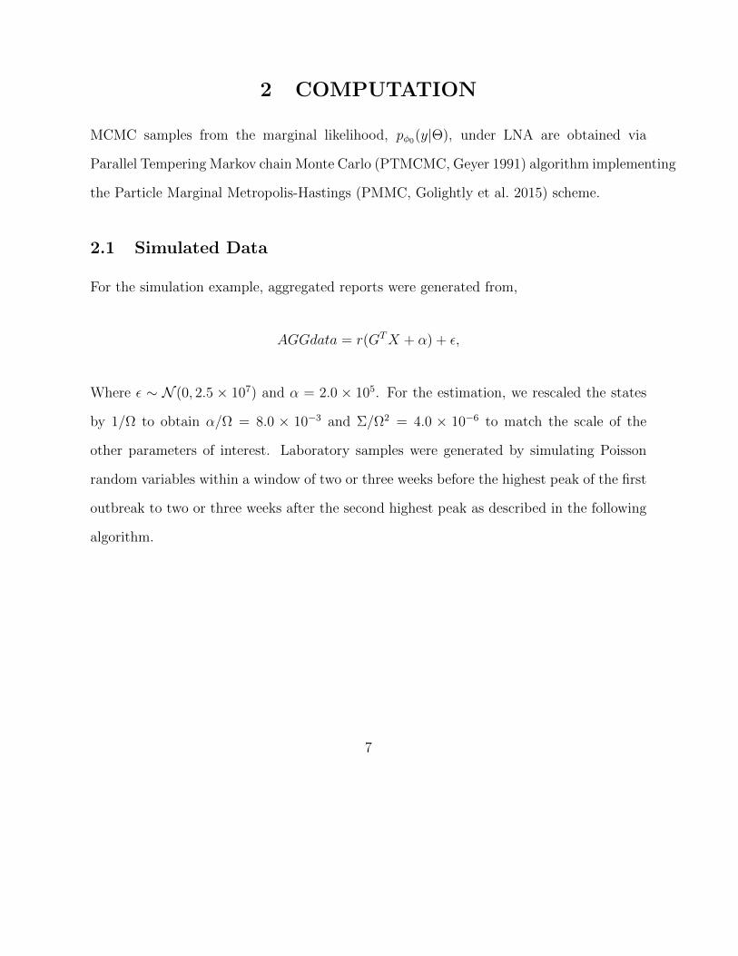
other parameters of interest. Laboratory samples were generated by simulating Poisson

random variables within a window of two or three weeks before the highest peak of the first

outbreak to two or three weeks after the second highest peak as described in the following

algorithm.

7

Algorithm 1: Laboratory Simulated Samples

Result: INFsample, RSVsample

begin

Take the interval of weeks between 2 weeks before and 2 or 3 weeks after the

highest peaks of the two modes (I)

Generate samples equal to the size of I, from a Poisson distribution.

for i in len(I) do

n = Ii, p =INFdatai

INFdatai +RSV datai

INFsample = Bin(n, p)

RSV sample = |n− INFsample|

3 NUMERICAL RESULTS

This section provides posterior summaries and pairwise correlation plots from the analysis

of each year considered in this study.

8

August 2002 - July 2003



β1 78.79 (65.55, 100.62) XSS 0.85 (0.63, 0.96)

β2 84.65 (72.83, 110.02) XIS 3.82× 10−6 (1.26× 10−10, 4.05× 10−5)

σ 1.05 (0.47, 1.38) XRS 0.02 (0.004, 0.04)

α/Ω 0.04 (0.02, 0.05) XSI 6.70× 10−5 (2.94× 10−9, 2.49× 10−4)

Σ/Ω2 4.85× 10−7 (4.22× 10−7, 1.34× 10−6) XRI 7.55× 10−5 (5.51× 10−9, 2.45× 10−4)

r 0.09 (0.07, 0.16) XSR 0.01 (0.003,0.03)

XIR 6.87× 10−6 (6.38× 10−10, 6.48× 10−5)

Figure 1: Pairwise marginal posterior plots for the model parameters (top panel) and initialconditions and auxiliary parameters (bottom panel) from the analysis in year 2002-03.

9




β1 87.86 (82.21, 111.28) XSS 0.92 (0.63, 1.00)

β2 73.05 (68.31, 94.23) XIS 5.51×10−6 (1.26×10−10, 4.05×10−5)

σ 1.19 (0.47, 1.38) XRS 1.37×10−2 (0.43, 3.57)×10−2

α/Ω 5.70×10−2 (3.50, 6.60)×10−2 XSI 1.44×10−5 (2.94×10−9, 2.49×10−4)

Σ/Ω2 5.58×10−7 (4.42, 0.10)×10−7 XRI 6.24×10−6 (5.51×10−9, 2.45×10−4)

r 5.95×10−2 (5.20, 8.60)×10−2 XSR 1.59×10−2 (0.28, 3.16)×10−2

XIR 7.61×10−6 (6.38×10−10, 6.48×10−5)


10




β1 71.78 (64.87, 94.58) XSS 0.91 (0.64, 0.94)

β2 69.84 (65.90, 95.31) XIS 3.49 ×10−7 (6.22 ×10−11,2.31 ×10−5)

σ 0.37 (0.12, 0.872) XRS 0.01 (0.003, 0.031)

α/Ω 0.02 (0.008, 0.02) XSI 9.42 ×10−5 (6.68 ×10−8, 2.58 ×10−4)

Σ/Ω2 4.76×10−7 ( 3.02,7.28)×10−7 XRI 6.80 ×10−5 (1.52 ×10−8, 2.46 ×10−4)

r 0.16 (0.13, 0.33) XSR 0.01 ×10−2 (0.004, 0.04)

XIR 4.19 ×10−6 (1.40 ×10−9,2.33 ×10−5)


11




β1 89.31 (70.45, 108.90) XSS 0.87 (0.63, 0.97)

β2 89.24 (71.53, 110.09) XIS 4.17×10−6 (3.43 ×10−10, 4.48 ×10−5)

σ 0.19 (0.05, 0.43) XRS 0.01 (0.003, 0.03)

α/Ω 0.04 (0.013, 0.041) XSI 1.73 ×10−6 (1.36 ×10−9, 9.34×10−5)

Σ/Ω 8.32×10−7 (4.83×10−7, 1.18 ×10−6) XRI 1.67 ×10−5 (4.72 ×10−9, 1.21×10−4)

r 0.09 (0.08, 0.21) XSR 0.0098 (0.0027, 0.03)

XIR 5.59e-06 (5.75×10−10, 8.14 ×10−5)


12




β1 74.26 ( 62.62, 99.95) XSS 0.85 ( 0.59, 0.95)

β2 74.67 ( 64.50, 101.57) XIS 1.617e-07 ( 2.31 ×10−10, 3.58 ×10−5)

σ 0.379 ( 0.09, 0.84) XRS 0.01 ( 0.005, 0.03)

α/Ω 0.016 ( 0.004, 0.02) XSI 6.23 ×10−5 (2.35×10−10, 2.36×10−4)

Σ/Ω2 7.075 ×10−7 ( 4.05, 9.9)×10−7 XRI 4.21 ×10−5 (3.21×10−9 , 1.69×10−4)

r 2.12 ×10−1 ( 0.14, 0.52) XSR 0.02 (0.003, 0.03)

XIR 8.43 ×10−6 (8.94×10−7, 3.23×10−5)


13




β1 79.12 (53.47,97.79) XSS 0.746 (0.47, 0.91)

β2 95.38 (77.11,125.70) XIS 3.47 −6 (3.69×10−11, 4.32 ×10−5)

σ 2.49 (1.46, 4.65) XRS 0.02 (0.007, 0.05)

α 0.09 (0.03, 0.10) XSI 2.79×10−5 (3.35×10−9, 1.78×10−4)

Σ 5.74×10−7 (3.68, 9.84) ×10−7 XRI 9.33×10−5 (3.13×10−9, 1.66×10−4)

r 0.04×10−2 (0.032,0.09) XSR 0.01 (0.003, 0.04)

XIR 5.97×10−7 (4.26×10−12, 4.07×10−5)


14

References

Geyer, C. (1991). Markov chain Monte Carlo maximum likelihood. In Computing Science

and Statistics, Proceedings of the 23rd Symposium on the Interface, 156. American

Statistical Association.

Gillespie, D. T. (2007). “Stochastic Simulation of Chemical Kinetics”. Annu. Rev. Phys.

Chem., 58:35–55.

Golightly, A., Henderson, D. A., and Sherlock, C. (2015). “Delayed Acceptance Particle

MCMC for Exact Inference in Stochastic Kinetic Models”. Statistics and Computing,

25(5):1039–1055.

Kamo, M. and Sasaki, A. (2002). “The Effect of Cross-Immunity and Seasonal Forcing in

a Multi-Strain Epidemic Model”. Physica D: Nonlinear Phenomena, 165(3):228–241.

Van Kampen, N. G. (1992). “Stochastic Processes in Physics and Chemistry”, volume 1.

Elsevier.

15

Documents

Identifying Individual Disease Dynamics in a Stochastic ... · Identifying Individual Disease Dynamics in a Stochastic Multi-pathogen Model From Aggregated Reports and Laboratory