Identifying Energy Waste through Dense Power Sensing andUtilization Monitoring

Maria Kazandjieva, Omprakash Gnawali, Brandon Heller, Philip Levis, and Christos KozyrakisComputer Science Lab, Stanford University

mariakaz,gnawali,brandonh,pal@cs.stanford.edu, christos@ee.stanford.edu

AbstractPowerNet is a hybrid sensor network for monitoring the

power and utilization of computing systems in a large aca-demic building. PowerNet comprises approximately 140single-plug wired and wireless hardware power meters and 23software sensors that monitor PCs, laptops, network switches,servers, LCD screens, and other office equipment. PowerNethas been operational for 14 months, and the wireless metersfor three months.

This dense, long-term monitoring allows us to extrapolatethe energy consumption breakdown of the whole building.Using our measurements together with device inventory wefind that approximately 56% of the total building energy bud-get goes toward computing systems, at a cost of ≈ $22,000per month. PowerNet’s measurements of CPU activity andnetwork traffic reveal that a large fraction of this power iswasted and shows where there are savings opportunities.

In addition to these sensor data results, we present our ex-periences designing, deploying, and maintaining PowerNet.We include a longterm characterization of CTP, the standardTinyOS collection protocol.

The paper concludes with a discussion of possible alterna-tives to computing system design that can save energy whilesatisfying user workloads.

1 IntroductionThis paper describes the design and deployment of Power-

Net, the first sensor network that monitors both power drawand utilization of computing devices in an office building.PowerNet provides fine-grained data on approximately 140devices, including many different desktops, monitors, net-work switches, and servers. Two types of power meters,wired and wireless, collect measurements once a second,while software sensors gather statistics on computer and net-work utilization. PowerNet has been active for 14 months,with the most recent deployment phase completed in January.

To date, “green computing” has focused primarily on thedata center, as it represents a large cost that lends well to cen-tralized control and optimization. This paper takes a differ-ent approach, examining a computing-heavy office building.Compared to a data center, this environment has a tremen-dously diverse set of devices that exhibit huge variations inworkload and configuration and exist under several overlap-

ping administrative domains. Improving the efficiency ofsuch a computing system requires detailed data of both en-ergy consumption and energy waste.

This paper makes four contributions. First, we extrapo-late a whole-building breakdown of energy consumption bycombining PowerNet data with surveys, observations, and ITdatabase records. We estimate that at least 56% of the build-ing’s $40,000 monthly electricity bill goes to its computingsystems infrastructure.1 Desktops and laptops consume 16%,30% goes to servers, 7% goes to monitors, and 3% of energygoes to networking.

Second, we quantify power variation between deviceclasses, within device classes, and for individual devices.This analysis identifies simple optimizations, such as changesin display settings, that lead to significant energy savings.

Third, PowerNet’s ability to correlate power consumptionwith utilization allows us to differentiate energy used wellfrom energy waste. This is an important difference from pre-vious work [8, 14]. We pinpoint examples of energy wastecaused by over provisioning, such as the wired building net-work. We also identify policies that prevent energy conser-vation, such as a nightly backup policy that requires desk-tops to be kept on overnight even though backups only takean hour. Finally, we turn the power and utilization data intoinsights for future computing infrastructure decisions: pur-chasing high-end vs thin-client desktops and the benefits ofintelligent power management.

Moreover, the nature, scale, and duration of the PowerNetdeployment yields insights for future indoor sensor deploy-ments. We present the first long-term study of CTP [7], thestandard TinyOS data collection protocol. We find daily andweekly cycles in CTP’s behavior, caused by human activity,and present a crippling bug whose fix has since been includedin the standard TinyOS release. Our experiences deployingPowerNet will inform future efforts to understand and reduceenergy consumption in office-style buildings.

2 OverviewThe PowerNet deployment collects power and utilization

data for the computing infrastructure of an office building.Figure 1 shows the overall design. The deployment currently

1Cooling and heating are through chilled water and steam, so arenot part of this total.

Device Type Count Utilization Count

Desktop 44 CPU 15Monitor 40Laptop 16 CPU 1Network Switch 11 traffic 7Printer 10Server 9Fridge 3Access Point 2External Hard Drive 2Fax Machine 1

Total: 138 23

Table 1. PowerNet covers a variety of devices whosepower measurements we use to characterize the energyconsumption of the whole building. We also monitor CPUutilization and network traffic.

includes 138 single-outlet, high-sampling-rate power meters,both wired and wireless. Each meter connects to exactly onecomputing device, such as a PC, display, or network switch;the full list is shown in Table 1. In addition, building oc-cupants and system administrators have volunteered to in-stall software to monitor CPU utilization and network traf-fic. All data is logged continuously to a central MySQLdatabase, from once a second to once a minute, dependingon the source. The system currently logs approximately 1GB per day from 161 data sources.

Wired Meters. The 55-node wired deployment is sparse,covering spread-apart wiring closets, student offices, and abasement server room. Commercially-available Watts Up.NET meters [10] transmit measurements over Ethernet, upto once a second, over the existing building network. Eachmeter posts data via HTTP to a server process on the Power-Net logging machine. These meters were a useful first step ingathering power data, though the practical issues of size andproprietary software (described later in Section 5.1) hinderedfurther deployment.

Wireless Meters. In contrast, the 85-node wireless de-ployment is dense, covering a large fraction of the power out-lets in one wing on one floor, shown in Figure 2. Custom-made low-power wireless meters transmit data from an ad-hoc multihop network. Each meter is a modified versionof the open-source ACme meter [14]. Each ACme includespower measurement circuitry and an Epic core with micro-processor and radio chip [11]. More hardware details can befound in Section 5.2.

The meter software, built on TinyOS, includes sampling,routing and dissemination capabilities. The top-level applica-tion reads power draw every second and sends a data packetafter buffering ten samples. The motes use CTP [7] as theunderlying routing layer. The code includes Deluge [13] forremote image upgrades. In addition to power data, the motesgather CTP statistics. Section 6 describes in detail the gath-ered data and the resulting observations. To our knowledge,this deployment is the largest, longest-term, and highest-density one using CTP, and one of the first to be done indoors.

Utilization Monitoring. PowerNet also monitors utiliza-tion, in addition to power, for 23 computing devices. On the

Figure 1. The deployment measures power usage and uti-lization of individual devices. The data is transmitted overthe network and stored on a central server.

Figure 2. The wireless power meter deployment spans onewing on one floor of an office building. The black squarerepresents the sink and every dot is a power meter. Mostmeters are located under desks, near the floor.

network side, an SNMP script polls seven network switchesonce a minute and records the average traffic in Mbps. Onthe PC side, we collect CPU utilization and the list of activeprocesses. Seven student PCs run a script that reads the /procvirtual file system to give average CPU load every second.Nine staff machines run a Windows script that reports the listof running processes (similar to the task manager) and totalCPU load. The combined data helps correlate power withobserved workload.

Data Storage The wired and wireless meters and CPUmonitors send the data to a central server with two 1.8 Ghzcores and 2 GB of RAM. With over 160 sensors reportingas often as once a second, data piles up quickly. Section 5.3describes the backend scalability challenges.

Data Access and Analysis The data stream providesnear-real-time feedback to building residents, equipment pur-chasers, and system administrators through the PowerNetwebsite. A display in the building lobby provides informa-tion about the project, along with graphs showing real-timepower consumption of categories of devices, such as moni-tors, servers, and network equipment.

Sun Mon Tue Wed Thu Fri Sat0

100

200

300

400

500

Aggr

egat

e Po

wer

(kW

)

Desktops and Laptops (16%)

Servers (30%)

LCD Displays (7%)Switches (3%)

Rest of Building (44%)

Sun Mon Tue Wed Thu Fri Sat0

100

200

300

400

500

Aggr

egat

e Po

wer

(kW

)

Desktops and Laptops (16%)

Servers (30%)

LCD Displays (7%)Switches (3%)

Rest of Building (44%)

Figure 4. Aggregate power draw for the entire PowerNet building shows diurnal and weekday/weekend patterns. Com-puting systems account for 56% of the total 445 kW. The given week of data is representative of the building, exceptMonday which was a university holiday (Feb 15).

12am 4am 8am 12pm 4pm 8pm 12am

2

4

6

8

10

Aggr

egat

e Po

wer

(kW

)

43 Desktops

9 Servers

11 Switches

40 LCD DisplaysOther

12am 4am 8am 12pm 4pm 8pm 12am

2

4

6

8

10

Aggr

egat

e Po

wer

(kW

)

43 Desktops

9 Servers

11 Switches

40 LCD DisplaysOther

Figure 3. PowerNet’s measurements account for 2.5% ofthe building’s power consumption.

However, power feedback for building residents is not thefocus of this paper. Our goal is to answer building-level ques-tions about where energy is going and how we change man-agement processes and purchasing decisions to reduce en-ergy consumption. At the heart of this paper are the insightsrevealed by over 150 gigabytes of collected and correlatedpower and utilization data. What follows are our findings –expected in some cases, and surprising in others.

3 Computing Energy ConsumptionThis section analyzes the power data that PowerNet has

collected. It examines three classes of devices in detail: dis-plays, computers, and networking switches. Before Power-Net, the building manager’s only view into energy consump-tion was a monthly electricity bill of approximately $40,000.Using PowerNet’s measurements, network activity logs, asurvey of building occupants, and cross-correlating with ITdatabases, we find that computing systems draw on average252kW: 56% of the building’s 445kW. We find that displays

are responsible for 50% of the building’s diurnal power drawvariations. There are significant activity and power profilevariations within a device class, such that dense sampling isnecessary for accuracy: for example, sampling only 5 randomdesktops has a 5th percentile error of underestimating by 31%and a 95th percentile error of overestimating by 40%.

3.1 The Big PictureFigure 3 shows the power draw of PowerNet’s 140 devices

over a 24-hour period. The 9 to 11kW draw is 2.5% of thebuilding total. Each layer represents a different device cate-gory. The largest contributors are labeled. Consumption ofmost devices is fairly steady, with the exception of displays.Although the measured displays are responsible for a 14%increase in the measured power draw, effective power man-agement reduces their total energy contribution to only 7%.Weekends see power profiles similar to Figure 3, althoughvariations are smaller because fewer displays are turned on.Overall, displays are almost completely responsible for thevariation we see in computing power.

Even though PowerNet only measures 2.5% of the build-ing power, by combining these samples with other informa-tion about the distribution of computing devices, we can ex-trapolate to the whole building, as in Figure 4. Specifically,from network administrator databases of active nodes, emailsurveys, and manual inspections of networking closets andserver rooms, we can generate a reasonable inventory of de-vices in the building. We can use PowerNet’s measurementsto couple this inventory to power draw.

Using PowerNet as a motivation, we convinced campusservices to provide Excel spreadsheets of the building’s aver-age draw over 15-minute intervals. The top curve in Figure 4shows one week of this data. Finer-resolution data makesit easy to spot expected trends such as day/night and week-day/weekend patterns: daytime sees a 30% increase in power

Device Type Measured Total Extrapolated via Total Draw Uptime % of Building

Desktops/Laptops 44 742 whois, MAC address registrations 70 kW 24 hrs/day 15%Servers 9 500 manual inspection 137 kW 24 hrs/day 30%LCD Displays 40 750 occupant survey 61 kW 12 hrs/day 7%Switches 11 62 network admin records 15 kW 24 hrs/day 3%

Table 2. We cross-correlate PowerNet measurements with IT databases to extrapolate energy consumption of computingsystems in the whole building.

Type # Count Power Draw(watts)

HP 5406zl (6-slot) 20 325HP 5412zl (12-slot) 8 500HP 2724 2 100Cisco Cat 6509 2 400Cisco Cat 4000 2 600Cisco Cat 3750G 2 160Linksys 2 50NEC (misc) 5 100Cisco (misc) 5 100Quanta (4-slot) 5 50Others 9 50

Total: 62

Table 3. Summary of groups of switches with individ-ual and estimated total power consumption. This inven-tory includes all major network switches in the PowerNetbuilding.

draw over nighttime. Figure 4 also shows our estimate ofcomputing’s contribution to this power draw for the sameperiod. Computing systems are responsible for 56% of thebuilding’s total energy consumption. Furthermore, displaysare responsible for a 46kW increase in daytime power drawor 50% of the total increase.

The rest of this section examines displays, desktops, andswitches in greater detail and explains how we perform thisextrapolation. Table 2 shows our extrapolation methodologyand results at a glance.

3.2 Networking EquipmentWe compute the energy consumption of the building’s net-

working infrastructure (its Ethernet switches and WiFi accesspoints). In the PowerNet building, network access is pro-vided by 2 core switches located in the basement and 26 edgeswitches spread across the five floors. In addition, there are anumber of smaller switches, deployed in ad-hoc ways by in-dividuals or research groups. Table 3 presents an inventory ofnetworking equipment. While we can account for all majorswitches, finding all of the small ones (e.g., 4-hub Linksysswitches) was not possible due the scale of the building andpermissions required. Since the infrastructure is planned by asmall number of administrators and centrally purchased, theequipment used is comparatively uniform: over half of theswitches are a single model, the HP5406zl.

Figure 5 show the power consumption of three switches.Power draw variation is negligible and the small peaks arelikely due to CPU spikes. Networking infrastructure powereasy to characterize; future deployments need not collect fine-

12am 4am 8am 12pm 4pm 8pm 12am

Time

0

100

200

300

400

500

Pow

er (w

atts

)

HP 5412zl, 12-slot, 96 active ports

HP 5406zl, 6-slot, 72 active ports

NEC, 48 active ports

Figure 5. Switch power consumption is constant, barringtransient ups or downs likely due to fans. Thus, the net-working infrastructure does not require long-term powermonitoring.

grained long-term samples, since the data rarely changes. Weuse measurements from the core and edge switches and cross-correlated that to data-sheet-reported values to estimate thetotal energy consumption. On average, the switches in thebuilding consume 15 kilowatts. This comes to a total of12000 kWh per month, 3% of the building’s total consump-tion.

3.3 Computer DisplaysWith the recent shift from CRTs to large LCDs, displays

have become a significant contributor to electricity bills. Thissection examines PowerNet’s display power measurementsand explains how we extrapolate to the energy consumed byall displays in the building.

Over 600 people use the PowerNet building as officespace. PowerNet’s power meters and utilization sensors covera broad and diverse range of residents, including students,professors, visitors, servers, and administrators. While thisdiversity allows us to see a breadth of usage patterns, it consti-tutes a highly biased sample. In practice, most of PowerNet’soffices are occupied by graduate students. Therefore, simplyusing a multiplicative factor on PowerNet’s measurementscould be highly inaccurate. For example, administrators tendto have lightweight desktops and smaller LCDs, while manystudents have powerful desktops and larger LCD displays.

PowerNet’s measurements allow us to quantify the aver-age power draw of a class of display; extrapolating to whole-building power draw requires knowing the distribution of dis-play classes. To obtain a reasonably accurate estimate of

Size Count Avg. Power

< 17” 917” to 19” 33 35 W20” to 22” 40 50 W23” to 25” 84 66 W26” to 27” 15 120 W29” to 30” 42 135 W> 30 2

Table 4. A survey shows that majority of building occu-pants use mid-sized LCD displays. Equipment upgradescause the number of large (30”) monitors to increase.

this distribution, we distributed an online survey asking oc-cupants for the number, size, and manufacturer of the com-puter screens they use. Table 4 presents data from the 169responses reporting 225 monitors and indicating the distri-bution of sizes. The majority of people use 23- to 25-inchmonitors. 30” screens are the second largest population.

Table 4 also shows the power consumption the specifica-tion sheets of different displays report. PowerNet’s measure-ments reveal that there is a great variation in active powerdraw even between devices of the same size and make. Weconducted a controlled test to see how different display set-tings affect monitor power draw. We chose a 30” Dell moni-tor, partially to highlight the differences in monitor states, butalso because these displays form an increasing portion of thedisplay population.

Figure 6 shows an hour-long data trace during which weadjusted the monitor brightness and desktop color scheme.Depending on the monitor brightness settings and the colorsin the image displayed, the power draw varies by up to 35W(25%). Lowering the brightness by two settings (pressingthe ’-’ button twice) reduced the average power draw from145 to 117 watts, a 19% reduction in consumption. Addi-tionally, LCD power draw is affected by the colors displayed.More energy aligns more liquid crystals in each pixel, permit-ting more light to shine through and enabling them to displaybrighter colors. Thus, a 30-inch monitor has maximum powerdraw, measured at 145 watts, when the majority of the screendisplays white elements. Switching to a dark background andcolor scheme or viewing darker web pages reduces the drawto 127 watts. Displaying dark colors with the lower bright-ness setting reduces power draw to 110W.

With a good understanding of individual power, we cancharacterize the effect at scale. In order to account for allmonitors in the building, we extrapolated from the surveydata and typical power draw. From building inventory andnetwork reports of what computers are active, we were ableto estimate that the PowerNet building has approximately 750displays. We assume that these 750 displays follow the samesize distribution as gathered in the survey and that they followthe same use distribution as the metered monitors, as there isno significant difference in monitor activity between classesof residents. These calculations indicate that on average, amonitor draws just over 80W, with 750 monitors drawing 61kW. Since most displays are powered on about 12 hours a day,this translates to 7% of the building total energy.

0 2 4 6 8 10 12 14Time (minutes)

40

80

120

160

Pow

er (w

atts

)

max brightness

~145 W

sleep~7 W

(max-2) brightness

~117 W ~110 Wdark colors

Figure 6. The power consumption of a computer moni-tor varies widely depending on its settings. Minor adjust-ments of brightness level can result in 20% savings forlarge monitors.

3.4 Personal ComputersPersonal computers – dekstops and laptops – and servers

are the largest contributor to the computing infrastructure en-ergy consumption. According to the department’s database ofregistered devices there are ≈1250 machines active on thebuilding’s network. This number includes student, staff, andprofessor machines as well as server machines located in twoserver rooms. We manually inventoried the server rooms todistinguish what portion of the 1250 are desktops or laptopsand what portion are servers. Of this total, 500 machines areservers, while the rest are laptops or desktops. We refer todesktops and laptops as personal computers (PCs), as manylaptops are used with docks.

PowerNet measurements of 44 PCs show that desktopsvary greately in power draw – anywhere from 40 to 350 watts.Figure 7 shows the power consumption of three different PCsover 24 hours. Desktop ‘a’ is a Dell Inspiron 530 desktopwith a powerful graphics card; desktop ‘b’ custom-built ma-chine and desktop ’c’ is a lightweight Dell Optiplex 745.Power consumption varies widely, not only between desk-tops, but also for the same desktop in time.

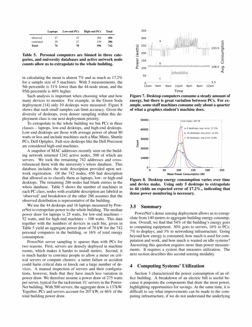
Figure 7 shows that dense, fine-grained, long-term instru-mentation is the key to accurately characterizing the powerconsumption of a building’s computers. To explore this fur-ther, we run statistical analyses on the average desktop con-sumption. The average power draw of the 44 measured desk-tops is 107 watts. What error could we expect if only 5, 10,or 20 of the desktops were monitored? To estimate the er-ror with only 5 desktops, we generated 1,000,000 random 5-tuples drawing from the lists of 44 desktops. Next, we cal-culated the mean for each set of 5 machines and plotted ahistogram of the results. The experiment was repeated for10- and 20-tuples of computers.

Figure 8 shows the three resulting histograms with the 44-node mean indicated by a vertical line. As expected, largersample sizes yield a narrower spread, with averages that arecloser to the mean. We calculate the expected error by av-eraging over the probabilities of all possible mean values asgiven by the histogram. With 20 desktops , the expected error

Laptops Low-end PCs High-end PCs Total

observed 47 43 366 456estimated 29 27 230 286Total 76 70 596 742

Table 5. Personal computers are binned in three cate-gories, and university databases and active network nodecounts allow us to extrapolate to the whole building.

in calculating the mean is almost 7% and as much as 17.2%for a sample size of 5 machines. With 5 measurements, the5th percentile is 31% lower than the 44-node mean, and the95th percentile is 40% higher.

Such analysis is important when choosing what and howmany devices to monitor. For example, in the Green Sodadeployment [14] only 10 desktops were measured: Figure 8shows that such small samples can limit accuracy. Given thediversity of desktops, even denser sampling within this de-ployment class is our next deployment priority.

To extrapolate to the whole building we bin PCs in threeclasses – laptops, low-end desktops, and high-end desktops.Low-end desktops are those with average power of about 80watts or less and include machines such a Mac Minis, ShuttlePCs, Dell Optiplex. Full-size desktops like the Dell Precisionare considered high-end machines.

A snapshot of MAC addresses recently seen on the build-ing network returned 1242 active nodes, 500 of which areservers. We took the remaining 742 addresses and cross-referenced them with the university’s whois database. Thisdatabase includes the node description provided upon net-work registration. Of the 742 nodes, 456 had descriptionthat allowed us to classify them as laptops, low- or high-enddesktops. The remaining 286 nodes had blank entries in thewhois database. Table 5 shows the number of machines ineach PC class; nodes with available description are labeled as‘observed’ and breakdown of the other 286 assumes that theobserved distribution is representative of the building.

We use the 44 desktops and 16 laptops measured by Pow-erNet to extrapolate power to the whole building. The medianpower draw for laptops is 25 watts, for low-end machines –52 watts, and for high-end machines – 108 watts. This datatogether with the numbers of devices in each bin, given inTable 5 yield an aggregate power draw of 70 kW for the 742personal computers in the building, or 16% of total energyconsumption.

PowerNet server sampling is sparser than with PCs fortwo reasons. First, servers are densely deployed in machinerooms, which makes it harder to install meters. Second, itis much harder to convince people to allow a meter on crit-ical servers or compute clusters: a meter failure or accidentcould harm critical data or knock out a large number of de-vices. A manual inspection of servers and their configura-tions, however, finds that they have much less variation inpower draw. We therefore assume a power draw of 275 wattsper server, typical for the rackmount 1U servers in the Power-Net building. With 500 servers, the aggregate draw is 137kW.Together, PCs and servers account for 207 kW, or 46% of thetotal building power draw.

12am 4am 8am 12pm 4pm 8pm 12am

Time

0

50

100

150

200

250

300

350

Pow

er (w

atts

)

5.5

108.5

233.5

Avg.

Con

sum

ptio

na

b

c

Figure 7. Desktop computers consume a steady amount ofenergy, but there is great variation between PCs. For ex-ample, some staff machines consume only about a quarterof what a graphics student’s machine does.

0 50 100 150 200 250Mean Power Consumption (W)

0

10000

20000

30000

40000

50000

Coun

t

a

b

c a: 5 desktops, exp. error: 17.2%

b: 10 desktops, exp error: 11.5%

c: 20 desktops, exp error: 6.8%

true mean: 107 W

0 50 100 150 200 250Mean Power Consumption (W)

0

10000

20000

30000

40000

50000

Coun

t

a

b

c a: 5 desktops, exp. error: 17.2%

b: 10 desktops, exp error: 11.5%

c: 20 desktops, exp error: 6.8%

true mean: 107 W

Figure 8. Desktop energy consumption varies over timeand device make. Using only 5 desktops to extrapolateto 44 yields an expected error of 17.2%., indicating thatdense power monitoring is necessary.

3.5 SummaryPowerNet’s dense sensing deployment allows us to extrap-

olate from 140 meters to aggregate building energy consump-tion. Overall, we find that 54% of the building’s energy goesto computing equipment. 30% goes to servers, 16% to PCs,7% to displays, and 3% to networking infrastructure. Goingbeyond how energy is consumed, how much is used for com-putation and work, and how much is wasted on idle systems?Answering this question requires more than power measure-ments. It requires a system that measures utilization. Thenext section describes this second sensing modality.

4 Computing Systems’ UtilizationSection 3 characterized the power consumption of an of-

fice building. A breakdown of an electric bill is useful be-cause it pinpoints the components that draw the most power,highlighting opportunities for savings. At the same time, it isdifficult to say what improvements can be made to the com-puting infrastructure, if we do not understand the underlying

Sun Mon Tue Wed Thu Fri SatTime

0

20

40

60

80

100CP

U (%

)

0

100

200

300

Pow

er (w

atts

)

CPU

Power

Figure 9. A week-long trace of power consumption and CPU utilization shows idle periods during which the power-hungry desktop could have been turned off.

usage patterns that require computing in the first place. Thissection digs deeper into the meaning of energy efficiency bycorrelating power consumption with device utilization.

In an ideal world, all systems would be power propor-tional, drawing power when work is done, and consumingnothing when the system is idle or unused. Reality is not sokind. We examine the utilization of computers and networkswitches. The key insight is that current systems, computingor networking, are heavily underutilized. This fact, combinedwith large baseline power consumption, means that energyefficiency is extremely low. A large portion of the time, elec-tricity bills pay for unused or under-utilized devices.

4.1 CPU UtilizationThe aggregate power graphs at the beginning of Section 3

suggest that most computers are rarely turned off. Figure 9shows power consumption and CPU utilization for one spe-cific computer over 1 week. Usage patterns are immediatelyobvious: there are long idle periods at night and on weekends.While machine utilization varies greatly over the span of aweek, from 0% to 60%, this desktop’s draw never drops be-low 220 watts. Measurements from multiple desktops showan additional cost of roughly one watt for every 1% increasein CPU utilization beyond idle.

If these computers are mostly idle, then why are they notbeing put to sleep? Going back to Figure 7, only one of thethree machines was put to sleep during non-business hours,while the other two remained on. We do not see strong diur-nal variation in building power consumption largely becauseresidents are not taking advantage of the sleep and hibernatestates provided by modern OSes, especially during nighttimehours.

The reasons for this behavior vary but most often peoplecite unwillingness to wait for machine startup in the morning,ability to access the machine remotely, and nightly backups.On several accounts, staff members in our department sharedthat they would love to put their computers to sleep at the endof the workday but are not allowed to do so. Backups arescheduled to begin at 8:45 pm. Backups are one example ofa workload that requires a machine to be powered on.

The energy waste from always-on computers is only halfthe story. Further examination of CPU data shows that evenwhen actively used, most computers are rarely pushed to theirprocessing limits. Table 6 shows the the 5th, 50th, and 95th

percentiles of CPU utilization for seven student machines.The data was collected every 1 second for the past 11 months.

Percentile CPUMachine Type 5th 50th 95th

high-end custom-built 0% 1% 57%Dell Optiplex 745 1% 9% 58%Dell Precision T3400 0% 4% 29%Dell Precision T3400 0% 1% 13%Dell Inspiron 530 1% 1% 8%HP Pavilion Elite m9250f 0% 0% 25%Dell Precision T3400 0% 1% 7%

Table 6. CPU utilization for 7 student machines collectedover 11 months reveals high under-utilization.

The measured computers rarely use even 50% of their avail-able CPU.

This observation raises the question of whether powerfuldesktops are the best way to provide computing power tousers. The trends we see are towards upgrading to more pow-erful machines, yet typical workloads hardly tax the avail-able CPU resources. Section 7 goes further into alternativeproviding computing systems that meet user needs in a moreenergy-efficient manner.

4.2 Network TrafficIn Section 3 we found that the networking infrastructure

consumes much less energy than desktops. We also noted thatswitches consume a constant amount of power. This promptsthe questions of how much traffic is flowing through the 60 orso switches in the building, and whether that traffic changeswith time.

Figure 10 shows the traffic coming into one of the fourswitches on the second floor of our building. This is an HPProcurve switch with 96 1-gigabit active ports, consuming500 watts. Over one week in March, bandwidth demandnever exceeded 200 Mbps – an amount that could be handledby one gigabit port instead of 96

To verify that this is not aberrant behavior, Figure 11shows the cumulative distribution of traffic for 7 buildingswitches. Note that the x-axis has a log scale. Table 7 ac-companies the figure with a list of switch types we measureand the length of each data trace.

Similar to computers, switches are highly underutilized.For the equipment we measure, total network demand islower than 1000 Mbps 100% of the time. Of course, net-work over provisioning is not a new concept or observation;it provides benefits, including higher throughput, lower loss,

Sun Mon Tue Wed Thu Fri SatTime

050

100150200

Traf

fic (M

bps)

Figure 10. Typical traffic patterns for one edge switches in the building. Network utilization remain low. Power con-sumption for this switch remain constant, at approximately 500 watts.

10-2 10-1 100 101 102 103

Traffic (Mbps)

0.00

0.25

0.50

0.75

1.00

CDF

ab

c de

f

g

10-2 10-1 100 101 102 103

Traffic (Mbps)

0.00

0.25

0.50

0.75

1.00

CDF

ab

c de

f

g

Figure 11. CDF of traffic for seven switches over 6 monthsshows that switches are operating well under capacity.

Label Switch Type Active Ports Datatrace(gigabit each) (# days)

a HP 5412zl 120 150b HP 5406zl 96 40c HP 5412zl 120 40d HP 5406zl 72 150e NEC IP8800 24 420f HP 5412zl 24 420g NEC IP8800 48 420

Table 7. Summary of groups of switches with individualand estimated total power consumption. Gates building.

and lower jitter. When the average utilization is under onehundredth of one percent, several questions beg an answer.Is the amount of over-provisioning unnecessarily large? Howcan we take better advantage of the large amount of band-width that today’s networks are ready to support? We discusspossible answers to these questions in Section 7.

5 Deployment ExperiencesPrior sections presented the data that PowerNet has col-

lected. The next two sections present our experiences deploy-ing PowerNet. This section describes in detail our monitoringinfrastructure for collecting power and utilization data. Pow-erNet uses two types of power meters to collect data; the firstare commercial off-the-shelf, while the second are custom-made. We also share experiences and lessons learned overthe lifetime of the deployment.

5.1 Wired DeploymentThe initial requirement for the power meters was the abil-

ity to sense individual outlets at high sampling rates. This dif-fers from many residential solutions that track whole-houseenergy consumption and report data every 10 or more min-utes. Commercially-available Watts Up .NET meters werethe first power sensors in the deployment, since they wereeasy to obtain [10]. These meters transmit measurements overEthernet, up to once a second. Meters were placed in wiringclosets, the basement server room, and spread-apart offices.While these meters were a useful first step in gathering powerdata, deploying and maintaining them proved to be difficult;problems surfaced even before the deployment began.

The first practical issue was the lack of in-field upgradablefirmware. When a bug was discovered in the TCP stack, ouronly option was to pack up four large boxes of power metersand send them back, so that company staff could fix the pro-prietary code. After several weeks, the meters were back inour possession and the deployment could begin.

It quickly became clear that few offices had an open Eth-ernet port for each power meter. Many offices required addi-tional small Ethernet switches and extra cables. The volunteerparticipants were unhappy with the clutter under their desks,due to the size of the meters. Each one weighs 2.5 lbs, with athick, six-foot-long cord leading to a 7” x 4” x 2” base. De-spite the physically clunky deployment experience, we wereable to install 80 meters.

In the PowerNet building, each device must have a MACaddress registration to obtain an IP address. Each groupwithin the building has a unique VLAN, and each meter wasstatically registered to a group. The registrations could not bedone all at once, since neighboring offices may correspondto different groups, and we could not know in advance howmany meters would be needed for a given office. The networkadmins were burdened by the power meter registrations, andwith this much manual configuration, mistakes happened.

We received an email from a network admin stating that“more than half of all DNS lookups emanating from [the threeEngineering buildings] to the campus servers” were comingfrom the power meters. The solution for the lack of DNScaching was to go back to each meter, plug it into a laptop viaUSB, and hard-code the IP address of the PowerNet server.

In addition to DNS lookups, the meters were also mak-ing ARP requests once per second and overwhelming the net-work security monitoring infrastructure. We received anotheremail from the IT staff, pointing out that ”[t]he 70 currentmeters now account for 20% of total daily recorded flows”

by the security system. To work around this problem, thelogging server was moved to a special VLAN that was notmonitored by the network admins. That resulted in an IP ad-dress change, which meant yet another trip to the individualmeters to update the hard coded IP address of the server.

Once the deployment was in place, we observed a num-ber of meter software errors. From the 90 power meters, 8completely stopped working; they did not power up or didnot send or display any data. Another set of 5 to 7 meters be-gan reporting incorrect data at some point of the deployment;from the reported numbers we guess it was an integer over-flow issue but the closed firmware did not allow us to verifythis. The erroneous data was purged from the analyzed datasets. There were also some meters that would stop reportingdata over the network until they were rebooted. That againwas likely a software problem where the meters were revert-ing to logging data locally instead of pushing it out via HTTP.Of the original 90, only 55 are still in operation; a number ofresidents simply unplugged their meters.

To their credit, the wired meters generally reported ac-curate data and work well for a dispersed deployment suchas the wiring closets. However, three key issues made thewired meters unsuitable for large-scale deployment: the lackof code accessibility and remote firmware upgrade, the over-head of installing the meters within the building network, anduser dissatisfaction with clutter and frequent maintenance.These experiences suggest that zero-configuration networksthat automatically form distinct subnets (e.g., as is proposedin RPL [6]) would improve ease of deployment.

5.2 Wireless DeploymentOpen-source low-power wireless meters were the main

candidates for expanding the PowerNet deployment - in par-ticular, the wireless ACme meters used in the Green Sodaproject [14]. The PowerNet wireless meters are based on theACme design, with two small modifications. The first wasa switch from a solid-state relay to a mechanical one. Thischange enabled a sealed case, by removing the need to ma-chine side slits to dissipate heat from the solid-state relay.The second change was to add an expansion port with a rangeof serial interfaces, to support new sensors and added storage.The cost per meter was about $120, as compared to $189 forthe wired meters, both in quantities of 100.

The deployment of 85 wireless meters took several after-noons, compared to two weeks for the wired meters. The ben-efits of the wireless deployment were noticed immediately,and some users even requested that we replace their wiredmeters with wireless ones. The IT staff was not burdened bymeter registrations, and the open nature of the software andhardware made modifications easy. The main meter limita-tion is transmission distance. Since the PowerNet wirelessdeployment focuses on a single wing of a building, the rangewas sufficient for CTP to form a mesh without a need for re-peaters.

5.3 Backend and Scalability ChallengesThe PowerNet infrastructure currently gathers 1GB of data

every day and this number will grow with the next round

Figure 13. Logical topology of the wireless network. Theroot of the tree is on top, and the number of nodes at eachlevel is shown.

of utilization sensors and 300 more wireless power meters.When the logging server was originally purchased we did notexpect to have scalability issues. One of the challenges weran into was that the server had two main roles – collectingdata and providing data. The later refers to the fact that weshare all data with users via a website and a display in thebuilding lobby.

A few months into the deployment, the amount of gath-ered data became large enough that displaying a week-longtimeline for a single device would take prohibitively long;generating a summary graph for all devices on the fly wasout of the question. Thus, PowerNet periodically runs a set ofdata summary calculations. For example, every 5 minutes theserver establishes what meters are reporting, takes the fine-grained data, averages it, adds it up, and produces a graphlike Figure 3.

A couple of times we observed that the server load was sohigh due to nightly scheduled backups and both MySQL andrsync experiences issues. The scalability and performance is-sues we have observed so far have prompted us to considera number of back-end improvements. These include partialdatabase backups via the binary log option in MySQL andincremental pre-calculations to summarize data. In the fu-ture, we plan to extend the system by one or more additionalservers and distribute the load and backup responsibilities.

6 Wireless Meter NetworkThe prior section examined our experiences with the over-

all PowerNet deployment. This section dives into the per-formance of the wireless network, specifically the CollectionTree Protocol. We chose CTP because it is the standard pro-tocol in TinyOS 2.x and extensive testbed experiments overthe scope of hours indicate that it is robust and efficient [7].This section examines whether CTP exhibits similar perfor-mance and behavior in an operational sensor network overa three month period, a timescale two orders of magnitudelarger than the prior study. Figure 2 shows the physical mapof the wireless deployment, while Figure 13 presents a snap-shot of the logical topology as constructed by CTP.

Because the wireless network does not have a wired backchannel, we add instrumentation to CTP to report statisticssuch as data transmissions, retransmissions, and receptions,beacon transmissions, and parent changes every 5 minutes.PowerNet uses 802.15.4 channel 19, which overlaps withheavily used WiFi channel 6. We chose this so we wouldnot interfere with research using quieter channels (e.g., 25and 26) and so that we could measure CTP in a less forgivingenvironment.

0 15 30 45 60 75 90

Num

ber

of N

odes

Time (days)

DeploymentPhase

A B C D E F G H I J K

5 10 15 20 25 30 35 40 45 50 55 60 65 70 75 80 85 90Jan 1 Feb 1 Mar 1

Figure 12. Number of nodes from which packets were received at the basestation during the deployment.

Label Date Duration Description

A Jan 19 9 hrs Building power outageMySQL recovery

B Jan 21 10 hrs Backend maintenance/backupC Jan 30 1 hr Basestation maintenanceD Feb 4 9 hrs Basestation software failureE Feb 8 1 hr Backend maintenanceF Feb 28 0.5 hr Backend maintenanceG Mar 8 34 hrs Backend disk failureH Mar 9 83 hrs Backend disk replacementI Mar 14 9 hrs Basestation bufferingJ Mar 18 7 hrs Basestation bufferingK Mar 22 4 hrs Backend RAID1 rebuild

Table 8. System Outages

6.1 Summary of Results

Overall, the backend collected 85.9% of the expected data.Of the 14.1% of missing data, 8.2% is due to backend failures,such as whole-building power outages or server disk failures.This type of failures also affected data from the wireless me-ters and utilization sensors. Of the remaining 5.9%, we ap-proximate that 2.8% is due to users taking meters offline byunplugging them: the remaining 3.1% of data losses are dueto CTP.2

Sifting through CTP’s periodic reports, we find weeklyand daily cycles of topology adaptation that correspond to hu-man activity in the building. These periods of adaptation see asignificant increase in control traffic as well as increased pathcosts. In the middle of the night, the average cost (transmis-sions/delivery) of the network is just under 2, while duringthe day it can climb as high as 6. We find that CTP’s datap-ath validation leads to a tiny fraction (1 in 20,000) of packetstaking 10-100 times as many hops as normal, as they bouncethrough the topology repairing loops. Finally, we present abug we discovered in CTP’s link estimator where nodes areunwilling to route through a rebooted node for a very longtime, which can be disastrous if a base station reboots. Wepresent a fix to the bug, which the CTP maintainers have in-corporated into the recent TinyOS 2.1.1 release.

2We assume the CTP delivery for the days 39-59 to be represen-tative for the full deployment period.

Nodes 85Path Length 1.84Cost 1.91Cost/PL 1.04Churn/node-hr 5.04Avg. Delivery 0.9695th % Delivery 0.789Loss Retransmit

Table 9. High-level CTP results, following the metrics inthe CTP paper [7]

6.2 System UptimeFigure 12 shows a 90-day trace of the number of connected

wireless meters reported for each 15-minute period. Over the90 days, the network experienced 11 network-wide outagesin data logging, labeled (A–K). Table 8 describes each out-age, including whole-building power loss, backend downtimemaintenance, disk failures, and gateway PC software failure.Overall, the backend was down for days, giving PowerNet anuptime of 91%.

Small dips in the number of reporting nodes (e.g., thetwo dips at 15 days) represent logging delay due to MySQLbuffering. These delays do not denote data loss.

While the high point of the plot remains stable (e.g., be-tween points D and F), it does vary. For example, a weekaround K (days 77-84) shows 8 nodes stopped reporting. Thisis not a network failure: the eight nodes were all in the sameroom (the labeled room in Figure 2). The 8-node outage oc-curred when the room was repainted and all computing equip-ment was unplugged and moved. Other, smaller dips repre-sent users unplugging meters. Generally speaking, no datadelivery outage observed was due to a failure in CTP or thewireless meter network. This deployment data validates priortestbed results on CTP’s robustness [7].

6.3 CTP PerformanceTo isolate CTP’s performance from network and node

downtime, all of these following results are from a 20-dayperiod in February (days 39-59 in Figure 12.) CTP’s behav-ior in this particular 20-day period is representative of the restof PowerNet’s lifetime after deployment.

Table 9 shows high-level results following the methodol-ogy used in the CTP publication [7]. The PowerNet networkbehaves differently than any of the studied testbeds. On one

M T W Th F SaSu M T W Th F SaSu M T W Th F Sa1

2

3

4

5

6

7

8C

ost

(tr

ansm

issi

ons/

deliv

ery

)

Data (95.7%)

Control (4.3%)

M T W Th F SaSu M T W Th F SaSu M T W Th F Sa1

2

3

4

5

6

7

8C

ost

(tr

ansm

issi

ons/

deliv

ery

)

Data (95.7%)

Control (4.3%)

Figure 14. Average packet delivery cost over 20 days.Weeknights and weekends show lower cost due to theavailability of more efficient and stable paths. Cost of 1is optimal.

Mid 4AM 8AM Noon 4PM 8PM Mid

2/9/2010

1

2

3

4

5

6

7

8

Cost

(tr

ansm

issi

ons/

deliv

ery

)

Data (89.2%)

Control (10.8%)

Mid 4AM 8AM Noon 4PM 8PM Mid

2/9/2010

1

2

3

4

5

6

7

8

Cost

(tr

ansm

issi

ons/

deliv

ery

)

Data (89.2%)

Control (10.8%)

Figure 15. CTP’s packet delivery cost over one day; avalue of 1 is optimal.

hand, its cost per path length of 1.04 indicates that intermedi-ate link are rarely used. (on average out of 104 packets only4 were retransmission), making it similar to testbeds such asMirage. On the other hand, its high average churn rate of 5.04per hour makes it similar to harsher testbeds such as Mote-lab. This indicates that while PowerNet has many high qual-ity links, those links come and go with reasonable frequency.

CTP’s average delivery ratio was 96.9% and only five outof the 85 nodes reported delivery ratio below 90%. Two ofthese nodes were near many other wireless nodes, while an-other two were in the corner, possibly using longer links. Theprincipal cause of packet loss is retransmission failure: CTPdrops a packet after 30 attempts to transmit it on a single link.

Figure 14 shows CTP’s average cost (transmissions/deliv-ery) over a 20 day period divided into data transmissions andcontrol beacons. While the average cost is below 2, the mid-dle of workdays can see the cost climb as high as 4.5, as thenetwork adapts to topology changes. Figure 15 shows thesame plot for a single work day. On this day, the cost rises ashigh as 6, and control beacons constitute 10.8% of the packetssent. The peak in Figure 15 is higher than those in Figure 14due to longer averaging intervals.

CTP’s control traffic rate is bimodal. While 85% of nodes

Hops 1 2 3 4 5 6-20 20-190

Fraction 39% 42% 16% 2.6% 0.57% 0.039% 0.0051%

Table 10. Distribution of CTP packet path lengths.

0 15 30 45 60 75 90

Thu Fri Sat Sun Mon Tue

Chu

rn/h

r

2/18/2010-2/23/2010

Figure 16. Churn for one node over a six day period.Weekday afternoons and evenings show higher churnthan weeknights and weekends.

send a beacon every 15 minutes or less, 15% of the nodessend over ten times this many. As these high-traffic nodes aretypically also forwarding many data packets, CTP’s unevencontrol load can impose an even higher energy burden in low-power networks and harm network lifetime.

6.4 Daily and Weekly Cycles of ChurnTable 9 shows that CTP observes significant parent churn

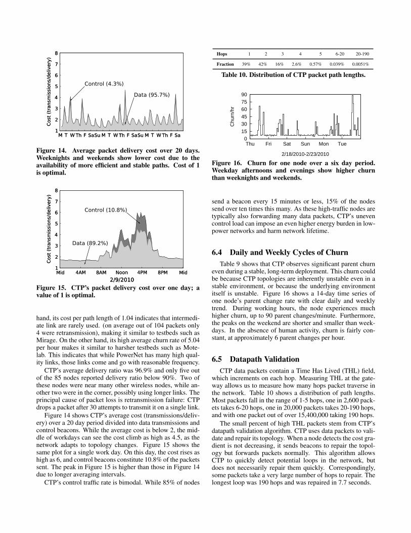
even during a stable, long-term deployment. This churn couldbe because CTP topologies are inherently unstable even in astable environment, or because the underlying environmentitself is unstable. Figure 16 shows a 14-day time series ofone node’s parent change rate with clear daily and weeklytrend. During working hours, the node experiences muchhigher churn, up to 90 parent changes/minute. Furthermore,the peaks on the weekend are shorter and smaller than week-days. In the absence of human activity, churn is fairly con-stant, at approximately 6 parent changes per hour.

6.5 Datapath ValidationCTP data packets contain a Time Has Lived (THL) field,

which increments on each hop. Measuring THL at the gate-way allows us to measure how many hops packet traverse inthe network. Table 10 shows a distribution of path lengths.Most packets fall in the range of 1-5 hops, one in 2,600 pack-ets takes 6-20 hops, one in 20,000 packets takes 20-190 hops,and with one packet out of over 15,400,000 taking 190 hops.

The small percent of high THL packets stem from CTP’sdatapath validation algorithm. CTP uses data packets to vali-date and repair its topology. When a node detects the cost gra-dient is not decreasing, it sends beacons to repair the topol-ogy but forwards packets normally. This algorithm allowsCTP to quickly detect potential loops in the network, butdoes not necessarily repair them quickly. Correspondingly,some packets take a very large number of hops to repair. Thelongest loop was 190 hops and was repaired in 7.7 seconds.

Sequence  Numbers  

Inferred  Losses  Reboot  Beacon  

Figure 17. Visual depiction of CTP link estimation bug.On reboot, the link estimator infers a sequence number0 packet as a long string of failures, raising the link costhigh enough that CTP will not use it.

6.6 Duplicate SuppressionWe find that overall 1.7% of the packets received at the

basestation were duplicates. Packets from eight nodes had aduplication rate above 3.7%. During our 90-day deployment,due to misconfiguration, we deployed two nodes with ID 185in two different areas of the network. The two nodes continueto report readings to the basestation but there are twice asmany packets logged at the server. These packets elude CTPduplicate suppression due to two reasons. First, these twonodes often do not share a path. Second, the packet signatureused for duplicate detection includes node ID, sequence num-ber, and number of hops but the latter two are rarely the samebetween packets of the two nodes.

6.7 Link Estimation BugWe encountered one bug while deploying CTP that existed

in CTP’s four bit link estimator (4B) [12]. We observed thebug during test deployments in December of 2009 and it didnot affect the real 90 day deployment presented here.

The bug occurs when a mote reboots and other motes donot choose the rebooted mote as a next hop for many hours.In the case when the CTP root reboots, this causes the en-tire topology to collapse and encounter the count-to-infinityproblem.

The bug stems from how the link estimator handles bea-con packets. When CTP sends a beacon, the link estimatoradds a header and a variable number of footer entries. Theheader contains a sequence number, so nodes can infer lossesby sequence number gaps. The arithmetic, however, is suchthat if a node reboots and sends sequence number zero, nodesassume that all packets between the last one heard and 0 werelost, as shown in Figure 17. Such a long string of lossescauses the link cost to climb far above the cutoff thresholdCTP will use. The only thing that can bring the link costdown is a long series of received beacons. However, CTP’sadaptive beaconing means that it can take hours to days for along enough sequence.

This bug is not particular to the root. Nodes that rebootwill not be chosen as parents. If a network is dense enough,the removal of one parent does not greatly harm the topol-ogy, as nodes can route around it. It is worth noting that theCTP publication evaluated the effect of node failures on per-formance, but not reboots.

We fixed this bug by capping the number of losses a se-quence number gap can infer to 10. Doing so caps how far inhistory CTP considers sequence numbers, causing it to lendmore weight to the recent reception than the prior losses. In-corporating this fix allows CTP to operate properly in the face

of even somewhat common node reboots. The CTP authorshave incorporated our fix into the standard implementation.

7 DiscussionPowerNet’s extensive power and utilization measurements

reveal how different parts of a computing infrastructure con-tribute to total power cost. This section discusses several ap-proaches which can help reduce power consumption.

7.1 InterventionsWhile energy-efficiency improvements have the great-

est potential to reduce power consumption, educating usersshould not be under-estimated. Section 3 showed that smallchanges in how we use LCD screens can lead to 20% sav-ings. We have found that informing users about the powerdraw of their monitors and giving suggestions on how theycan conserve energy has affected behavior positively.

In the future we anticipate expanding these efforts in sev-eral ways. One is to have an interactive display that allowsbuilding occupants to dig through the data, exploring it in away that interests them. Such engagement with real-worlddata brings attention to energy consumption. In addition, weplan to make individual data available to users who volunteerto participate in the PowerNet monitoring. Power data will al-ways be tied back to utilization to remind people of situationsin which energy is wasted.

7.2 Policy ChangesIn addition to educating individual occupants, our work

has provided insights to the administrative and IT staff in thebuilding. Simply providing detailed data of power usage hasprompted the staff to think about possibilities for savings.

For example, Section 3 briefly mentioned that staff ma-chines are required to be powered on at night so data backupscan complete. These backups can also be observed in Fig-ure 10 by noticing the daily traffic spikes, for example theones shortly after midnight. We learned that different groupsof machines had different start backup times but no machinehad to be on for more than one hour. We pointed out thatpowering staff machines 24-7 was wasteful since they werenever needed for more than approximately 12 hours a day.The suggestion we heard back was that backups could occurduring the lunch hour. Instead, we plan to propose that Wake-on-LAN is used in conjunction with the backup system. Thescripts that currently run can be modified to wake a machinebefore the backup and put it back to sleep one hour later. Thecurrent backup policy is causes at least 30 machines to waste32 kWh every day, costing $130 a month.

7.3 Technical AlternativesBy far, the most effective way to reduce energy consump-

tion of computing systems is to shut them down when theyare not needed. Section 3 showed that personal computersconstitute 16% of the building’s energy consumption, whileSection 4 showed they are rarely used for more than 12 hoursa day. The energy consumption data suggests that turning idle

0 10 20 30 40 50 60Duration of Idle Period (mins)

0

20

40

60

80

100%

Sav

ing

over

Cur

rent

under 5.0% CPU

under 3.0%

under 1.0%

under 0.5%

A

B

C

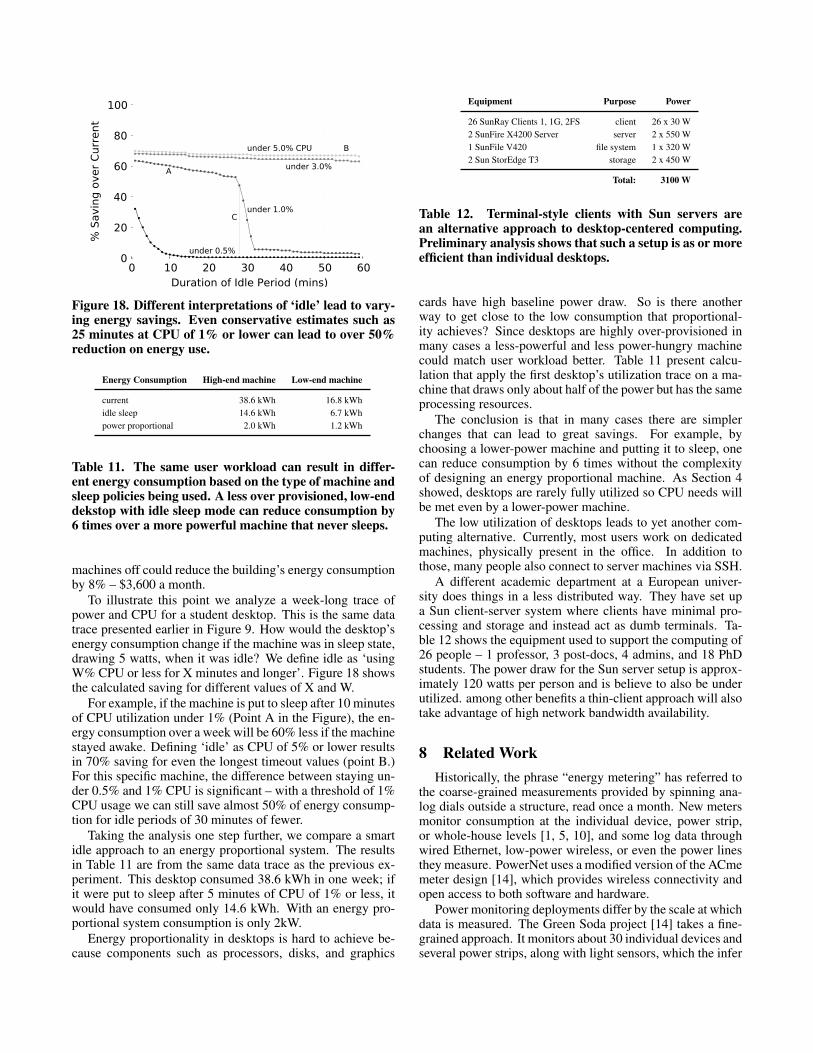
Figure 18. Different interpretations of ‘idle’ lead to vary-ing energy savings. Even conservative estimates such as25 minutes at CPU of 1% or lower can lead to over 50%reduction on energy use.

Energy Consumption High-end machine Low-end machine

current 38.6 kWh 16.8 kWhidle sleep 14.6 kWh 6.7 kWhpower proportional 2.0 kWh 1.2 kWh

Table 11. The same user workload can result in differ-ent energy consumption based on the type of machine andsleep policies being used. A less over provisioned, low-enddekstop with idle sleep mode can reduce consumption by6 times over a more powerful machine that never sleeps.

machines off could reduce the building’s energy consumptionby 8% – $3,600 a month.

To illustrate this point we analyze a week-long trace ofpower and CPU for a student desktop. This is the same datatrace presented earlier in Figure 9. How would the desktop’senergy consumption change if the machine was in sleep state,drawing 5 watts, when it was idle? We define idle as ‘usingW% CPU or less for X minutes and longer’. Figure 18 showsthe calculated saving for different values of X and W.

For example, if the machine is put to sleep after 10 minutesof CPU utilization under 1% (Point A in the Figure), the en-ergy consumption over a week will be 60% less if the machinestayed awake. Defining ‘idle’ as CPU of 5% or lower resultsin 70% saving for even the longest timeout values (point B.)For this specific machine, the difference between staying un-der 0.5% and 1% CPU is significant – with a threshold of 1%CPU usage we can still save almost 50% of energy consump-tion for idle periods of 30 minutes of fewer.

Taking the analysis one step further, we compare a smartidle approach to an energy proportional system. The resultsin Table 11 are from the same data trace as the previous ex-periment. This desktop consumed 38.6 kWh in one week; ifit were put to sleep after 5 minutes of CPU of 1% or less, itwould have consumed only 14.6 kWh. With an energy pro-portional system consumption is only 2kW.

Energy proportionality in desktops is hard to achieve be-cause components such as processors, disks, and graphics

Equipment Purpose Power

26 SunRay Clients 1, 1G, 2FS client 26 x 30 W2 SunFire X4200 Server server 2 x 550 W1 SunFile V420 file system 1 x 320 W2 Sun StorEdge T3 storage 2 x 450 W

Total: 3100 W

Table 12. Terminal-style clients with Sun servers arean alternative approach to desktop-centered computing.Preliminary analysis shows that such a setup is as or moreefficient than individual desktops.

cards have high baseline power draw. So is there anotherway to get close to the low consumption that proportional-ity achieves? Since desktops are highly over-provisioned inmany cases a less-powerful and less power-hungry machinecould match user workload better. Table 11 present calcu-lation that apply the first desktop’s utilization trace on a ma-chine that draws only about half of the power but has the sameprocessing resources.

The conclusion is that in many cases there are simplerchanges that can lead to great savings. For example, bychoosing a lower-power machine and putting it to sleep, onecan reduce consumption by 6 times without the complexityof designing an energy proportional machine. As Section 4showed, desktops are rarely fully utilized so CPU needs willbe met even by a lower-power machine.

The low utilization of desktops leads to yet another com-puting alternative. Currently, most users work on dedicatedmachines, physically present in the office. In addition tothose, many people also connect to server machines via SSH.

A different academic department at a European univer-sity does things in a less distributed way. They have set upa Sun client-server system where clients have minimal pro-cessing and storage and instead act as dumb terminals. Ta-ble 12 shows the equipment used to support the computing of26 people – 1 professor, 3 post-docs, 4 admins, and 18 PhDstudents. The power draw for the Sun server setup is approx-imately 120 watts per person and is believe to also be underutilized. among other benefits a thin-client approach will alsotake advantage of high network bandwidth availability.

8 Related WorkHistorically, the phrase “energy metering” has referred to

the coarse-grained measurements provided by spinning ana-log dials outside a structure, read once a month. New metersmonitor consumption at the individual device, power strip,or whole-house levels [1, 5, 10], and some log data throughwired Ethernet, low-power wireless, or even the power linesthey measure. PowerNet uses a modified version of the ACmemeter design [14], which provides wireless connectivity andopen access to both software and hardware.

Power monitoring deployments differ by the scale at whichdata is measured. The Green Soda project [14] takes a fine-grained approach. It monitors about 30 individual devices andseveral power strips, along with light sensors, which the infer

power consumption of overhead lighting. The Green Sodaproject demonstrated the feasibility of an indoor wirelessmonitoring infrastructure. The similar PowerNet project [15]presents initial insight into the power and utilization of com-puting systems, with mostly wired meters.

PowerNet builds upon the Green Soda and PowerNetprojects in several ways. The system measures more de-vices and a greater variety of computing devices, over a muchlonger time period. The addition of utilization meters enablescorrelated power and utilization measurement, which enablesus to draw conclusions about efficiency, not just the break-down of energy usage. The wireless deployment is unusallydense, and our experiences with its performance and oper-ation can provide guidance for future power monitoring ef-forts, as well as indoor sensor deployments.

Other green computing projects have looked into the chal-lenges of visualizing power data and presenting it to build-ing residents. Energy dashboards [3, 4] and websites [2, 9]summarize and compare power usage data in order to encour-age savings. Many universities have taken advantage of dash-board software to educate students living in dorms, gener-ally with measurements at the granularity of one floor or thewhole building. The Energy Dashboard Project at UCSD [8]covers academic buildings with one to four aggregate me-ters in each building. Such data is useful when comparingpower consumption between buildings and looking for high-level trends in the data. However, aggregate power goes notidentify the parts of the building or the types of devices thatare wasting energy. While not the focus of this paper, Power-Net has also joined in the effort, with a website and display inthe lobby. Unlike other dashboards, ours includes utilizationdata to highlight wasted energy.

9 Conclusion and Future WorkOne over-arching question drove the PowerNet deploy-

ment: how can fine-grained power and utilization data createa high-level, building-scale, actionable understanding of theusage and efficiency of the our computing infrastructure?

The first challenge was that of collecting data – how manyand what type of sensors are needed, and where they shouldgo? Throughout the deployment we learned that wired sen-sors have their place for sparse measurements, but that adense network of open-source wireless sensors avoids the un-expected practical issues of installation and debugging. Wefound that CTP performance degrades during business hours,but provides reasonably high transmission rates and robust-ness for a large deployment in a previously-untested indoorsetting. The current system has collected over 150 gigabytesof data, but is still far from perfect. Future priorities are in-clude adding 300 wireless meters to cover more servers andother equipment, and installing more utilization sensors.

Once fine-grained data is in, the next challenge is to de-rive an accurate breakdown suitable for making high-levelobservations about classes of devices. The aggregate mea-surements of 138 power meters amount to only 2.5% of thebuilding total. However, by learning device totals and distri-butions from other sources, including surveys, observations,and IT database records, then cross-correlating these with

power data, one can construct a reasonably accurate quan-titative breakdown. Precise extrapolation requires knowledgeof how individual devices within a class compare. For ex-ample, desktop power shows high variation, up to 10x, andthus dense instrumentation is needed. On the other hand, net-work power draw is constant over time so only a few sensorreadings suffice.

We find that desktops and servers account for 46% of thebuilding’s electricity consumption, monitors account for 7%,and networks for 3%. While these numbers might differ forother office buildings, our methodology and high-level in-sights will remain valuable. They guide our understandingof how to have meaningful impact on reducing energy con-sumption.

Therefore, the final challenge is turning quantitative anal-ysis into qualitative comparisons, recommendations for com-puter system design – and even purchasing guidelines. Onthis front, we claim no complete answers, only initial insights.The energy breakdown shows where to focus efforts, whilethe correlated power and utilization measurements highlightareas of inefficiency. Specifically, we show that determin-ing idle state and transitioning PCs to a low-power mode canhave a dramatic impact. Another example is monitors; thedata showed a harmless way to save energy. The fact that afew offices have actually our suggstions, resulting in energysavings encourages us to continue building out the deploy-ment and mining the data.

10 References

[1] Arch Rock. www.archrock.com.[2] Google Power Meter. www.google.org/powermeter.[3] Lucid Design Group Building Dashboard.

www.luciddesigngroup.com.[4] Onset Data Loggers. www.onsetcomp.com.[5] Plugwise. www.plugwise.com.[6] RPL: IPv6 Routing Protocol for Low power and Lossy Networks. IETF

Draft, http://tools.ietf.org/html/draft-ietf-roll-rpl-07.[7] TEP 123: Collection Tree Protocol.

http://www.tinyos.net/tinyos-2.x/doc/.[8] UC San Diego Energy Dashboard Project. energy.ucsd.edu.[9] Visible Energy Inc. www.visiblenergy.com.

[10] Watt’s up internet enabled power meters. https://www.wattsupmeters.com/secure/products.php, 2009.

[11] P. Dutta, J. Taneja, J. Jeong, X. Jiang, and D. Culler. A build-ing block approach to sensornet systems. In In Proceedings of theSixth ACM Conference on Embedded Networked Sensor Systems (Sen-Sys’08), 2008.

[12] R. Fonseca, O. Gnawali, K. Jamieson, and P. Levis. Four-bit wirelesslink estimation. In Hotnets-VI, Atlanta, GA, 2007.

[13] J. W. Hui and D. Culler. The dynamic behavior of a data disseminationprotocol for network programming at scale. In Proceedings of the Sec-ond International Conferences on Embedded Network Sensor Systems(SenSys), 2004.

[14] X. Jiang, S. Dawson-Haggerty, P. Dutta, and D. Culler. Design andimplementation of a high-fidelity ac metering network. In Proceed-ings of The 8th ACM/IEEE International Conference on InformationProcessing in Sensor Networks (IPSN ’09), San Francisco, CA, USA.

[15] M. Kazandjieva, B. Heller, P. Levis, and C. Kozyrakis. Energy dump-ster diving. In Workshop on Power Aware Computing and Systems(HotPower’09), 2009.