IDENTIFICATION OF VORTEX STRUCTURES IN …vm.tstu.tver.ru/topics/publications/ISFV15-090.pdf · identification of vortex structures in transitional free-convection boundary layer

15th International Symposium on Flow Visualization June 25-28, 2012, Minsk, Belarus

ISFV15 – Minsk / Belarus – 2012

IDENTIFICATION OF VORTEX STRUCTURES IN TRANSITIONAL FREE-CONVECTION BOUNDARY LAYER USING DATA OF

TEMPORAL DIRECT NUMERICAL SIMULATION

A.G. ABRAMOV1, E.M. SMIRNOV1,c, V.D. GORYACHEV2

1Department of Aerodynamics, St.-Petersburg State Polytechnic University, St.-Petersburg, 195251, Russia 2Department of Mathematics, Tver State Technical University, Tver, 170026, Russia

cCorresponding author: Tel.: +78122972419; Fax: +78125526621; E-mail: [email protected]

KEYWORDS: Main subjects: laminar-turbulent transition, heat transfer, flow visualization

Fluid: free convection of air along a hot vertical plate Visualization method(s): computer visualization of numerical data Other keywords: direct numerical simulation, vortex structures

ABSTRACT: The present contribution is aimed at graphic post-processing of direct numerical simulations (DNS) data

obtained for time-developing air free convection assuming periodicity conditions in both the direction parallel to the vertical isothermal hot plate. The flow visualization is performed with the in-house software HDVIS being under development to provide the user with advanced tools for visual analysis of data after 3D steady/unsteady flow simulation. HDVIS possibilities for identification of various vortex structures are illustrated first for two cases of the Rayleigh-Bénard convection. For the free-convection boundary layer, a special attention is paid to 3D vortex structures that occur at the non-linear stage of 2D laminar flow destruction and clearly manifest themselves up to the end stage of laminar-turbulent transition in the layer. Effects of initial isotropic disturbances imposed in the flow domain on transition are discussed.

1. INTRODUCTION The turbulent air free-convection boundary layer (BL) along a vertical hot flat plate is a classical example of

thermally driven flow and was investigated intensively both experimentally [1-5] and numerically [6-8]. Much less attention was paid to transition phenomena in this type of flow despite in many cases the transition region can occupy a considerable part of the vertical surface with a developing boundary layer. Moreover, transitional Rayleigh numbers, based on the distance from the plate edge, differ considerably in various experiments [3-5], and the reasons of that remains to be questionable. From the general position, it points to the necessity of research work on the problem of receptivity of the developing free-convection boundary layer to external disturbances of various kinds and scales. As a part of this research work, studies aimed at discovering and classification of eigen non-linear modes of disturbances in the BL are of special importance.

The colossal progress in performance of computer cluster systems and developments of advanced parallel CFD-solvers have offered the prospect of wide-ranging numerical studies of transitional and turbulent convection flows on the base of 3D unsteady formulations. Direct Numerical Simulation (DNS) is the most attractive and reliable approach for getting a detailed knowledge on convection. However, traditional, "spatial" DNS approach assuming full modeling of spatial-temporal development of free-convection boundary layer remains to be extremely time-consuming. Time-developing (Temporal) DNS technique (TDNS) allows reducing computational efforts significantly, and can provide valuable information for getting more insights into peculiarities of this type of flows and associated heat transfer phenomena [9, 10]. The TDNS approach is based on substitution of flow development in space by its temporal evolution, i.e. time plays here a role of coordinate in the main flow direction.

The present work covers results of visual post-processing of the time-developing DNS data obtained in [10] for the air free-convection flow near a vertical isothermal hot plate. The main aim is identification and analysis of vortex structures at transitional studies of the boundary layer developing in time under influence of initial disturbances introduced into the computational domain. As well, possibilities of the in-house software HDVIS used for advanced graphic post-processing are described and illustrated.



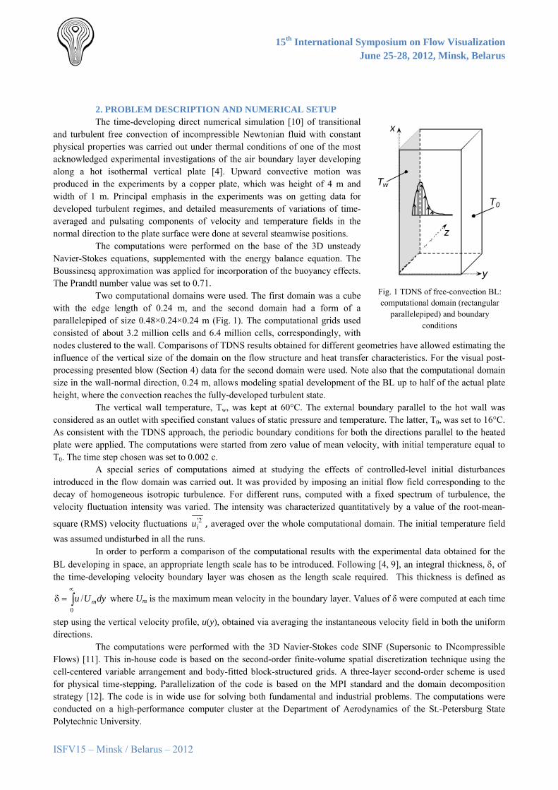
2. PROBLEM DESCRIPTION AND NUMERICAL SETUP The time-developing direct numerical simulation [10] of transitional

and turbulent free convection of incompressible Newtonian fluid with constant physical properties was carried out under thermal conditions of one of the most acknowledged experimental investigations of the air boundary layer developing along a hot isothermal vertical plate [4]. Upward convective motion was produced in the experiments by a copper plate, which was height of 4 m and width of 1 m. Principal emphasis in the experiments was on getting data for developed turbulent regimes, and detailed measurements of variations of time-averaged and pulsating components of velocity and temperature fields in the normal direction to the plate surface were done at several steamwise positions.

The computations were performed on the base of the 3D unsteady Navier-Stokes equations, supplemented with the energy balance equation. The Boussinesq approximation was applied for incorporation of the buoyancy effects. The Prandtl number value was set to 0.71.

Two computational domains were used. The first domain was a cube with the edge length of 0.24 m, and the second domain had a form of a parallelepiped of size 0.48×0.24×0.24 m (Fig. 1). The computational grids used consisted of about 3.2 million cells and 6.4 million cells, correspondingly, with nodes clustered to the wall. Comparisons of TDNS results obtained for different geometries have allowed estimating the influence of the vertical size of the domain on the flow structure and heat transfer characteristics. For the visual post-processing presented blow (Section 4) data for the second domain were used. Note also that the computational domain size in the wall-normal direction, 0.24 m, allows modeling spatial development of the BL up to half of the actual plate height, where the convection reaches the fully-developed turbulent state.

The vertical wall temperature, Tw, was kept at 60°C. The external boundary parallel to the hot wall was considered as an outlet with specified constant values of static pressure and temperature. The latter, T0, was set to 16°C. As consistent with the TDNS approach, the periodic boundary conditions for both the directions parallel to the heated plate were applied. The computations were started from zero value of mean velocity, with initial temperature equal to T0. The time step chosen was set to 0.002 с.

A special series of computations aimed at studying the effects of controlled-level initial disturbances introduced in the flow domain was carried out. It was provided by imposing an initial flow field corresponding to the decay of homogeneous isotropic turbulence. For different runs, computed with a fixed spectrum of turbulence, the velocity fluctuation intensity was varied. The intensity was characterized quantitatively by a value of the root-mean-

square (RMS) velocity fluctuations 2'iu , averaged over the whole computational domain. The initial temperature field

was assumed undisturbed in all the runs. In order to perform a comparison of the computational results with the experimental data obtained for the

BL developing in space, an appropriate length scale has to be introduced. Following [4, 9], an integral thickness, δ, of the time-developing velocity boundary layer was chosen as the length scale required. This thickness is defined as

∫∝

=δ0

/ dyUu m where Um is the maximum mean velocity in the boundary layer. Values of δ were computed at each time

step using the vertical velocity profile, u(y), obtained via averaging the instantaneous velocity field in both the uniform directions.

The computations were performed with the 3D Navier-Stokes code SINF (Supersonic to INcompressible Flows) [11]. This in-house code is based on the second-order finite-volume spatial discretization technique using the cell-centered variable arrangement and body-fitted block-structured grids. A three-layer second-order scheme is used for physical time-stepping. Parallelization of the code is based on the MPI standard and the domain decomposition strategy [12]. The code is in wide use for solving both fundamental and industrial problems. The computations were conducted on a high-performance computer cluster at the Department of Aerodynamics of the St.-Petersburg State Polytechnic University.

Tw

T0

x

y

z

Fig. 1 TDNS of free-convection BL: computational domain (rectangular

parallelepiped) and boundary conditions



3. VISUALIZATION TOOL. EXAMPLES OF VISUALIZATION OF CONVECTIVE FLOWS Success in application of visualization techniques for getting a deep understanding of one or other type of

unsteady convective flows is dependent on possibilities to perform an interrelated analysis of spatially extended and time-developing vortex systems. Customary practice of using velocity vector fields in chosen sections results often in an incomprehensible picture of partly intersected arrows befogged by occlusions effects. As a rule, appropriate sections for visualization are poorly predictable, and choice of a proper view direction on vortex structures of complicated forms is a time-consuming process. A preferable way consists in performing additional post-processing calculations followed by creation of geometrical objects for secondary fields (derived quantities) such as functionally colored stream surfaces, isosurfaces of derived quantities, virtual flow particle paths etc. Flow structure identification can be Eulerian, concerned with quantities derived from the instantaneous velocity field and its gradient. Structure criteria formulated in terms of the invariants of the velocity gradient tensor, the Q-criterion and the swirling strength criterion λ2 [13, 14] are especially often used in vortex structure identification. They promote to extract flow regions where rotation dominates over strain. Alternative (and/or additional) method of identifying flow structures is Lagrangian, it is based on the tracing of fluid particle trajectories.

On-the-fly calculation of derived vorticity and tensor fields, stream and streak lines, generation of proper geometrical objects and their ray tracing with a huge amount of data are very computationally expensive. Consequently, an advanced visual treatment of complicated flow fields requires parallel possibilities of visualization software.

The above characterized visualization techniques and algorithms required are realized in the in-house system HDVIS (High Definition VISualization) being under development for several last years [15]. This tool was used for graphic post-processing of the TDNS data for the free-convection BL, and results of this work are given in the next Section. In the present Section, HDVIS possibilities for identification of various vortex structures are illustrated after post-processing of numerical data obtained earlier [16, 17] for two problems of the Rayleigh-Bénard (RB) convection.

The first problem is mercury convection in a confined cylindrical cell of the aspect ratio of 1 heated from below (Fig. 2). The second problem is thermal convection in a horizontal layer under the influence of rapid rotation which includes important phenomena related to geophysical and astrophysical flows. These problems, considered in the non-dimensional form, were numerically investigated using also the code SINF. Note that turbulence modeling of high-Ra regimes of convection was performed with an eddy-resolving approach (a kind of RANS/LES hybridization) involving the transport equation for the unresolved motion kinetic energy [16].

The numerical simulations of the RB mercury convection (Pr = 0.025) were performed for the Rayleigh number (Ra) ranging from 106 to 5×109 under conditions of the experiments [18] and DNS [19]. Some results of flow

Fig. 2 Visualization of turbulent Rayleigh-Bénard mercury convection in a confined cylindrical cell at (a-b) Ra = 106 and (c) Ra = 108: (a) – isosurfaces of vertical velocity w = ±0.25; (b) – temperature isosurface T = 0.42 (green) and isosurfaces of Q-criterion equal to 100, mapped by local temperature; (c) – temperature isosurfaces T = 0.25 (blue), 0.5 (pink), 0.75 (red), streamlines around a

vortex in the flow core, and temperature distribution near the top wall created with a local color palette (0 ≤ T ≤ 0.25)

a



visualization are given Figs. 2, 3. The complicated turbulent convection developing in the cell is characterized by formation of a stable large-scale circulation that spans the whole height of the enclosure. The presence of this global circulation is illustrated in Fig. 2a by the means of two isosurfaces of the vertical velocity corresponding to the absolute value of 0.25. Note that the global structure changed slowly its orientation in time that could be quite expected due to the axial symmetry of the cell. A "swan-neck" temperature isosurface shown in Fig. 2b divides conventionally on the cold and the hot flow regions. Isosurfaces of Q-criterion point to presence of concentrated vortices developed on the periphery of the cell at a moderate value of the Rayleigh number (Fig. 2b). At higher Ra-values, the flow core is occupied by vortices of various orientations (Fig. 2c). Remarkably that even a proper temperature isosurface, T=0.5, gives an evidence of presence of intensive vortices in the flow core at Ra = 108. Due to formation of multiple vortex structure, instantaneous heat flux distributions over the isothermal top and bottom of the cell are strongly nonuniform. For the top, it can be seen from the temperature map given in Fig. 2c for the plane that is 2.65·10-4 apart of the wall.

Another prominent feature of the turbulent RB convection appears distinctly for high-Ra regimes is associated with vertical movement of fluid portions (thermal plumes). The plumes were detected via observation of instantaneous temperature field in the vicinity of the isothermal walls as it is illustrated in Fig. 3 for the near-bottom region. Strong turbulent mixing in the flow core as demonstrated clearly in Fig. 2c by the isotherm T = 0.5 prevents thermals to move through the central part of the cell. As a result, most of thermals are localized near the lateral walls including regions of rising and descending large-scale motion. Thermal plumes affect in turn the global circulation and lead to certain smoothing of horizontal inhomogeneity of temperature field.

Rapidly rotating convection at Pr = 1 was simulated for a horizontal layer heated from below. The fluid layer was bounded at the top and bottom by plane walls kept at fixed temperatures and rotating about a vertical axis with constant angular velocity. Applying periodicity conditions in both the horizontal directions, the computations were performed for the Rayleigh number Ra ≈ 108, and the Rossby number, Ro, equal to 0.75, this set corresponds to one of the regimes examined in a previous DNS study [20]. The structure of the convection simulated is illustrated in Fig. 4.

Fig. 4 Visualization of turbulent RB convection in a rapidly rotating horizontal layer at Ra = 106 and Ro = 0.75: (a) streamlines patterns combined with isosurfaces of Q = 6 colored by local temperature; ( b) isosurfaces Q = 2 colored by temperature, streamlines

in a plane near the top wall colored by normalized local velocity, and temperature distributioin over a plane near the bottom wall

-0.010 0.005 0.020 0.035 0.050v

Fig. 3 Thermal plumes in RB mercury convection: temperature isosurface (T = 0.9) colored by vertical velocity (Ra = 8.7·108)

ba



1

10

100

104 105 106 107 Gr

Nu- experiments [4]- TDNS [9]- present computations

1E-005 0.0001 0.001 0.010.0

1.0

2.0

3.0

0.0 2.0 4.0 6.0 8.00

100

200

300

400

5000.0 2.0 4.0 6.0 8.0

0.00

0.04

0.08

0.12

0.16

xcr

q [W/m2]

[m]

t [s]

increase of 2'u

t [s]

(a)

(b)

(c)1

23

2'u [m2/s2]

increase of 2'u

0.01 0.1 1 100

0.2

0.4

0.6

0.8

1

0.01 0.1 1 100.00

0.05

0.10

0.15

0.20

y/

u/Um

TT 2'

∆

T

y/

(d)

(e) (f)

δ

δ δ

δ

δ

Fig. 5 (a-c) Effect of controlled initial disturbances on laminar-turbulent transition position in the free-convection BL, (d) Nusselt vs Grashof numbers in comparison with experimental [4] and TDNS [9] data, (e,f) comparison of (lines) the computer-generated

profiles of the averaged and pulsating field quantities with (symbols) the results of experiments [4]

Combination of 3D streamlines patterns with isosurfaces of Q = 6 in Fig.4a gives a clear image of the convection with many cyclonic vortices, and points that the cores of these vortices are of mainly vertical orientation. The 2D streamline pattern in Fig. 4b illustrates formation of a number of vortex-sink flows in the vicinity of the wall, with a separatrix manifold. The general 3D image of the rotating RB convection given in Fig. 4b was created using a special graphic processing of isosurfaces of the Q-criterion set to 2. Nevertheless, even so advanced "static" pictures do not provide full understanding of spatial-temporal dynamics of the convection considered and an advanced flow animation is needed additionally.

4. FREE-CONVECTION BOUNDARY LAYER: RESULTS AND DISCUSSION

4.1. Effect of initial disturbances on laminar-turbulent transition. Comparison with experiments for turbulent regime

As mentioned in Section 2, a series of computations was carried out for different intensity of initial velocity fluctuations in order to study the effect of controlled-level disturbances on laminar-turbulent transition in the free-convection BL along the vertical hot plate. A run with no initial disturbances imposed was done as well.

Fig. 5a shows time dependences of the integral thickness δ for three runs with different values of initial velocity fluctuation intensity (marked with numerals in Fig. 5c). For each case, one can clearly see a moment of a sharp change in the δ growth rate, corresponding to onset of laminar-turbulent transition. For the same runs, time evolution of the surface-averaged wall heat flux is given in Fig. 5b. With these curves, the transition onset can be easily identified as well.

In order to determine critical values of the local Grashof number, Grx, a preliminary calculation of spatial development of a 2D steady laminar free-convective BL was done under the same thermal conditions. It has provided a dependence of δ(x), which was applied to data in Fig. 5a to define for each run a critical value of the longitudinal coordinate. Transition onset positions, xcr, defined for different computational runs are given in Fig. 5c in the form of

dependency on 2'iu . Note that the experimental value xcr ≈ 0.7 m [4]. It is seen that in the no-initial-disturbances case a

significant delay of the transition takes place (xcr ≈ 3.2 m). With imposing initial disturbances of an increasing intensity, the transition position coordinate first shifts rapidly to the lower edge of the plate, and then stabilizes approaching to the



Fig. 6 Evolution of vortex structures in the time- developing free-convection boundary layer visualized by isosurfaces of Q = 10 s-2 colored by steamwise velocity: (left to right) t = 0.4, 0.8, 1.2, 1.6, 2.0 s

experimental value. Computations of temporal development of convection with a specified level of initial disturbances have

allowed obtaining a good agreement with the experimental data [4] and the TDNS results [9], including the relation between the Nusselt and the Grashof number, both based on the integral thickness (Fig. 5d). For a particular time instant, when the computed value of δ was equal to the experimental one defined for the measurement section of x ≈ 1.44 m [4], a comparison of numerically predicted and measured profiles of mean temperature, mean vertical velocity and fluctuation characteristics of the turbulent convection was performed. As shown in Fig. 5(e, f), being presented in a non-dimensional form, the profiles agree rather satisfactorily with the experimental data, like that reported in [9]. It has to be noted, however, that the dimensional value of the maximum mean velocity computed is over-predicted by about 30%.

4.2. Visualization and analysis of evolving flow fields Several visualization techniques were applied to hightlight various aspects of vortex structure identification

in the free-convection boundary layer BL devolping in time near a heated vertical plate. As a primary techique, creation of geometrical objects associated with Q-criterion isosurfaces was chosen after an expierance accumulated previously. Setting various values of the Q-criterion, one is able to focus upon different pecularities of the convection under analysis.

For five time instants, Figure 6 presents isosurfaces for a relatively low value of the Q-criterion (Q=10 s-2). Generally, this value is not enough to extract concetrated vortices but nevertheless various non-linear stages of 2D laminar flow destruction is clearly seen. Remarkably, that for the first of the time instants visualized, t = 0.4 s, the Q-isosurfaces shows mainly remains of initial disturbances. Note that in Fig. 6 and hereinafter numerical data obtained

with 2'iu =4.9·10-4 m2/s2 is visualized. A special interest in Fig. 6 is caused by the image created for t = 1.2 s. Here

development of "eigen" 3D modes of the transitional boundary layer is clearly seen. Note that at the first look this image can lead to a wrong conclusion for opposite directions of fluid particle rotation in the high-velocity (orange) and low-velocity (blue) parts of typical large-scale configurations forming in the layer. Another image of such a configuration given in Fig. 7 points that the high-velocity region of the "eigen" mode does not possess vorticity that is considerably higher than the laminar layer vorticity. Contrary to that, the low-velocity part, belonging to the our part of the BL, can be started to characterized as a concentrated vortex.

Figure 8 presents isosurfaces for a higher value of the Q-criterion (Q=200 s-2). Here formation of concentrated hairpin-like vortices occupying with time increase larger and larger parts of the BL is clearly seen. Remarkably that the head of the "harpins" is inclined opposite to the main flow direction. Instant distributions of wall



heat flux over the plate surface shown in Fig. 8 point clearly that the vortices developing has a srong effect on local heat transfer to the plate.

Impressive images of the concentrated vortices developing in the outer part of the boundary layer are given in Fig. 9 for t = 1.6 and 2.0 s. Isosurfaces of the Q-criterion for the larger time were created setting Q = 600 s-2, and clearly represent the form of the vortex core.

Numerical schlieren technique was also applied to visualize the transitional processes in the free-convection boundary layer simulated (Fig. 10). The pictures created reflect a generic structure of convection, effect of developing vortices on the temperature gradients etc. Note that the color "veins" seen in the graphs given in Fig. 10 are remains of Q-criterion isosurfaces cut by the planes used to extract data for numerical schlieren. One more technique applied consists in creation of band-like fragments of a Q-criterion isosurface by cutting the whole surface with two parallel vertical planes normal to the heated plate. Projections of these "bands" onto the normal plane shown in Fig. 11 give 2D images of

instabilities developing in the boundary layer. As a next step of the present investigations, preliminary numerical simulation of laminar-turbulent transition

in the free-convection boundary layer was carried out on the base of SDNS approach. Here, the computational domain used had the form of a parallelepiped of 1.92×0.24×0.24 m in size. The computational grid consisted of about 26 million cells keeping basic parameters of the grids used in the TDNS. Periodic boundary conditions were imposed only in the transversal coordinate and the horizontal boundaries considered as an outlet, with possibility of inlet flow. Computations were started from a disturbed velocity field that allowed getting a very good agreement with the experimental data [4] at a certain time interval (including the transition position and the averaged and pulsating characteristics of velocity and temperature fields for a turbulent regime of convection). The main reason of such an improvement in the computational results is connected with reproducing the effect of entrainment of the surrounded cold air by the developing BL (this effect is omitted in the TDNS approach). Remarkably also that the flow visualization performed has discovered the same peculiarities of the flow related to development of "eigen" modes in the form of hairpin vortices. Despite a relative success, the computational setup used for the preliminary SDNS suffers a shortcoming manifesting itself in washing (in time) the initial disturbances imposed out from the computational domain. So it is required to develop a proper method for definition/keeping of prescribed disturbances at inlet boundaries of the domain.

Fig. 8 Evolution of vortex structures in the boundary layer visualized by isosurfaces of Q = 200 s-2: (left to right) t = 1.4, 1.6, 2.0 s. Distibutions of wall heat flux over the plate surface are shown as well.

Fig. 7 An extending representation of flow in the region occupated by

isosurface of Q=10 s-2



Fig. 10 Visualization of different stages of laminar-turbulent transition in the BL by numerical schlieren: (left to right) t = 0.4, 0.6, 0.8, 1.0, 1.2, 1.6, 1.8, 2.0 s

Fig. 11 2D images of the BL transition process created via projections of band-like Q-value-isosurface fragments onto a normal vertical plane (see legend in Fig. 10)

Fig. 9 Visualization of concentrated vortices developing in the BL by (left) t = 1.6 s and (right) t = 2.0 s. Isosurfaces of Q =200 and 600 s-2 colored by vertical velocity are shown for t = 1.6 and 2.0 s respectively



CONCLUSIONS An extensive graphic post-processing of numerical data available for time-developing free-convection

boundary layer has been carried out with an advanced in-house visualization tool. The numerical data used for visual analysis of laminar-turbulent transition peculiarities was generated on the base of the temporal direct numerical simulation. Using various visualization techniques based mostly on calculation and graphic processing of different secondary/derived quantity fields, a significant progress has been achieved in identification and analysis of 3D vortex structures developing in free-convection boundary layers at various studies of transition.

ACKNOWLEDGEMENTS Authors would like express their thanks to Russian Foundation for Basic Research (RFBR) for support of the

work under grants #11-08-00590 and #11-07-00135.

REFERENCES 1. Cheesewright R. Turbulent natural convection from a vertical plane surface. Int. J. Heat Transfer. 1968, 90, p. 1 2. Warner C.Y., Arpaci V.S. An Experimental Investigation of Turbulent Natural Convection in Air along a Vertical Heated Flat Plate. Int. J. Heat Mass Transfer. 1968, 11(3), p. 397 3. Pirovano A. et al. Convection naturelle en regime turbulent le long d’une plaque plane vertical. Proc. 9th Int. Heat Transfer Conf., Paris, France, 1970, 4, NC 1.8, p. 1 4. Tsuji T., Nagano Y. Characteristics of a turbulent natural convection boundary layer along a vertical flat plate. Int. J. Heat Mass Transfer. 1988, 31(8), p. 1723 5. Chumakov Y.S. Temperature and velocity distributions in a free-convection boundary layer on a vertical isothermal surface. High Temperature. 1999, 37, p. 714 6. To W.M., Humphrey J.A.C. Numerical simulation of buoyant, turbulent flow - I. Free convection along a heated, vertical, flat plate. Int. J. Heat Mass Transfer. 1986, 29(4), p. 573 7. Henkes R.A.W.M., Hoogendoorn C.J. Comparison of turbulence models for the natural convection boundary layer along a heated vertical plate. Int. J. Heat Mass Transfer. 1989, 32(1), p. 157 8. Yan Z.H., Nilsson E.E.A. Large eddy simulation of natural convection along a vertical isothermal surface. Heat Mass Transfer. 2005, 41, p. 1004 9. Abedin M.Z. et al. Direct numerical simulation for a time-developing natural-convection boundary layer along a vertical plate. Int. J. Heat Mass Transfer. 2009, 52, p. 4525 10. Abramov A.G. et al. Direct numerical simulation of turbulent time-developing free convection along a heated vertical wall. Proc. of PAVT-2011, Moscow, Russia, 2011 (in Russian) 11. Smirnov E.M., Zaitsev D.K. The finite-volume method in application to complex-geometry fluid dynamics and heat transfer problems. Scientific-Technical Bulletin of the St.-Petersburg State Technical University, 2004. 2(36), p. 70 (in Russian) 12. Smirnov E.M. et al. DNS and RANS/LES-computations of complex geometry flows using a parallel multiblock finite-volume code. In.: Parallel CFD: Advanced Numerical Methods Software and Applications, Elsevier, 2004, p. 219 13. Hunt J.C.R. et al. Eddies, stream, and convergence zones in turbulent flows. Proc. of the Summer Program, Center for Turbulence Research, NASA Ames/Stanford Univ., 1988, p. 193 14. Green M. et al. Detection of Lagrangian coherent structures in three-dimensional turbulence. J. Fluid Mech. 2007, 572, p. 111 15. Zaitsev D.K. et al. Visual analysis of turbulent whirl over a cantilevered flexible blade after 3D numerical simulation. Proc. of ISFV13, Nice, France, 2008 16. Abramov A.G. et al. Numerical study of high-Ra Rayleigh-Bénard mercury and water convection in confined enclosures using a hybrid RANS/LES technique. Proc. of the Eurotherm Seminar 74, Eindhoven, the Netherlands, 2003, p. 33 17. Abramov A.G., Smirnov E.M. Numerical simulation of turbulent thermal convection in confined enclosures on the base of three-dimensional unsteady formulations. Proc. of XVI School-Seminar of Young Scientists and Specialists under the leadership of RAS academician, professor A.I. Leontiev, 2007, Publishing House MPEI, 1, p. 43 (in Russian) 18. Cioni S. et al. Strongly turbulent Rayleigh-Bénard convection in mercury: comparison with results at moderate Prandtl number. J. Fluid Mech., 1997, 335, p. 111 19. Verzicco R., Camussi R. Transitional regimes of low-Prandtl thermal convection in a cylindrical cell. Phys. Fluids. 1997, 9(5), p. 1287 20. Julien K. et al. Rapidly rotating turbulent Rayleigh-Benard convection. J. Fluid Mech. 1996, 322, p. 243

Documents

IDENTIFICATION OF VORTEX STRUCTURES IN …vm.tstu.tver.ru/topics/publications/ISFV15-090.pdf · identification of vortex structures in transitional free-convection boundary layer