Embed Size (px)
Citation preview

IDENTIFICATION OF SYSTEM DYNAMICSUSING MULTIPLE INTEGRATIONS
William Richard Hansell

United StatesNaval Postgraduate School
mT-f jFH ft ft
IDENTIFICATION OF SYSTEM DYNAMICS
USING MULTIPLE INTEGRATIONS
by
William Richard Hansell
Thesis Advisor George J. Thaler
June 1971
/ /?C7?-<?
Approved fioA puhtlc n.al<LCi^&} dd>&UbuutLon untunltzd.
\


Identification of System Dynamics
Using Multiple Integrations
by
William Richard.HansellEnsign, United States Navy
B.E., Villanova University, 1970
Submitted in partial fulfillment of therequirements for the degree of
MASTER OF SCIENCE IN ELECTRICAL ENGINEERING
from the
NAVAL POSTGRADUATE SCHOOLJune 1971
/?

tlfifiASX
IAVAL POSTGRADUATE SCHOOLKMfTSREY. CALIF. 93940
ABSTRACT
A practical method for identifying linear time in-
variant systems on the basis of arbitrary input-output
records is reviewed and extended to handle the case where
the system is not initially in the zero state. The method
is implemented using a digital computer program composed
of a numerical integration subroutine and a subroutine for
solving overdetermined sets of linear algebraic equations.
Several examples are presented to demonstrate the accuracy
and present capabilities of the procedure.


TABLE OF CONTENTS
I. INTRODUCTION 5
A. THE IDENTIFICATION PROBLEM 5
B. OBJECTIVES OF THIS PAPER 9
II. IDENTIFICATION BY MULTIPLE INTEGRATIONS 11
A. GENERAL APPROACH 11
B. IDENTIFYING INITIAL CONDITIONS 17
C. SIMPLIFICATIONS WITH ZERO INITIAL CONDITIONS - 19'
III. IMPLEMENTATION 21
A. NUMERICAL METHODS 21
B. CHARACTERISTICS. OF GOOD INPUT-OUTPUT RECORDS - 22
C. PROGRAM DESCRIPTION 24
D. EXAMPLES 26
IV. CONCLUSIONS 75
COMPUTER PROGRAM 7 7
BIBLIOGRAPHY 97
INITIAL DISTRIBUTION LIST 100
FORM DD 1473 101


ACKNOWLEDGEMENT
The author wishes to express his appreciation to
Doctor George J. Thaler of the Electrical Engineering
Department of the Naval Postgraduate School for the
guidance and helpful suggestions in the preparation of
this work.

I. INTRODUCTION
A. THE IDENTIFICATION PROBLEM
In order to apply any of the modern techniques of
control system design one must first have a mathematical
model of the system to be controlled. The form of this
model will depend on the design methods to be employed as
well as on the physical characteristics of the system.
Since most of the theory on the analysis and design of
control systems is based either on the state space or
transform representation of systems the vast majority of
mathematical models will consist of either a set of state
equations or a transfer function.
v_c Xc ilao DCCii uc^iaou ivnat uabi»- loilu cil<^ ma l-h<
matical model should take the problem of determining the
numerical values o-f the parameters arises. Parameter
values can often be determined from the laws of physics
and the data supplied by a manufacturer or obtained through
testing. This is not always the case however. Occasionally
the laws of physics become mathematically intractable or
are not even applicable. Quite often the values of certain
key parameters are not available. It is in these cases
that the identification problem arises.
A common problem in engineering is that of determining
the output of a system based on a knowledge of the system
model, input, and initial conditions. The identification
problem is similar to this but here the unknown quantity is

the system model. The input and output are assumed to be
known. For the purposes of this thesis the identification
problem can be stated as follows:
Given - a record of the input and output of a system
over some finite period of time,
Find - a mathematical model and the numerical values
of the model parameters in such a way that the
model will accurately describe the behavior
of the system.
It should be kept in mind that the problem of identi-
fying a system solely on the basis of input and output data
(the so called "black box" problem) is very rare in engi-
neering. Even in the case where none of the model parame-
ters are known one will more than likely have a fair idea
of whether the system is linear or nonlinear, time varying
or time invariant, what the order of magnitude of the domi-
nant time constants is, and what types of inputs and out-
puts are to be expected. For this reason most engineering
identification problems fall into the "grey box" category.
This distinction may seem trivial but virtually all iden-
tification techniques rely heavily on knowledge of the
characteristics and quantities mentioned above.
Although the control systems literature on system
identification is quite vast there are no known identifica-
tion schemes capable of handling all identification prob-
lems effectively. Choosing a method suitable for a given
problem can become a formidable task. A paper summarizing

most of the common approaches to the problem of identifying
lumped parameter systems has been published by Nieman,
Fisher, and Seborg [1] . A good discussion of the indus-
trial applications of various methods has been published
by Eykhoff, et al . [2].
One common approach used in linear system identifica-
tion is that of obtaining the impulse response of the sys-
tem. Mishkin and Haddad [3] have developed a technique
for finding the impulse response based on samples of the
system output and its derivatives. A technique for esti-
mating the impulse response on the basis of noisy input and
output samples has been developed by Levin [4] and Kerr and
Surber [5]. Turin [6] and Lichtenberger [7,8] have used a
matched rixter to outain an iuentiiication. iiic use Ox a
white noise or binary test signal and crosscorrelation has
been suggested by Hill and McMurtry [9]. The noise limita-
tions of the sample approximation, matched filter, and
crosscorrelation identification techniques have been in-
vestigated by Lindenlaub and Cooper [10].
Another common approach to the identification problem
is to determine the coefficients of the differential or
difference equation which describes the system. Kumar and
Sridhar [11] have employed the method of quasilinearization
with some success. -Nagumo and Noda [12] have developed a
learning approach to the problem.' Bass [13] has developed
a method which uses modulating functions and works well in
the presence of noise. Astrom and Bohlin [14] have developed

a statistically optimal method of determining differential
equation parameters known as the "maximum likelihood method."
A similar method which is not optimal but is considerably-
simpler computationally has been developed by Peterka and
Smuk [15,16]. It is known as the "prior knowledge fitting
method." An algorithm for determining state variable models
of sampled data systems has been proposed by Ho and Kalman
[17] . The algorithm performs quite well in the presence
of noise, and has been extended to continuously operating
systems by Eldem [18]
.
Methods of identifying nonlinear and distributed param-
eter systems are usually limited to specific types of sys-
tems or to specific types of nonlinearities . This is
unuoubtculy uue to tjie wiu.e variety Oi nonlinearities en-
countered in physical systems and the difficulty of finding
a model capable of characterizing them all. Shinbrot [19],
Mowery [20], Fairman [21], and Bellman, et al . [22] have
all approached the problem of identifying nonlinear systems
by assuming a particular form of differential equation is
capable of describing the system and then developing methods
around the form of differential equation chosen. Another
common approach to nonlinear system identification is that
of representing a system by a suitable functional polyno-
mial relating the input and output. Hsieh [23] uses this
approach and a steepest descent algorithm to solve the iden-
tification problem. Similar approaches have been taken by
Simpson [24], Bose [25,26], and Hubbell [27].
8


Identification methods vary widely with respect to how
much must be known about the system before the method can
be applied. Some identification techniques require that
prior estimates of all system parameters be available.
Many methods restrict the allowable system inputs to a
family of testing functions such as steps or binary pulses.
In general, the less that is known about a given system and
the tighter the constraints on the kind of signals which
may be applied as inputs the more difficult it is to find
a method capable of accomplishing the identification.
B. OBJECTIVES OF THIS PAPER
This paper will present a study of an identification
technique originally suggested by Diamessis [28]. It is
designed to identify lumped linear time invariant systems
but has been extended by Diamessis [29] and Wang [30] to
handle certain types of nonlinearities . The technique re-
quires a knowledge of the system input and output over some
finite time interval as well as a rough estimate of the sys
tern order. The system input need not be restricted to a
class of testing functions, it can be completely arbitrary.
Unlike some identification techniques which require
the calculation of derivatives of the input and output, the
technique to be presented requires only integrals of the
input and output. The advantages of numerical integration
over differentiation are well known. Since any zero mean
noise component on the input or the output tends to be

attenuated greatly by the integration process the system
identification can be more accurate than the raw data used
to accomplish it.
The remainder of this thesis is divided into three
major sections. In Chapter II the theoretical development
of the identification technique is given. A method for
identifying the initial conditions of the unknown system
is also presented. Chapter III presents a method for im-
plementing the techniques developed in Chapter II. Par-
ticular attention is given to the choice of numerical
methods and to efficient programming techniques. Several
examples are presented to demonstrate the capabilities of
the method. In Chapter IV several recommendations for
further study are made. Conclusions concerning the accu-
racy and present limitations of the technique under con-
sideration are also discussed. Following the conclusions
a complete listing of all computer programs used in the
thesis is given.
10


II. IDENTIFICATION BY MULTIPLE INTEGRATIONS
A. GENERAL APPROACH
The development which follows is similar to the devel-
opment given by Diamessis [28] in 1965. There are a few
notable differences however. The development given by
Diamessis is restricted to the case where all initial con-
ditions are zero. This is a rather serious restriction
since it may be difficult or impossible to find a point
where the system is in the zero state if the systems opera-
tion is not to be disturbed. Zero initial conditions will
not be assumed in the development which follows. A method
for solving for the unknown initial conditions will be
presented. Diamessis proposed the formulation of a uniquely
determined set of linear algebraic equations with the model
parameters as unknowns. This development will make use of
overdetermined sets of linear algebraic equations with the
model parameters and initial conditions as unknowns. The
overdetermined set of equations will then be solved using
the method of least squares. It will be shown that this
results in a more accurate identification when the accuracy
of the available data is limited and the order of the sys-
tem is unknown.
Any single input, single output, lumped parameter,
linear, time-invariant system can be described by a linear
ordinary differential equation with constant coefficients.
11

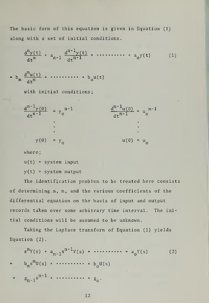
The basic form of this equation is given in Equation (1)
along with a set of initial conditions
.
§*XlH a .
dn'V(t) + + a y(t) (1)dt
n n_1dt
n_1 °
= b dVtl + + b um j . m oat
(t)
with initial conditions
;
d^yCO) - yn-l d
m " 1u(0) _ m-1
dtn-l >o
dtm-l o
y(0) = you(0) = u
q
where
;
u(t) = system input
y(t) = system output
The identification problem to be treated here consists
of determining n, m, and the various coefficients of the
differential equation on the basis of input and output
records taken over some arbitrary time interval. The ini-
tial conditions will be assumed to be unknown.
Taking the Laplace transform of Equation (1) yields
Equation (2)
.
snY(s) + a
n _ 1sn_1
Y(s) * + aoY(s) (2)
bm smU(s) + + b
QU(s)
n-ln-l*' B o
+g.-i s + + g
12


The g- coefficients account for the contributions of the
initial conditions. Dividing Equation (2) by s is
equivalent to integrating n+1 times in the time domain.
mi a . H*l + a m.n-1 * o n+1s s s
(3)
= b —nisi * b -m>m n-m+1 o n+1s s
+ Vi — + 6 o n+1s
Taking the inverse transform of Equation (3) results in
Equation (4)
.
tk
tk £k
Jy(t)dt + a
n _ 1 J Jy(t)dt 2 +
h+ a
o
n+l«" I y(t)dt
o
n+1
(4)
= bm
o
n-m+1 • -
•
r *.\ j*n-m+lu(t)dt + •
+ gn-1
+ b
\k *k
n+l»«- / u(t)dt
o
n+1
Sk *k
dt 2 + • • • + gn+1
• «n+l» •
oo ooSince the system is time invariant nothing has been lost by
setting the lower limit on the integrals equal to zero.
13

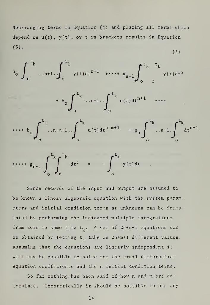
Rearranging terms in Equation (4) and placing all terms which
depend on u(t) , y(t) , or t in brackets results in Equation
(5).(5)
rtk
rtk
j^k *kL
o / ..n+1../ y(t)dtn+1 +•-•+ an _ 1 / y(t
*^ o o
r^k r^k+ b
Q/ . .n+1. . / u(t)dtn+1 + •-•
)dt
+ bm
rtk f *k r
tk r\
I ..n-m+1../ u(t)dtn" m+1
+ g Q/ ..n + l.J dt
n+1
+ "' + g n-lJ J
dt 2= - / y(t)dt
o *o o
Since records of the input and output are assumed to
be known a linear algebraic equation with the system param-
eters and initial condition terms as unknowns can be formu-
lated by performing the indicated multiple integrations
from zero to some time t-, . A set of 2n+m+l equations can
be obtained by letting t, take on 2n+m+l different values.
Assuming that the equations are linearly independent it
will now be possible to solve for the n+m+1 differential
equation coefficients and the n initial condition terms.
So far nothing has been said of how n and m are de-
termined. Theoretically it should be possible to use any
14


n' and m' greater than the actual order of the system under
study. If the order of the system is n with m input coef-
ficients then one would expect the following:
a. = for ( < i < n'-n-l )
b. = for ( < i < m'-m-l )
with n'>n and m'>m.
The model should essentially reduce itself to the right order
by setting nonessential terms equal to zero.
Unfortunately the situation is not quite this simple.
Due to the finite accuracy of all experimental data the lin-
ear equations will not have an exact solution. For certain
types of inputs the linear equations will not even be lin-
early independent. These problems can be overcome to some
extent by formulating more than 2n+m+l equations which are
required. The overdetermined set can then be solved using
the method of least squares. If the limited accuracy of
the experimental data can be attributed to round off errors
then integrating the data over a time interval much greater
than the sampling interval should remove much of the uncer-
tainty in the linear equation coefficients. This is be-
cause the roundoff process can be modeled as a zero mean
white noise process. The integral of the noise will ap-
proach zero as the period of integration increases.
Even the measures mentioned above will not solve the
problem completely however. Due to the finite precision
used to represent numbers in a computer and the iterative
15

nature of the numerical methods used to solve overdeter-
mined sets of linear equations it is impossible to obtain
zero as a solution for any parameter. If the parameter
should be zero the numerical method will return a very
small but nonzero value. Although this will result in an
incorrect estimate of the system order the error will not
be serious in most cases. This is because the small co-
efficients of the terms which should nonexistent will make
their effect negligible. Examples in Chapter III will
demonstrate this point.
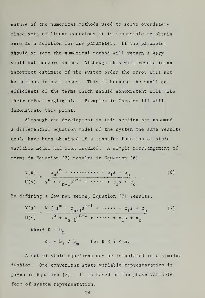
Although the development in this section has assumed
a differential equation model of the system the same results
could have been obtained if a transfer function or state
terms in Equation (2) results in Equation (6)
.
Y(s) b sm
+ + b-.s + b (6)_ _ m 1 o—i ill,..
B
U(s) s + a ,s + + a n s + av * n-1 1 o
By defining a few new terms, Equation (7) results.
Y(s) K ( sm
+ c tS1 " 1
+ + c,s + c (7)v J
\m- 1 1 o v *
ii r \ n n-1U(s) s + a ,s + + a, s + a
n-1 1 o
where K = bm
c. = b. / b for < i < m.i i m - -
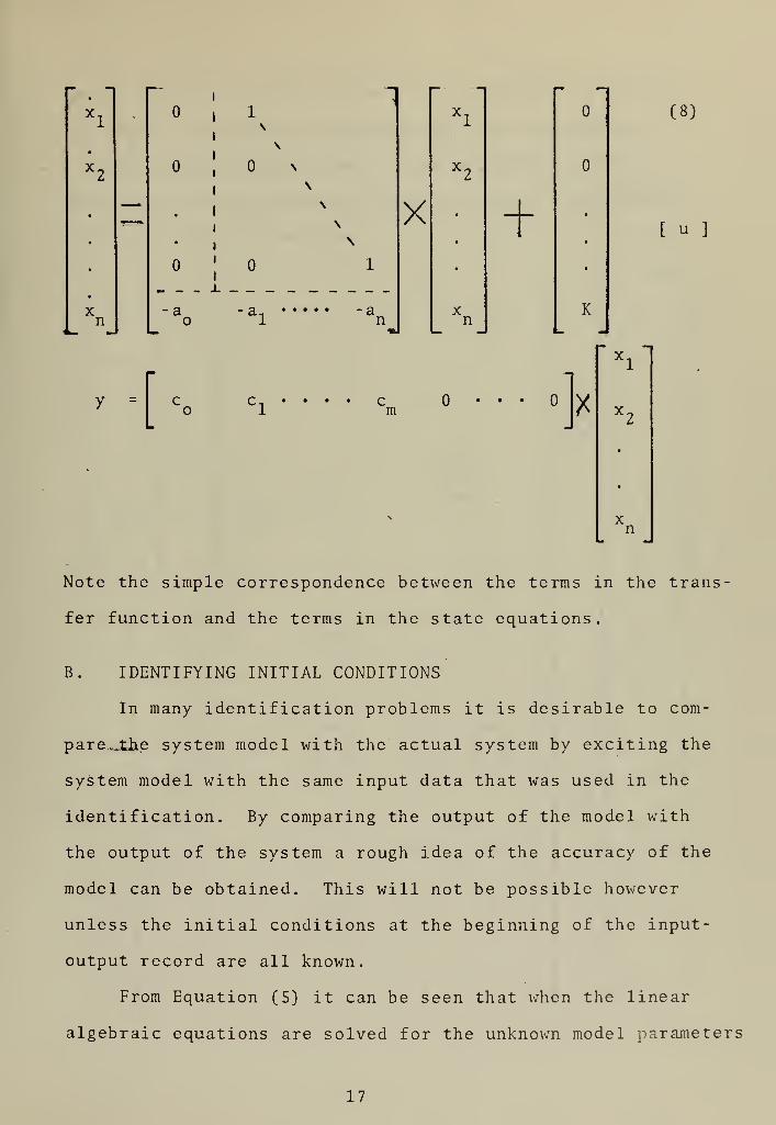
A set of state equations may be formulated in a similar
fashion. One convenient state variable representation is
given in Equation (8) . It is based on the phase variable
form of system representation.
16

L<1
h
1\
\
N
-an
xl
X2
X•+
•
.
Xn
*
K_ a
(8)
[ u ]
• • cm
n
Note the simple correspondence between the terms in the trans-
fer function and the terms in the state equations.
B. IDENTIFYING INITIAL CONDITIONS
In many identification problems it is desirable to com-
pare»..the system model with the actual system by exciting the
system model with the same input data that was used in the
identification. By comparing the output of the model with
the output of the system a rough idea of the accuracy of the
model can be obtained. This will not be possible however
unless the initial conditions at the beginning of the input-
output record are all known.
From Equation (5) it can be seen that when the linear
algebraic equations are solved for the unknown model parameters
17


the g- initial condition terms are also found. By taking
the Laplace Transform of Equation (1) and specifically-
writing in the contributions of the individual initial
conditions a relationship between the g. terms and the ini
tial conditions can be found.
(9)
^o
8l
gn-2
gn-l
al
a2
a2
a3
a . 1n-1
/
//
/a , 1n-1
X
y.
y,
y<n-2
o
n-1
X
C-. C n • • • C 1 112 m-
1
c2
C3 '
//
/ '
'm-1 1
. .
. .
. .
X
u
u
u
11
m-2
m-1
18


Unfortunately Equation (9) requires the knowledge of
m-1 derivatives of the input function u. It may be neces-
sary to calculate m-1 derivatives of the input using numer-
ical techniques. This could cause the model and system
output to differ slightly at the beginning of the output
record but as the natural response dies out the records
should converge. It may be possible to avoid this diffi-
culty in many cases by choosing the beginning of the input-
output record at a point where the input is relatively
constant
.
C. SIMPLIFICATIONS WITH ZERO INITIAL CONDITIONS
In many problems it will be possible to exercise com-
plete control over the input to the system under study. If
it is possible to obtain an input-output record beginning
when the system is in the zero state it will be possible to
simplify the identification procedure. Since the g. terms
will all be zero if the system is in the zero state they
need not be included in the formulation of the linear alge-
braic equations. This will reduce the number of unkno\^ns
from 2n+m+l to n+m+1.
It should be noted that additional information can
often be incorporated into the identification procedure in
order to simplify the problem. For example if the steady
state gain constant were known the number of unknowns could
be reduced by one. It is usually a simple matter to tell
whether a system has poles or zeroes at the origin. This
19


piece of information can easily be used to simplify the
identification procedure still further. As a general rule,
the fewer the unknowns the more accurate the identification.
20


III. IMPLEMENTATION
A. NUMERICAL METHODS
The identification technique presented in Chapter II
can be broken into two basic steps. The first step con-
sists of performing the multiple integrations of the input
and output and forming the overdetermined set of linear
algebraic equations. The second step consists of solving
the linear equations for the unknown model parameters. It
is a distinct advantage of the identification technique
under study that each of these steps can be carried out by
subprograms that are readily available in virtually all
modern computer centers.
Step one can be handled by any numerical integration
subroutine. Although there are quite a few highly sophis-
ticated numerical integration procedures available, trape-
zoidal integration will give better results in most
applications. There are several reasons why this is true.
First of all, most of the more complex integration tech-
niques perform poorly when the function being integrated
is discontinuous. Since control system inputs are often
discontinuous and since such discontinuities are quite
desirable from an identification standpoint, complex inte-
gration techniques are usually undesirable. Even when the
functions to be integrated are continuous the slight im-
provement in accuracy offered by more advanced methods is
not enough to justify the tremendous increase in computation-
al load associated with their use.
21

Step two, the solution of the set of overdete mined
linear equations, is a classical problem in several fields
of mathematics and engineering. Unfortunately most of the
classical techniques for solving such problems are not
practical. They tend to magnify the errors introduced by
the finite precision of the computer to the point where
the solution is meaningless. Fortunately several modern
methods are available that display more acceptable behavior
The method used in this paper was developed by Golub [31]
in 1965. The basic approach is to triangularize the coef-
ficient matrix by performing a Choleski decomposition. The
decomposition is accomplished by applying repeated House-
holder transformations [32] . Once the coefficient matrix
has been triangularized the unknowns can be obtained by
back substitution. The method is quite stable numerically
and is capable of handling illconditioned coefficient ma-
trices .
B. CHARACTERISTICS OF GOOD INPUT-OUTPUT RECORDS
The accuracy with which a system can be identified is
strongly dependent on the input-output record used in the
identification. Since parameters are identified on the
basis of their effect on the output it will be impossible
to identify a parameter unless its effect is measureable.
If the input to a system has a frequency spectrum that is
more or less uniform over the frequency range of interest
the identification will probably be very good. If the
22

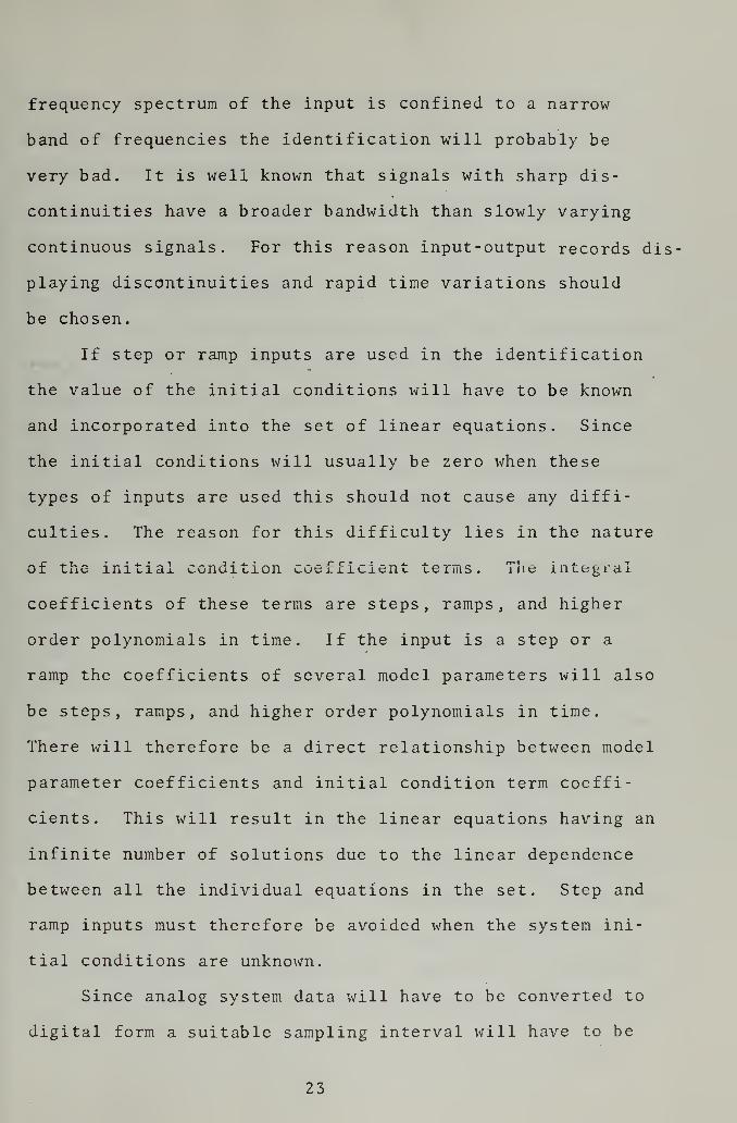
frequency spectrum of the input is confined to a narrow
band of frequencies the identification will probably be
very bad. It is well known that signals with sharp dis-
continuities have a broader bandwidth than slowly varying
continuous signals. For this reason input-output records dis
playing discontinuities and rapid time variations should
be chosen.
If step or ramp inputs are used in the identification
the value of the initial conditions will have to be known
and incorporated into the set of linear equations. Since
the initial conditions will usually be zero when these
types of inputs are used this should not cause any diffi-
culties. The reason for this difficulty lies in the nature
of the initial condition coefficient terms. The integral
coefficients of these terms are steps, ramps, and higher
order polynomials in time. If the input is a step or a
ramp the coefficients of several model parameters will also
be steps, ramps, and higher order polynomials in time.
There will therefore be a direct relationship between model
parameter coefficients and initial condition term coeffi-
cients. This will result in the linear equations having an
infinite number of solutions due to the linear dependence
between all the individual equations in the set. Step and
ramp inputs must therefore be avoided when the system ini-
tial conditions are unknown.
Since analog system data will have to be converted to
digital form a suitable sampling interval will have to be
23


chosen. Experimental results have shown that a sampling
rate ten to one hundred times shorter than the shortest
system time constant works quite well. Lower sampling
rates may introduce inaccuracies in the location of high
frequency poles and zeroes.
C. PROGRAM DESCRIPTION
In order to evaluate experimentally the characteristics
of the identification procedure under study a set of digital
computer programs was developed. The main identification
program is a direct implementation of the procedure develop-
ed in Chapter II. Subroutine SYSTEM is a simulation program
that was written to generate input-output data for the main
program to process.
In the beginning of the identification program several
important parameters are defined. NP and NZ are rough es-
timates of the number of poles and the number of zeroes in
the system to be identified. KPTMAX is the number of sam-
ple points available in the input-output record. Each sam-
ple point will consist of the time (T) , the input amplitude
(R) , and the output amplitude (C) . IPTS is the number of
sample points that will separate successive linear equa-
tions. In other words, every time the total number of points
read in is a multiple of IPTS a linear equation will be gen-
erated. The total number of linear equations that will be
generated is equal to KPTMAX/ IPTS. When all of the linear
equations have been formed subroutine DLLSQ is called. This
24

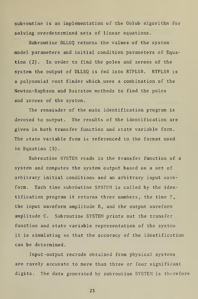
subroutine is an implementation of the Golub algorithm for
solving overdetermined sets of linear equations.
Subroutine DLLSQ returns the values of the system
model parameters and initial condition parameters of Equa-
tion (2) . In order to find the poles and zeroes of the
system the output of DLLSQ is fed into RTPLSB. RTPLSB is
a polynomial root finder which uses a combination of the
Newton-Raphson and Bairstow methods to find the poles
and zeroes of the system.
The remainder of the main identification program is
devoted to output. The results of the identification are
given in both transfer function and state variable form.
The state variable form is referenced to the format used
in Equation (8)
.
Subroutine SYSTEM reads in the transfer function of a
system and computes the system output based on a set of
arbitrary initial conditions and an arbitrary input wave-
form. Each time subroutine SYSTEM is called by the iden-
tification program it returns three numbers, the time T,
the input waveform amplitude R, and the output waveform
amplitude C. Subroutine SYSTEM prints out the transfer
function and state variable representation of the system
it is simulating so that the accuracy of the identification
can be determined.
Input-output recrods obtained from physical systems
are rarely accurate to more than three or four significant
digits. The data generated by subroutine SYSTEM is therefore
25


rounded off by subroutine ROUND before being passed to the
identification program. The number of significant digits
in the data returned to the identification program may be
varied by changing the value of the parameter NA in the
simulation subroutine.
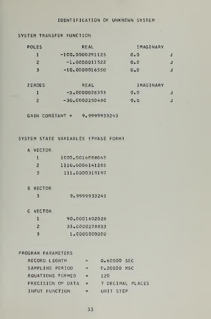
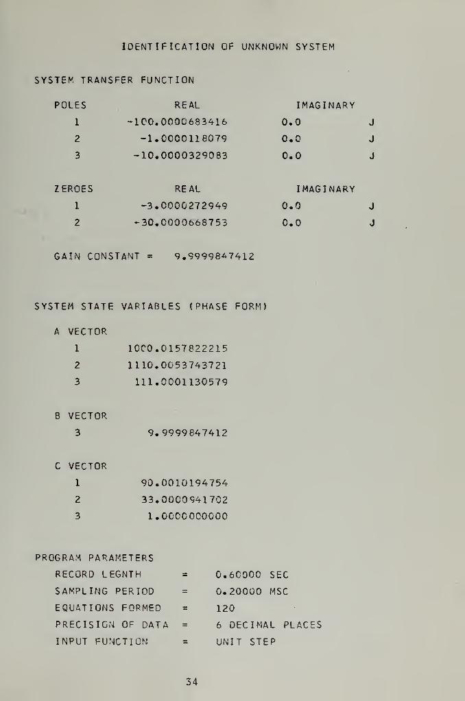
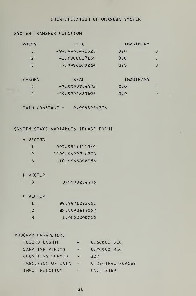
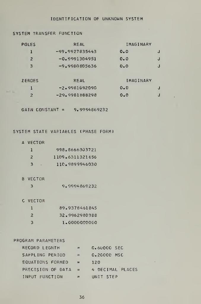
D. EXAMPLES
The following examples demonstrate how the accuracy of
an identification depends on the accuracy of the input-
output record, the sampling period, and the input waveform.
They also show how the order of the system can be deter-
mined from a trial identification run using an estimated
order greater than the actual order of the system.
Example one illustrates the relationship between the
accuracy of the input-output record data and the resulting
identification. In order to minimize the effect of other
factors all initial conditions were set equal to zero, a
step input was used, and n' and m' were set equal to n and
m. Example one demonstrates the fact that there is a di-
rect (almost linear) relationship between the accuracy of
input-output data and the accuracy of the identification.
Note that even when the input-output record contained only
two significant digits the identification of the system
poles and zeroes was within about three percent of their
exact values
.
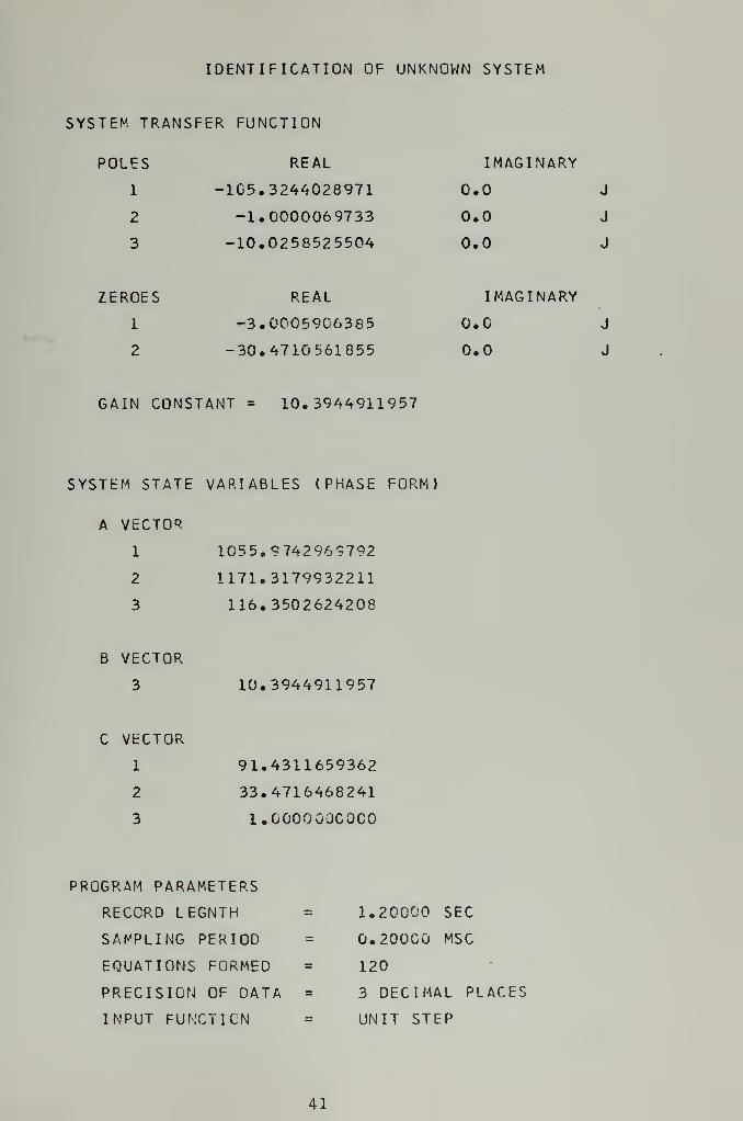
Example two illustrates the relationship between the
sampling period used with the input-output records and the
26

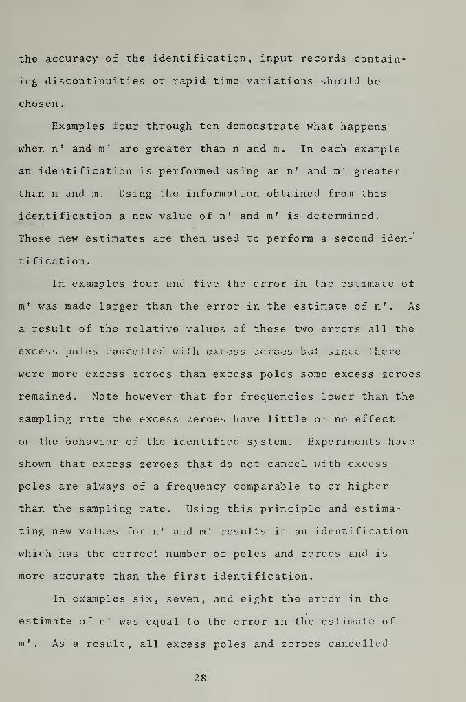
the accuracy of the identification, input records contain-
ing discontinuities or rapid time variations should be
chosen.
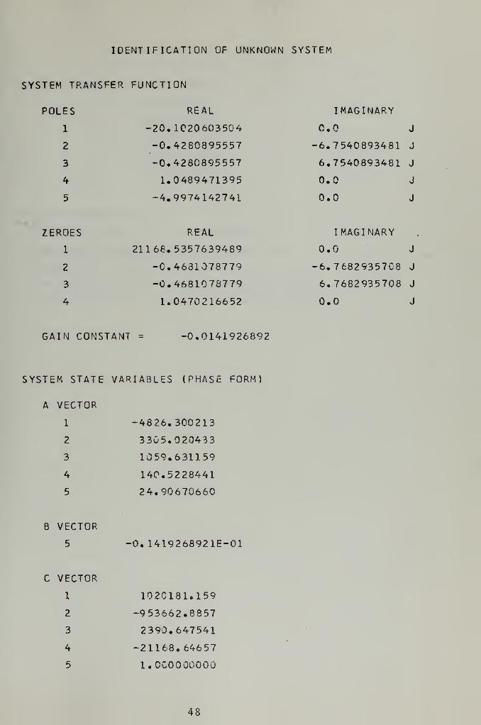
Examples four through ten demonstrate what happens
when n' and m' are greater than n and m. In each example
an identification is performed using an n' and m' greater
than n and m. Using the information obtained from this
identification a new value of n' and m' is determined.
These new estimates are then used to perform a second iden-
tification.
In examples four and five the error in the estimate of
m' was made larger than the error in the estimate of n'. As
a result of the relative values of these two errors all the
excess poles csnccuSu with excess zeroes but since tucre
were more excess zeroes than excess poles some excess zeroes
remained. Note however that for frequencies lower than the
sampling rate the excess zeroes have little or no effect
on the behavior of the identified system. Experiments have
shown that excess zeroes that do not cancel with excess
poles are always of a frequency comparable to or higher
than the sampling rate. Using this principle and estima-
ting new values for n' and m* results in an identification
which has the correct number of poles and zeroes and is
more accurate than the first identification.
In examples six, seven, and eight the error in the
estimate of n' was equal to the error in the estimate of
m'. As a result, all excess poles and zeroes cancelled
28


with each other leaving a system of the correct order.
Note that by repeating the identification with the correct
value of n' and m' it was possible to improve the accuracy
of the identification.
In examples nine and ten the error in the estimate
of n' was made greater than the error in the estimate of
m'. As a result, all excess zeroes cancelled with excess
poles but some excess poles remained. Note that for fre-
quencies lower than the sampling rate the excess poles
have negligible effect. Experiments have shown that excess
poles that do not cancel with excess zeroes are almost al-
ways of a frequency comparable to or greater than the sam-
pling rate. Using this principle and estimating new values
for n ' and m 1 resulted in a correct identification of the
simulated systems.
Experiments have shown that identifications involving
uncancelled excess zeroes are generally more accurate than
identifications involving uncancelled excess poles. For
this reason it is best to set m' close to n' when identi-
fying an unknown system.
Using the experimental findings described above a
simple procedure for determining n and m can be formulated.
First, guess an n' which is greater than the order of the
system to be identified. This should not be too difficult
in most engineering identification problems. Let m' be
equal to n' or m'-l. This will guarantee complete cancel-
lation of all excess poles and zeroes or partial cancellation
29


of excess poles and zeroes with excess zeroes remaining.
After making a trial identification with the values of n'
and m' mentioned above, estimate new values for n' and m'
based on the reasoning in the examples. The new values
of n' and m' should now be correct. By performing the
identification with these values of n' and m' a good iden-
tification should result.
30


EXAMPLE 1.
SYSTEM TO BE IDENTIFIED
SYSTEM TRANSFER FUNCTION
POLES REAL
1 -1,0000000000
2 -10.0000000000
3 -100.C000000000
ZEROES REAL
1 -3.0003000000
2 -30.0000COOOCO
GAIN CONSTANT = 10.0000000000
SYSTEM STATE VARIABLES (PHASE FORM)
A VECTOR
1 ICOO.OGOOOOOOOO
2 111C.C0000000C0
3 lll.OCOOOOOOOO
B VECTOR
3 10.0000000000
C VECTOR
1 90.0000000000
2 33.C0000000C0
3 l.COOOCOOOCD
IMAGINARY
0.0 J
0.0 J
0.0 J
IMAGINARY
0.0 J
0.0 J
31

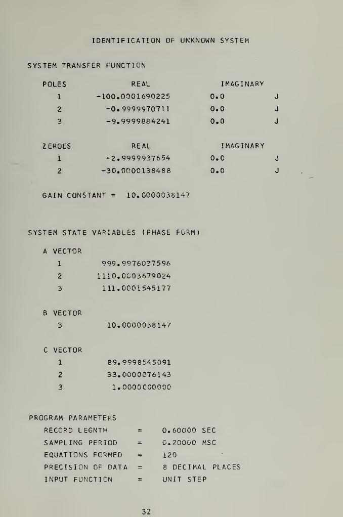
IDENTIFICATION OF UNKNOWN SYSTEM
SYSTEM TRANSFER FUNCTION
POLES REAL I MAGilNARY
1 -100.0001690225 0.0 J
2 -0.9999970711 0.0 J
3 -9.9999884241 0.0 J
ZEROES REAL IMAGINARY
1 -2.9999937654 0.0 J
2 -30.0000138488 0.0 J
GAIN CONSTANT = 10. CC00038147
SYSTEM STATE VARIABLES (PHASE FORM)
A VECTOR
1 999.9976037596
2 1110.CC03679024
3 111.0001545177
B VECTOR
3 10.0000038147
C VECTOR
1 89.9998545091
2 33.0000076143
3 1.0000000000
PROGRAM PARAMETERS
RECORD LEGNTH
SAMPLING PERIOD
EQUATIONS FORMED
PRECISION OF DATA
INPUT FUNCTION
0.60000 SEC
0.20000 MSC
120
8 DECIMAL PLACES
UNIT STEP
32

IDENTIFICATION OF UNKNOWN SYSTEM
SYSTEM TRANSFER FUNCTION
POLES REAL IMAGINARY
1 -ICO. 0000291125 0.0 J
2 -1.0000011522 0.0 J
3 -10.0000016550 0.0 J
ZEROES REAL IMAGINARY
1 -3.0000028353 0.0 J
2 -30.0000250480 0.0 J
GAIN CONSTANT = 9.9999933243
SYSTEM STATE VARIABLES (PHASE FORM)
A VECTOR
1 1C00.0016C88045
2 1110.0006141285
3 111.0000319197
B VECTOR
3 9.9999933243
C VECTOR
1 90.0001602028
2 33.0000278833
3 l.COOGOCOCOO
PROGRAM PARAMETERS
RECORD LEGNTH = 0.60000 SEC
SAMPLING PERIOD = C. 20000 MSC
EQUATIONS FORMED = 120
PRECISION OF DATA = 7 DECIMAL PLACES
INPUT FUNCTION = UNIT STEP
33

IDENTIFICATION OF UNKNOWN SYSTEM
SYSTEM TRANSFER FUNCTION
POLES
1
2
3
REAL
-100.000C683416
-1.0000118079
-10.0000329083
IMAGINARY
0.0 J
0.0 J
0.0 J
ZEROES
1
2
REAL
-3.0000272949
-30.0000668753
IMAGINARY
0.0 J
0.0 J
GAIN CONSTANT = 9.99998*7412
SYSTEM STATE VAPIABLES (PHASE FORM)
A VECTOR
1 10C0. 0157822215
2 1110.0053743721
3 111.0001130579
B VECTOR
3 9.9999 847412
C VECTOR
1 90.0010194754
2 33.0000941702
3 l.OOCCOCOOOO
PROGRAM PARAMETERS
RECORO LEGNTH
SAMPLING PERIOD
EQUATIONS FORMED
PRECISION OF DATA
INPUT FUNCTION
0.60000 SEC
0.20000 MSC
120
6 DECIMAL PLACES
UNIT STEP
34

IDENTIFICATION OF UNKNOWN SYSTEM
SYSTEM TRANSFER FUNCTION
POLES REAL IMAGINARY
1 -99.9968491528 0.0 J
2 -1.CG00017165 0.0 J
3 -9.9998390264 0.0 J
ZEROES REAL IMAGINARY
1 -2.9999754422 0.0 J
2 -29.9992863605 0.0 J
GAIN CONSTANT = 9.9998254776
SYSTEM STATE VARIABLES (PHASE FORM)
A VECTOR
1 999.9541111369
2 1109.9492716708
3 110.9966898958
B VECTOR
3 9.9998254776
C VECTOR
1 89.9971223661
2 32.9992618027
3 1,0000 000000
PROGRAM PARAMETERS
RECORD LEGNTH = 0.60000 SEC
SAMPLING PERIOD = 0.20000 MSC
EQUATIONS FORMED = 120
PRECISION OF DATA = 5 DECIMAL PLACES
INPUT FUNCTION = UNIT STEP
35

IDENTIFICATION OF UNKNOWN SYSTEM
SYSTEM TRANSFER FUNCTION
POLES REAL IMAGINARY
1 -99.9927835443 0.0 J
2 -0.9991304951 0.0 J
3 -9.9980805636 0.0 J
ZEROES REAL IMAGINARY
1 -2.9981092090 0.0 J
2 -29.9981888298 0.0 J
GAIN CONSTANT = 9.99 94869232
SYSTEM STATE VARIABLES (PHASE FORM)
A VECTOR
1 998.8666303721
2 1109.6311321656
3 11C. 9899946030
B VECTOR
3 9.9994869232
C VECTOR
1 89.9378461845
2 32.9962980388
3 1.0000000000
PROGRAM PARAMETERS
RECORD LEGNTH
SAMPLING PERIOD
EQUATIONS FORMED
PRECISION OF DATA
INPUT FUNCTION
C.6U00C SEC
0.20000 MSC
120
4 DECIMAL PLACES
UNIT STEP
36

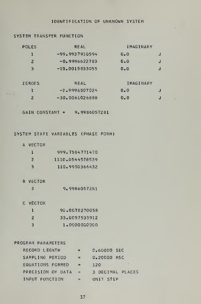
IDENTIFICATION OF UNKNOWN SYSTEM
SYSTEM TRANSFER FUNCTION
POLES
1
2
3
REAL
-99.9937910594
-0.9996622783
-10.0015833055
IMAGINARY
0.0 J
0.0 J
0.0 J
ZEROFS
1
2
REAL
-2.9996507024
-30.0061026888
IMAGINARY
0.0 J
0.0 J
GAIN CONSTANT = 9.9986057281
SYSTEM STATE VARIABLES (PHASE FORM)
A VECTOR
1 999.7584771470
2 1110.0544578539
3 110.9950366432
B VECTOR
3 9.9986057281
C VECTOR
1 90.0078270058
2 33.0057533912
3 1 .0000 000000
PROGRAM PARAMETERS
RECORD LEGNTH
SAMPLING PERIOD
EQUATIONS FORMED
PRECISION OF DATA
INPUT FUNCTION
0.60000 SEC
0.20000 MSC
120
3 DECIMAL PLACES
UNIT STEP
37


IDENTIFICATION OF UNKNOWN SYSTEM
SYSTEM TRANSFER FUNCTION
POLES REAL IMAGINARY
1 -98.8004578528 0.0 J
2 -0.9763637189 0.0 J
3 -9.8862584052 0.0 J
ZEROES REAL IMAGINARY
1 -2.9406610975 0.0 J
2 -29.6497245014 0.0 J
GAIN CONSTANT = 9.9451894760
SYSTEM STATE VARIABLES (PHASE FORM)
A VECTOR
1 953.6797208413
2 1082.8846233636
3 109. 6630799769
B VECTOR
3 9.9451894760
C VECTOR
1 87.1897913926
2 32. 5903855989
3 1.0000000000
PROGRAM PARAMETERS
RECORD LEGNTH = 0.60000 SEC
SAMPLING PERIOD = 0.20000 MSC
EQUATIONS FORMED = 120
PRECISION OF DATA = 2 DECIMAL PLACES
INPUT FUNCTION = UNIT STEP
38

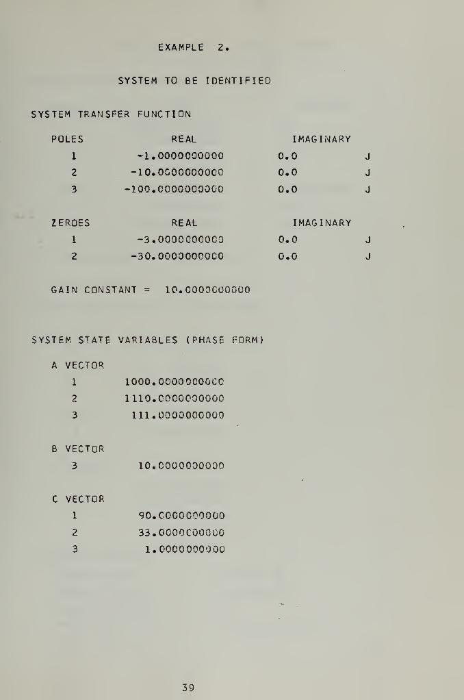
EXAMPLE 2.
SYSTEM TO BE IDENTIFIED
SYSTEM TRANSFER FUNCTION
POLES REAL IMAGINARY
1 -1,0000000000 0.0 J
2 -10,0000000000 0.0 J
3 -100.0000000000 0.0 J
ZEROES REAL IMAGINARY
1 -3. OOOOCOOOOO 0.0 J
2 -30.0000000000 0.0 J
GAIN CONSTANT = 10. OOOOCOOOOO
SYSTEM STATE VARIABLES (PHASE FORM)
A VECTOR
1 1000.0000000000
2 1110.C00000000C
3 111.0000000000
B VECTOR
3 10.0000000000
C VECTOR
1 90.COCOCOOOOO
2 33. OOOOCOOOOO
3 1.0000000000
39


IDENTIFICATION OF UNKNOWN SYSTEM
SYSTEM TRANSFER FUNCTION
POLES REAL IMAGINARY
1 -101.0610717819 0.0 J
2 -1.0000331312 0.0 J
3 -10.0017011716 0.0 J
ZEROES REAL IMAGINARY
1 -3.0002183624 0.0 J
2 -30.0553440030 0.0 J
GAIN CONSTANT = 10.0887174606
SYSTEM STATE VARIABLES (PHASE FORM)
A VECTOR
1 1010.8161234948
2 1121.8490926385
3 112.0628060847
B VECTOR
3 10.0887174606
C VECTOR
1 90.1725949663
2 33.0555623654
3 1.0000000000
PROGRAM PARAMETERS
RECORD LE(SNTH = 0.6COOO SEC
SAMPLING !PERIOD = 0.10000 MSC
EQUATIONS FORMED = 120
PRECISION QP DATA = 3 DECIMAL PLACES
INPUT FUNCTION UNIT STEP
40

IDENTIFICATION OF UNKNOWN SYSTEM
SYSTEM. TRANSFER FUNCTION
POLES REAL IMAGINARY
1 -1G5. 3244028971 0.0 J
2 -1.000006 9733 0.0 J
3 -10.0258525504 0.0 J
ZEROES REAL IMAGINARY
1 -3.0005906385 0.0 J
2 -30.4710561855 0.0 J
GAIN CONSTANT = 10.3944911957
SYSTEM STATE VARIABLES (PHASE FORM)
A VECTOR
1 1055.9742969792
2 1171.3179932211
3 116.3502624208
B VECTOR
3 10.3944911957
C VECTOR
1 91.4311659362
2 33.4716468241
3 l.GOOOGOCOCO
PROGRAM PARAMETERS
RECORD LEGNTH = 1.20000 SEC
SAMPLING PERIOD 0.200C0 MSC
EQUATIONS FORMED = 120
PRECISION OF DATA 3 DECIMAL PLACES
INPUT FUNCTION = UNIT STEP
41


IDENTIFICATION OF UNKNOWN SYSTEM
SYSTEM TRANSFER FUNCTION
POLES REAL IMAGINARY
1 -107.6394221979 0.0 J
2 -1.0000162038 0.0 J
3 -10.0077785631 0.0 J
ZEROES REAL IMAGINARY
1 -3.0001692900 0.0 J
2 -30.3047449110 0.0 J
GAIN CONSTANT = 10.6635513306
SYSTEM STATE VARIABLES (PHASE FORM)
A VECTOR
1 1C77. 2489572831
2 1194.8806091150
3 118.6472169649
B VECTOR
3 10.6635513306
C VECTOR
1 90. 9193650217
2 33.3C49142C09
3 1.0000000000
PROGRAM PARAMETERS
RECORD LEGNTH = 3.00000 SEC
SAMPLING PERIOD = 0.50000 MSC
EQUATIONS FORMED = 120
PRECISION OF DATA = 3 DECIMAL PLACES
INPUT FUNCTION = UNIT STEP
42

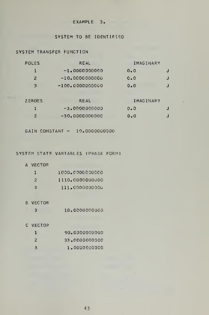
EXAMPLE 3.
SYSTEM TO BE IDENTIFIED
SYSTEM TRANSFER FUNCTION
POLES REAL
1 -1.0000000000
2 -10.0000000000
3 -100.0000000000
ZEROES REAL
1 -3.0000000000
2 -30.0000000000
IMAGINARY
0.0 J
0.0 J
0.0 J
IMAGINARY
0.0 J
0.0 J
GAIN CONSTANT = 10.0000000000
SYSTEM STATE VARIABLES (PHASE FORM)
A VECTOR
1 1000.COOCOOOOCO
2 1110.0000000000
3 111.0000000000
B VECTOR
3 10.0000000000
C VECTOR
1 90.0000000000
2 33.OCO0O0O000
3 l.OOOOOOOOCO
43

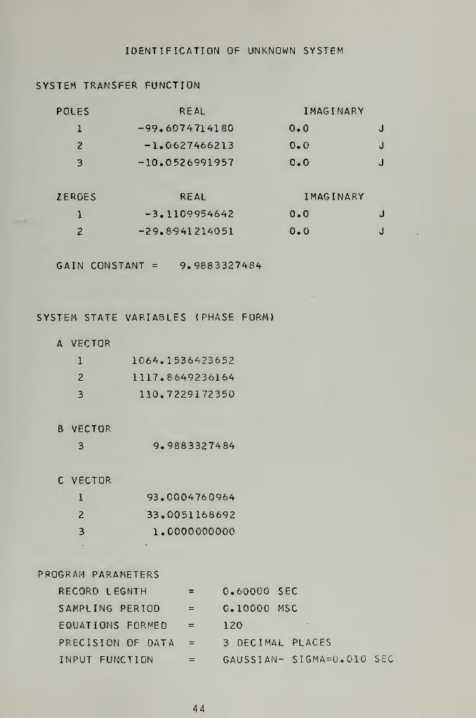
IDENTIFICATION OF UNKNOWN SYSTEM
SYSTEM TRANSFER FUNCTION
POLES
1
2
3
REAL
-99.6074714180
-1.0627466213
-10.0526991957
IMAGINARY
0.0 J
0.0 J
0.0 J
ZEROES
1
2
REAL
-3.1109954642
-29.8941214051
IMAGINARY
0.0 J
0.0 J
GAIN CONSTANT = 9.9883327484
SYSTEM STATE VARIABLES (PHASE FORM)
A VECTOR
1 1C64. 1536423652
2 1117.8649236164
3 110.7229172350
B VECTOR
3 9.9883327484
C VECTOR
1 93.0004760964
2 33.0051168692
3 1.0000000000
PROGRAM PARAMETERS
RECORD LEGNTH
SAMPLING PERIOD
EQUATIONS FORCED
PRECISION OF DATA
INPUT FUNCTION
0.60000 SEC
C. 10000 MSC
120
3 DECIMAL PLACES
GAUSSIAN- SIGMA=U.010 SEC
44

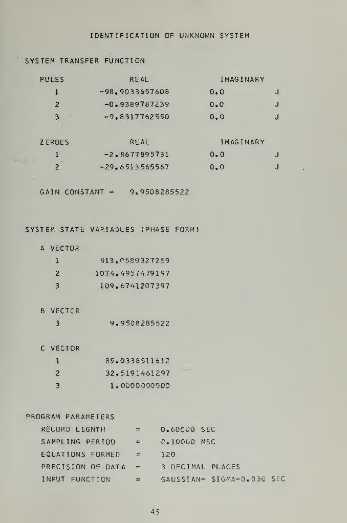
IDENTIFICATION OF UNKNOWN SYSTEM
SYSTEM TRANSFER FUNCTION
POLES REAL
1 -98.9033657608
2 -0.9389787239
3 -9.8317762550
ZEROES REAL
1 -2.8677895731
2 -29.6513565567
IMAGINARY
0.0 J
0.0 J
0.0 J
IMAGINARY
0.0 J
0.0 J
GAIN CONSTANT = 9.9508285522
SYSTEM STATE VARIABLES (PHASE FORM)
A VECTOR
1 913.0589327259
2 1074.4957479197
3 109.6741207397
B VECTOR
3 9.9508285522
C VECTOR
1 85.0338511612
2 32.5191461297
3 1.0000000000
PROGRAM PARAMETERS
RECORD LEGNTH
SAMPLING PERIOD
EQUATIONS FORMED
PRECISION OF DATA
INPUT FUNCTION
0.60COO SEC
C. 10000 MSC
120
3 DECIMAL PLACES
GAUSSIAN- SIGMA=0.030 SEC
45


IDENTIFICATION OF UNKNOWN SYSTEM
SYSTEM TRANSFER FUNCTION
POLES
1
2
3
REAL
-99.1859265460
-0.7535004508
-9.5204582353
IMAGINARY
0.0 J
0.0 J
0.0 J
ZEROES
1
2
REAL
-2.5186589038
-29.4122032416
IMAGINARY
CO J
0.0 J
GAIN CONSTANT = 9.9813451767
SYSTEM STATE VARIABLES (PHASE FORM)
A VECTOR
1 711.5270631979
2 1C26. 2057811417
3 109.4598852321
B VECTOR
3 9.9813451767
C VECTOR
1 74.0793075760
2 31.9308621454
3 l.OOOOOCCOGO
PROGRAM PARAMETERS
RECORD LEGNTH
SAMPLING PERIOD
EQUATIONS FORMED
PRECISION OF DATA
INPUT FUNCTION
0.6CC00 SEC
0.100C0 MSC
120
3 DECIMAL PLACES
GAUSSIAN- SIGMA=0.050 SEC
46

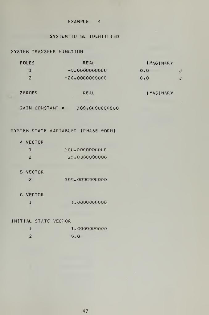
EXAMPLE 4
SYSTEM TO BE IDENTIFIED
SYSTEM TRANSFER FUNCTION
POLES
1
2
REAL
-5.0000000000
20.00C00C00C0
IMAGINARY
0,0 J
0.0 J
ZEROES REAL IMAGINARY
GAIN CONSTANT = 300.0CCOOOOOOO
SYSTEM STATE VARIABLES (PHASE FORM)
A VECTOR
1
2
100.0000000000
25.0000000000
B VECTOR
2 300.000C00C000
C VECTOR
1 l.OOOOOCOGOO
INITIAL STATE VECTOR
1 1.0000000000
2 0.0
47

IDENTIFICATION OF UNKNOWN SYSTEM
SYSTEM TRANSFER FUNCTION
POLES REAL
1 -20.1020603504
2 -0.4280895557
3 -0.4280895557
4 1.0489471395
5 -4.9974142741
ZEROES REAL
1 21168. 5357639489
2 -0.4631078779
3 -0.4681078779
4 1.0470216652
GAIN CONSTANT = -0.0141926892
SYSTEM STATE VARIABLES (PHASE FORM)
A VECTOR
1 -4826.300213
2 3305.020433
3 1059.631159
4 140,5228441
5 24.90670660
B VECTOR
5 -0. 1419268921
C VECTOR
1 102C181.159
2 -953662.8857
3 2390.647541
4 -21168. 64657
5 l.CCOOOOOOO
IMAGINARY
CO J
•6.7540893481 J
6.7540893481 J
0.0 J
0.0 J
IMAGINARY
0.0 J
6.7682935708 J
6.7682935708 J
0.0 J
48

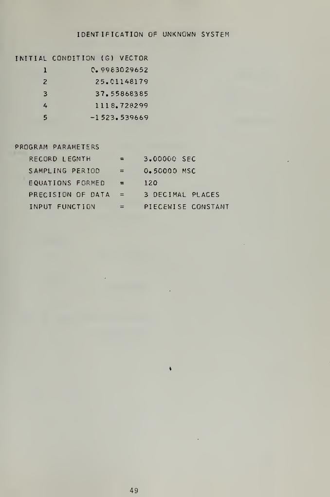
IDENTIFICATION OF UNKNOWN SYSTEM
INITIAL CONDITION (G) VECTOR
1 0.9963029652
2 25.01148179
3 37.55868385
4 1118.728299
5 -1523.539669
PROGRAM PARAMETERS
RECORD LEGNTH
SAMPLING PERIOD
EQUATIONS FORMED
PRECISION OF DATA
INPUT FUNCTION
3.00000 SEC
0.50000 MSC
120
3 DECIMAL PLACES
PIECEWISE CONSTANT
49

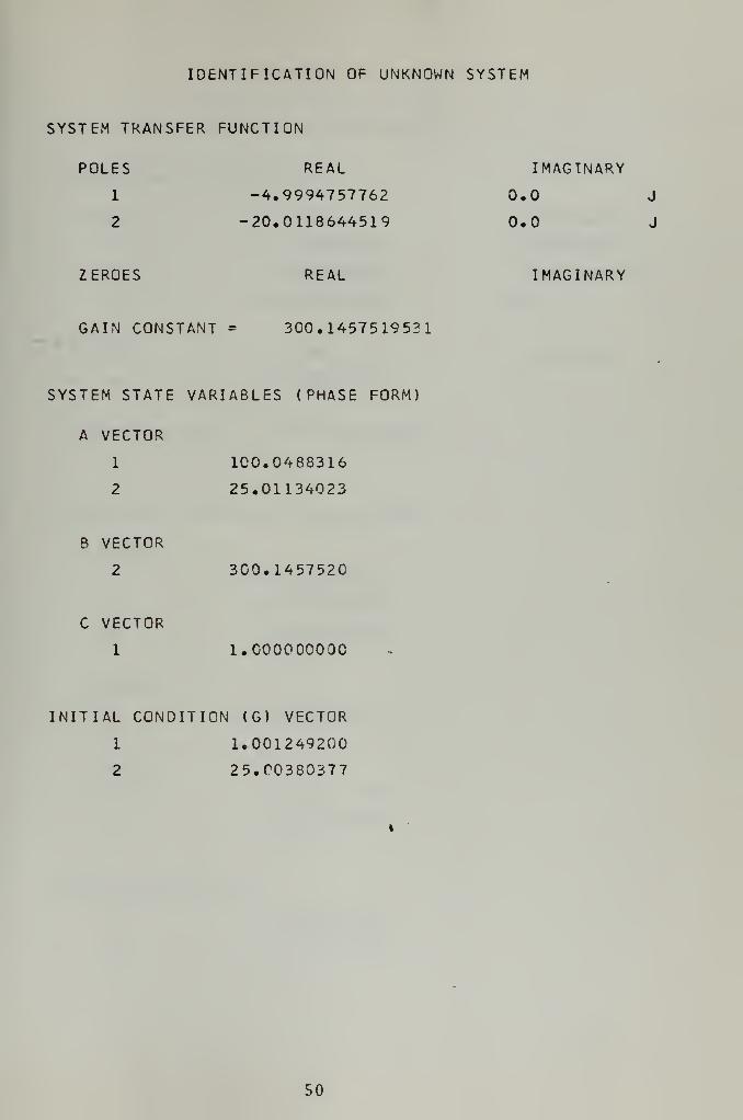
IDENTIFICATION OF UNKNOWN SYSTEM
SYSTEM TRANSFER FUNCTION
POLES REAL IMAGINARY
1 -4.9994757762 0.0 J
2 -20.0118644519 0.0 J
ZEROES REAL IMAGINARY
GAIN CONSTANT = 300.1457519531
SYSTEM STATE VARIABLES (PHASE FORM)
A VECTOR
1 100.0488316
2 25.01134023
B VECTOR
2 300.145752C
C VECTOR
1 1.000000000
INITIAL CONDITION (G) VECTOR
1 1.001249200
2 25.C0380377
50

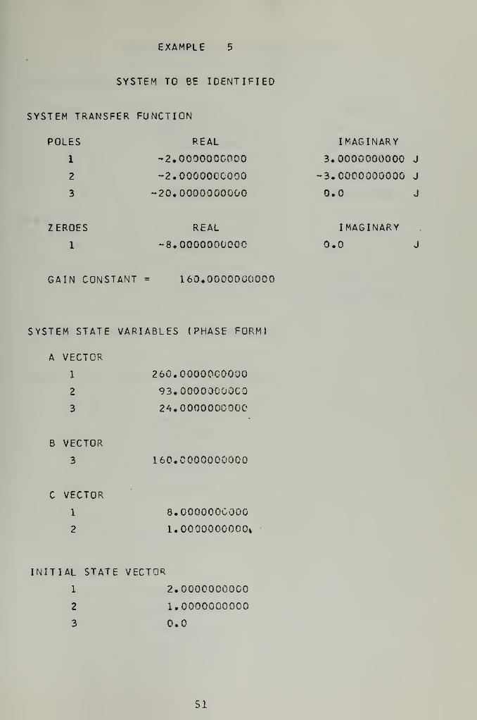
EXAMPLE
SYSTEM TO BE IDENTIFIED
SYSTEM TRANSFER FUNCTION
POLES REAL
1 -2.00000CG000
2 -2.0000000000
3 -20,0000000000
ZEROES REAL
1 -8.0000000000
IMAGINARY
3.0000000000 J
3.0000000000 J
0.0 J
IMAGINARY
0.0 J
GAIN CONSTANT = 160.0000000000
SYSTEM STATE VARIABLES (PHASE FORM)
A VECTOR
1 260.0000000000
2 93.0000000000
3 24.0000000000
B VECTOR
3 160.0000000000
C VECTOR•
1 8.0000000000
2 1.0000000000*
INITIAL STATE VECTOR
1 2.0000000000
2 1.0000000000
3 0.0
51


IDENTIFICATION OF UNKNOWN SYSTEM
SYSTEM TRANSFER FUNCTION
POLES REAL
1 -20.3839954707
2 1.0012938647
3 1.0012938647
4 -1.9998854338
5 -1.9998854338
ZEROES REAL
1 -7.6038902797
2 447.1906330529
3 1.2922226696
4 1.2922226696
GAIN CONSTANT = -0.3623618484
SYSTEM STATE VARIABLES (PHASE FORM)
A VECTOR
1 20863. 16713
2 6906.430945
3 1994.127061
4 124.3802348
5 22.38117861
B VECTOR
5 -0.3623618484
C VECTOR
1 -283455.3928
2 -27855.70425
3 -2180.940891
4 -442.1711881
5 1.000000000
IMAGINARY
0.0 J
8.8128722093 J
8.8128722093 J
3.0C17839895 J
3.0017839895 J
IMAGINARY
0.0 J
0.0 J
9.0382447685 J
9.0382447685 J
52

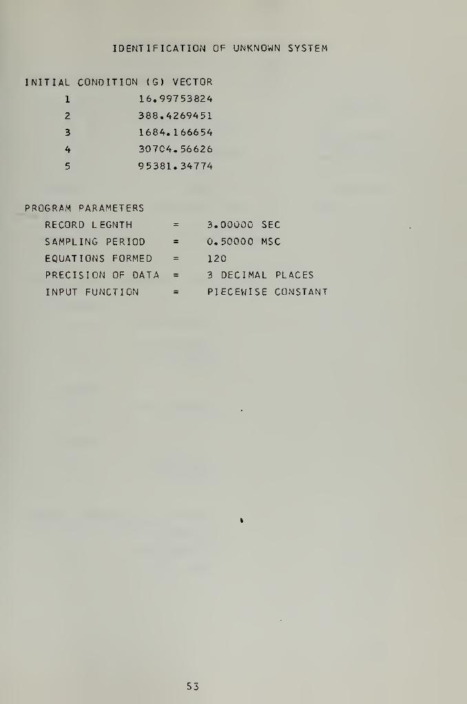
IDENTIFICATION OF UNKNOWN SYSTEM
INITIAL CONDITION (G) VECTOR
1 16,99753824
2 388.4269451
3 1684.166654
4 307C4. 56626
5 95381.34774
PROGRAM PARAMETERS
RECORD LEGNTH
SAMPLING PERIOD
EQUATIONS FORMED
PRECISION OF DATA
INPUT FUNCTION
3.00000 SEC
0.50000 MSC
120
3 DECIMAL PLACES
PIECEWISE CONSTANT
53

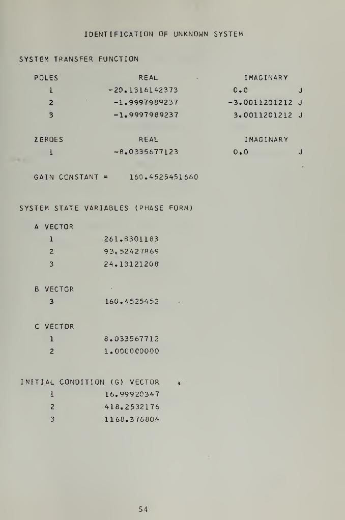
IDENTIFICATION OF UNKNOWN SYSTEM
SYSTEM TRANSFER FUNCTION
POLES REAL IMAGINARY
1 -20.1316142373 CO J
2 -1.9997989237 -3.0011201212 J
3 -1.9997989237 3.C011201212 J
ZEROES REAL IMAGINARY
1 -8.0335677123 0.0 J
GAIN CONSTANT = 160.4525451660
SYSTEM STATE VARIABLES (PHASE FORM)
A VECTOR
1 261.8301183
2 93. 52427*69
3 24.13121208
B VECTOR
3 160.4525452
C VECTOR
1 8.033567712
2 1.000000000
INITIAL CONOITIGN (G) VECTOR
1 16.99920347
2 418.2532176
3 1168.376804
54

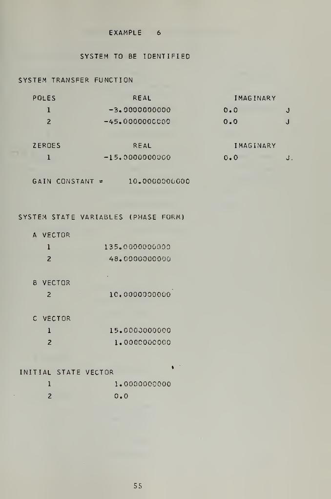
EXAMPLE 6
SYSTEM TO BE IDENTIFIED
SYSTEM TRANSFER FUNCTION
POLES REAL
1 -3.0000000000
2 -45.000000CC0C
ZEROES REAL
1 -15.0000000000
GAIN CONSTANT = 10.0000000000
SYSTEM STATE VARIABLES (PHASE FORM)
A VECTOR
1 13 5.0 000000000
2 48.0000000000
B VECTOR
2 10.0000000000
C VECTOR
1 15.0000000000
2 l.OOOCOOCOOO
INITIAL STATE VECTOR
1 1.0000000000
2 0.0
IMAGINARY
0.0 J
0.0 J
IMAGINARY
0.0 J
55

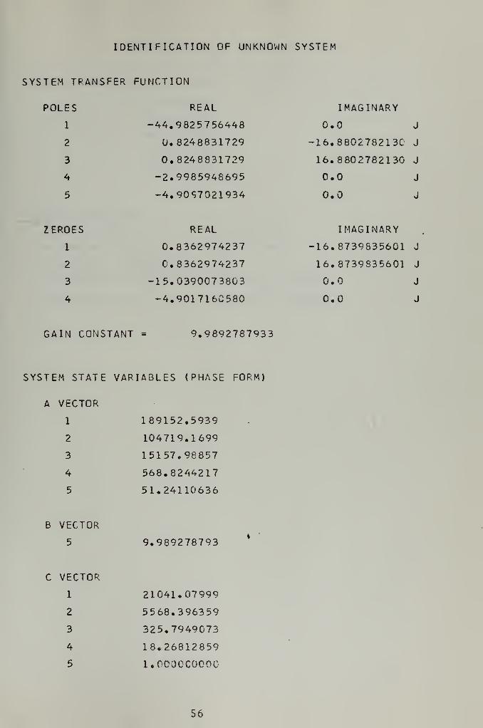
IDENTIFICATION OF UNKNOWN SYSTEM
SYSTEM TRANSFER FUNCTION
POLES REAL
1 -44.9825756448
2 0.8248831729
3 0.8248831729
4 -2.9985948695
5 -4.9097021934
ZEROES REAL
1 0.8362974237
2 0.8362974237
3 -15.0390073803
4 -4.901716C580
GAIN CONSTANT = 9.9892787933
SYSTEM STATE VARIABLES (PHASE FORM)
A VECTOR
1 189152.5939
2 104719.1699
3 15157.98857
4 568.8244217
5 51.24110636
B VECTOR
5 9.989278793
C VECTOR
1 21041.07999
2 5568.396359
3 325.7949073
4 18.26812859
5 l.OCOOCOOOC
IMAGINARY
0.0 J
16.8802782130 J
16.8802782130 J
0.0 J
0.0 J
IMAGINARY
16.8739835601 J
16.8739835601 J
0.0 J
0.0 J
56

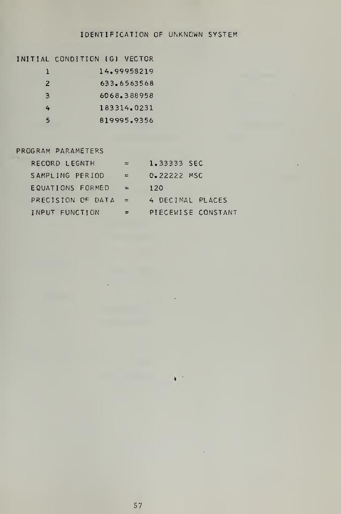
IDENTIFICATION OF UNKNOWN SYSTEM
INITIAL CONDITION (G) VECTOR
1 14,99958219
2 633.6563568
3 6068.388958
4 183314.0231
5 819995.9356
PROGRAM PARAMETERS
RECORD LEGNTH
SAMPLING PERIOD
EQUATIONS FORMED
PRECISION OF DATA
INPUT FUNCTION
1.33333 SEC
0.22222 MSC
120
4 DECIMAL PLACES
PIECEWISE CONSTANT
57

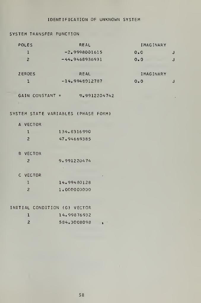
IDENTIFICATION OF UNKNOWN SYSTEM
SYSTEM TRANSFER FUNCTION
POLES REAL IMAGINARY
1 -2,9998001615 0.0 J
2 -44,9468936931 0.0 J
ZEROES REAL IMAGINARY
1 -14.9948012787 0.0 J
GAIN CONSTANT = 9.9912204742
SYSTEM STATE VARIABLES (PHASE FORM)
A VECTOR
1 134.8316990
2 47.94669385
B VECTOR
2 9.991220474
C VECTOR
1 14.99480128
2 1.000000000
INITIAL CONDITION (G) VECTOR
1 14.99876932
2 584.3008098 »
58


EXAMPLE
SYSTEM TO BE IDENTIFIED
SYSTEM TRANSFER FUNCTION
POLES REAL
1 -1.0000000000
2 -1.0000000000
3 -50.0C000C0000
ZEROES REAL
1 -5.0CCO00C0CO
2 -2O.00CCOO0000
IMAGINARY
l.COCCOOCOOO J
1.0000000000 J
0.0 J
IMAGINARY
0.0 J
0.0 J
GAIN CONSTANT = 5.0000000COC
SYSTEM STATE VARIABLES (PHASE FORM)
A VECTOR
1 100.0000000000
2 102.0000000000
3 52.0C00C0CCC0
B VECTOR
3 5.0000000000
C VECTOR
1 100.00000CG00C*
2 25.0000000000
3 l.OOCOOCOOOO
INITIAL STATE VECTOR
1 2.0000000000
2 1.0000000000
3 G.O
59

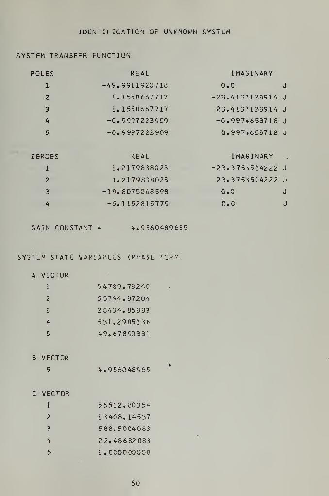
IDENTIFICATION OF UNKNOWN SYSTEM
SYSTEM TRANSFER FUNCTION
POLES REAL
1 -49,9911920718
2 1.1558667717
3 1.1558667717
4 -C. 9997223909
5 -0.9997223909
ZEROES REAL
1 1.2179838023
2 1.2179838023
3 -19.8075068598
4 -5.1152815779
GAIN CONSTANT = 4.9560489655
SYSTEM STATE VARIABLES (PHASE FORM)
A VECTOR
1 54789.78240
2 55794.37204
3 28434. 85333
4 531.2985138
5 49.67890331
B VECTOR
5 4.956048965
C VECTOR
1 55512. 80354
2 13408. 14537
3 588.5004083
4 22.48682083
5 l.CCOO 00000
IMAGINARY
0.0 J
23.4137133914 J
23.4137133914 J
-C. 9974653718 J
0.9974653718 J
IMAGINARY
23.3753514222 J
23.3753514222 J
0.0 J
0.0 J
60


IDENTIFICATION OF UNKNOWN SYSTEM
INITIAL CONDITION (G) VECTOR
1 225.0001273
2 10975.84397
3 117558.8284
4 6270060.545
5 11259586.57
PROGRAM PARAMETERS
RECORD LEGNTH
SAMPLING PERIOD
EQUATIONS FORMED
PRECISION OF DATA
INPUT FUNCTICN
1.20000 SEC
0.20000 MSC
120
4 DECIMAL PLACES
PIECEWISE CONSTANT
61

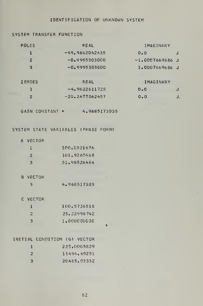
IDENTIFICATION OF UNKNOWN SYSTEM
SYSTEM TRANSFER FUNCTION
POLES REAL
1 -49,9862042435
2 -0.9995303000
3 -0.9995303C00
ZEROES REAL
1 -4.9622611725
2 -20.2677062457
GAIN CONSTANT = 4.9685173035
SYSTEM STATE VARIABLES (PHASE FORM)
A VECTOR
1 100.0021676
2 101.9260468
3 51.98526484
B VECTOR
3 4.968517303
C VECTOR
1 100.5736518
2 25.22996742
3 l.OOOCOOGOC
INITIAL CONDITION (G) VECTOR
1 225.00G5829
2 11494.69251
3 20485.03332
IMAGINARY
0.0 J
1.0007669686 J
1.0007669686 J
IMAGINARY
0.0 J
0.0 J.
62

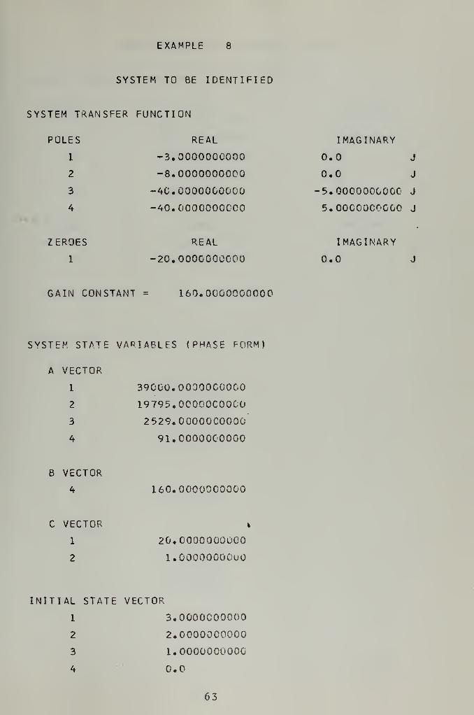
EXAMPLE 8
SYSTEM TO BE IDENTIFIED
SYSTEM TRANSFER FUNCTION
POLES REAL
1 -3.0000000000
2 -8,0000000000
3 -40.0000000000
4 -40.0000000000
ZEROES REAL
1 -20.0000G0CC00
IMAGINARY
0.0 J
0.0 J
5.0000000000 J
5.00C00C0G00 J
IMAGINARY
0.0 J
GAIN CONSTANT = 160.0000000000
SYSTEM STATE VARIABLES (PHASE FORM)
A VECTOR
1 39000. OOOOOCOOCO
2 19795. OOOOOCOOCO
3 2529.00000C0000
4 91. OOOOOCOOCO
B VECTOR
4 160.0000000000
C VECTOR
1 20.0000000U00
2 l.OOOOOOOOUO
INITIAL STATE VECTOR
1 3.0000000000
2 2.0000000000
3 1.0000000000
4 0.0
63

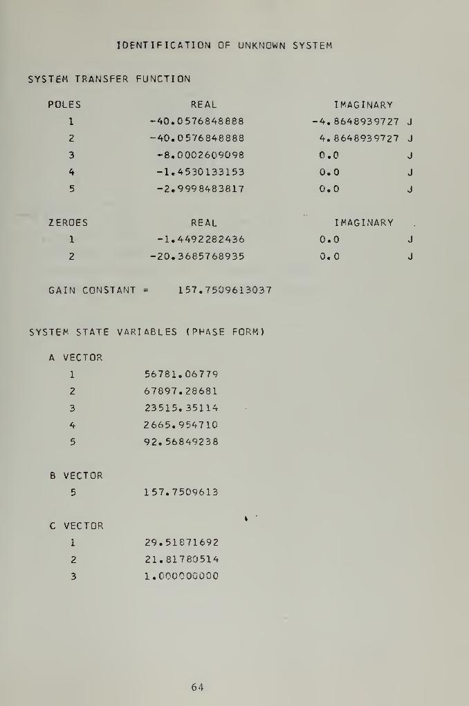
IDENTIFICATION OF UNKNOWN SYSTEM
SYSTEM TRANSFER FUNCTION
POLES REAL
1 -40.0576848888
2 -40.0576848888
3 -8.0002609098
4 -1.4530133153
5 -2.9998483817
ZEROES REAL
1 -1.4492282436
2 -20.3685768935
GAIN CONSTANT = 157.7509613037
SYSTEM STATE VARIABLES (PHASE FORM)
A VECTOR
1 56781.06779
2 67897.28681
3 23515.35114
4 2665.954710
5 92.56849238
B VECTOR
5 157.7509613
C VECTOR
1 29.51871692
2 21.81780514
3 l.COOOOOOOO
IMAGINARY
4.8648939727 J
4. 8648939727 J
0.0 J
0.0 J
0.0 J
IMAGINARY
0.0 J
0.0 J
64


IDENTIFICATION OF UNKNOWN SYSTEM
INITIAL CONDITION (G) VECTOR
1 62.00108720
2 5780.206688
3 169108.2337
4 1409764.537
5 1708815.026
PROGRAM PARAMETERS
RECORD LEGNTH
SAMPLING PERIOD
EQUATIONS FORMED
PRECISION OF DATA
INPUT FUNCTION
1.48842 SEC
0.24807 MSC
120
5 DECIMAL PLACES
PIECEWISE CONSTANT
65

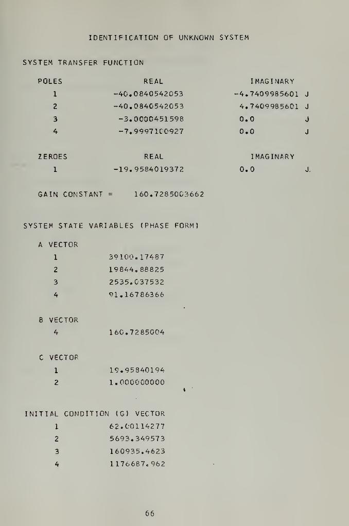
IDENTIFICATION OF UNKNOWN SYSTEM
SYSTEM TRANSFER FUNCTION
POLES REAL IMAGINARY
1 -40.0840542053 -4.7409985601 J
2 -40.0840542053 4.7409985601 J
3 -3.0000451598 0.0 J
4 -7.99971C0927 0.0 J
ZEROES REAL IMAGINARY
1 -19.9584019372 0.0 J.
GAIN CONSTANT = 160.7285003662
SYSTEM STATE VARIABLES (PHASE FORM)
A VECTOR
1 39100.17487
2 19844.88825
3 2535.037532
4 91.16786366
B VECTOR
4 160.7285004
C VECTOR
1 19.95840194
2 l.OOOOCOOOO
INITIAL CONDITION (G) VECTOR
1 62.00114277
2 5693.349573
3 160935.4623
4 1176687.962
66


EXAMPLE 9
SYSTEM TO BE IDENTIFIED
SYSTEM TRANSFER FUNCTION
POLES REAL
1 -1.0000000000
2 -5.0000000000
ZEROES REAL
GAIN CONSTANT = 10.000000000C
SYSTEM STATE VARIABLES (PHASE FORM)
A VECTOR
1 5.0000000000
2 6.0000000000
B VECTOR
2 10.0000000000
C VECTOR
1 l.OOQOOCOOOO
INITIAL STATE VECTOR
1 l.OOOOOGOOOO
2 0.0
IMAGINARY
0.0 J
0.0 J
IMAGINARY
67

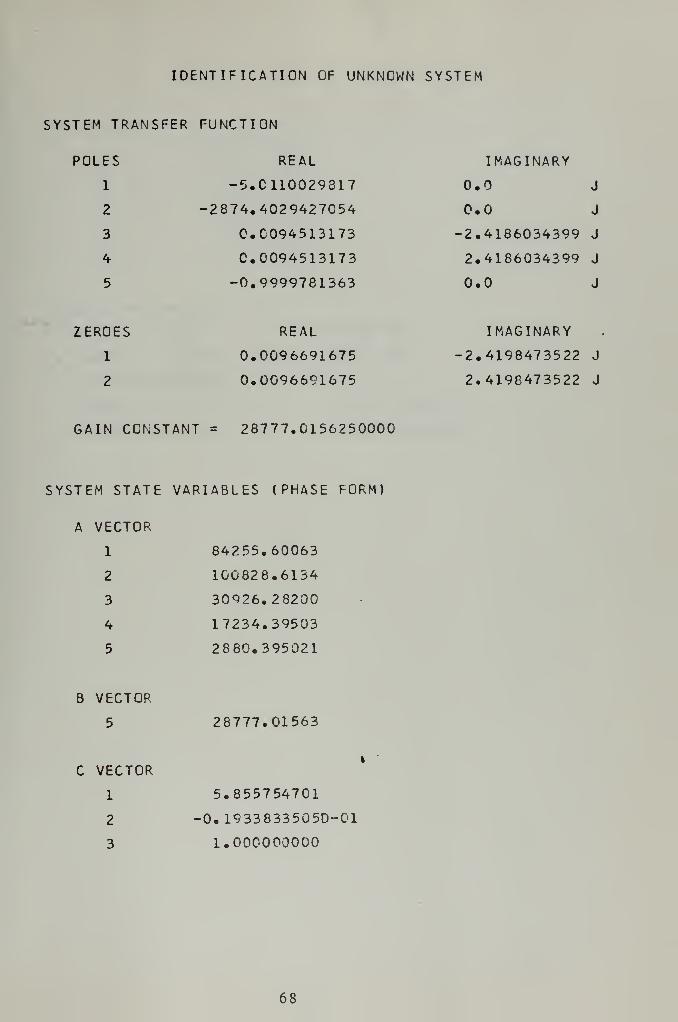
IDENTIFICATION OF UNKNOWN SYSTEM
SYSTEM TRANSFER FUNCTION
POLES REAL
1 -5.C110029317
2 -2874.4029427054
3 0.C094513173
4 C. 0094513173
5 -0.9999781363
ZEROES REAL
1 0.009 6691675
2 0.0096691675
GAIN CONSTANT = 28777.0156250000
SYSTEM STATE VARIABLES (PHASE FORM)
A VECTOR
1 84255.60063
2 100828.6134
3 30926.28200
4 17234.39503
5 2880.395021
B VECTOR
5 28777.01563
C VECTOR
1 5.855754701
2 -0. 1933833505D-01
3 1.000000000
IMAGINARY
0.0 J
0.0 J
-2.4186034399 J
2.4186034399 J
0.0 J
IMAGINARY
-2.4198473522 J
2.4198473522 J
68


IDENTIFICATION OF UNKNOWN SYSTEM
INITIAL CONDITION (G) VECTOR
1 1,450317645
2 2876.228032
3 17252.85740
4 16462.65716
5 101232.6568
PROGRAM PARAMETERS
RECORD LEGNTH = 12.00000 SEC
SAMPLING PERIOD = 2.000C0 MSC
EQUATIONS FORMED = 120
PRECISION OF DATA = 5 DECIMAL PLACES
INPUT FUNCTION = PIECEWISE CONSTANT
69

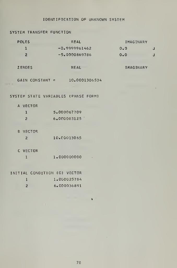
IDENTIFICATION OF UNKNOWN SYSTEM
SYSTEM TRANSFER FUNCTION
POLES REAL
1 -0,9999961462
2 -5.0000869786
ZEROES REAL
GAIN CONSTANT = 10.0001306534
SYSTEM STATE VARIABLES (PHASE FORM)
A VECTOR
1 5.000067709
2 6.000083125
B VECTOR
2 10.00013065
C VECTOR
1 1.000000000
INITIAL CONDITION (G) VECTOR
1 1.000025784
2 6.000036891
IMAGINARY
0.0 J
0.0 J
IMAGINARY
70

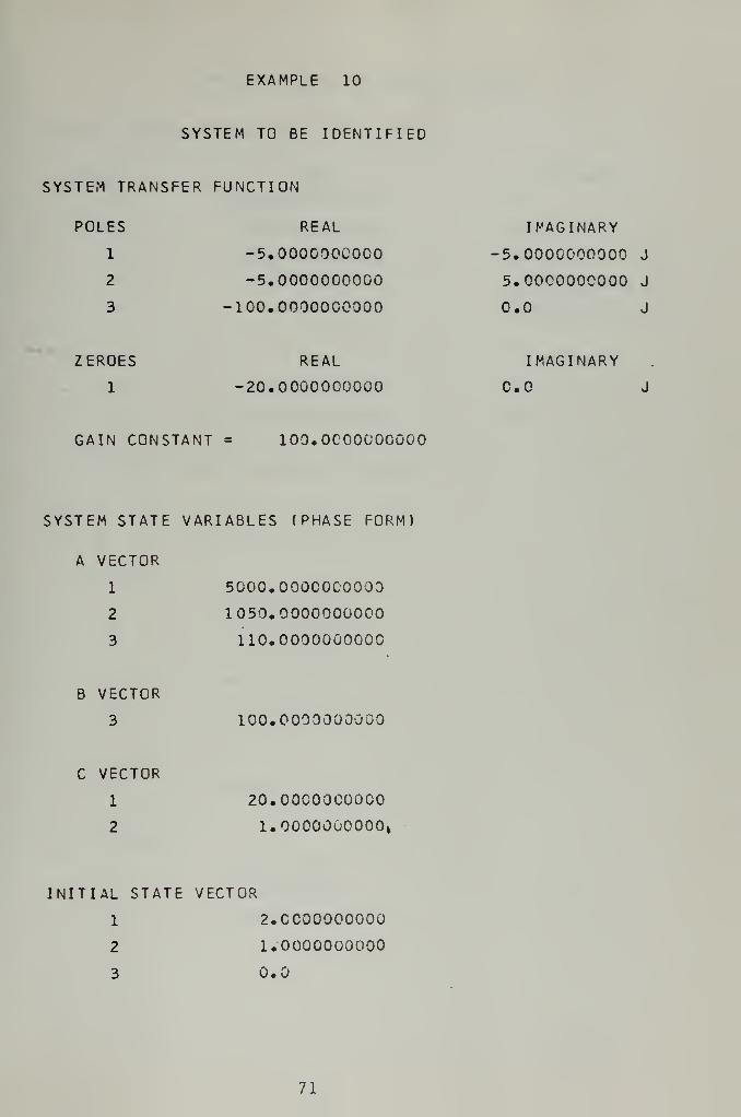
EXAMPLE 10
SYSTEM TO BE IDENTIFIED
SYSTEM TRANSFER FUNCTION
POLES REAL
1 -5,0000000000
2 -5.0000000000
3 -100.0000000000
ZEROES REAL
1 -20.0000000000
GAIN CONSTANT = 100. OCOOOOOOOO
SYSTEM STATE VARIABLES (PHASE FORM)
A VECTOR
1 50O0.0OOCOCO000
2 1050.0000000000
3 110.0000000000
B VECTOR
3 100.0000000000
C VECTOR
1 20.00C00C0000
2 U0000000000»
INITIAL STATE VECTOR
1 2. OCOOOOOOOO
2 1.0000000000
3 0.0
IMAGINARY
5.0000000000 J
5.0000000000 J
0.0 J
IMAGINARY
CO J
71


IDENTIFICATION OF UNKNOWN SYSTEM
SYSTEM TRANSFER FUNCTION
POLES REAL
1 3533,8075084749
2 -25.9614103219
3 -100.0395044818
4 -4.9998977161
5 -4.9998977161
ZEROES REAL
1 -19.5630088534
2 -26.9189879242
GAIN CONSTANT =-348 534.3750000000
SYSTEM STATE VARIABLES ( PHASE FORM)
A VECTOR
1 -458893162.9
2 -113910225.2
3 -13774844.37
4 -476693.1811
5 -3397.806798
B VECTOR
5 -348534.3750
C VECTOR
1 526.6163991
2 46.48199678
3 1.000000000
IMAGINARY
0.0 J
0.0 J
0.0 J
5.0000893933 J
5.000G893933 J
IMAGINARY
CO J
0.0 J
72


IDENTIFICATION OF UNKNOWN SYSTEM
INITIAL CONDITION (G) VECTOR
1 40.97649863
2 -139289.1252
3 -19623611.76
4 -535751377.4
5 -3138782043.
PROGRAM PARAMETERS
RECORD LEGNTH
SAMPLING PERIOD
EQUATIONS FORMED
PRECISION OF DATA
INPUT FUNCTION
0.600CC SEC
G.10CC0 MSC
120
5 DECIMAL PLACES
PIECEWISE CONSTANT
73

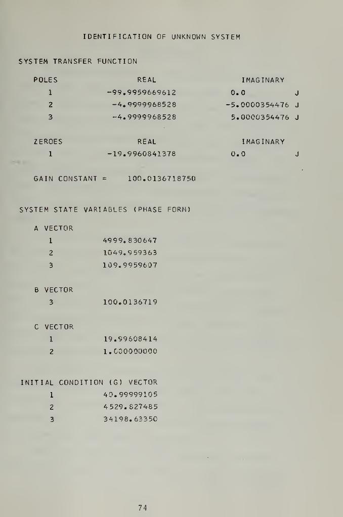
IDENTIFICATION OF UNKNOWN SYSTEM
SYSTEM TRANSFER FUNCTION
POLES REAL
1 -99.9959669612
2 -4,9999968528
3 -4,9999968528
ZEROES REAL
1 -19.9960841378
GAIN CONSTANT = 100,0136718750
SYSTEM STATE VARIABLES (PHASE FORM)
A VECTOR
1 4999.83C647
2 1049.959363
3 109.9959607
B VECTOR
3 100.0136719
C VECTOR
1 19.99608414
2 l.COOOOOOOO
INITIAL CONDITION (G) VECTOR
1 40.99999105
2 4529.827485
3 34198. 6335C
IMAGINARY
0.0 J
5.0000354476 J
5.0000354476 J
IMAGINARY
0.0 J
74

IV. CONCLUSIONS
The method of multiple integrations is a practical
and flexible method for identifying lumped parameter,
linear, time invariant systems. Complete and accurate
identifications can be made on the basis of arbitrary in-
put-output records taken over a short time interval and
accurate to only three or four significant figures. The
computational requirements of the method are not exces-
sive. The procedure can be implemented by relying en-
tirely on subroutines which are available in most computer
center libraries.
At present the technique is limited to comparatively
low order systems. When the input-output records are good
to three or four significant digits the method will be
capable of identifying systems up to about fifth order.
This limitation is due primarily to the algorithm used to
solve the overdetermined set of linear equations. As
better algorithms become available it will be possible to
identify higher order systems.
The accuracy of an identification is usually compar-
able to the number of significant digits in the input-
output data. Accuracy depends to a lesser extent on the
sampling rate, the nature of the input function driving
the system, and the order of the system.
There are several areas where additional research
might prove fruitful. Since the input-output records must
75

be in sampled data form for the computer it might be prof-
itable to reformulate the identification procedure from a
sampled system standpoint. Standard techniques could be
used to convert the sampled system representation obtained
from the identification to a continuous system representa-
tion. The ability to identify sampled systems would be a
worthwhile extension of this method.
The method of multiple integrations may prove very
useful as a tool for approximating high order systems with
low order systems. Research could be done to determine
the quality of the approximations obtained using this
method.
76

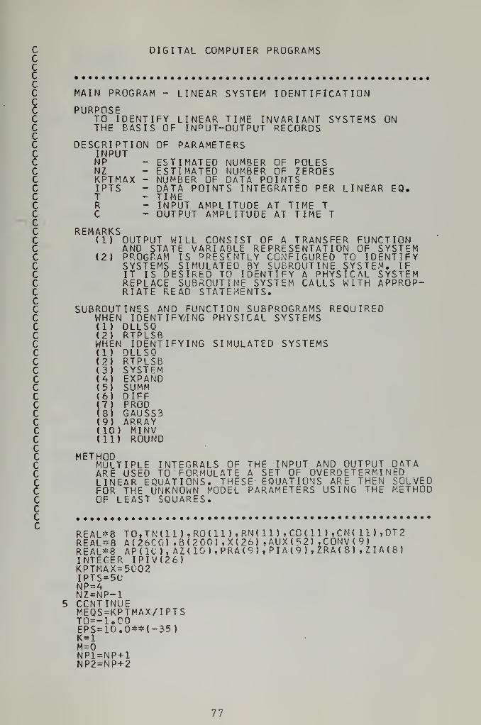
C DIGITAL COMPUTER PROGRAMSCCccC MAIN PROGRAM - LINEAR SYSTEM IDENTIFICATIONCC PURPOSEC TO IDENTIFY LINEAR TIME INVARIANT SYSTEMS ONC THE BASIS OF IN^UT-OUTPUT RECORDSCC DESCRIPTION OF PARAMETERSC INPUTC NP ESTIMATED NUMBER OF POLESC NZ ESTIMATED NUMBER OF ZEROESC KPTMAX - NUMBER OF DATA POINTSC IPTS - DATA POINTS INTEGRATED PER LINEAR EQ.C T TIMEC R INPUT AMPLITUDE AT TIME TC C OUTPUT AMPLITUDE AT TIME TCC REMARKSC (1) OUTPUT WILL CONSIST OF A TRANSFER FUNCTIONC AND STATE VARIABLE REPRESENTATION OF SYSTEMC (2) PROGRAM IS PRESENTLY CONFIGURED TO IDENTIFYC SYSTEMS SIMULATED BY SUBROUTINE SYSTEM. IFC IT IS DESIRED TO IDENTIFY A PHYSICAL SYSTEMC REPLACE SUBROUTINE SYSTEM CALLS WITH APPROP-C RIATE READ STATEMENTS.CC SUBROUTINES AND FUNCTION SUBPROGRAMS REQUIREDC WHEN IDENTIFY/ING PHYSICAL SYSTEMSC (1) DLLSQC (2) RTPLSBC WHEN IDENTIFYING SIMULATED SYSTEMSC (1) DLLSQC (2) RTPLSBC (3) SYSTEMC (A) EXPANDC (5) SUMMC (6) DIFFC (7) PRODC (8) GAUSS3C (9) ARRAYC (10) MINVC (11) ROUNDCC METHODC MULTIPLE INTEGRALS OF THE INPUT AND OUTPUT DATAC ARE USED TO FORMULATE A SET OF OVERDETE RMI NEDC LINEAR EQUATIONS. THESE EQUATIONS ARE THEN SOLVEDC FOR THE UNKNOWN MODEL PARAMETERS USING THE METHODC OF LEAST SQUARES.CCc
REAL*8 T0,TN(11) , R0U1 ),RN<11) , CO ( 1 1 ) »CN( 11) ,DT2REAL* 8 A(26C0) ,8(2 00)iX(26),AUX(52) ,C0NV(9)REAL*8 APIlt ), AZ(10),PRA(9),PIA(9),ZRA(8) , ZIA(8)INTEGER IPIV(26)KPTMAX=5C02IPTS=5CNP = 4NZ=NP-1
5 CONTINUEMEQS=KPTMAX/IPTST0=-1.C0EPS=10«0**<-35)K=lM=0NP1=NP+1NP2=NP+2
77

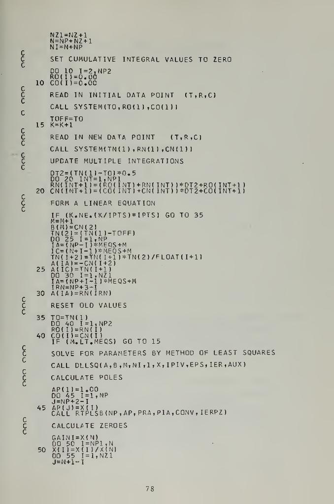
NZ1=NZ+1N=NP+NZ+1NI=N+NP
CC SET CUMULATIVE INTEGRAL VALUES TO ZEROC
C
C
DO 10 I=2,NP2RO(I)=0.00
10 CO(I)=O.OCcC READ IN INITIAL DATA POINT (T,R,C)
CALL SYSTEM(T0,R0(1) ,C0(1)
)
TOFF=TO15 K=K+1
CC READ IN NEW DATA POINT (T,R,C)C
CALL SYSTEM(TNd) tRN(l) iCN(l) )
CC UPCATE MULTIPLE INTEGRATIONSC
DT2=(TN( 1)-T0)*0.5DO 20 INT=1,NP1RN(INT+1 )=(R0( INT)+RN( INT) )*DT2+R0( INT+1
)
20 CN( INT+1 ) = ( CO ( INT)+CN( INT) )*DT2+C0( INT+1)CC FORM A LINEAR EQUATIONC
IF (K.NE.(K/IPTS)*IPTS) GO TO 35M = M+1B(M)=CN(2)TN(2)=(TN(1 )-TOFF)DO 25 1=1, NPI A=( NP-I )*MFOS+MIC=(N+I-1)*MEQS+MTN( I+2)=TN( 1+1 )*TN(2)/FL0AT( 1+1)A( IA)=-CN( 1+2)
25 A( IC)=TN(I+1)DO 30 1=1, NZ1IA=(NP+I-1 )*MEQS+MIRN=NP+3-I
30 A( IA)=RN(IRN)CC RESET OLD VALUESC
35 T0=TN(1
)
DO 40 1=1, NP2R0( I )=RN( I
)
40 COU ) = CN(I )
IF (M.LT.MEQS) GO TO 15CC SOLVE FOR PARAMETERS BY METHOD OF LEAST SQUARESC
CALL DLLSQ(A,B,M,NI,1,X,IPIV,EPS, IER,AUX)CC CALCULATE POLESC
AP(1)=1.C0DO 45 1=1, NPJ=NP+2-I
45CALL
J
RTPLSB(NP,AP,PRA,PIA,CONV,IERPZ)CC CALCULATE ZEROES
GAINI=X(N)DO 50 I=NP1,N
50 X( I )=X( I )/X(N)DO 55 1=1, NZ1J=N+1-I
78


ccc
55
60
65
7075
80
85
90
9009019029039049059069079C8909910911
912913914915916917918919920921
AZ(I)=X( J)IF (NZ.EQ.O) GO TO 60££LL RTPLSB<NZ,AZ,ZRA t ZIA,CONV,IERPZ)CONTINUE
1
OUTPUT
WRITE(6WRITE(6WRITE(6WRITE(6WRITE(6WRITE(6WRITE(6WRITE(6WRITE(6WRITE(6WRITE(6DO 65 I
WRITE(6CONTINUWRITE(6IF (NZ.DO 70 I
WRITERCONTINUCONTINUWRITE(6WRITE(6WRITE(6DO 80 I
II=NP+2WRITE(6CCNTINUWRITE(6WRTJE (
*
WRITE (6DO 85 I
II=NZ+2WRITE(6CCNTINUWRITE(6DO 90 I
II=N+IWRITE(6CONTINUGO TO 5FORMAT
(
FORMAT(FORMAT
(
FORMAT
(
FORMAT
(
FORMAT
(
FORMAT(FORMAT
(
FORMAT(FORMAT(FORMAT
(
FORMAT
(
E16.8,/FORMAT!FORMAT
(
FORMAT
(
FORMAT(FORMAT(FORMAT
(
FORMAT
(
FORMAT(FORMAT
(
FORMAT(STOPEND
914)915)916)917)918)919)920)921)900)901 )
902)1,NP903)
KMIPTSEPSAUX(l)IER( IPIV( I) ,I=1,NI
)
I,PRA( I) ,PIA(I )
904)Q.O) GO TO 75ltNZ903) I,ZRA(I) ZIA(I)
905) GAINI906)907)1,NP•I
910) I , AP( I I
)
90 8)910) NP. GAINI909)
: 1,NZ1•I
910) I , AZ( I I
)
913): 1,NP
,^10)E
I » X( I I )
1H1,///t//tl17X T
//tl//tl//////tl//tl//,117X,1H ,
t9X T
//t5//,1////15X»15X,15X,15X,15X,15X,15X,
///t12X,5X,'12,75X, •
5X,'tl2X5X, '
5X,'5X,«12,79X, '
1118X,4(5X,'//tl» NUM•NUM•DAT'EPS•RMS' IER• IPI
25X,'SYSPOLEX,G1ZEROGAIN, 'SYA VEb VEC VEX,G1IER')
E20.INIT2X, '
BERBERA PO
ERR
V( I )
t/t/
•IDENTITEM TRAS' , 12X,5.8,6X,ES' ,11XCONSTASTEM STCTOR',/CTOR'CTOR'5.8,/)tI5,5X,
9,5X) ,/IAL STAPROGRAMOF DATAOF EOUAINTS PE
= t
OR ='= i
= i
FICATION OF UNKNOWN SYSTEM')NSFER FUNCTION'
)
'REAL', 13 X,
•
IMAGINARY' ,/)G15.8,1X, 'J',/), 'REAL' ,13X,' IMAGINARY' ,/)NT =',G15.8,/)ATE VARIABLES (PHASE FORM)'))
)
)
•EPS' ,E15.8,5X, «AUX«,
/, 5X,4(E20.9,5X) ,//)TE VECTOR' ,/)PARAMETERS' ,/)POINTS =',I6,/)
TIONS =',I6,/)R EQUATION =• ,16,/)16.8,/)16.8,/)4,/)
tEtEt I
,15( 12, IX) ,/)
79


cc
,
cC SUBROUTINE SYSTEMCC PURPOSEC GENERATES INPUT-OUTPUT RECORDS FOR IDENTIFICA-C TION PROGRAM BY SIMULATING A SYSTEM DESCRIBEDC BY A TRANSFER FUNCTION THAT IS READ INCC USAGEC CALL SYSTEM(T,R,C)CC DESCRIPTION OF PARAMETERSC INPUTC NP NUMBER OF POLESC P(I) - THE VECTOR OF POLESC NZ NUMBER OF ZEROESC Z(I) - THE VECTOR OF ZEROESC GAIN - THE GAIN CONSTANTC OUTPUTC T TIMEC R INPUT AMPLITUDE AT TIME TC C OUTPUT AMPLITUDE AT TIME TCC REMARKSC (1) INPUT FUNCTION MAY BE CHANGED BYC CHANGING ONE CARD IN PROGRAMC (2) R AND C ARE ROUNDED TO MA DIGITSC (3) ALL FLOATING POINT VARIABLES ARE DECLAREDC DOUBLE PRECISION (REAL*8).CC SUBROUTINES AND FUNCTION SUBPROGRAMS REQUIREDC (1) SUMMC (2) DIFFC (3) PPODC (4) EXPANDC (5) GAUSS3C (6) ARRAYC (7) MINVC (8) ROUNDCC METHODC TRANSFER FUNCTION IS CONVERTED TO STATEC VARIABLE REPRESENTATION AND INTEGRATED USINGC TRAPEZOIDAL INTEGRATIONCCc
c
SUBROUTINE SYSTEM( T , R, C
)
CREAL*8 AA( 1G),CC(1C) ,A(9,9) ,R(9,1) ,XXX(9,9)REAL*8 PHI (9,9) ,DEL(9, 1) , XX ( 9 , 1 ) , UU( 1 , 1 )
REAL* 8 T,R,C,U,DT,AI(9,9),ZZZ(9,9)CCMPLEX#16 P(9) ,Z( 8)
CIF (T.GE.O.OO) GO TO 55
CC INPUT POLES, ZEROES, AND GAIN CONSTANT
READ(5,899,END=999) NPREAD(5,898) ( P ( I ) ,
I =1 , NP
)
CALL EXPAND (NP,P,AA)DO 5 1=1, NPCC( I )=0.00
5 CONTINUEREAD(5,899) NZIF (NZ.EQ.O) GO TO 10READ(5,898) ( Z ( I ) , 1=1 , NZ
)
CALL EXPAND <NZ,Z,CC)10 CONTINUE
READ(5,898) GAIN
80

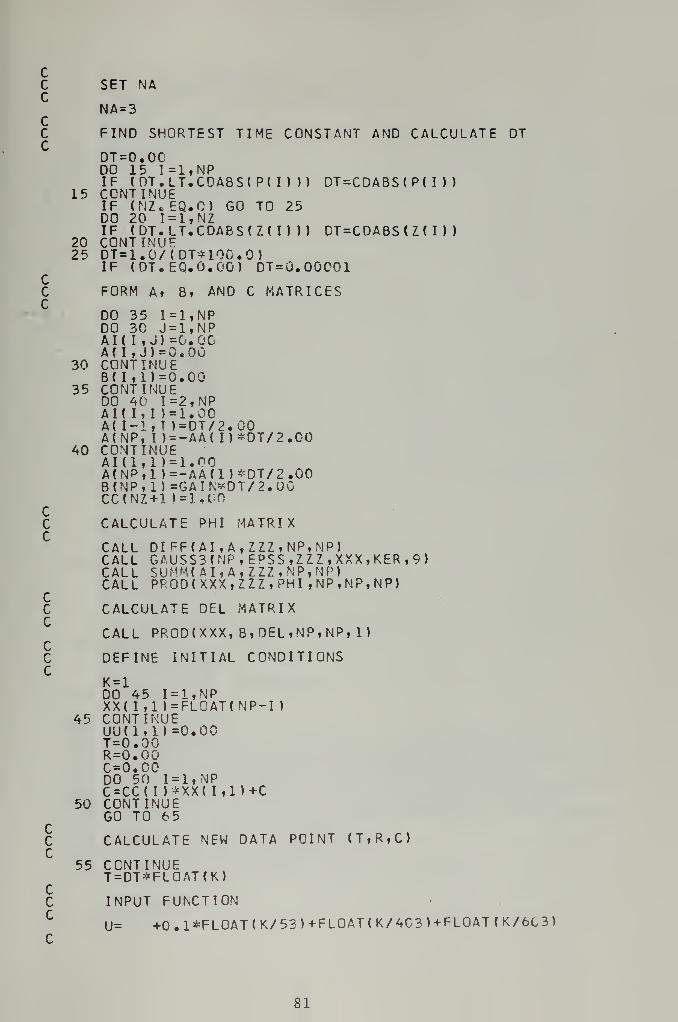
cC SET NAC
ccc
NA=3CC FIND SHORTEST TIME CONSTANT AND CALCULATE DT
DT=O.OCDO 15 1=1, NPIF (DT.LT.CDABS(Pd) )) DT =CDABS ( P ( I ) )
15 CONTINUEIF (NZ. EQ.C) GO TO 25DO 20 1=1, NZIF (DT.LT.CDABS(ZU) )) DT =CDABS ( Z ( I ) )
20 CONTINUE25 DT=1.0/(DT*10C.O)
IF (DT.EQ.O.CO) DT=G.00C01CC FORM A, B, AND C MATRICESC
DO 35 1=1, NPDO 30 J=1,NPAid, J) -0.00A( I, J)=0.00
30 CONTINUEB(I ,1)=0.00
35 CONTINUEDO 40 I=2,NPAU I, I) = 1.00A( 1-1, I )=DT/2.00A(NP, I )=-AA( I >*DT/2.00
40 CONTINUEAI ( 1 , 1 ) = 1.00A(NP,1 )=-AA(l)*DT/2.00B(NP, 1)=GAIN*DT/2.0CCCINZ+1 1 = 1.CO
CC CALCULATE PHI MATRIXC
CALL DIFF(AI,A,ZZZ,NP,MP)CALL GAUSS3(NP, EPSS ,ZZZ , XXX , KER ,9
)
CALL SUMM(AI,A,ZZZ,NP,NP)CALL PROD ( XXX, ZZZ, PHI ,NP,MP,NP)
CC CALCULATE DEL MATRIXC
CALL PRODtXXX, B, DEL ,NP, NP, 1
)
CC DEFINE INITIAL CONDITIONSC
K = lDO 45 1=1, NPXX( 1,1 )=FLOAT( NP-I
)
45 CONTINUEUU(lt 1) =0.00T=0.00R=0.00C=0.00DO 50 1=1, NPC=CC( I )*XX( I,l)+C
50 CONTINUEGO TO 65
CC CALCULATE NEW DATA POINT (T,R,C)C
55 CONTINUET=DT#FLOAT(K)
CC INPUT FUNCTION
U= +0.1*FL0AT<K/53)+FL0AT(K/4C3)+FL0AT(K/60 3)
81

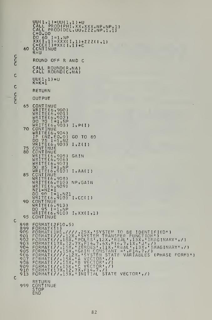
UU(1,1 )=UU(1,1 )+UCALL PR0D(PHI,XX,XXX,NP,NP,1)CALL PR0D(DEL,UU,ZZZ,NP,1,1)C=0.00DO 60 1=1, NPXX(I,1)=XXX( I,1)+ZZZU ,1)C=CC( I )*XX( 1,1 J+C
60 CONTINUER=U
CC ROUND OFF R AND CC
CALL ROUND(R,NA)CALL ROUND(CtNA)
UU(1,1)=UK=K + 1
CRETURN
CC OUTPUTC
65 CONTINUEWRITE(6,900)WRITE(6 f 901)WRITE(6,902)DO 70 1=1, NPWRITE<6,903) I,P(I)
70 CONTINUEWRITE(6,904)IF (NZ.EQ.O) GO TO 80DO 75 1=1, NZWRITE(6,903J I , Z ( I )
75 CONTINUE80 CONTINUE
WRITE (6, 905) GAINWRITE(6,906)WRITE(6,907)DO 85 1=1, NPWRITE(6,910J I,AA(I)
85 CONTINUEWRITE(6,908)WRITE(6,?10) NP,GAINWRITE(6,909)NZ1=NZ+1DO 90 1=1, NZ1WRITE(6,910) I,CC(I)
90 CONTINUEWRITE(6,913)DO 95 1=1, NPWRITE(6,910) I,XX(I,1)
95 CONTINUE
898 FORMAT(2F10.5)899 FORMAT(Il)900 FORMAT* 1H1 ,////, 25X , 'SYSTEM TO BE IDENTIFIED')901 FCRMAT(///, 12X, ' SYSTEM TRANSFER FUNCTION')902 FORMAT (//,15X, • POLES' , 12X, • REAL • , 13X ,
• IMAGINARY' ,/)9 03 F0RMAT(17X,I2,7X,F]4.7,6X,Fl^ e 7,lX,'J',/)904 FORMAT (//,15X, ' ZEROES «, 1 IX ,« R EAL ', 1 3X ,
•
IMAGINARY' ,/)905 FORMAT ( //,15X, 'GAIN CONSTANT =',F14.7,/)906 F0RMAT(////,12X, 'SYSTEM STATF VARIABLES (PHASE FORM)')907 FCRMAT(//,15X, ' A VECTOR',/)908 FCRMAT( //,15X, »B VECTOR',/)909 FGRMAT(//, 15X, «C VECTOR',/)910 F0RMAT(17X,I2,7X,F14.7,/)913 F0RMAT(//,15X,
•
INITIAL STATE VECTOR',/)
RETURN999 CONTINUE
STOPEND
82

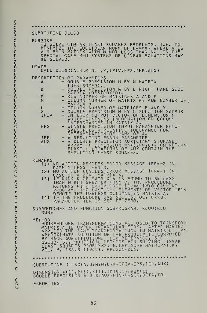
cccC SUBROUTINE DLLSQCC PURPOSEC TO SOLVE LINEAR LEAST SQUARES PROBLEMS, I.E. TOC MINIMIZE THE EUCLIDEAN NORM OF B-A*X, WHERE A ISC A M BY N MATRIX WITH M NOT LESS THAN N. IN THEC SPECIAL CASE M=N SYSTEMS OF LINEAR EQUATIONS MAYC BE SOLVED.CC USAGEC CALL DLLSQ( A ,B ,M ,N , L , X, I PI V, EPS, I ER, AUX
)
CC DESCRIPTION OF PARAMETERSC A DOUBLE PRECISION M BY N MATRIXC (DESTROYED).C B DOUBLE PRECISION M BY L RIGHT HAND SIDEC MATRIX (DESTROYED).C M ROW NUMBER OF MATRICES A AND BC N COLUMN NUMBER OF MATRIX A, ROW NUMBER OFC MATRIX XC L COLUMN NUMBER OF MATRICES B AND XC X DOUBLE PRECISION N BY L SOLUTION MATRIXC IPIV - INTEGER OUTPUT VECTOR OF DIMENSION NC WHICH CONTAINS INFORMATION CN COLUMNC INTERCHANGES IN MATRIX A.C EPS - SINGLE PRECISION INPUT PARAMETER WHICHC SPECIFIES A RELATIVE TOLERANCE FORC DETERMINATION OF RANK OF A.C IER - A RESULTING ERROR PARAMETERC AUX - A DOUBLE PRECISION AUXILIARY STORAGEC ARRAY OF DIMENSION MAX(2*N,L). ON RETURNC FIRST L LOCATIONS OF AUX CONTAIN THEC RESULTING LEAST SQUARES.CC REMARKSC (1) NO ACTION BESIDES ERROR MESSAGE IER=-2 INC CASE M LESS THAN N.C (2) NO ACTION BESIDES ERROR MESSAGE IER=-1 INC CASE OF A ZERO MATRIX A.C (3) IF RANK K OF MATRIX A IS FOUND TO BE LESSC THAN N BUT GREATER THAN 0, THE PROCEDUREC RETURNS WITH ERROR CODE IEP = K INTO CALLINGC PROGPAM. THE LAST N-K ELEMENTS OF VECTOR IPIVC DENOTE THE USELESS COLUMNS IN MATRIX A.C (4) IF THE PROCEDURE WAS SUCCESSFUL, ERRORC PARAMETER IER IS SET TO ZERO.CC SUBROUTINES AND FUNCTION SUBPROGRAMS REQUIREDC NONECC METHODC HOUSEHOLDER TRANSFORMATIONS ARE USED TO TRANSFORMC MATRIX A TO UPPER TRIANGULAR FORM. AFTER HAVINGC APPLIED THE SAME TRANSFORMATIONS TO MATRIX B, ANC APPROXIMATE SOLUTION OF THE PROBLEM IS COMPUTEDC BY BACK SUBSTITUTION. FOR REFE^ANCE, SEEC GOLUB, G., NUMERICAL METHODS FOR SOLVING LINEARC LEAST SQUARES PROBLEMS, NUMEPISCHE MATHEMATIK,C VOL. M, ISS.3 (1965), PP. 206-216.CCr
SUBROUTINE DLL SQ(A,B,M,N,L,X, IPIV, EPS, IER, AUX)
DIMENSION A(1),B(1) ,X(l),IPiy(l),AUX(l)DOUBLE PRECISION A , B , X , AUX, P I V, H, S IG, BETA, TOL
CC ERROR TESTC
83

IF(M-N)30,1,1CC GENERATICN OF INITIAL VECTOR S(K) ( K=l , 2 , . . . , N)C IN STORAGE LOCATIONS AUX(K) ( K= 1 , 2, . . . , N)
1 PIV=C.D0IEND=0DC 4 K=1,NIPIV(K)=KH=O.DOIST=IEND+1IEND=IEND+MDO 2 1= 1ST, I END
2 H=H+A(I )*A(I)AUX(K)=HIF(H-PIV)4,4,3
3 PIV=HKPIV=K
4 CONTINUECC ERROR TESTC
IF(PIV)31,3L,5CC DEFINE TOLERANCE FOR CHECKING RANK OF A
5 SIG=DSQRT(PIV)TOL=SIG*ABS(EPS)
CCC DECOMPCSITICN LOOP
LP=L*MIST=-MDO 21 K=1,NIST=IST+M+1IEND=IST+M-KT ~KP P'-i^IF (1)8, 8,
6
CC INTERCHANGE K-TH COLUMN OF A WITH KPIV-TH IN CASEC KPIV.GT.K.
6 H=AUX(K)AUX(K)=AUX(KPIV)AUX(KPIV)=HID=I*MDO 7 I=IST,IENDJ=I+IDH=A( I
)
A(I )=A( J)7 A(J)=H
CC COMPUTATION OF PARAMETER SIG
8 IF(K-1)11,11,99 SIG^O.DO
DO 10 I=IST,IEND10 SIG=SIG+A( I)*A( I)
SIG=DSQRT(SIG)CC TEST ON SINGULARITY
IF( SIG-T0L)32,32,11CC GENERATE CORRECT SIGN OF PARAMETER SIG
11 H=A(IST)IF(H)12,13,13
12 SIG=-SIGCC SAVE INTERCHANGE INFORMATION
13 IPIV(KPIV)=IPIV(K)IPIV(K)=KPIV
CC GENERATION OF VECTOR UK IN K-TH COLUMN OF MATRIXC A AND OF PARAMETER BETA
BETA=H+SIG
84


cc
cc
cc
cccc
A(IST)=BETABETA=1.D0/(SIG*BETA)J = N+KAUX(J)=-SIGIF(K-N) 14,19,19
TRANSFORMATION OF MATRIX A14 PIV=O.DO
ID=CJST=K+1KPIV=JSTDO 18 J=JST,NID=ID+MH=0.D0DO 15 I=IST,IENDI 1 = 1 + 1
D
15 H=H+A( I )*A( II)H=BETA*HDO 16 I=IST,IENDII=I+ID
16 A(II)=A( II )-A( I)*H
UPDATING OF ELEMENT S(J) STORED IN LOCATION AUX(J)I 1= IST + IDH=AUX(J)~A( II)*A(II )
AUX( J)=HIF(H-PIV)18, 18,17
17 PIV=HKPIV=J
18 CONTINUE
TRANSFORMATION OF RIGHT HAND SIDE MATRIX B19 DO 21 J=K,LM,M
H=O.DOIEND=J+M-KI I=ISTDO 20 I=J,IENDH=H+A( I I )#B( I)
20 11=11+1H=BETA*HII=ISTDO 21 I=J,I ENDB(I ) = B( I )-A( II )*H
21 11=11+1END OF DECOMPOSITION LOOP
BACK SUBSTITUTION AND BACK INTERCHANGEIER=0I = NLN=L*NPIV*1«D0/AUX(2*N)DO 22 K=N,LN,NX(K)=PI V*B(I )
22 I=I+MIF(N-1 )26, 26,23
23 JST=(N-1)*M+NDO 2 5 J=2,NJST=JST-M-1K=N+N+1-JPIV=1.D0/AUX(K)KST=K-NID=IPIV(KST)-KSTIST=2-JDO 25 K=1,LH=B(KST)IST=IST+NIEND=IST+J-2II=JSTDO 24 I=IST,IENDII-II+M
24 H = H-A( I I )*X( I)
85

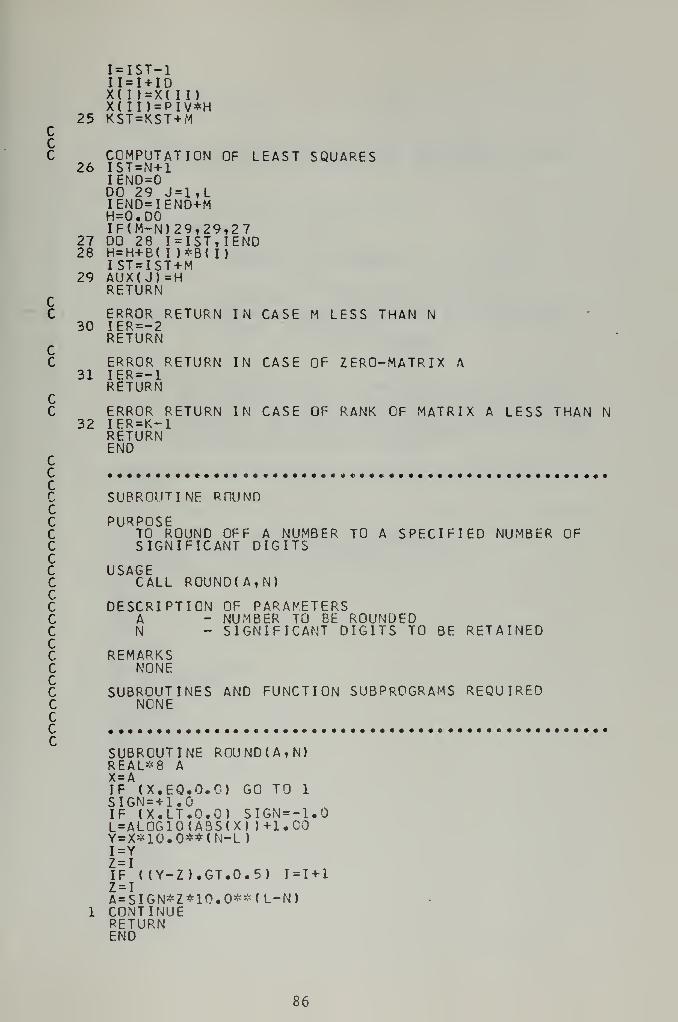
I=IST-11 1 = 1 + 1
D
X( I) = X( II)X( II)=PIV*H
25 KST=KST+MCcC COMPUTATION OF LEAST SQUARES
26 IST=N+1IEND=0DO 29 J=1,LIEND=IEND+MH=O.DOIF(M-N)29,29,27
27 DO 28 I=IST T IEND28 H=H+B( I )*B(I)
IST=IST+M29 AUX(J)=H
RETURNCC ERROR RETURN IN CASE M LESS THAN N
30 IER=-2RETURN
CC ERROR RETURN IN CASE OF ZERO-MATRIX A
31 IER=-1RETURN
CC ERROR RETURN IN CASE OF RANK OF MATRIX A LESS THAN N
32 IER=K-1RETURNEND
CccC SUBROUTINE ROUNDCC PURPOSEC TO ROUND OFF A NUMBER TO A SPECIFIED NUMBER OFC SIGNIFICANT DIGITSCC USAGEC CALL ROUND(A,N)CC DESCRIPTION OF PARAMETERSC A NUMBER TO BE ROUNDEDC N SIGNIFICANT DIGITS TO BE RETAINEDCC REMARKSC NONECC SUBROUTINES AND FUNCTION SUBPROGRAMS REQUIREDC NONECCc
SUBROUTINE ROUND(A,N)REAL*8 AX = AIF (X.EQ.O.O) GO TO 1
SI6N-+1.0IF (X.LT.O.C) SIGN=-1.0L=AL0G10(A3S(X) )+l.COY=X*10.0**(N-L )
I = YZ=IIF ( (Y-Z).GT.0.5) 1=1+1Z = I
A=SIGN*Z*10.0**(L-N)1 CONTINUE
RETURNEND
86

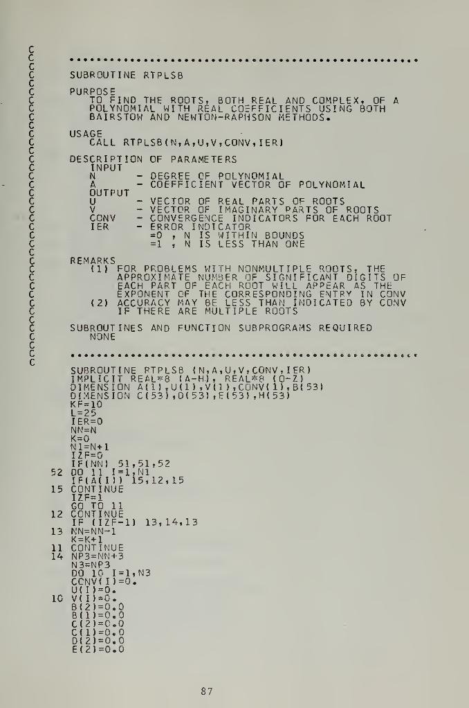
cc .
cC SUBROUTINE RTPLSBCC PURPOSEC TO FIND THE ROOTS, BOTH REAL AND COMPLEX, OF AC POLYNOMIAL WITH REAL COEFFICIENTS USING BOTHC BAIRSTOW AND NEWTON-RAPHSON METHODS.CC USAGEC CALL RTPLSB(N,A,U,V,CONV,IER)
C DESCRIPTION OF PARAMETERSC INPUTC N DEGREE CF POLYNOMIALC A COEFFICIENT VECTOR OF POLYNOMIALC OUTPUTC U VECTOR OF REAL PARTS OF ROOTSC V VECTOR OF IMAGINARY PARTS OF ROOTSC CONV - CONVERGENCE INDICATORS FOR EACH ROOTC IER - ERROR INDICATORC =0 t N IS WITHIN BOUNDSC =1 , N IS LESS THAN ONECC REMARKSC (1) FOR PROBLEMS WITH NONMULTIPLE ROOTS, THEC APPROXIMATE NUMBER OF SIGNIFICANT DIGITS OFC EACH PART OF EACH ROOT WILL APPEAR AS THEC EXPONENT OF THE CORRESPONDING ENTRY IN CONVC (2) ACCURACY MAY BE LESS THAN INDICATED BY CONVC IF THERE ARE MULTIPLE ROOTSCC SUBROUTINES AND FUNCTION SUBPROGRAMS REQUIREDC NONECc .,
cSUBROUTINE RTPLSB ( N, A , U, V, CONV , I ER
)
IMPLICIT REAL*8 (A-H), REAL*8 (O-Z)DIMENSION A(l) ,U(1 ) ,V(1 ) ,CONV( 1) , B( 53)DIMENSION C( 53) ,D( 53) ,E( 53) ,H( 53)KF=10L = 25IER =NN = NK=0N1=N+1IZF=0IF(NN) 51,51,52
52 DO 11 1=1, NlIF(AU)) 15,12,15
15 CONTINUEIZF=1GO TO 11
12 CONTINUEIF (IZF-1) 13,14,13
13 NN=NN-1K = K+1
11 CONTINUE14 NP3=NN+3
N3=NP3DO 10 1=1, N3CCNV( I )=0.U( I )=0.
10 V(I)=0.B(2)=0.0B(1)=0.0C(2)=C.OC(1)=0.0D(2)=0.0E(2)=0.0
87

H(2)=0.0DO 101 J=3,NP3H( J)=A( J+K-2)
101 CONTINUET=1.0SK=10.C**KF
150 IF(H(NP3)I 200,151,200151 U(NP3)=0.0
V(NP3)=0.C0NV(NP3)=SKNP3=NP3-1IF(NP3J 51,51,150
200 IF(NP3-3) 54,54,201201 PS=0.0
QS=0.0PT=0.0QT=0.0S=0.0REV=1.0SK=10.0**KFIF(NP3-4) 51,202,203
202 R=-H(4)/H(3)GO TO 500
2C3 DO 207 J=3,NP3IF(H( J) )204,207,204
204 S = S+DLOG(DABS(H( J) ) )
207 CONTINUEFPN1=N+1S=DEXP( S/FPN1 )
DO 208 J=3,NP3H( J)=H( J)/S
208 CONTINUEIF(DABS(H(4)/H(3) ) -DABS ( H ( NP3-1 ) /H( NP3 ) ) ) 2 5C , 2 52 , 252
2 50 CONTINUET=-TN-(NP3-4)/2 + 3DO 251 J = 3.MS=H( J)JJ=NP3-J+3H( J)=H( JJ)
251 H(JJ)=S252 IF(QS) 253,254,253253 CONTINUE
P=PSQ-QSGO TO 300
254 HH?=H(NP3-2)IF(HH2) 256,255,256
255 Q=1.0P=-2.0GG TO 257
256 Q=H(NP3)/HH2P=(H(NP3-1 )-Q*H(NP3-3) )/HH2
257 IF(NP3-5)258,55C,258258 R=0.0300 CONTINUE
DO 490 1=1,
L
DO 351 J=3,NP3B< J)=H( J)-P*B<J-l)-Q*BU-2)C( J) = B( J)-P*C( J-1)-Q*C( J-2)
351 CONTINUEIF(H(NP3-1) )352, 400,352
3 52 CONTINUEIF (3(NP3-1>) 353,400,353
3 53 AVHB1=DABS(H(NP3-1) /B(NP3-1 )
)
IF (AVHB1-SK) 45 0,354,354354 B(NP3)=H(NP3)-Q*B(NP3-2)400 IF(B(NP3) )401,550,401401 AVHB2=DABS(H(N D3)/B(NP3) )
IF(SK-AVHB2) 55 0,450,450450 DO 451 J=3,NP3
D( J)=H( J ) + R*D( J-l)
88


E(J)=D( J)+R*E( J-l)451 CONTINUE
IF(D(NP3))452,50O,452452 CONTINUE
AVHD3=DA3S(H(NP3)/D(NP3) )
IF (SK-AVHD3) 500,453,453453 CC2=C(NP3-2)
CC3=C(NP3-3)C(NP3-1 )=-P*CC2-Q*CC3CC1=C(NP3-1 )
S=CC2*CC2-CC1*CC3IF(S)455,454,455
454 CONTINUEP=P-2.00Q=Q*(Q+1.0)GO TO ^56
4 55 P=P+(B (NP3-1)*CC2-B(NP3)*CC3)/SQ=Q+(-B(NP3-l)~CCl+B(NP3)*CC2)/S
456 IF(E(NP3-1) )453,457,'457 R=R~1.C
GO TO 490458 R=R-D(NP3)/E(NP3-1)490 CONTINUE
PS = PTQS=QTPT = PQT = QIF(REV)49l,492,492
491 SK=SK/10.0492 REV=-REV
GO TO 250500 IF(T) 501,502,502501 R=1.0/R502 NP=NP3-3
U(NP)=R\MNP)*C ,0CGNV(NP)=SKNP3=NP3-1DO 503 J=3,NP3
503 H< J)=D( J)IF(NP3-3)300,51,300
5 50 IF(T) 551,552,552551 P=P/Q
Q=1.0/Q552 PP2=P/2.0
0^PS0=Q-PP2*PP2IF(OMPSO) 554, 554,553
5 53 NP=NP3-3U(NP)=-PP2U(NP-1)=-PP2S=DSQRT( CMPSQ)V(NP)=SV(NP-1)=-SGO TO 561
5 54 S=DSQRT(-CMPSQ)NP=NP3-3IF(P)555,556,556
555 U(NP)=-PP2+SGO TO 557
556 U(NP)=-PP2-S557 U(NP-1)=0/U(NP)
V(NP)=0.PV(NP-1)=0.0
561 CONV(NP)=SKC0NV(NP-1)=SKNP3=NP3-2DO 558 J=3,NP3
558 H( J)=B( J)GO TO 200
51 IER=154 RETURN
END
89

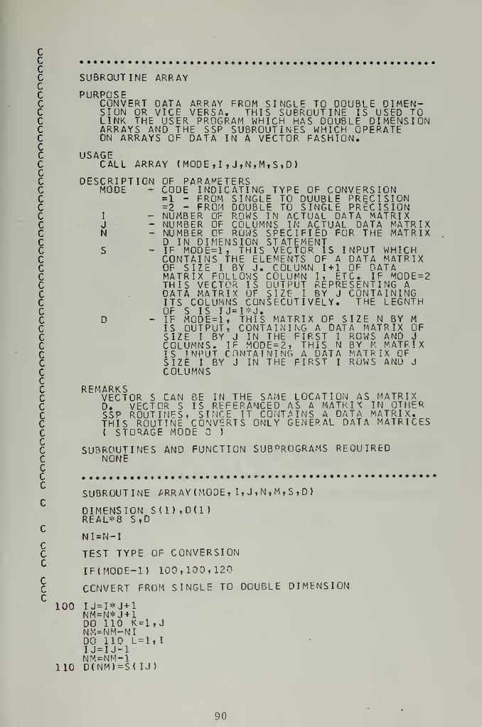
cc ,
cC SUBROUTINE ARRAYCC PURPOSEC CONVERT DATA ARRAY FROM SINGLE TO DOUBLE DIMEN-C SION OR VICE VERSA. THIS SUBROUTINE IS USED TOC LINK THE USER PROGRAM WHICH HAS DOUBLE DIMENSIONC ARRAYS AND THE SSP SUBROUTINES WHICH OPERATEC ON ARRAYS OF DATA IN A VECTOR FASHION.CC USAGEC CALL ARRAY ( MODE , I , J , N, M, S , D
)
CC DESCRIPTION OF PARAMETERSC MODE - CODE INDICATING TYPE OF CONVERSIONC =1 - FROM SINGLE TO DUUBLE PRECISIONC =2 - FROM DOUBLE TO SINGLE PRECISIONC I - NUMBER OF ROWS IN ACTUAL DATA MATRIXC J NUMBER OF COLUMNS IN ACTUAL DATA MATRIXC N NUMBER OF ROWS SPECIFIED FOR THE MATRIXC D IN DIMENSION STATEMENTC S - IF MODE=l, THIS VECTOR IS INPUT WHICHC CONTAINS THE ELEMENTS OF A DATA MATRIXC OF SIZE I BY J. COLUMN 1+1 OF DATAC MATRIX FOLLOWS COLUMN I t ETC. IF MODE=2C THIS VECTOR IS OUTPUT REPRESENTING AC DATA MATRIX OF SIZE I BY J CONTAININGC ITS COLUMNS CONSECUTIVELY. THE LEGNTHC OF S IS IJ=I*J.C D - IF MODE=l, THIS MATRIX OF SIZE N BY MC IS OUTPUT, CONTAINING A DATA MATRIX OFC SIZE I BY J IN THE FIRST I ROWS AND J
C COLUMNS. IF MODE=2, THIS N BY M MATRIXC IS INPUT CONTAINING A DATA MATRIX OFC SIZE I BY J IN THE FIRST I RUWS AND J
C COLUMNSCC REMARKSC VECTOR S CAN BE IN THE SAME LOCATION AS MATRIXC D. VECTOR S IS REFERANCED AS A MATRIX IN OTHERC SSP ROUTINES, SINCE IT CONTAINS A DATA MATRIX.C THIS ROUTINE CONVERTS ONLY GENERAL DATA MATRICESC ( STORAGE MODE )
C SUBROUTINES AND FUNCTION SUBPROGRAMS REQUIREDC NONECc
SUBROUTINE ARRAY(MODE T I,J,N,M,S,D)C
DIMENSION S(l) ,D(1
)
REAL*8 StDC
NI-N-1r
C TEST TYPE OF CONVERSIONC
CCC
IF(MODE-l) 100,100,120
CONVERT FROM SINGLE TO DOUBLE DIMENSION
100 IJ=I*J+1NM=N*J+1DO 110 K=1,JNM=NM-NIDO 110 L = l, I
IJ=IJ-1NM=NM-1
110 D(NM)=S(IJ)
90

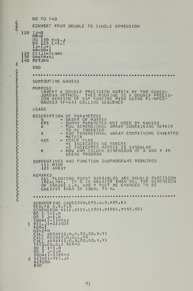
GO TO 140CC CONVERT FROM DOUBLE TO SINGLE DIMENSION
120 IJ=0NM=0DO 130 K =1,JDO 125 L = 1,I1J=IJ+1NM=NM+1
125 S( IJ)=D(NM)130 NM=NM+NI140 RETURN
CEND
CccC SUBROUTINE GAUSS3CC PURPOSEC INVERT A DOUBLE PRECISION MATRIX BY THE GAUSS-C JORDAN METHOD. THIS ROUTINE IS A DOUBLE PRECIS-C ION VERSION OF SSP ROUTINE MINV USING Fl-NPGS-C GAUSS3 (F-63) CALLING SEQUENCECC USAGECC DESCRIPTION OF PARAMETERSC N ORDER OF MATRIXC EPS - DUMMY PARAMETER NOT USED BY GAUSS3C A TWO DIMENSIONAL ARRAY CONTAINING MATRIXC TO BE INVERTEDC X TWO DIMENSIONAL ARRAY CONTAINING INVERTEDC MATRIXC KER - ERROR FLAGC =1 INDICATES NO ERRORSC =2 INDICATES MATRIX IS SINGULARC K ROW AND CCLUMN DIMENSION OF A AND X INC USERS PROGRAMCC SUBROUTINES AND FUNCTION SUBPROGRAMS REQUIREDC (1) MINVC (2) ARRAYCC REMARKSC ALL FLOATING POINT VARIABLES ARE DOUBLE PRECISIONC (RFAL*8). IF N IS GREATER THAN 50, THE DIMENSIONC OF ARRAYS L,M, AND Y MUST BE CHANGED TO BEC GREATER THAN OR EQUAL TO N.Ccc
SUBROUTINE GAUSS3 ( N t EPS , A, X, KER , K
)
DIMENSION M i) ,X<1) ,L(50) ,M(50) ,Y(50,5C)DO 1 1 = 1, NDO 1 J=1,NIND=( I-1)*K+J
1 Yd, J) = A(IND)KER=1N2=2*NCALL ARRAY(2,N,N,5O,50,Y,Y)CALL MINV(Y,N,D,L,M)CALL APRAY( 1,N,N, 50,50, Y,Y)IFtD.EQ.O.) KER=2DO 2 I=1,NDO 2 J=1,NIND=( 1-1 )*K+J
2 X( IND)=Y( I, J)RETURNEND
91


cc ,
cC SUBROUTINE MINVCC PURPOSEC INVERT A DOUBLE PRECISION MATRIX BY THE GAUSS-C JORDAN METHOD.CC USAGEC CALL MINV(A,N,D,L,M)CC DESCRIPTION OF PARAMETERSC A INPUT MATRIX, DESTRGYED IN COMPUTATIONC AND REPLACED BY RESULTANT INVERSE.C N ORDER OF MATRIX AC D RESULTANT DETERMINANTC L - WORK VECTOR OF LEGNTH NC M - WORK VECTOR OF LEGNTH NCC SUBROUTINES AND FUNCTION SUBPROGRAMS REQUIREDC NONECC REMARKSC NONECCc
SUBROUTINE MI NV ( A, N , D, L , M
)
DIMENSION A(l) ,L(1) ,M( 1)DOUBLE PRECISION A , D ,B I GA, HOLD
CC SEARCH FOR LARGEST ELEMENTC
D = 1.0
DO 80 K = 1,NNK=NK+NL(K)=KM(K)=KKK=NK+KBIGA=A(KK)DO 20 J = K
TN
IZ=N*( J*l)D0_20 I=K,N
10 IF(DABS(BIGA)-DABS( A(IJ) ) ) 15,20,2015 BIGA=A( IJ)
L(K)=IM(K)=J
20 CONTINUECC INTERCHANGE ROWSC
J=L(K)IF(J-K) 35,35,25
25 KI=K-NDO 30 1=1,
N
KI=KI+NHOLD=-A(KI
)
JI=KI-K+JA(KI)=A( JI
)
30 AUI) =HOLD
C INTERCHANGE COLUMNSC
35 I=M(K) r ^ nIF(I-K) 45,45,38
38 JP=N*(I-1)DO 40 J=1,NJK=NK+JJI=JP+J
92

HOLD=-A( JK)A( JK)=A( JI
)
40 A(JI) =H0LDCC « DIVIDE COLUMN BY MINUS PIVOT (VALUE OF PIVOTC ELEMENT IS CONTAINED IN BIGA)C
45 IF(BIGA) 48,46,4846 D=0.0
RETURN48 DO 55 1=1,
N
IF(I-K) 50,55,5050 IK=NK+I
A(IK)=A( IK)/(-BIGA)55 CONTINUE
CC REDUCE MATRIXC
DO 65 1=1,
N
IK=NK+IHOLD=A( IK)IJ=I-NDO 65 J=1,NIJ=IJ+NIF(I-K) 60,65,60
60 IF(J-K) 62,65,6262 KJ=IJ-I+K
A( IJ)=HOLD*A(KJ )+A( IJ)65 CONTINUE
CC DIVIDE ROW BY PIVOTC
KJ=K-NDO 7 5 J=1,NKJ=KJ+NIF(J-K) 70 T 7^,70
70 A(KJ)=A(KJ l/BIGA75 CONTINUE
D=D*BIGACC REPLACE PIVOT BY RECIPROCALC
A(KK)=1.0/3IGA80 CONTINUE
C FINAL ROW AND COLUMN INTERCHANGEC
K=N100 K=(K-1)
IF(K) 150,150,105105 I=L(K)
IF(I-K) 120,120,108108 JC=N*(K-1)
JR=N*( 1-1)DO 110 J=1,NJK=JQ+JHOLD=A( JK)JI=JR+JA(JK)=-A( JI
)
110 A(JI) =HOLD120 J=M(K)
IF(J-K) 100,100,125125 KI=K-N
DO 130 1=1 tNK1=KI+NH0LD=A(KI)JI=KI-K+JA(KIJ=-A(JI )
130 A(JI) =HCLOGO TO ICC
150 RETURNEND
93


cccC SUBROUTINE PRODCC PURPOSEC TO COMPUTE THE PRODUCT OF TWO MATRICESCC USAGEC CALL PROD(A,B,C,N,M,L)CC DESCRIPTION OF PARAMETERSC A - FIRST INPUT MATRIXC B - SECOND INPUT MATRIXC C PRODUCT OF A AND BC N NUMBER OF ROWS IN A AND CC M NUMBER OF COLUMNS IN A AND ROWS IN BC L NUMBER OF COLUMNS IN B AND CCC REMARKSC NONECC SUBROUTINES AND FUNCTION SUBPROGRAMS REQUIREDC NONECcc
SUBROUTINE PROD ( A, B , C, N, M, L
)
REAL*8 A(9,9) ,B(9,9) ,C(9,9)DO 1 1=1 »NDO 1 J-1,LC(I, J)=0.00DO 1 K=1,M
1 C( I
,
J)=C(I ,J)+A( I,K)*B(K, J)RETURNEND
Cccc ,
cC SUBROUTINE SUMMCC PURPOSEC ADD TWO MATRICESCC USAGEC CALL SUMM(A,B,C T M,N)CC DESCRIPTION OF PARAMETERSC A NAME OF FIRST INPUT MATRIXC B NAME OF SECOND INPUT MATRIXC C NAME OF OUTPUT MATRIXC M NUMBER OF ROWS IN A,B, AND CC N NUMBER OF COLUMNS IN A,B, AND CCC REMARKSC NONECC SUBROUTINES AND FUNCTION SUBPROGRAMS REQUIREDC NONECcc
SUBROUTINE SUMM( A , B t C » M, N)REAL*8 A(9,9) ,B(9,9),C(9,9)DO 1 1=1,
M
DO 1 J=1,N1 C(I, J)=A(I, J)+B( I, J)
RETURNEND
94

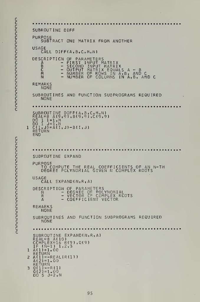
cccC SUBROUTINE DIFFCC PURPOSEC SUBTRACT ONE MATRIX FROM ANOTHERCC USAGEC CALL DIFF(A f B,Cf M,N)CC DESCRIPTION OF PARAMETERSC A FIRST INPUT MATRIXC B SECOND INPUT MATRIXC C OUTPUT MATRIX EQUALS A - BC M NUMBER OF ROWS IN A T B, AND CC N NUMBER OF COLUMNS IN A»B, AND CCC REMARKSC NONECC SUBROUTINES AND FUNCTION SUBPROGRAMS REQUIREDC NONECcc
SUBROUTINE DIF F ( A, B , Ct M,N )
REAL*8 A(9 f 9) , B(9,9J ,0(9,9)DO 1 1=1,
M
DO 1 J=1,N1 C( It J)=A( I, J)-B( I, J)
RETURNEND
Cccc • ,
cC SUBROUTINE EXPANDCC PURPOSEC TO COMPUTE THE REAL COEFFICIENTS OF AN N-THC DEGREE POLYNOMIAL GIVEN N COMPLEX ROOTSCC USAGEC CALL EXPAND(N,R, A)CC DESCRIPTION OF PARAMETERSC N DEGREE OF POLYNOMIALC R VECTOR C(= COMPLEX ROOTSC A COEFFICIENT VECTORCC REMARKSC NONECC SUBROUTINES AND FUNCTION SUBPROGRAMS REQUIREDC NONECCc
SUBROUTINE EXPAND(
N
T R» A
)
REAL*8 A(10)CCMPLEX*16 R(9 ) ,Q(9)IF (N-l) 1,2»3A(l)=1.00RETURNA(1)=-REAL(R(1 )
)
A(2)=1.00RETURNQ(l)=-R(l)Q(2)=1.00DO 5 J=2,N
95


Q(J+1)=1.00JJ=J-1DO 4 I=1»JJK = J-I
4 Q(K+1)=Q(K)-Q(K+1)*R(J)5 Q(1)=-Q(1)*R(J)6 N1=N+1
DO 7 L=1,N17 A(U=REAL(Q(L) )
RETURNEND
96

BIBLIOGRAPHY
1. Nieman, R. E., Fisher, D. G., and Seborg, D. E "AReview of Process Identification and Parameter Es-timation Techniques," Internation al Journal ofControl, V. 13, No. 2, p. 209-26 4, May 1971.
2. Eykhoff, P., van der Grinten, M. , Kwakernaai, H.and Veltman, B., "Survey-Systems Modeling and Iden-t
1?^?
n,n Third Congress of I.F.A.C. . London,June 1966. " "
3. Mishkin E., and Haddad, R. A., "Identification andCommand Problems in Adaptive Systems," IRE Transon Automatic Control , V. AC-4, No. 2, p . 121-131
*
November 1959. '
4. Levin M. J., "Optimum Estimation of Impulse Responsein the Presence of Noise," IRE Trans, on CircuitTheory, V. CT-7, No. 1, p. 50-56, March 1960.
5. Kerr, R. B., and Surber, Jr., N. H., "Precision ofImpulse Response Identification Based on ShortNormal Operating Records," IRE Trans, on AutomaticCjjntrol, V. AC-6, No. 2, p. "173-182, May 1961.
6. Turin, G. L., "On the Estimation in the Presence ofNoise of the Impulse Response of a Random, LinearFilter," IRE Trans, on Information Theory, V IT-3No. 1, p. 5-10, March 1957.
~^~
7. Lichtenberger, W. W. , "On the Identification of Lin-ear Processes," IRE Trans, on Circui t Theory, V CT-7No. 1, p. 7 8-79, March 1960.
8. Lichtenberger, W. W., "A Technique of Linear SystemIdentification Using Correlating Filters," IRE Trans .
on Automatic Control , V. AC- 9, No. 2, p. lST^!)May 1961.
9. Hill, J. D., and McMurtry, "An Application of DigitalComputers to Linear System Identification," IEEETrans, on Automatic Control , V. AC-9, No. 5, p. 536-538, October 1964.
10. Lindenlaub, J. C, and Cooper, G. R. , "Noise Limita-tions of System Identification Techniques," IEEETrans, on Automatic Control , V. AC -10, No. 1 , p. 4 3-48, January 1963.
97

12. Nagumo J and Noda, A., "A Learning Method for Sys-
V A? ?5 M1Ca
T10n
'"oFE TranS'
°n Automatic Control,V. AC-12, No. 3, p. 282-287, June 1967.
13. Bass, R Testing Function Techniques i n System Iden-tification,Ph.D. Disse rlaLion, University ofCalifornia, Berkeley, March 1969.
14. Astrom, K J., and Bohlin, T. , "Numerical Identifica-tion of Linear Dynamic Systems from Normal Operating*ec °rds•
" IFAC Symposium - Theory of Self -Adapt ive§
Systems, Teddington, 1965. *
15. Peterka, V., "New Approach to the Identification of
1968r6te DynamiC S >' stems >" Kybernetika
, V. 4, No. 5,
16. Peterka, V and Smuk , K., "On-Line Estimation ofDynamic Model Parameters from Input-Output Data "IFAC Congress . Warsaw, 1969.
17. Ho, B. L., and Kalman, R. E., "Effective Constructionof Linear State Variable Models from Input/OutputFunctions," Sonderdruck aus Re gelungstechni k V 14No. 12, p. 545-548, 1966. '
'
18. Eldem, I., Identification of Plant Dynamics Using Ho '
s
Algorithm, MS Thesis, United States' Naval PostgraduateSchool, Monterey, California, 1969.
19. Shinbrot, M. , "On the Analysis of Linear and NonlinearSystems," Trans, of the ASME , V. 79, No. 3 p 547-552April 1957.
' '
20. Mowery, V. 0., "Least Squares Recursive Differential-Correlation Estimation in Nonlinear Problems," IEEETrans
.on Automatic Control, V. AC-10, No 4* p 599-
407, October 1965.P '
21. Fairman, F. W. , Process Parameter Estimation bv theMoment Function Method , Ph.D. Dissertation, Universityof Pennsylvania, 1968.
22. Bellman, R. E., Kagiwada, H., and Kalaba, R. E.,"Quasi-Linearization, System Identification and Pre-diction," Rand Corp. Report RM-5821-PR , August 1963.
98


23. Hsieh, H. C, "Adaptive Control Systems," Advances inControl Systems , V. 2, Academic Press Inc. , New York,New York, 1965.
24. Simpson, H. R. , "A Sampled Data Nonlinear Filer," Proc .
of the IEEE , V. 112, No. 6, p. 1187-1196, June 1965.
25. Bose, A. G., "A Theory for the Experimental Determina-tion of Optimum Nonlinear Systems," IRE NationalConvention Record , Part 4, p. 21-30, 1956.
26. Bose, A. G., "Nonlinear System Characterization andOptimization," IRE Trans, on Circuit Theory , SpecialSupplement, p. 30-40, 1959.
27. Hubbell, P. C, Digital Identification and Simulationof Nonlinear Systems with Physiological Applications ,
Ph .D . Dissertation, University of Pennsylvania,Philadelphia, Pennsylvania, 1967.
28. Diamessis, J. E., "A New Mthod for Determining theParameters of Physical Systems, Proc. of the IEEE
,
V. 53, No. 2, p. 205-206, February 1965.
29. Diamessis, J. E., "On the Determination of the Param-eters of Physical Systems," Proc. of the IEEE , V. 53,No. 3, p. 319-320, iMarch 196 5.
30. Wang, P. P., "On the Evaluation of the Parameters ofa Nonlinear System," Proc. of the IEEE , V. 55, No. 3,
p. 468-469, March 1967.
31. Golub, G., "Numerical Methods for Solving Linear LeastSquares Problems," Numerische Mathematik, V. 7, p.
206-216, 1965.
32. Businger, P., and Golub, G., "Linear Least SquaresSolutions by Householder Transformations," NumerischeMathematik, V. 7, p. 269-276, 1965.
99

INITIAL DISTRIBUTION LIST
No. Copies
1. Defense Documentation CenterCameron StationAlexandria, Virginia 22314
2. Library, Code 0212Naval Postgraduate SchoolMonterey, California 93940
3. Professor George J. Thaler, Code 52TrDepartment of Electrical EngineeringNaval Postgraduate SchoolMonterey, California 93940
4. Mr. Joseph Rub isNaval Ships Research § Development CenterAnnapolis, Maryland 21402
5. Mr. Hal StephensInternational Business MachinesBui l/linn ni/iUlxUljlg <J J. T
Monterey $ Cottle RoadsSan Jose, California 95114
6. Doctor Ken DeckertInternational Business MachinesMonterey $ Cottle RoadsSan Jose, California 95114
7. ENS William R. Hansell USN44 Ann RoadBroomall, Pennsylvania 19008
100


UNCLASSIFIEDSecurity Classification
DOCUMENT CONTROL DATA -R&DiSecurtty classification of title, body of abstract and indexing annotation must be entered when the overall report (s classified)
Originating activity (Corporate author)
Naval Postgraduate SchoolMonterey, California 93940
21. REPOST SECURITY CLASSIFICATION
UNCLASSIFIED2b. GROUP
3 REPO R T TITLE
IDENTIFICATION OF SYSTEM DYNAMICS USING MULTIPLE INTEGRATIONS
4 DESCRIPTIVE NOTES (Type of report and, inclusive dates)
Master's Thesis; June 1971S auTmORiS) (First name, middle initial, last name)
William R. Hansell
6 REPOR T D A TE
June 19717«. TOTAL NO. OF PAGES
1027b. NO. OF REFS
32• a. CONTRACT OR GRANT NO
b. PROJEC T NO
9a. ORIGINATOR'S REPORT NUM6ERIS)
9b. OTHER REPORT NOtS) (Any other number* that may be atal^nedthis report)
10 DISTRIBUTION STATEMENT
Approved for public release; distribution unlimited
11. SUPPLEMENTARY NOTES 12. SPONSORING MILITARY ACTIVITY
Naval Postgraduate SchoolMonterey, California 93940
13 ABSTRACT
A practical methovariant systems on therecords is reviewed an
the system is not initis implemented using a
of a numerical integrasolving overdeterminedSeveral examples are pand present capabiliti
d for identifying linear time in-
basis of arbitrary input-outputd extended to handle the case whereially in the zero state. The methoddigital computer program composedtion subroutine and a subroutine for
sets of linear algebraic equations.resented to demonstrate the accuracyes of the procedure.
DD FORMi nov es
S/N 0)01 -807-681 1
1473 (PAGE 1
)
UNCLASSIFIED101 Security Classification
A-3140S

UNCLASSIFIEDSecurity Classification
KEY WO R OS
Linear Systems
Identification
Multiple Integrals
Modeling
)D .
F.T.,1473
/N 01 Ot -807-632 1
BACK) IINCT.ASSTFTED
102Security Classification 3 1403


ThesisH1995c.l
Thesi s
H1995c.l
129105Hansel 1
Identification of
system dynamics using
multiple integrations.
21 JAN as 3 3293
129105Hansel 1
Identi f ication of
system dynamics usingmultiple integrations.

thesH1995
Identification of system dynamics using
3 2768 001 01775 9
DUDLEY KNOX LIBRARY