DIPARTIMENTO DI SCIENZE ECONOMICHE AZIENDALI E STATISTICHE

Via Conservatorio 7 20122 Milano

tel. ++39 02 503 21501 (21522) - fax ++39 02 503 21450 (21505) http://www.economia.unimi.it

E Mail: dipeco@unimi.it

IDENTIFICATION IN STRUCTURAL VAR MODELS WITH DIFFERENT

VOLATILITY REGIMES

EMANUELE BACCHIOCCHI

Working Paper n. 2011-39

DICEMBRE 2011

Identification in Structural VAR models with different volatility

regimes

Emanuele Bacchiocchi∗

14th December 2011

Abstract

In this paper we study the identification conditions in structural VAR models with differentregimes of volatility. We propose a new specification that allows to address identification in theconventional likelihood-based setup. A formal general framework for identification is developpedand it is proved that exact-identification assumptions in the standard SVAR literature appearhere to be over-identified, and thus subject to statistical inference. The empirical relevance of themethodology is discussed through an empirical application concerning the relationships betweenterm structure of interest rates and output growth.

Keywords: SVAR, heteroskedasticity, identification.JEL codes: C01,C13,C30,C51.

I Introduction

In the Structural Vector Autoregression (SVAR) literature the problem of identification refers to thedefinition of instantaneous correlations among independent shocks that are otherwise hidden in thecovariance matrix of the VAR innovations. Since the seminal work by Sims (1980), many approacheshave been proposed, regarding triangularization of the correlation matrices (Amisano and Giannini,1997), long-run constraints (Blanchard and Quah, 1989; King et al., 1991; Pagan and Pesaran,2008),identification of only a subset of all the shocks (Christiano et al., 1999), inequality constraints (Uhlig,2005; Canova and De Nicolo, 2002; Faust, 1998), Bayesian techniques (Koop, 1992). Rubio-Ramirezet al. (2010) have recently proposed a very general framework that allows to check for the globalidentification of structural VAR models with linear and certain nonlinear restrictions on the param-eters. The authors establish an easily implementable rank condition which is sufficient for generalidentification and necessary and sufficient for exact identification.

In the last years, the literature has benefitted from the idea that heteroskedasticity or otherpeculiarities in the data can add important information to the identification of simultaneous equationssystems (Rigobon, 2003; Klein and Vella, 2003; Lewbel, 2011). In this direction, Lanne and Lutkepohl(2010) use the distributional features of the residuals to identify structural shocks, while Lanne andLutkepohl (2008) and Lanne et al. (2010) discuss identification of the structural parameters of the

∗Department of Economics, University of Milan. Email emanuele.bacchiocchi@unimi.it

1

SVAR models in the presence of different regimes of volatility. Our paper moves in this directionand provides a formal general framework that allows us to study identification as in the conventionallikelihood-based approach in the spirit of Rothenberg (1971). Morevere, as done by Johansen (1995)in the context of linear models, and Lucchetti (2006) for general covariance structures, in the presentpapar we discuss necessary and sufficient conditions for identification that do not depend on theestimated parameters, but on the combination of imposed constraints and the kind of heteroskedastictycharacterizing the model.

The model developped in the paper is based on the assumptions that the different regimes ofvolatility are known and that such regimes do not alter the structural parameters of the SVAR.The only effects of volatility states are thus confined to the covariance matrices of the reduced forminnovations. Such assumptions are common with those of Lanne and Lutkepohl (2008) and Lanne etal. (2010), but in our specification we allow the covariance matrices to vary among states in a reacherway than simple multiplicative factors regarding the variances only. As a consequence, the impulseresponse functions vary across the different regimes of volatility. Rubio-Ramirez et al. (2005) and Simsand Zha (2006) also consider SVAR models with different regimes of volatility and different impulseresponses, although in their specifications, based on Markov regime switching, all the parameters ofthe SVAR are allowed to vary across regimes.

The particular specification of the model gives us the possibility of formally studying the identifi-cation of the structural parameters even in the case the heteroskedasticity involves a reduced numberof variables. This allows to check for identification without the need to separate the analsys intosubsystems of homoskedastic and heteroskedastic dependent variables, as instead done in Lanne andLuktepohl (2008).

Given the particular specification of the heteroskedastic SVAR model, the general rank conditionproposed by Rubio-Ramirez et al. (2010) reveals to be not implementable. For this reason, we proposethree alternative strategies for studying the identification of the parameters. The first one refers tothe seminal contribution by Rothenberg (1971) and focus on the rank of the Jacobian matrix. Thesecond and third, instead, concentrate on the uniqueness of the parameter matrices among the class ofall possible admissible ones. In particular, followint the idea of Johansen (1996) and Lucchetti (2006),we provide an easily implementable necessary and sufficient condition for identification that is only afunction of the restrictions imposed on the parameters and the characteristics of the different regimesof volatility.

Our heteroskedastic SVAR model, and the related identification analysis, is shown to be generalenough to replicate and generalize alternative models already discussed in the literature.

The empirical relavance of the theoretical framework developpend in the paper is discussed throughan application which relates to the interconnections between the term structure of interest rates andthe growth rate of the GDP. The evidence on different regimes of volatility provided by the ‘GreatModeration’ literature offers an important source of information that could be used in the analysis ofthe predictive power of the yield curve in forecasting output growth. We thus complement the dynamicmodel for GDP growth and yields developped by Ang et al. (2006) with the possible heteroskedasticityobserved in the data. The results support the idea that both the relations and the predictive powerof the yield curve on GDP growth changes during the pre- and post-Volcker periods.

The rest of the paper is organized as follows: In Section II we present the specification of the modelwhile conditions for identification of the structural parameters are discussed in Section III. Section IVand Section V relates our model to the traditional SVAR specifications, both for homoskedastic andheteroskedastic structural shocks. Section VI presents a FIML estimator for the heterskedastic SVARmodel and discusses some basic inferential aspects. Section VII proposes an empirical applicationwhile Section VIII provides some concluding remarks.

2

II A SVAR model with different regimes of volatility

The model is based on a variation of the AB-specification proposed by Amisano and Giannini (1997)in which, however, we include the possibility of different levels of heteroskedasticity in the data. Letthe data generating process follows a VAR model of the form

yt = A1yt−1 + · · ·+Apyt−p + ut (1)

where yt is a g-dimensional vector of observable variables, and ut a vector of innovations with non-constant covariance matrix, i.e. ut ∼ L (0,Σt). The covariance matrix Σt hiddens all possible si-multaneous relationships among uncorrelated structural shocks εt ∼ (0, Ig), and can be defined asΣt = A−1CtC

′tA′−1, where A and Ct are the structural parameters that connects the reduced form

innovation ut with the uncorrelated shocks εt in the following way:

Aut = Ctεt. (2)

The matrix Ct accounts for possible heteroskedasticity and is defined as follows

Ct = (Ig +BDt) (3)

where the matrix Dt is a diagonal matrix assuming only 0 − 1 values, indicating whether, at time t,the i-th endogenous variable is in a state of high (1) or low (0) volatility. The heteroskedasticity, thus,is intended as different regimes of volatility that might apply to one or more variables in the system.When all variables are in a state of low volatility (Dt = 0), the model in (2) reduces to the K-model inthe terminology of Amisano and Giannini (1997), while when one or more variables are in a state ofhigh volatility the correlation structure becomes more complicated and involves both interdependencesamong variables and among structural shocks1. In the state of low volatility the correlations amongthe endogenous variables are captured by the A matrix as in the traditional systems of equations butwith two important improvements: a) less stringent constraints for obtaining identification, as provedin the next section; b) the error terms are uncorrelated and can be interpreted as structural shocks asin the conventional SVAR literature.

Differently with respect to Lanne and Luktepohl (2008), we do not impose any form of triangular-ization in the A matrix for obtaining identification. Moreover, the transmission of structural shocksin states of high volatility, captured by the combination of B and Dt, might be different among thestates. When a structural shock hits the economy, depending on the particular regime of volatility,it propagates differently among all the other variables of the system. While in Lanne and Lutkepohl(2008) and Lanne et al. (2010) the differences among the states are confined to different variancesof the structural shocks, in the present specification we allow for differences in the covariances too.The consequences for the identification of the parameters are not trivial and are analyzed in the nextsection.

Suppose the SVAR model defined in (1)-(3) is enriched with the distributional assumption that

ut ∼ N (0,Σt) (4)

where,Σt = A−1CtC

′tA′−1 (5)

represents the covariance matrix in the different states of volatility, as a function of the structuralparameters A and, indirectly, B . All the information concerning Σt is contained in the residuals ofthe VAR model ut and in the Dt matrices indicating the states of volatility.

1A similar specification has been proposed by Favero and Giavazzi (2002) in which, however, Dt refers to simpleintervention dummies, and the identification problem has been solved with exclusion restrictions in the dynamic part ofthe model.

3

The log-likelihood function for the parameters of interest is

L (A,B) = c+T

2log |A|2 − 1

2

T∑t=1

log |Ct|2 −12

T∑t=1

tr(A′C−1′

t C−1t Autu

′t

). (6)

The log-likelihood function can also be written in a more compact form as

L (A,B) = c+T ∗

2log |(Is ⊗A)|2 − T ∗

2log |B∗|2 − 1

2tr[T ∗(Is ⊗A′

)B∗−1′B∗−1 (Is ⊗A) Σ

](7)

where s indicates the number of distinct states of volatility and the (gs× gs) matrix B∗ is defined as

B∗ = (Igs + (Is ⊗B)D) (8)

where D is a block diagonal matrix of the form

D =

D1

. . .Ds

(9)

where Di is the diagonal (g × g) matrix describing the i-th state of volatility. More precisely, asdescribed before, it presents Dijj = 1 whether the j-th endogenous variable is in a state of highvolatility and 0 if it is in a state of low volatility. Σ is the (gs× gs) block diagonal matrix that collectsthe estimates of the covariance matrices in each state

Σ =

Σ1

. . .Σs

(10)

where Σi = 1/Ti∑Ti

t=1 utu′t, for i = 1 . . . s. In the same way we can define the corresponding theoretical

second moments for the error terms as:

Σ =

Σ1

. . .Σs

. (11)

The matrix T ∗ is defined as

T ∗ = (Ig ⊗ T ∗∗) with T ∗∗ =

T1

. . .Ts

(12)

and indicates the number of elements in the sample for each state of volatility. This new parameteri-zation reveals to be extremely useful for investigating the order and rank conditions for identificationas reported in the following sections. As a first consequence, using this new parameterization, therelation connecting the parameters of the strucural and reduced form in Eq. (5) can be rewritten as

(Is ⊗A) Σ(Is ⊗A′

)= [Igs + (Is ⊗B)D] [Igs + (Is ⊗B)D]′ , (13)

that considers all the information contained in the different states of volatility without explicitlyconsidering the dependence with respect to t. This new formulation will be largely used in the nextsections discussing the identification criteria for the structural parameters A and B.

Throughout, use is made of the following notation: Kgs is the g2s2 × g2s2 commutation matrixas defined in Magnus and Neudecker (2007), Ngs = 1/2 (Igs +Kgs), while the F matrix2 is suchthat, given two matrices A (m× n) and B (p× q), then vec (A⊗B) = (F ⊗ Ip) vecB, where F =(In ⊗Kqm) (vecA⊗ Iq).

2This matrix corresponds to the H matrix defined in Magnus and Neudeckers (2007) pag. 56.

4

III Identification

In the general AB-model proposed by Amisano and Giannini (1997) the problem of identification ofthe structural parameters arises because, if we define two new matrices

A1 = QA and B1 = QBH (14)

with Q invertible and H orthogonal, then the standard relation among the parameters of the reducedand structural forms AΣA′ = BB′ becomes

A1ΣA′1 = B1B′1 ⇒ QAΣA′Q′ = QBHH ′B′Q′

⇒ Σ = A−1Q−1QBHH ′B′Q′Q−1′A−1′

⇒ Σ = A−1BB′A−1′,

indicating that the matrices A1 and B1 can be considered an alternative reparemetrization of theoriginal model3. The traditional approach to reach identification consists in imposing q = qA + qBlinear constraints on the parameters as follows

RAvecA = rA

RBvecB = rB (15)

or, in the usual explicit form

vecA = SAθA + sA

vecB = SBθB + sB (16)

where θ = (θ′A, θ′B)′ represents the vector of unconstrained parameters. Amisano and Giannini (1997)

find the conditions for local identification for the AB-model in the standard likelihood approach pro-posed by Rothenberg (1971). In the next section we follow the same strategy and discuss the necessaryand sufficient conditions for local identification in the SVAR model with heteroskedasticity presentedin Section II.

Henceforth, we shall use interchangeably both the implicit- (Eq. (15)) and explicit-form (Eq. (16))representation of the identification constraints. Moreover, for future use we introduce the followingdefinitions:

Definition 1 [Admissible matrix] A matrix of parameters is said to be admissible when it satisfiesthe linear restrictions as in Eq. (15) or, equivalently, in Eq. (16).

Definition 2 [Infinitesimal rotation] Given a vector x0, an infinitesimal transformation4 is definedas x1 = (I +H)x0 where the matrix H is infinitesimal and I is the identity matrix. Theparticular infinitesimal rotation case requires the matrix H to be orthogonal. An interestingproperty is that H is hemisymmetric, i.e. H = −H ′.

3Rubio-Ramirez et al. (2010) proposed sufficient rank conditions for the global identification when linear and certainnonlinear constraints are imposed on the parameters. Their specification of the SVAR model is of the form

A0yt = A1yt−1 + . . .+Apyt−p + εt

and does not admit the possibility of simultaneous relationships among both the endogenous variables and the structuralshocks, as instead it happens for the AB-model used in this paper. Their sufficient rank condition, thus, cannot beapplied to our model.

4See Weisstein (2004) for a detailed treatment of the infinitesimal rotation operator.

5

III.1 Identification I: The Jacobian matrix

In this section we study the identification of the strucutral parameters based on the traditional ap-proach proposed by Rothenberg (1971). The following proposition provides the sufficient condition forlocal identification for the structural parameters of SVAR models with different regimes of volatilitydefined in Eqs. (1)-(3).

Proposition 1 Suppose the DGP follows a VAR model as defined by Eqs. (1)-(4) with s ≥ 2 differentstates of volatility as assumed in Eq. (11). Assume further that prior information is available in theform of q linear restrictions on A and B as in Eq. (15). Then (A0, B0) are locally identified if andonly if the matrix

J (A0, B0) =

−2NgsE1 (HA ⊗ Ig) 2NgsE2 (HB ⊗ Ig)RA 00 RB

(17)

has full column rank 2g2, where

E1 =[(Is ⊗A)−1B∗B∗′

(Is ⊗A′

)−1 ⊗ (Is ⊗A)−1]

(18)

E2 =[(Is ⊗A)−1B∗D ⊗ (Is ⊗A)−1

](19)

with B∗ and D defined as in Eq. (8) and Eq. (9), respectively.

Proof : Appendix A.

The general framework proposed by Rothenberg (1971) for the identification of parametric modelsrefers to the system of homogeneous equations relating the parameters of the structural form (uniden-tified), with those of the reduced form (identified). When the unique solution for such a system isrepresented by the null vector, then the parameters of the structural form are identified.

The idea of Proposition 1 follows this intuitive strategy while the technical details for provingthe result are discussed in the appendix. As expected, the condition for local identification of thestructural parameters depends on the particular form of heteroskedasticity defined by the D matrix.Although conditions for local identification of heteroskedastic structural models have been alreadydiscussed in the literature, the novelty of this paper is that we combine the information coming fromthe economic theory (the restrictions on A and B) with some important features observed in the data(the heteroskedasticity).

The following corollary, however, shows that when there are s ≥ 2 regimes of volatility it becomespossible to identified the structural parameters of the model even without imposing restrictions on theA matrix.

Corollary 1 Under the assumptions of Proposition 1, the restrictions in RA are not necessary forlocal identification.

Proof : Appendix A.

This corollary provides a generalization of the result in Rigobon (2003), Proposition 1, in whichthe author provides a sufficient condition for identification only for bivariate systems of equations,while the result in our Corollary 1 overcomes this limitation.

Lanne and Lutkepohl (2008) also provide a generalization of the Rigobon’s result. Their approach,as it will be discussed in one of the examples presented in Section V, however, is based on a well known

6

result of matrix algebra in which symmetric and positive definite matrices can be simultaneouslydiagonalized by means of common squared matrices and specific diagonal matrices.

Remark 1. The restrictions on the B matrix, instead, depend on the nature of heteroskedasticityas expressed in the D matrix. The rank of D is equivalent to the number of variables in a state ofhigh volatility. As a consequence, E2 is of reduced rank, making more complicated, although notimpossible, that NgsE2 (HB ⊗ Tg) will have full column rank. In this latter case, the inclusion ofrestrictions in the B matrix becomes not necessary for identification.

In the traditional literature on SVAR models, or more generally in simultaneous equations systems,the order condition refers to the system connecting the parameters of the structural form to those ofthe reduced form. Obviously, it is expected that the number of equations to be at least as large asthe number of unknowns. In practice, the number of rows of the Jacobian matrix must be as largeas the number of columns. Without any further alternative strategy, restrictions on the parametersare always necessary for identifing the structural parameters of the model. As an example, in theCholesky-type structuralization of a SVAR model, the order condition is satisfied in that the numberof equations, n (n+ 1) /2, exactly matches the number of free parameters (a number of n (n− 1) /2zero restrictions must be imposed).

Remark 2. In the heteroskedastic SVAR model proposed in this paper, instead, the necessarycondition requiring a number of rows in the J matrix larger than (or at least equat to) the number ofcolumns (without any further constraint on the parameters) applies when g2s2 ≥ 2g2, which is alwaystrue when s ≥ 2. In other words, when it is possible to observe at least two different volatility regimes,imposing restrictions on the parameters seems to be no more necessary to reach identification. Thisnecessary condition, being independent on the number of restrictions imposed on A and B, is toorough to be thought like an order condition as in the traditional SVAR literature. Starting from thisresult, however, in the next section we are going to define a more refined order condition consideringboth the number of restrictions on the parameters and the presence of different volatility regimes.

III.2 Identification II: Alternative Admissible Matrices

Similarly to the AB-model discussed above, for each state of volatility the problem of identificationarises because it is possible to define an invertible matrix Q and a set of s orthogonal matrices Hi,with i = 1, . . . , s, such that

Σ1 = A−1Q−1Q [Ig +BD1]H1H′1

[Ig +D1B

′]Q′Q−1′A−1

... (20)Σs = A−1Q−1Q [Ig +BDs]HsH

′s

[Ig +DsB

′]Q′Q−1′A−1.

Under the mentioned conditions for the Q and Hi matrices, it becomes impossible to discriminatebetween

A and QA

B1 and QB1H, where B1 = (Ig +BD1)...

Bs and QBsH, where Bs = (Ig +BDs) .

7

As a consequence, the parameters in A and Bi, and hence B, cannot be identifiable5. The analysis ofidentification is similar to the one proposed by Lucchetti (2006) for the AB-model, in which, however,all the regimes of volatility are jointly considered. The point, thus, is to study whether it is possible todefine new matrices A1 = A+ dA, B11 = B1 + dB,. . ., B1s = Bs + dB that are admissible. Important,the notion of admissibility preovided in Definition 1 refers to the structural parameteres in A andB, while in the identification analysis we concentrate our attention on A,B1, . . . , Bs. However, beingthe generic matrix Di a selection matrix that appropriately selects the columns of B to be involvedin that particular state of volatility, it is possible to define a mapping from the parameters in Bi tothose in B, for each i = 1, . . . , s. In fact, starting from the definition of the Bi matrix and using therestrictions in its explicit notation, then

vecBi = vec (Ig +BDi)= vec Ig + (Di ⊗ Ig) vecB= vec Ig + (Di ⊗ Ig) [SBθB + sB] (21)

from which we obtain that the restrictions for the Bi matrices can be derived from those imposed toB as

SiB = (Di ⊗ Ig)SBsiB = (Di ⊗ Ig) sB + vec Ig, for i = 1, . . . , s. (22)

The matrix SiB, in coincidence with those variables remaining in a low volatility regime in the i-thstate, selected by the Di matrix, will be characterized by null columns. The new matrix of restrictionsin the i-th state, SiB, is thus composed by the non null columns of the SiB matrix, only. This problem,instead, does not affect the siB vector, which will be simply equal to siB.

The corresponding RiB and riB matrices, of dimension(qBi × g2

)and (qBi × 1) respectively, will

be obviouslly defined such that RiBSiB = 0 and RiBs

iB = riB, with qBi being the number of restrictions

in the Bi matrix.Let consider now the following infinitesimal transformations

A+ dA = (Ig +Q)A (23)B1 + dB1 = (Ig +Q)B1 (Ig +H1) (24)

=Bs + dBs = (Ig +Q)Bs (Ig +Hs) (25)

where (Ig +Q) is nonsingular and the generic (Ig +Hi) is orthogonal. From these relationships itemerges that

A1 = (Ig +Q)A (26)B1i = (Ig +Q)Bi (I +Hi)

′ , for i = 1, . . . , s. (27)

However, being A1 and B1i admissible, they must satisfy RAvecA1 = rA and RiBvecB1i = riB which,after some algebra, implies that

RA (Ig ⊗Q) vecA = 0 (28)RiB (Ig ⊗Q) vecBi +RiB

(H ′i ⊗ Ig

)vecBi = 0, for i = 1, . . . , s (29)

where the quantity vecQBQ′ desappears because both matrices are infinitesimal. Moreover, consid-ering the restrictions in the explicit form described in Eq. (22), the previous relations become

RA (Ig ⊗Q)[SAθ + sA

]= 0 (30)

RiB

[(Ig ⊗Q) + (Hi ⊗ Ig)

][SiBθ + siB

]= 0, for i = 1, . . . , s. (31)

5The identification analysis will be referred to Bi = (Ig +BDi), instead of B, in that, being Ig and Di clearly known,once the former is identified, then the latter will be identified too

8

Focusing on each row of the first factor of Eq. (30), we obtain that

e′jRA (Ig ⊗Q) = (vecRAj)′ (Ig ⊗Q) =

[ (Ig ⊗Q′

)vecRAj

]′= (vecQ)′Kg (RAj ⊗ Ig) (32)

where ej is the j -th column of the identity matrix, the g×g matrix RAj is defined such that vecRAj =R′Aej , and Kg is the commutation matrix as previously defined. Repeating the same analysis for eachaddend of Eq. (31) separately, and remembering that Hi is hemysymmetric (Hi = −H ′i), leads to

e′jRiB (Ig ⊗Q) =

(vecRiBj

)′ (Ig ⊗Q)

= (vecQ)′(RiBj ⊗ Ig

), for i = 1, . . . , s (33)

and

e′jRiB

(H ′i ⊗ Ig

)=

(vecRiBj

)′ (H ′i ⊗ Ig

)= − (vecHi)

′ (Ig ⊗Ri′Bj) , for i = 1, . . . , s (34)

with RiBj defined such that vecRiBj = Ri′Bej .Remembering that H is an infinitesimal rotation then vecH = Dgϕ, where Dg, defined in Magnus

(1988), is a g2×g(g−1)/2 full-column rank matrix such that for any g(g−1)/2-dimensional vector v, itholds Dgv := vec(H), with H a g×g skew-symmetric matrix (H = −H ′). The system of homogeneousequations in Eqs. (30)-(31) can thus be rewritten as

q′Kg (RAj ⊗ Ig)[SAθA + sA

]= 0 for j = 1, . . . , qA

q′Kg

(R1Bj ⊗ Ig

) [S1BθB + s1B

]− ϕ′1Dg

(Ig ⊗R1′

Bj

) [S1BθB + s1B

]= 0 for j = 1, . . . , qB1

...

q′Kg

(RsBj ⊗ Ig

) [SsBθB + ssB

]− ϕ′sDg

(Ig ⊗Rs′Bj

) [SsBθB + ssB

]= 0 for j = 1, . . . , qBs

for any q vector of dimension(g2 × 1

)and any generic ϕi vector of dimension (g (g − 1) /2× 1),

i = 1, . . . , s. In a more compact way, it becomes[q′∣∣∣∣ ϕ′1 ∣∣∣∣ ϕ′2 ∣∣∣∣ · · · ∣∣∣∣ ϕ′s ]T (θ) = [0] (35)

with

T (θ) =

UA (θ) U1

B (θ) U2B (θ) · · · U sB (θ)

−T 1B (θ)

−T 2B (θ)

. . .−T sB (θ)

(36)

where

UA (θ) =[UA1θ + uA1

∣∣∣∣ · · ·∣∣∣∣UAqAθ + uAqA

]for j = 1, . . . , qA and i = 1, . . . , s

U iB (θ) =[U iB1θ + uiB1

∣∣∣∣ · · ·∣∣∣∣UBqBi

θ + uBqBi

]for j = 1, . . . , qBi and i = 1, . . . , s

T iB (θ) =[T iB1θ + tiB1

∣∣∣∣ · · ·∣∣∣∣TBqBi

θ + tBqBi

]for j = 1, . . . , qBi and i = 1, . . . , s

9

and

UAj = Kg (RAj ⊗ Ig)SA , uAj = Kg (RAj ⊗ Ig) sAU iBj = Kg

(RiBj ⊗ Ig

)SiB , uiBj = Kg (RAj ⊗ Ig) siB

T iBj = Dg

(Ig ⊗Ri′Bj

)SiB , tiBj = Dg

(Ig ⊗Ri′Bj

)siB

In case of local identification, the only solution of the system must be the vectors q = 0 and ϕi = 0,for any i = 1, . . . , s.

Considering the system of equations in Eq. (35), it becomes natural to define a necessary conditionfor local identification. In fact, in order to obtain the null vector (q′, ϕ′1, . . . , ϕ

′s)′ = 0 as the unique

admissible solution, the system must be composed by a number of equations at least as large as thenumber of unknowns. In other words, it must be verified that qA+ qB1 + . . .+ qBs ≥ g2 +sg (g − 1) /2.The following corollary defines this result as the necessary order condition for the identification of thestructural parameters in the A and B matrices.

Corollary 2 A necessary (order) condition for identification is that qA + qB1 + . . . + qBs ≥ g2 +sg (g − 1) /2.

Proof : Trivially obtained by counting the number of equations and unknowns in Eq. (35).

This result, of course, is a function of the number of states of volatility and the restrictions includedin each of them.

As an example let consider the following simple SVAR model,(1 α12

α21 1

)(y1t

y2t

)=[I2 +

(β11 0β21 β22

)Dt

](ε1tε2t

)(37)

with Dt = 02×2 or Dt = I2, depending on t, and ε1t and ε2t uncorrelated structural shocks. Thematrices of constraints are:

RA =(

1 0 0 00 0 0 1

), rA =

(11

)

SA =

0 01 00 10 0

, sA =

1001

and

RB =(

0 0 1 0)

, rB =(

0)

SB =

1 0 00 1 00 0 00 0 1

, sB =

0000

.

In particular, when considering the restrictions on the B matrix in each state of volatility

R1B =

1 0 0 00 1 0 00 0 1 00 0 0 1

, r1B =

0000

10

and

R2B =

(0 0 1 0

), r2B =

(0)

Following the result in Corollary 2, the number of restrictions (2 + 4 + 1) is strictly larger than thenumber of unknowns (4 + 2), and the necessary order condition is clearly met.

III.3 Identification III: The structure condition

In this section, based on the intuition in Johansen (1995) and, particularly for the SVAR models,in Lucchetti (2006), we propose an alternative identification strategy that does not depend on theestimated parameters of the model. In other words, we propose a condition for identification thatcan be checked independently on the value of the parameters θ. In this direction we can define theso called structure condition. If there are at least one matrix Q and a set of matrices Hi, withi = 1, . . . , s, that satisfy the system in Eq. (35) whatever the choice of θ we can say that the model isstructurally unidentified, in that there is at least an admissible alternative reparameterization providedby the rotation matrices Q and H1, . . . ,Hs. If this is the case, for such value of the infinitesimaltransformations Q,H1, . . . ,Hs, with H1, . . . ,Hs hemisymmetric, it holds that

RA (Ig ⊗Q)[SA |sA

]= 0 (38)

R1B

[(Ig ⊗Q) +

(H ′1 ⊗ Ig

) ][S1B

∣∣s1B ] = 0 (39)

...

RsB

[(Ig ⊗Q) +

(H ′s ⊗ Ig

) ][SsB |ssB

]= 0. (40)

Considering each column of SA (and of course sA) leads to

RA (Ig ⊗Q)SAej = RA(S′Aj ⊗ Ig

)vecQ = 0, with j = 1, . . . , qBi

RA (Ig ⊗Q) sA = RA(S′A ⊗ Ig

)vecQ = 0

where the g×g matrices SAj and SA are defined such that vec SA = SAei and vec SA = sA, respectively.Moreover, repeating the same analysis for each column of SiB (and of course siB), for all state ofvolatility i = 1, . . . , s leads to

RiB

[(Ig ⊗Q) +

(H ′i ⊗ Ig

) ]SiBej = RiB

(Si′Bj ⊗ Ig

)vecQ−RiB

(Ig ⊗ SiBj

)vecHi = 0, with j = 1, . . . , qBi

RiB

[(Ig ⊗Q) +

(H ′i ⊗ Ig

) ]siB = RiB

(Si′B ⊗ Ig

)vecQ−RiB

(Ig ⊗ SiB

)vecHi = 0

with SiB and SiB defined similarly to SA and SA. Remembering that all Hi matrices are hemisymmetric,and thus Hi = Dgϕi, then the system of linear homogeneous equations can be rewritten, in a compactform, as

UAU1B T 1

BDg

U2B T 2

BDg...

. . .U sB T sBDg

qϕ1

ϕ2...ϕs

= [0] ⇒ T

qϕ1

ϕ2...ϕs

= [0] (41)

where

UA =

RA (S′A1 ⊗ Ig)

...RA

(S′AqA ⊗ Ig

)RA(S′A ⊗ Ig

)

,

11

U iB =

RiB

(Si′B1 ⊗ Ig

)...

RiB

(Si′BqBi

⊗ Ig)

RiB(Si′B ⊗ Ig

)

, with i = 1, . . . , s,

T iB =

RiB

(Ig ⊗ SiB1

)...

RiB

(Ig ⊗ SiBqBi

)RiB

(Ig ⊗ SiB

)

, with i = 1, . . . , s.

If the matrix T has full column rank, or equivalently, the square matrix

M = T ′T (42)

has full rank, then the system admits as the unique solution the vector (q′ , ϕ′1 , . . . , ϕ′s)′ = [0],

and the structure condition is met.

In the traditional literature of SVAR models, the local identification rank condition developpedin Amisano and Giannini (1997), as well as the rank condition for global identification proposed byRubio-Ramirez et al. (2010), represent both necessary and sufficient conditions for the identificationof the parameters. The structure condition developped in this paper, although independent on theestimated parameters, cannot be seen as a sufficient condition, simply because there is the possibilityof obtaining a non-singular M matrix without the necessary order condition to be satisfied.

However, as already discussed in Lucchetti (2006), who refers to Johansen (1996) for a formalproof, the order and the structure conditions, when taken together, form a quasi-sufficient condition.The intuition of the proof is the following.

Once the necessary order condition is satisfied, if the system in Eq. (35) admits a nonzero solu-tion, then the matrix T (θ) will be singular and, equivalently, the determinant of the squared matrixT (θ)T (θ)′ is equal to zero. Being the determinant a polynomial function in θ, it is identically zero,or has a set of solutions that forms a closed set in Θ with zero Lebesgue measure.

If∣∣T (θ)T (θ)′

∣∣ = 0, either the number of columns of T (θ) is smaller than the number of rows (andthus the necessary order condition is violated), or the number of columns of T (θ) is at least equal tothe number of rows but its rank is not full (the necessary order condition is verified but the structurecondition is violated). When both the order and structure conditions are verified, then the system inEq. (35) has no solutions in Θ but for a set of zero Lebesgue measure. As shown in Johansen (1996)this set is closed, and the set of points in Θ where the two conditions together hold is open and densein Θ.

IV Some generalizations

In this section we show how the three main specifications of the SVAR models (K-model, C-model,AB-model, in the terminology of Amisano and Giannini (1997)) can be obtained as particular casesof our general model described in Section II, when only one level of volatility characterises the data.

IV.1 The K -model

The K -model is the first model investigated in Amisano and Giannini (1997, Chapter 2) and ischaracterized by the following relation

Σ = K−1K−1′ (43)

12

where K is the g × g matrix of parameters and Σ the covariance matrix of the residuals of the VARmodel in Eq. (1). This model can be easily obtained from the general specification proposed in thispaper by considering only one state of volatility (s = 1) and D = 0g×g. Under these conditions themodel becomes Aut = εt, which corresponds to the K -model with A = K. When D = 0g×g, i.e.the variables are always in a state of low volatility, the parameters in B cannot be identified and, forpractical reasons, are constrained to be zero. The RB matrix, thus, is equal to the identity matrixIg and, since it has full rank, the SB matrix does not exist and sB = rB. The attention is henceconcentrated on the A matrix and the associated restrictions defined by RAvecA = rA.

The identification of the model can be studied by excluding the existence of alternative matricesA1 that are observationally equivalent to A, such that

A−1A−1′ = Σ = A−11 A−1′

1 . (44)

Using the notion of the infinitesimal rotation matrix Q and following the strategies developped inSection III.2 we can write

A1 = (Ig +Q)A ⇒ vecA1 = vecA+ (Ig ⊗Q) vecA (45)

and, considering the associated restrictions, we obtain the following homogeneous system of equations

RA(A′ ⊗ Ig

)vecQ = 0 ⇒ RA

(A′ ⊗ Ig

)Dgϕ = 0. (46)

that admits the vector ϕ = 0 as the unique solution only when the matrix RA (A′ ⊗ Ig) Dg has fullcolumn rank. This condition coincides with the one developped in Giannini (1992) for the K-model,and can also be obtained as a particular case of the more general condition reported in Eqs. (28)-(29),when considering only the first equation (being the matrices B = 0 and D = 0).

The structure condition, instead, can be simply obtained as a particular case of the system (38)-(40). As for the previous case, in fact, being B = 0 and D = 0, only the first equation enters thecondition, leading to the following homogeneous system of equations

RA (S′A1 ⊗ Ig)...

RA

(S′AqA ⊗ Ig

)RA(S′A ⊗ Ig

)

Dgϕ = 0 (47)

with SAj and SA defined as before.

IV.2 The C -model

The C -model, instead, is characterized by the following relation

Σ = CC ′ (48)

where C is the g × g matrix of parameters and Σ the covariance matrix of the residuals as definedbefore. This model has been thoroughly analized in Amisano and Giannini (1997) and Lucchetti(2006), who directly refers to this model to introduce and discuss the notion of structure condition.

Starting from the general specification in Eqs. (2)-(3), and considering the constraits A = Ig andD = Ig, the model becomes

ut = (Ig +B) εt. (49)

The set of relations characterizing the model, thus, can be rewritten as

Σ = (Ig +B)(Ig +B′

). (50)

that, when C = Ig +B, reconducts to the standard formulation of the C -model presented here above.Obviously, when C is identified, B will be identified too. The analysis of identification, thus can beaddressed exactly as in Lucchetti (2006).

13

IV.3 The AB-model

In the terminology of Amisano and Giannini (1997) and Lutkepohl (2006) the AB -model is the mostgeneral one and inglobes the K -model and the C -model as particular cases. As mentioned above, theAB -model is characterized by the following relation

AΣA′ = BB′ (51)

where A and B are the matrices of the parameters and Σ, as before, is the covariance matrix of theresiduals in the VAR model. As for the C -model, the identification analysis of the AB -model has beendeeply investigated in Amisano and Giannini (1997) and Lucchetti (2006).

Starting from our general specification in Eqs. (2)-(3), the AB -model can be obtained when thereis only one regime of volatility and the D matrix is equal to the identity matrix Ig. In this particularcase we have that

AΣA′ = B∗B∗′ (52)

with B∗ = (Ig +B). The identification analysis can be thus performed as in Amisano and Giannini(1997) and Lucchetti (2006).

V Some examples

As already mentioned before, other authors have used the heteroskedasticity in the data to improvethe identification of the parameters in econometric models. In this section we propose a revisitation ofsome existing models in the light of the strategies developped in our paper concerning the specificationof the heteroskedastic SVAR models, and their identification conditions.

V.1 Rigobon (2003)

Rigobon (2003) discusses the problem of identification of simultaneous equations model with het-eroskedastic errors. The first result in that paper, in terms of providing a necessary and sufficientcondition for identification, is referred to a model with two equations, possible double-causality amongthe endogenous variables pt and qt, uncorrelated residuals, and two regimes of heteroskedasticity. Thismodel can be obtained as a particular specification of the general framework presented in Section IIas (

1 α12

α21 1

)(ptqt

)=[I2 +

(β11 00 β22

)Dt

](ε1tε2t

)(53)

with Dt = 02×2 or Dt = I2, depending on t, and ε1t and ε2t uncorrelated structural shocks. In thisparticular specification we suppose that there are two states of heteroskedasticity (s = 2), one inwhich all variables are in a state of low volatility (Dt = 02×2) and another one in which they showhigh volatility (Dt = I2). When considering the possible double causality between pt and qt, i.e. bothα12 6= 0 and α21 6= 0, without taking into account the heteroskedasticity in the data the structuralparameters α12 and α21 are not identified. Although using a different parametrization Rigobon (2003,Proposition 1) proves that the parameters are globally identifiable apart when β11 = β22.

The matrices of constraints are:

RA =(

1 0 0 00 0 0 1

), rA =

(11

)(54)

SA =

0 01 00 10 0

, sA =

1001

14

and

RB =(

0 1 0 00 0 1 0

), rB =

(00

)(55)

SB =

1 00 00 00 1

, sB =

0000

.

The necessary order condition defined in Corollary 2 can be easily verified by noting that thenumber of constraits in all states of volatility (8) is larger than g2 + sg (g − 1) /2 (6).

The local identification can be thus checked by using our Proposition 1. If the augmented Jacobianmatrix J (A0, B0) as reported in Eq. (17) has full column rank, then the model is identified. This can becomputationally checked by calculating the E1 and E2 matrices for random values for the parametersin A and B, as suggested in Giannini (1992). This strategy proves that J (A0, B0) calculated for themodel in Eq. (53) has full column rank and thus confirms that the α and β parameters of the modelare locally identified.

The same result, of course, can be obtained by using the alternative admissible matrices approachdefined in Section III.2, in which the local identification is studied by solving the system of linearequations in (35), once substituting the vector of estimated parameters with random numbers as inthe previous case.

Much more interesting, instead, is the analysis of identification when considering the structurecondition discussed in Section III.3, which is only based on the constraints in Eqs. (54)-(55) and thetwo regimes of volatility D1 = 02×2 and D2 = I2.

Given the results in Corollary 2, simply because there are s = 2 regimes of volatility, the necessaryorder condition is met, even ignoring the linear restrictions reported above. Concerning the structurecondition, instead, using the practical condition in Eq. (42), we obtain that

M =

5 0 0 0 0 00 3 0 0 1 00 0 2 0 −1 00 0 0 5 0 00 1 −1 0 2 00 0 0 0 0 2

(56)

which has full rank, confirming thus the previous results about the identifiability of the model.Providing the results of Corollary 1, we study the identification of a similar model for g = 3

equations, which also generalizes the results of Proposition 1 in Rigobon (2003) for bivariate systems.The necessary order condition clearly continues to hold, while for the structure condition we obtain

15

that

M =

5 0 0 0 0 0 0 0 0 0 0 0 0 0 00 3 0 0 0 0 0 0 0 1 0 0 0 0 00 0 2 0 0 0 0 0 0 0 1 0 0 0 00 0 0 2 0 0 0 0 0 −1 0 0 0 0 00 0 0 0 5 0 0 0 0 0 0 0 0 0 00 0 0 0 0 2 0 0 0 0 0 1 0 0 00 0 0 0 0 0 2 0 0 0 −1 0 0 0 00 0 0 0 0 0 0 2 0 0 0 −1 0 0 00 0 0 0 0 0 0 0 5 0 0 0 0 0 00 1 0 −1 0 0 0 0 0 2 0 0 0 0 00 0 1 0 0 0 −1 0 0 0 2 0 0 0 00 0 0 0 0 1 0 −1 0 0 0 2 0 0 00 0 0 0 0 0 0 0 0 0 0 0 2 0 00 0 0 0 0 0 0 0 0 0 0 0 0 2 00 0 0 0 0 0 0 0 0 0 0 0 0 0 2

(57)

which has full rank, proving thus that the model is identified.

V.2 Lanne and Lutkepohl (2008)

In a series of recent papers, as previously mentioned (Lanne and Lutkepohl, 2008, Lanne et al., 2010),the problem of identification of structural shocks in SVAR models has been addressed by using awell known result of matrix algebra. In a g−dimensional VAR model with one possible break on thesecond moments, the two covariance matrices of the reduced form can be diagonalized simultaneouslyas Σ1 = WW ′ and Σ2 = WΩW ′, where W is a g × g matrix common in the two states, whileΩ = diag (ω1, ω2, . . . , ωg) is a diagonal matrix with positive elements ωi (see Lutkepohl, 1996, section6.1.2). The diagonal elements of Ω describe the changes in the variances of the shocks after the possiblechange in volatility has occurred. A change in volatility thus occurs when the ωi’s are different fromone, and W is uniquely determined (except for sign changes) if all ωi’s are distinct.

Lanne and Lutkepohl (2008) use this methodology to study identification in a AB-type SVAR forthe vector of variables yt = (gdpt, pt, pcomt, TRt, NBRt, FFt)

′, where gdpt , pt , and pcomt denotelogs of real GDP, the log implicit GDP deflator, and an index of commodity prices, respectively,while TRt ,NBRt, and FFt denote total reserves, nonborrowed reserves, and the federal funds rate,respectively. The authors propose a partitioning yt = (y′1t, y

′2t)′, where the first group of variables

y1t = (gdpt, pt, pcomt)′ represents the monetary authority’s information set and are not influenced

instantaneously by policy decisions, while the second group y2t = (TRt, NBRt, FFt)′ contains variables

that are determined within the money market.This particular partitioning allows the authors to impose the following structure

A =[

I3 0−A21 I3

]and B =

[B11 00 B22

]. (58)

The AB-structure thus, is only appearent in that in coincidence with the A21 coefficients, thecorresponding B21 block is equal to zero. The identification of the structural shocks is performed inthe concentrated likelihood where the A21 coefficients are estimated by ordinary least squares from

y2t = A21y1t + C21yt−1 + . . .+ C2pyt−p + v2t. (59)

In order to identify the monetary shocks it becomes fundamental to ensure a one-to-one mappingfrom E (v2tv′2t) = B22B

′22 to B22. In this context, the authors introduce the possibility of time-varying

covariance matrices for the monetary structural shocks ε2t. The matrix algebra result provided beforeallows to identify these shocks by choosing B22 = W . With this choice of B22, the structural shockshave an identity covariance matrix in the first regime, E (ε2tε′2t) = I3 (t = 1, . . . , TB − 1), and a

16

diagonal covariance matrix in the second regime, E (ε2tε′2t) = Ω (t = TB, . . . , T ). Orthogonality isguaranteed in both regimes and if all the ωi’s are distinct there is no need for further assumptions toidentify the monetary structural shocks.

The estimation method consists of an iterated procedure in which the maximization of the log-likelihood function is alternated with a feasible multivariate generalized least squares of the unknownparameters of the SVAR model (59). Gaussian ML estimators are obtained upon convergence. Usingmonthly US data for the pariod 1965:1-1996:126, the empirical analysis suggests a clear signal of onestructural break in 1984:1 (while less convincing evidence for a second break in 1979:10) that theauthors, in line with other empirical papers (see, among others, Sims and Zha, 2006), attribute tochanges in the volatility of the monetary structural shocks.

The particular specification of the heteroskedastic SVAR models developpend in the present paperallows us to consider the same model as in Lanne and Lutkepohl (2008) but with the advantage ofcomputing the entire analysis in the original model, without the need of partitioning yt = (y′1t, y

′2t)′

and performing two separate analyses, which are feasable under the specific assumptions in (58) only.In our model, in fact, it is possible to assume that only a subset of variables exibits different

clusters of volatility, leading the other variances constant over time. In the specific case of Lanne andLutkepohl (2008) this can be done by setting D1 and D2 as follows

D1 =[D1,1 0

0 D2,1

]=

00

00

00

, D2 =[D1,2 0

0 D2,2

]=

00

01

11

.

(60)Concerning the simultaneous relationships among dependent variables (the A matrix) and among

structural shocks (the B matrix), the model can be specified as follows(A11 0−A21 A22

)(y1t

y2t

)=(I3 +B11D1,t

I3 +B22D2,t

)(ε1tε2t

)(61)

where[D1,t 0

0 D2,t

]=[D1,1 0

0 D2,1

]if t < TB ,

[D1,t 0

0 D2,t

]=[D1,2 0

0 D2,2

]if t ≥ TB. (62)

Making explicit the formulation of the model in the two subperiods, it becomes(A11 0−A21 A22

)(y1t

y2t

)=

(I3

I3

)(ε1tε2t

)if t < TB (63)(

A11 0−A21 A22

)(y1t

y2t

)=

(I3

I3 +B22

)(ε1tε2t

)if t ≥ TB, (64)

which corresponds to the parameterization in Lanne and Lutkepohl (2008) when considering diagonalB22, unrestricted A11, A2,1 and A22 (exept for the normalization restriction on A11 and A22), ALL21 =A−1

22 A21, and

BLL11 = A−1

11

BLL22 = A−1

22

if t < TB andBLL

11 = A−111

BLL22 = A−1

22 (I3 +B22)if t ≥ TB (65)

where ALL21 , BLL11 and BLL

22 are the parameters in the Lanne Lutkepohl (2008) specification.

6Both the theoretical framework and the dataset correspond to those considered in Bernanke and Mihov (1998).

17

Obviously, if we consider that none of the variables in the y1t subset exibits patterns of highervolatility, the B11 parameters in our specification cannot be identified. On the contrary, if at leastone of these variables is characterized by heteroskedasticity (and thus D1,2 6= 03), our strategy, basedon the system as a whole, symplifies the identification analysis, and, as shown in the next section,provides more efficient estimators.

Concerning the identification of the parameters, the method proposed by Lanne and Lutkepohl(2008) (and Rigobon, 2003, for bivariate systems) has the clear advantage of providing conditionsfor global identification, although the condition of different ωi’s can be empirically violated (ωi notsignificantly different for ωj) as obtained in Lanne and Lutkepohl (2008). This condition, of course,is non required in our local identification strategy.

Moreover, an advantage of our analysis consists in the possibility of studing identification withoutthe need to partition the SVAR into two components, the first being homoskedastic and the secondheteroskedastic. This reveals to be clearly unfeasable when the theoretical economic framework doesnot allow to impose a block diagonal structure for the VAR model.

Using the three methods for studying identification developped in Sections III.1-III.3 to the sameparameterization as Lanne and Lutkepohl (2008) we can verify that the parameters of the modelsare locally identified too. In particular, the constrainted SVAR model includes nine zero restrictionson the A matrix (plus six normalization restrictions) while twenty seven zero restrictions on the Bmatrix. The necessary order condition concerning the number of restrictions and the number of statesof volatility clearly holds, as well as the structure condition, given the non singularity of the (66× 66)M matrix.

Furthermore, if one considers the possibility that all variables in yt have different clusters ofvolatility, i.e. B11 6= 0 and D1,2 = I3, then our three alternative approaches allow to verify that thesystem continues to be identified.

VI Estimation and Inference

In this section we turn to the problem of estimating the parameters of the structural form in the case ofdifferent levels of volatility, assuming that some sufficient conditions for identification are satisfied. Wepropose a Full-Information Maximum Likelihood (FIML) estimator that is based on the maximizationof the likelihood function of the structural form of the model. The following proposition presents thescore vector and the information matrix.

Proposition 2 Consider a SVAR model as defined in (1)-(4), with the associated log-likelihood func-tion (7), the score vector, in row form, is

f ′ (θ) =dl (θ)dvec θ

=(fA (θ) , fB (θ)

)where

fA =[vec

(T ∗(Is ⊗A−1′)′)′ (HA ⊗ Ig)

]−[vec

(B∗−1′B∗−1 (Is ⊗A)T ∗Σ

)′(HA ⊗ Ig)

]

fB = −[vec

(B∗−1′T ∗D

)′ (HB ⊗ Ig)]

+[vec

(B∗−1′B∗−1 (Is ⊗A)T ∗Σ

(Is ⊗A′

)B∗−1′D

)′(HB ⊗ Ig)

]and the information matrix is

FT (θ0) = −E(

d2l (θ)dθdθ′

)= 2H ′

((T ∗ ⊗ Igs)Ngs (T ∗ ⊗ Igs)Ngs

(T ∗ ⊗ Igs)Ngs (T ∗ ⊗ Igs)Ngs

)H

where

H =

( (B∗′ (Is ⊗A′)−1 ⊗B∗−1

)(HA ⊗ Ig) 0

0 −(D ⊗B∗−1

)(HB ⊗ Ig)

).

18

Proof : Appendix A.

Using the results of Proposition 2 it becomes natural to implement the score algorithm in orderto find FIML estimates of the parameters. In fact, once calculated the information matrix FT (θ) andthe score vector f (θ), the score algorithm is based on the following updating formula (see for exampleHarvey, 1990, p. 134):

θn+1 = θn + [FT (θn)]−1 f (θn) . (66)

If the local identification does not require any restriction on the parameters, choosing accurately thestarting values for θ, the recursive algorithm (66) provides consistent estimates θ for the true valuesθ0. Once obtained, we can insert such consistent estimates into the information matrix and obtain theestimated asymptotic covariance matrix of θ:

Σθ = F(θ)−1

=[p limx→0

1TFT(θ)]−1

. (67)

Under the assumptions previously introduced, we obviously obtain

θL→ N

(θ0, Σθ

)(68)

allowing us to make inference on the parameters in the standard way.In the more general case, in which we have both a priori knowledge on the parameters and different

levels of volatility, and we use a combination of the two for obtaining the local identification, the FIMLapproach is a bit more complicated. In particular, introducing some restrictions on the parameters,both the score vector and the information matrix need to account for such restrictions. The solution,however, becomes straightforward if we consider the restrictions in the explicit form as follows

vecA = SAγA + sAvecB = SBγB + sB

(69)

or in more compact form(vecAvecB

)=(SA 00 SB

)(γAγB

)+(sAsB

)=⇒ θ = Sγ + s. (70)

Using the standard chain of differentiation the score vector for the new set of parameters γ can bedefined as

f (γ) = S′f (θ) (71)

and, taking into account that the information matrix can be also defined as

FT (θ) = E[f (θ) · f ′ (θ)

], (72)

considering the new vector of parameters γ, it becomes

FT (γ) = S′FT (θ)S. (73)

The score algorithm, at this stage, can be implemented for γ in order to obtain the FIML estimates γ.Consistent estimates for θ and for the covariance matrix Σθ directly follows from the Cramer’s lineartransformation theorem by substituting the estimated γ in (70). The standard asymptotic result

θL→ N

(θ0,

1TS′FT (γ)S

)(74)

thus applies.

19

VII Empirical Application: Yield curve and GDP growth

There is a wellknown empirical evidence showing that the dynamics of the yield curve are strictlyconnected with the business cycle. More precisely, in recession, premia on long-term bonds tend to behigh and yields on short bonds tend to be low. Moreover, as recessions are followed by expansions,upword sloping yield curve in recessions likely indicates better days in the next future. This verysimple intuition has been used in the empirical literature to study the predictability of the economicperformances by means of the behavior of the yield curve.

The empirical literature is rather rich and mainly consists of OLS regressions in which the GDPgrowth rate is modelled as a function of past values of the term spread, measured as the differencebetween the longest yield in the dataset and the shortest maturity yield7. The main problem associatedto such OLS regressions is that, due to the high cross-correlations of yields of different maturity, onlyfew of them can be used to forecast GDP growth rate. Moreover, if one is interested in detecting thedifferent forecasting ability of yields at different maturities, this can be done in a system of highlyrelated equations framework only, in which, however, restrictions must be imposed to gain power andefficiency.

VII.1 The model

In a recent paper, Ang et al. (2006), based on the assumption of no-arbitrage, propose a model of theyield curve in which a few yields and GDP growth are observable variables that can be analized in avector autoregression (VAR) framework, reducing the dimensionality of a large set of yields down toa few state variables. Although using a more parsimonious model, the authors demonstrate that theyield-curve model can capture the same amount of conditional predictability that is picked up by simpleOLS regressions. Moreover, the gain in estimation efficiency due to the reduction in dimensionalityprovides better out-of-sample performances of the yield-courve model.

In particular, Ang et al. (2006) propose a discrete time model with yield-curve factors augmentedby including the observable quarterly real GDP growth as the last factor. Being the data quarterly,the nominal riskfree rate, y(1), is the 1-quarter rate. All the factors are collected in a (K + 1) × 1vector Xt which is supposed to follow a Gaussian vector autoregression with one lag

Xt = µ+ ΦXt−1 + Σεt (75)

with εt ∼ N (0, I), and µ, Φ and Σ matrices of parameters of appropriate order.To develop the term structure model, the time-varying market prices of risk associated with the

sources of uncertainty εt, λt, are supposed to be linear in the state variables

λt = λ0 + λ1Xt

for a k-dimensional vector λ0 and k×k matrix λ1, while the pricing kernel is conditionally log-normal,

mt+1 = exp

(−y(1)

t −12λ′tλt − λ′tεt+1

). (76)

The parameters of the model are thus collected in Θ = (µ,Φ,Σ, λ0, λ1). Using the pricing kernek inEq. (76) it is possible to solve for the price p(n)

t of an n-period nominal bond at time t by recursivelysolving the relation

p(n)t = Et

(mt+1p

(n−1)t+1

)(77)

with the terminal condition p(0)t = 1. Following Ang and Piazzesi (2003), the bond prices are defined

as exponential affine functions of the state variables

pnt = exp(An +B′nXt

)(78)

7See, among others, Harvey (1989, 1991, 1993), Laurent (1988), Hamilton and Kim (2002)

20

where the coefficients An and Bn, of appropriate dimentions depending on the number of factorsconsidered in the term structure Xt, follow the difference equations

An+1 = An +B′n (µ− Σλ0) +12B′nΣΣ′Bn

Bn+1 = (Φ− Σλ1)′Bn − e1 (79)

where initial conditions are given by A1 = 0 and B1 = −e1, with e1 beeing the selection matrixe1 = (1, 0, . . . , 0)′, selecting the riskfree component of the term structure. The model is then closedwith the bond yields that are functions of the state vector,

y(n)t = − log p(n)

t

n= an + b′nXt (80)

for the coefficients an = −An/n and bn = −Bn/n, which enables the entire yield curve to be modelled.The specification of the model, using a parsimonious and flexible factor model, do not need to

specify a full general equilibrium model of the economy in order to impose no-arbitrage restrictions.Moreover, parameterizing prices of risk to be time-varying allows the model to match many stylizedfacts about yield-curve dynamics. Finally, it proposes a joint model for the yield-curve factors andthe economic growth8.

Concerning the number of factors k to be included in the vector Xt, Ang et al. (2006) showthat the first principal component of yields account for 97.2% of the variation of yields, while thefirst two reach the 99.7% of variation. Moreover, the first two principal components have almost oneto one correspondences with the short rate and term spread. This evidence allows the authors touse the short rate expressed at a quarterly frequency, y(1), to proxy for the level of the yield curve,and the 5-year term spread expressed at a quarterly frequency, y(20) − y(1) to proxy for the slopeof the yield curve. The vector of factors, composed by only observable variables, is than defined asXt =

(y

(1)t , y

(20)t − y(1)

t , gt

), with gt being the growth rate of the GDP.

An interesting aspect that will be investigated using the theoretical frameworks developpend in thepresent paper concerns the assumption about the structure of the VAR model explaining the dynamicsof the yield factors and the GDP growth proposed by Ang et al. (2006). In their empirical analysis,the authors estimate the VAR model in Eq. (75) by imposing the Σ matrix to be lower triangular, asin the standard Cholesky decomposition.

Playing the Σ matrix a relevant role in the determination of all the yield curve, it would beimportant to verify whether this particular structure is supported by the data. Moreover, looking atthe standard SVAR models for the transmission of the monetary policy, it is generally recognized thata GDP shock (ε3t) is important in the explanation of the dynamics of the short term interest rate,allowing thus the σ13 parameter to be different from zero (as recognized in a traditional Taylor ruleequation).

Furthermore, following the huge literature on the so called “Great Moderation”9, many macroeco-nomic variables has shown different levels of volatility before and after the first years of the ’80s, castingsome doubts on the constancy of the structural parameters in Θ. This surce of information, togetherwith the theory developped in the present paper, might serve as an important tool for investigatingabout the plausibility of the time-invariant triangular factorization proposed for the Σ matrix.

In fact, let re-define the SVAR model in Eq. (75) as

AXt = c+ Φ1Xt−1 + (I3 +BDt) εt (81)8Although in the main specification the only macroeconomic variable is GDP growth, Ang et al. (2006) consider a

variety of other forecasting variables, as inflation, real rates, stock returns and others.9See, among many others, Benati and Surico (2009) and Canova (2009) for a recent literature reviw on the great

moderation

21

where the Xt and εt are defined as before, while the squared invertible matrix A accounts for thepossible contemporaneous relations among the yield factors and GDP growth. The new component(I3 +BDt), instead, accounts for the possible heteroskedasticity in the data. The Dt matrix, assuggested by the great moderation evidence, can assume two possible values

Dt = I3 when t ≤ 1984 : 4 and Dt = 03 when t ≥ 1985 : 1 (82)

where 1985:1 is chosen as the tourning point between the two regimes. The B matrix is imposed tobe diagonal and collects the possible shifts in volatility highlighted by the Dt matrix.

This new specification of the SVAR model can be reconciled with the one in Ang et al. (2006) byobserving that, being A invertible, Σt = A−1 (I3 +BDt), where the time dependence is due to the Dt

matrix. In fact, if at least one of the coefficients on the main diagonal of B is different from zero, thenthe hypothesis of heteroskedasticity of the residuals in the reduced form VAR model cannot be rejectedand, perhaps, provides useful information for identifying and estimating the structural parameters ofthe model.

In particular, when the A matrix is imposed to be lower triangular, its inverse maintains the samestructure and, when there is no evidence of heteroskedasticity, the same specification of Ang et al.(2006) is obtained. In the case of heteroskedasticity, instead, the Σ matrix continues to be lowertriangular but will assume different values in the two regimes (Σ1 = A−1 (I3 +B) before 1985, andΣ2 = A−1 after 1985).

Furthermore, as largely discussed in the previous sections of the paper, the presence of heteroskedas-ticity, under the assumption of time-invariant A and B coefficients, might represent an improvementin the conditions of identification. In other words, exact-identification assumptions in the standardSVAR literature here become over-identified, and thus subject to statistical inference. In particular,the lower triangular structure for the Σ matrix in the Ang et al. (2006) specification can be empiricallytested through a simple LR-type test of hypothesis.

In fact, when the model is characterized by two regimes of volatility as those defined in Eq. (82),simply imposing the B matrix to be diagonal (and no further restrictions on A) satisfies the necessaryorder condition developped in Corollary 2 (15 = 15). Morover, from the results developpend in SectionIII.3, it can be shown that the structure condition is also satisfied and the model reveals to be thusexactly identified.

VII.2 Estimating the model

The model in Eq. (81) is then estimated by using the same observable variables as Ang et al. (2006),i.e. zero-coupon yield for 3-month maturity, the spread between 3-month and 5-year maturities, andthe real GDP growth rate10, over the same sample 1964:1-2001:4, at quarterly frequency. In Table1 the estimates for the traditional SVAR model described in Eq. (75) are reported, while, using theFIML estimator developped in Section VI, Table 2 reports the estimated coefficients, and relatedLR tests of overidentifying restrictions, for different specifications of the A and B matrices for theheteroskedastic SVAR model in Eq. (81).

In the three panels of Table 2 we report the estimated A and B matrices, together with the relatedΣ1 and Σ2 for the two regimes. The standard errors for these last two matrices are obtained throughthe delta method. In the upper panel the B matrix is restricted to be diagonal while the A matrix isleft unrestricted. As already said, given the information coming from the heteroskedastic error terms,this parametrization is exactly identified and allows to estimate the Σ1 and Σ2 matrices withoutimposing any restriction. Interestingly, the B11 and B33 parameters are significantly different fromzero, highlighting that the hypothesis of higher variances for some of the dependent variables in thefirst period is strongly supported by the data.

10All series are obtained from the FRED database. Ang et al. (2006), instead, collect the series of interest rates fromthe CRSP Fama risk-free rate file and from the CRSP Fama-Bliss discount bond file. This explains the slight differencesin the estimated results.

22

Table 1: Parameter estimates of the homoskedastic yield curve modelModel Xt = µ+ ΦXt−1 + Σεt

µ Φ Σ

Short rate 0.109 0.907 0.083 0.012 0.296(0.085) (0.040) (0.093) (0.028) (0.017)

Spread 0.026 0.037 0.781 -0.019 -0.128 0.126(0.051) (0.024) (0.057) (0.017) (0.013) (0.007)

GDP growth 1.037 -0.320 0.345 0.215 0.180 0.165 0.785(0.235) (0.112) (0.259) (0.077) (0.066) (0.065) (0.045)

Table 2: Parameter estimates of the heteroskedastic yield curve modelModel AXt = µ+ ΦXt−1 + (I3 +BDt) εt

Unrestricted A matrixB A Σ1 = A−1 (I3 +B) Σ2 = A−1

1.709 0 0 6.425 -1.719 -0.428 0.375 0.035 0.062 0.138 0.038 0.033(0.312) (0.798) (1.172) (0.501) (0.034) (0.018) (0.67) (0.021) (0.014) (0.036)0 -0.091 0 3.824 7.742 -0.108 -0.185 0.102 -0.017 -0.068 0.112 -0.009

(0.105) (0.438) (0.661) (0.158) (0.021) (0.012) (0.037) (0.028) (0.020) (0.025)0 0 0.849 -1.022 -1.708 1.903 0.036 0.110 0.990 0.013 0.121 0.535

(0.213) (1.316) (1.366) (0.176) (0.257) (0.084) (0.082) (0.101) (0.081) (0.101)

Log-lik= 950.719 Exactly Identified

Triangular structure for the A matrixB A Σ1 = A−1 (I3 +B) Σ2 = A−1

1.589 0 0 6.794 0 0 0.381 0 0 0.147 0 0(0.298) (0.562) (0.031) (0.016)0 -0.074 0 3.381 7.755 0 -0.166 0.120 0 -0.064 0.129 0

(0.107) (0.382) (0.642) (0.018) (0.010) (0.015) (0.015)0 0 0.864 2.256 2.150 1.946 0.258 0.132 0.958 0.010 0.143 0.514

(0.215) (0.604) (0.827) (0.161) (0.093) (0.051) (0.077) (0.046) (0.045) (0.104)

Log-lik= 945.755 LR test: χ2 (3) = 9.928 p− value = 0.019

Final structure for A and B matrixB A Σ1 = A−1 (I3 +B) Σ2 = A−1

1.660 0 0 6.596 0.970 -0.902 0.348 0.036 0.124 0.131 0.036 0.066(0.306) (0.777) (1.136) (0.237) (0.031) (0.021) (0.032) (0.011) (0.022) (0.037)0 0 0 -3.881 7.998 0 -0.167 0.108 -0.060 -0.063 0.108 -0.032

(0.403) (0.473) (0.019) (0.012) (0.017) (0.007) (0.018) (0.024)0 0 0.884 0 2.399 1.792 -0.226 0.144 0.971 -0.085 0.144 0.515

(0.217) (0.921) (0.158) (0.095) (0.053) (0.081) (0.017) (0.054) (0.074)

Log-lik= 948.953 LR test: χ2 (3) = 3.532 p− value = 0.317

In the second panel, instead, the B matrix continues to be diagonal, while the A matrix is restrictedto be lower triangular. This parametrization, thus, allows the two Σ1 and Σ2 matrices to be differentbut lower triangular, as in the Ang et al. (2006) specification. Interestingly, this structure of the Amatrix provides three degrees of freedom for a LR test whose results, reported at the end of the panel,suggest to reject the null hypotesis of triangularity, at least at the 5% critical level.

In the lower panel of the table an alternative parametrization is proposed. Looking at the in-significant coefficients in the unrestricted model in the upper panel, some restrictions on the A andB matrices are proposed and subject to statistical inference by the standard LR test. These threealternative restrictions can not be rejected with a p−value = 0.317. In particular, the first restrictionconcerns the homoskedasticity of the spread variable, while the other two refers to zero coefficients inthe A matrix. The new Σ1 and Σ2 matrices, strongly supported by the data, are full and, differentlywith respect to the Ang et al. (2006) specification, highlight a positive impact of a GDP shock onthe short term interest rate as in the traditional Taylor-rule equation. Although the doubts about theeffectiveness of the monetary intervention policies in the pre-Volcker period, this relation is strongerbefore 1984.

23

This alternative structure for the Σ matrix, as well as the change in volatility characterizing thepre- and post-Volcker period, might have an impact on the implied evolution of all the term structureto be determined within the model. In fact, as shown in Eq. (79), the recursive structures for theAn+1 and Bn+1 parameters, and thus the bond yields y(n)

t at all maturities, depend on Σ.

VII.3 Forecasting GDP growth

If the interest of the analysis is to understand the predictive power of the yield curve on the GDPgrowth, different structures for the Σ matrix might change the results. In fact, as shown in Ang et al.(2006), the yield-curve model completely characterizes the coefficients in regressions like

gt→t+k = α(n)k + β

(n)k

(y

(n)t − y(1)

t

)+ εt+k,k (83)

where future GDP growth for the next k quarters is regressed on the n-maturity term spread. Inparticular, the authors show that the predictive coefficient in the previous relation, given by

β(n)k =

cov(gt→t+k, y

(n)t − y(1)

t

)var

(y

(n)t − y(1)

t

)can be solved for β(n)

k , providing

β(n)k =

1/ke′3Φ (I − Φ)−1 (I − Φk)

ΣXΣ′X (bn − b1)(bn − b1)′ΣXΣ′X (bn − b1)

(84)

where ΣXΣ′X is the unconditional covariance matrix of the factors X, which is given by vec (ΣXΣ′X) =(I − Φ⊗ Φ)−1 vec (ΣΣ′).

In figure 1 we plot the regressor coefficients β(n)k for forecasting regressions like Eq. (84). Each

panel shows the term spread coefficients for a different forecasting horizon (1-, 4-, 8- or 12-quartersahead). On the x-axis, we show the maturity of the term spread from 2 to 20 quarters. Moreover, ineach panel we report the coefficients implied from the yield-curve model presented above, both in thecase of homoskedasticity (which correspond to the coefficients in Ang et al, 2006, obtained howeverwith different sources for the interest rate series), and in the case of heteroskedasticity (for the twosubperiods 1964-1984 and 1985-2001), as well as those obtained with OLS regressions over the wholesample.

A common result for model-implied term-spread coefficients is that, independently on the presenceof homoskedasticity or heteroskedasticity, they present a strong downward sloping pattern, and thelargest coefficients occur at the shortest maturity spreads (the unobserved 2-quarter spread). Theregression coefficients rapidly decrease over the first 5/6 quarter maturity spreads, and then slowlystabilize towards their respective asymptotes.

The Ang et al. (2006) coefficients, for all term spread maturities, is comprised between the co-efficients obtained in the two subperiods. The highest coefficients are those calculated in the secondsubperiod, and for the 4-8-12-quarters forecasting horizons are more than twice those calculated forthe whole sample, and more than three times those calculated in the first period. Moreover, while thefirst period- and whole sample-coefficients have the same horizontal asymptote, those obtained in thesecond period converge to higher values.

Concerning the OLS coefficients, these are only calculated for the 4-8-12-20 term spread maturity11.About the 4-quarter spread coefficient, it is in line with the Ang et al. (2006) and first period resultsfor all forecasting horizons except 1-quarter ahead, in which it is strongly downword biased. For longerhorizons, it follows the same behavior as the coefficients in the second period.

11The Fred dataset does not report interest rates for 16-month constant maturity rate, as instead included in the Anget al. (2006) analysis.

24

Figure 1: Term spread coefficients for a different forecasting horizon (1-, 4-, 8- or 12-quarters ahead).

5 10 15 20

0.0

2.5

5.0

7.5 1-qrt GDP growth Forecasts by spreadssl

ope

Ang Pizzesi Weis 1985-2001

1964-1984 OLS

5 10 15 20

1

2

3

4

54-qrt GDP growth Forecasts by spreads

slop

e

Ang Piazzesi Weis 1985-2001

1964-1984 OLS

5 10 15 20

1

2

3

4 8-qrt GDP growth Forecasts by spreads

maturity of term spread

maturity of term spread

slop

e

slop

e

Ang Piazzesi Weis 1985-2001

1964-1984 OLS

5 10 15 20

1

2

3

12-qrt GDP growth Forecasts by spreads

maturity of term spread

maturity of term spread

Ang Piazzesi Weis 1985-2001

1964-1984 OLS

VIII Conclusion

In this paper we have presented a theoretical framework for studing the identification of SVAR modelswith different regimes of volatility. In particular, we proposed a specification of the system that explic-itly allows for different states of volatility. We suppose that the structural shocks hitting the economypresent a constant covariance matrix, but in particular periods, such shocks might have amplified,generating thus clusters of higher volatility. The knowledge of such periods of high instability canrepresent a useful source of information for identifying the system, especially when a priori restrictionson the parameters of the model cannot be justified.

Under the assumption that the parameters remain constant over different states of volatility, weprovide necessary and sufficient conditions for solving the problem of local identification, both in thecases with and without restrictions on the parameters. The sufficient condition, in particular, relieson the definition of the so called ‘structure condition’, that only depends on the combination betweenrestrictions on the parameters and volatility regimes, and that can be tested before the effectiveestimation of the model is performed.

The proposed theoretical framework generalizes other contributions in the literature and can beempirically useful when some form of heteroskedasticity is observed in the data and the informationcoming from the economic theory is not sufficient for identifying the parameters.

As an example, given the particular specification of the model, a fertile ground for possible empiricalapplications can be found in the literature of contagion, where, as highlighted in Forbes and Rigobon(2002), the distinction between interdependences (relations between endogenous variables) and purecontagion (transmission of structural shocks) is crucial. Moreover, this methodology can be useful inthe analysis of the financial transmission, as discussed in Ehrmann et al. (2010), where the complexityof the processes requires the investigation of all possible simultaneous relationships among the variablesand the structural shocks.

25

References

Amisano, G. and Giannini, C. (1997), Topics in Structural VAR Econometrics, 2nd edn, Springer,Berlin.

Ang, A. and Piazzesi, M. (2003), A no-arbitrage vectorautoregression of term structure dynamicswith macroeconomic and latent variables, Journal of Monetary Economics 50, 745-787.

Ang, A., Piazzesi, M. and Wei, M. (2006), What does the yield curve tell us about GDP growth?,Journal of Econometrics 131, 359-403

Benati, L. and Surico, P. (2009), VAR analysis and the great moderation, American Economic Review99, 1636-1652.

Bernanke, B.S. and Mihov, I. (1998), Measuring Monetary Policy, Quarterly Journal of Economics113, 869-902.

Blanchard, O. and Quah, D. (1989) The dynamic effects of aggregate demand and supply distur-bances, American Economic Review 79, 655-673.

Canova, F. (2009), What explains the great moderation in the US? A structural analysis, Journal ofthe European Economic Association 7, 697-721.

Canova, F. and De Nicolo, G. (2002) Monetary disturbances matter for business fluctuations in theG-7, Journal of Monetary Economics 49, 1131-1159.

Christiano, L.J., Eichenbaum,M. and Evans, C. (1999) Monetary policy shocks: What have welearned and to what end? In: Taylor, J.B., Woodford, M. (Eds.), Handbook of Macroeconomics1A, Elsevier, Amsterdam, 65-148.

Ehrmann, M., Fratzscher, M. and Rigobon, R. (2010) Stocks, bonds, money markets and exchangerates: Measuring international financial transmission, Journal of Applied Econometrics, forth-coming.

Favero, C.A. and Giavazzi, F. (2002), Is the International Propagation of Financial Shocks Non-Linear? Evidence from the ERM, Journal of International Economics 57, 231-246.

Hamilton, J.D. and Kim, D.H. (2002) A re-examination of the predictability of the yield spread forreal economic activity, Journal of Money, Credit, and Banking 34, 340-360.

Harvey, A.C. (1990), The econometric analysis of time series, LSE Handbooks of Economics, PhilipAllan, London.

Harvey, C.R. (1989) Forecasts of economic growth from the bond and stock markets, FinancialAnalysts Journal 45, 38-45.

Harvey, C.R. (1991) The term structure and world economic growth, Journal of Fixed Income 1,7-19.

Harvey, C.R. (1993) The term structure forecasts economic growth, Financial Analyst Journal 49,6-8.

Johansen, S. (1995), Identifying restrictions of linear equations with applications to simultaneousequations and cointegration, Journal of Econometrics 69, 112-132.

King, R.G., Plosser, C.I., Stock,J.H. and Watson, M.W. (1991) Stochastic trends and economicfluctuations, American Economic Review 81, 819-840.

26

Klein, R. and Vella, F. (2003), Identification and estimation of the triangular simultaneous equa-tions model in the absence of exclusion restrictions through the presence of heteroskedasticity,unpublished manuscript.

Koop, G. (1992) Aggregate shocks and macroeconomic fluctuations: a Bayesian approach, Journalof Applied Econometrics 7, 395-411.

Lanne, M. and Lulkepohl, H. (2008), Identifying monetary policy shocks via changes in volatility,Journal of Money, Credit and Banking 40, 1131-1149.

Lanne, M., Lutkepohl, H. and Maciejowska, K. (2010), Structural vector autoregressions with Markovswitching, Journal of Economic Dynamics & Control 34, 121-131.

Lanne, M. and Lutkepohl, H. (2010), Structural vector autoregressions with non normal residuals,Journal of Business and Economic Statistics 28, 159-168.

Laurent, R. (1988) An interest rate-based indicator of monetary policy, economic perspectives, FederalReserve Bank of Chicago 12, 3-14.

Lewbel, A. (2011), Using heteroskedasticity to identify and estimate mismeasured and endogenousregressor models, Journal of Business and Economic Statistics, forthcoming.

Lutkepohl, H. (1996) Handbook of Matrices, Chichester: John Wiley.

Magnus, J.R. and Neudecker, H. (2007), Matrix differential calculus with applications in statisticsand econometrics, John Wiley and Sons.

Pagan, A.R., Pesaran, M.H. (2008) Econometric analysis of structural systems with permanent andtransitory shocks, Journal of Economic Dynamics and Control 32, 3376-3395.

Rigobon, R. (2003), Identification through heteroskedasticity, The Review of Economics and Statistics85, 777-792.

Rothenberg, T.J. (1971), Identification in parametric models, Econometrica 39, 577-591.

Rubio-Ramirez, J.F., Waggoner, D. and Zha, T. (2010), Structural Vector Autoregression: Theoryof identification and algorithms for inference, The Review of Economic Studies 77, 665-696.

Rubio-Ramirez, J.F., Waggoner, D. and Zha, T. (2005), Markov-switching structural vector autore-gressions: theory and applications, Discussion Paper, Federal Reserve Bank of Atlanta.

Sims, C.A. (1980), Macroeconomics and reality, Econometrica 48, 1-48.

Sims, C.A. and Zha, T. (2006) Were there regime switches in U.S. monetary policy?, AmericanEconomic Review 96, 54-81.

Uhlig, H. (2005) What are the effects of monetary policy on output? Results from an agnosticidentification procedure, Journal of Monetary Economics 52, 381-419.

Weisstein, E.W. (2004), Infinitesimal Rotation, From MathWorld - A Wolfram Web Resource.http://mathworld.wolfram.com/InfinitesimalRotation.html.

27

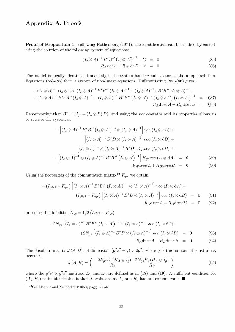
Appendix A: Proofs

Proof of Proposition 1. Following Rothenberg (1971), the identification can be studied by consid-ering the solution of the following system of equations:

(Is ⊗A)−1B∗B∗′(Is ⊗A′

)−1 − Σ = 0 (85)RAvecA+RBvecB − r = 0 (86)

The model is locally identified if and only if the system has the null vector as the unique solution.Equations (85)-(86) form a system of non-linear equations. Differentiating (85)-(86) gives:

− (Is ⊗A)−1 (Is ⊗ dA) (Is ⊗A)−1B∗B∗′ (Is ⊗A)−1 + (Is ⊗A)−1 dB∗B∗′ (Is ⊗A)−1 +

+ (Is ⊗A)−1B∗dB∗′ (Is ⊗A)−1 − (Is ⊗A)−1B∗B∗′(Is ⊗A′

)−1 (Is ⊗ dA′

) (Is ⊗A′

)−1 = 0(87)RAdvecA+RBdvecB = 0(88)

Remembering that B∗ = (Igs + (Is ⊗B)D), and using the vec operator and its properties allows usto rewrite the system as

−[(Is ⊗A)−1B∗B∗′

(Is ⊗A′

)−1 ⊗ (Is ⊗A)−1]vec (Is ⊗ dA) +[

(Is ⊗A)−1B∗D ⊗ (Is ⊗A)−1]vec (Is ⊗ dB) +[

(Is ⊗A)−1 ⊗ (Is ⊗A)−1B∗D]Kgsvec (Is ⊗ dB) +

−[(Is ⊗A)−1 ⊗ (Is ⊗A)−1B∗B∗′

(Is ⊗A′

)−1]Kgsvec (Is ⊗ dA) = 0 (89)

RAdvecA+RBdvecB = 0 (90)

Using the properties of the commutation matrix12 Kgs we obtain

−(Ig2s2 +Kgs

) [(Is ⊗A)−1B∗B∗′

(Is ⊗A′

)−1 ⊗ (Is ⊗A)−1]vec (Is ⊗ dA) +(

Ig2s2 +Kgs

) [(Is ⊗A)−1B∗D ⊗ (Is ⊗A)−1

]vec (Is ⊗ dB) = 0 (91)

RAdvecA+RBdvecB = 0 (92)

or, using the definition Ngs = 1/2(Ig2s2 +Kgs

)−2Ngs

[(Is ⊗A)−1B∗B∗′

(Is ⊗A′

)−1 ⊗ (Is ⊗A)−1]vec (Is ⊗ dA) +

+2Ngs

[(Is ⊗A)−1B∗D ⊗ (Is ⊗A)−1

]vec (Is ⊗ dB) = 0 (93)

RAdvecA+RBdvecB = 0 (94)

The Jacobian matrix J (A,B), of dimension(g2s2 + q

)× 2g2, where q is the number of constraints,

becomes

J (A,B) =(−2NgsE1 (HA ⊗ Ig) 2NgsE2 (HB ⊗ Ig)

RA RB

)(95)

where the g2s2 × g2s2 matrices E1 and E2 are defined as in (18) and (19). A sufficient condition for(A0, B0) to be identifiable is that J evaluated at A0 and B0 has full column rank.

12See Magnus and Neudecker (2007), pagg. 54-56.

28

Proof of Corollary 1. Since the two members of (85) are constituted by block diagonal matrices,the complete system of equations can be re-written in s sub-systems, one for each volatility state, as

A−1B1B′1A−1′ − Σ1 = 0

A−1B2B′2A−1′ − Σ2 = 0

...A−1BsB

′sA−1′ − Σs = 0

where Bi = Ig +BDi and Σi is the matrix of second moments for the error terms in the i-th state ofvolatility. As Corollary 1 is interested on the left block of the Jacobian matrix (17), we only need tocalculate the first differentials with respect to the parameters in A, that become

Ng

[A−1B1B

′1A−1′ ⊗A′

]vecdA = 0

Ng

[A−1B2B

′2A−1′ ⊗A′

]vecdA = 0

...Ng

[A−1BsB

′sA−1′ ⊗A′

]vecdA = 0.

In order to prove the result, it is sufficient to prove that the following system of equations admits thenull vector as the unique possible solution:

Ng

[A−1B1B

′1A−1′ ⊗A′

]x1 = 0

Ng

[A−1B2B

′2A−1′ ⊗A′

]x1 = 0

... (96)Ng

[A−1BsB

′sA−1′ ⊗A′

]x1 = 0.

For simplicity, let define B∗i =[A−1BiB

′iA−1′ ⊗A′

]. If we focus on the first block equation, a possible

solution can be given asx1 = B∗−1

1 Dgq

for any generic g (g − 1) /2× 1 vector q. Substituting this solution into the second block equation, itbecomes

NgB∗2B∗−11 Dgq = 0. (97)

Once proved that the g2 × g (g − 1) /2 matrix NgB∗2B∗−11 Dg has full column rank, the only possible

solution is the vector q = 0. This result, can be easily substituted in all other block equations in (96),proving the result. The aim, thus, is to prove that rank

(NgB

∗2B∗−11 Dg

)= g (g − 1) /2.

Obviously, B∗2 and B∗−11 are non-singular matrices, and the same holds for their product. Moreover,

by definition, rank (Ng) = g (g + 1) /2 while Dg has full column rank g (g − 1) /2. If we define α =D′gB

∗−1′1 B∗′2 and β = Ng, then

rank(NgB

∗2B∗−11 Dg

)= rank

(D′gB

∗−1′1 B∗′2 Ng

)= rank (αβ)

and the proof reduces to demonstrate that, in such particular case, the rank of the product of the twomatrices is equal to the minor of the two ranks. In particular, given that B∗−1′

1 B∗′2 is non singular,rank (α) = rank′g = g (g − 1) /2, and that rank (Ng) = g (g + 1) /2, we need to prove that

rank (αβ) = rank (α) = g2.

The strategy we follow is to consider the linear transformations induced by the two matrices α andβ, and then the composition of the two. In particular, define α : V → W and β : Z → V , then thecomposition of α and β is the function (α β) : Z →W whose outputs are defined by

(α β) (z) = α (β (z)) (98)

29

for z ∈ Z, where Z ⊆ Rg2 , V ⊆ Rg2 , and W ⊆ Rg(g−1)/2. Of course, a sufficient, but not necessary,condition is that β is a surjective linear transformation, or in other words, β (Z) = V . Intuitively, aless stringent sufficient condition, instead, is that α needs to be as much uninjective on the image of βas on V ; more precisely Ker (α) = Ker

(α|Im(β)

), with

(α|Im(β)

)the restriction of α to Im (β), and

where Im (·) and Ker (·) are the image (or range) and kernel (or null space) of a linear transforma-tion, respectively. But being the Im (β) a subspace of V , then Ker

(αΦ|Im(β)

)= Im (β) ∩Ker (α).

Moreover, by definition ker (α) = α′⊥, where α′⊥ is the orthogonal complement13 of α′. Using ourdefinition of α′, its orthogonal complement is defined such that

αα′⊥ = D′gB∗−1′1 B∗′2 B

∗−1′2 B∗′1 Dg (99)

where Dg is the duplication matrix as defined before. The Kernel of α is thus a subspace of Rg2 ofdimension g (g + 1) /2 for which one possible basis can be given by the columns of Dg. Moreover, ifwe remember that β = Ng, and that Ng = DgD

+g , then

Im (β) = span (Ng) = span(DgD

+g

)(100)

where the span of a matrix is the space generated by the columns of that matrix. The image of β isthus a subspace of Rg2 generated by the columns of Dg. The intersection of Im (β) and Ker (α) isthen the space generated by the columns of Dg, which is also equal to the kernel of α.

This result proves that the rank of NgB∗2B∗−11 Dg is effectively full and equal to g (g − 1) /2. The

only possible solution for the system of equations in (97) is thus the vector q = 0, that, once substitutedin all the other equations, proves the final result.

Proof of Proposition 2. Starting from the log-likelihood function in (7), the first differentialbecomes

dl (θ) = tr T ∗ (Is ⊗A)−1 (Is ⊗ dA)− tr T ∗B∗−1 (Is ⊗ dB)D

−12tr[T ∗(Is ⊗ dA′

)B∗−1′B∗−1 (Is ⊗A) Σ

]+

12tr[T ∗(Is ⊗A′

)B∗−1′D

(Is ⊗ dB′

)B∗−1′B∗−1 (Is ⊗A) Σ

]+

12tr[T ∗(Is ⊗A′

)B∗−1′B∗−1 (Is ⊗ dB)DB∗−1 (Is ⊗A) Σ

]−1

2tr[T ∗(Is ⊗A′

)B∗−1′B∗−1 (Is ⊗ dA) Σ

], (101)

using the properties of the vec operator and the Kgs matrix, the first differential becomes

dl (θ) = vec(T ∗(Is ⊗A−1′))′ (HA ⊗ Ig) vecdA− vec

(B∗−1′T ∗D

)′ (HB ⊗ Ig) vecdB

−12vec

(B∗−1′B∗−1 (Is ⊗A) ΣT ∗

)′(HA ⊗ Ig) vecdA

+12vec

(B∗−1′B∗−1 (Is ⊗A) ΣT ∗

(Is ⊗A′

)B∗−1′D

)′(HB ⊗ Ig) vecdB

+12vec

(B∗−1′B∗−1 (Is ⊗A)T ∗Σ

(Is ⊗A′

)B∗−1′D

)′(HB ⊗ Ig) vecdB

−12vec

(B∗−1′B∗−1 (Is ⊗A)T ∗Σ

)′(HA ⊗ Ig) vecdA (102)

but given that T ∗ is diagonal, thus T ∗Σ = ΣT ∗, and the score vector in (66)-(66) immediately follows.13See Luktepohl (2005, pag. 654) for a detailed definition of the orthogonal complement of a matrix.

30

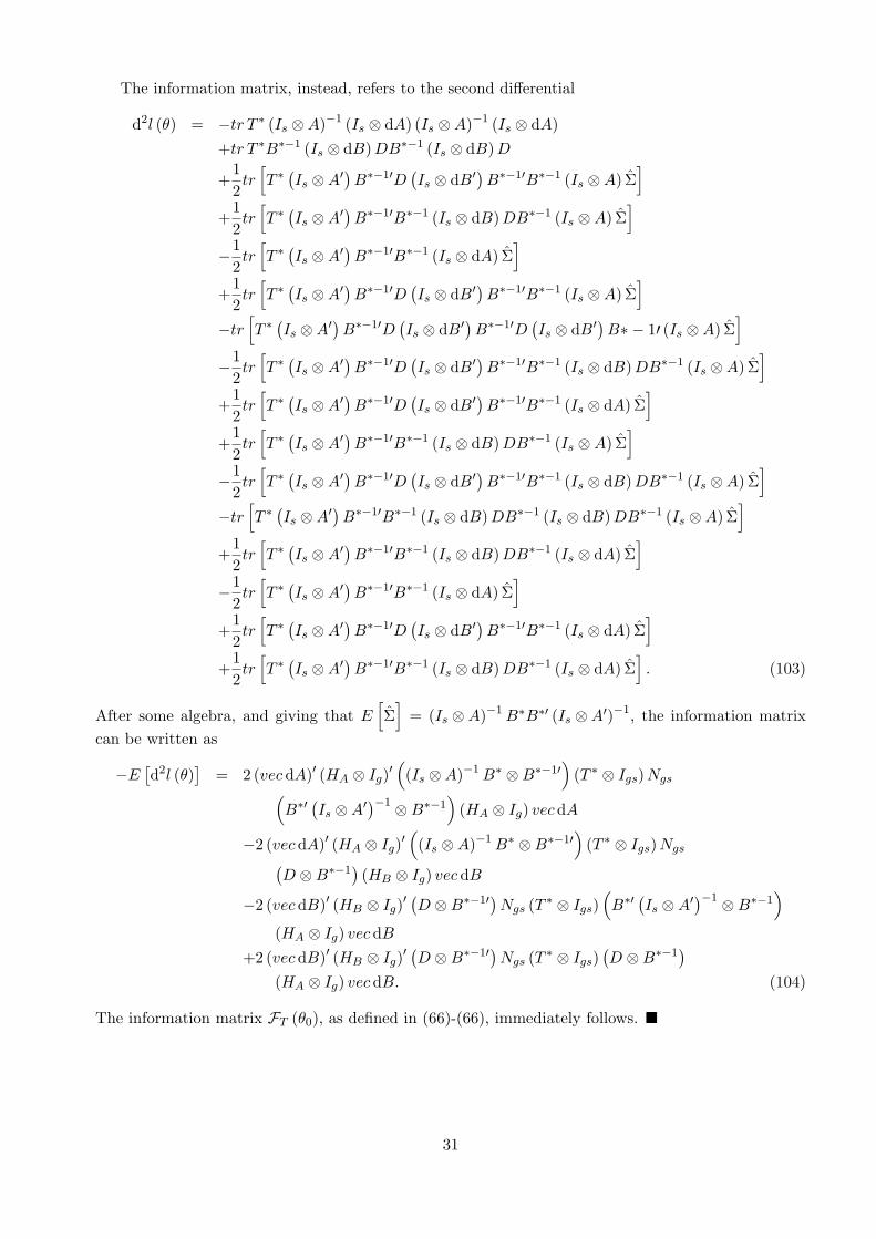
The information matrix, instead, refers to the second differential

d2l (θ) = −tr T ∗ (Is ⊗A)−1 (Is ⊗ dA) (Is ⊗A)−1 (Is ⊗ dA)+tr T ∗B∗−1 (Is ⊗ dB)DB∗−1 (Is ⊗ dB)D

+12tr[T ∗(Is ⊗A′

)B∗−1′D

(Is ⊗ dB′

)B∗−1′B∗−1 (Is ⊗A) Σ

]+

12tr[T ∗(Is ⊗A′

)B∗−1′B∗−1 (Is ⊗ dB)DB∗−1 (Is ⊗A) Σ

]−1

2tr[T ∗(Is ⊗A′

)B∗−1′B∗−1 (Is ⊗ dA) Σ

]+

12tr[T ∗(Is ⊗A′

)B∗−1′D

(Is ⊗ dB′

)B∗−1′B∗−1 (Is ⊗A) Σ

]−tr

[T ∗(Is ⊗A′

)B∗−1′D

(Is ⊗ dB′

)B∗−1′D

(Is ⊗ dB′

)B∗ − 1′ (Is ⊗A) Σ

]−1

2tr[T ∗(Is ⊗A′

)B∗−1′D

(Is ⊗ dB′

)B∗−1′B∗−1 (Is ⊗ dB)DB∗−1 (Is ⊗A) Σ

]+

12tr[T ∗(Is ⊗A′

)B∗−1′D

(Is ⊗ dB′

)B∗−1′B∗−1 (Is ⊗ dA) Σ

]+

12tr[T ∗(Is ⊗A′

)B∗−1′B∗−1 (Is ⊗ dB)DB∗−1 (Is ⊗A) Σ

]−1

2tr[T ∗(Is ⊗A′

)B∗−1′D

(Is ⊗ dB′

)B∗−1′B∗−1 (Is ⊗ dB)DB∗−1 (Is ⊗A) Σ

]−tr

[T ∗(Is ⊗A′

)B∗−1′B∗−1 (Is ⊗ dB)DB∗−1 (Is ⊗ dB)DB∗−1 (Is ⊗A) Σ

]+

12tr[T ∗(Is ⊗A′

)B∗−1′B∗−1 (Is ⊗ dB)DB∗−1 (Is ⊗ dA) Σ

]−1

2tr[T ∗(Is ⊗A′

)B∗−1′B∗−1 (Is ⊗ dA) Σ

]+

12tr[T ∗(Is ⊗A′

)B∗−1′D

(Is ⊗ dB′

)B∗−1′B∗−1 (Is ⊗ dA) Σ

]+

12tr[T ∗(Is ⊗A′

)B∗−1′B∗−1 (Is ⊗ dB)DB∗−1 (Is ⊗ dA) Σ

]. (103)

After some algebra, and giving that E[Σ]

= (Is ⊗A)−1B∗B∗′ (Is ⊗A′)−1, the information matrixcan be written as

−E[d2l (θ)

]= 2 (vecdA)′ (HA ⊗ Ig)′

((Is ⊗A)−1B∗ ⊗B∗−1′

)(T ∗ ⊗ Igs)Ngs(

B∗′(Is ⊗A′

)−1 ⊗B∗−1)

(HA ⊗ Ig) vecdA

−2 (vecdA)′ (HA ⊗ Ig)′(

(Is ⊗A)−1B∗ ⊗B∗−1′)

(T ∗ ⊗ Igs)Ngs(D ⊗B∗−1

)(HB ⊗ Ig) vecdB

−2 (vecdB)′ (HB ⊗ Ig)′(D ⊗B∗−1′)Ngs (T ∗ ⊗ Igs)

(B∗′

(Is ⊗A′

)−1 ⊗B∗−1)

(HA ⊗ Ig) vecdB+2 (vecdB)′ (HB ⊗ Ig)′

(D ⊗B∗−1′)Ngs (T ∗ ⊗ Igs)

(D ⊗B∗−1

)(HA ⊗ Ig) vecdB. (104)

The information matrix FT (θ0), as defined in (66)-(66), immediately follows.

31