Hysteresis-based analysis of overland metal transport

HYDROLOGICAL PROCESSESHydrol. Process. 17, 1579–1606 (2003)Published online 24 March 2003 in Wiley InterScience (www.interscience.wiley.com). DOI: 10.1002/hyp.1200

Hysteresis-based analysis of overland metal transport

Surendra Kumar Mishra,1* J. J. Sansalone2 and Vijay P. Singh2

1 National Institute of Hydrology, Jalviggan Bhawan, Roorkee 247 667, UP, India2 Department of Civil and Environmental Engineering, Louisiana State University, Baton Rouge, LA 70803-6405, USA

Abstract:

Introducing a concept of equivalent mass depth of flow, this study describes the phenomenon of non-point sourcepollutant (metal) transport for pavement (or overland) flow in analogy with wave propagation in wide open channels.Hysteretic and normal mass rating curves are developed for runoff rate and mass of 12 dissolved and particulate-boundmetal elements (pollutants) using the rainfall-runoff and water quality data of the 15 ð 20 m2 instrumented pavementin Cincinnati, USA. Normal mass rating curves developed for easy computation of pollutant load are found to be ofa form similar to Manning’s, which is valid for open channel flows. Based on the hysteresis analysis, wave typesfor dissolution and mixing of particulate-bound metals are identified. The analysis finds that the second-order partial-differential equation normally used for metal transport does not have the efficacy to describe fully the strong non-linearphenomena such as is described for various metal elements by dynamic waves. In addition, the proportionality conceptof the popular SCS-CN concept is extended for determining the potential maximum metal mass Mp of all the 12elements transported by a rain storm and related to the antecedent dry period (ADP). For the primary metal zincelement, Mp is found to increase with the ADP and vice versa. Copyright 2003 John Wiley & Sons, Ltd.

KEY WORDS mass transport; heavy metals; overland flow; hysteretic transport; normal mass rating curves

INTRODUCTION

Urban highway storm water often contains elevated levels of heavy metals and particles (Sansalone andBuchberger, 1997; Sansalone et al., 1998; Li et al., 1999). Heavy metals, like Pb, Cd, Cu, Ni, Zn, and Cr, canpose acute and chronic threats to receiving water bodies and soils. In receiving water, the dissolved fraction ofthese heavy metals has the potential for acute and long-term chronic toxicity for aquatic life. Unlike organiccompounds, heavy metals are not degraded in the environment. With the recent signature of the Final Rulefor Phase II Storm Water US National Pollutant Discharge Elimination System (NPDES) regulations on 29October 1999, issues related to heavy metals in roadway storm water have now come into direct focus atthe national regulatory level. In the urban highway environment, heavy metals are generated primarily fromthe abrasion of metal-containing vehicular parts, including the abrasive interaction of tyres against pavement,leaching of heavy metals from infrastructure, oil and grease leakage and industrial discharges Lygren et al.,1984; Muschack, 1990; (Ball et al., 1991; Armstrong, 1994). Pavement and vehicle part abrasion are sourcesof solids that can range from colloidal- to gravel-size particles abraded from pavement. These solids washoff in lateral pavement sheet flow during rainfall-runoff events as part of a heterogeneous mixture of heavymetals, organic compounds, oil and grease, and partition into particulate-bound metals and dissolved metals(Sansalone and Buchberger, 1997).

Traffic and roadway maintenance activities are major sources of particulates and solids that are eitherinitially abraded heavy metals that dissolve in the rainfall of low pH and low alkalinity or solids that act asa substrate to which dissolved heavy metals can partition (Sansalone and Buchberger, 1997). The sources of

* Correspondence to: Dr Surendra Kumar Mishra, National Institute of Hydrology, Jalviggan Bhawan, Roorkee 247 667, UP, India.E-mail: [email protected]

Received 4 September 2000Copyright 2003 John Wiley & Sons, Ltd. Accepted 9 July 2002

1580 S. K. MISHRA, J. J. SANSALONE AND V. P. SINGH

these solids and abraded heavy metals include construction/re-construction activities, maintenance operationsthat include application of grit and salt (coated with anti-caking materials containing heavy metals) in northernclimates, pavement degradation, littering, spillage, and vehicular-infrastructure abrasion. Within the categoryof vehicular-infrastructure abrasion, tyre–pavement interaction generates a significant amount of particulatematter. Abraded pavement accounts for 40–50% and abraded tyres account for 20–30% of the total particulatematter generated (Kobriger and Geinopolos, 1984). Most of these abraded solids and particulates contain heavymetals. Abraded tyre particles have a mean diameter of 20 µm, a density of 1Ð5–1Ð7 g cm3, and are the majorsources of Zn and Cd (Sansalone and Tribouillard, 1999).

Heavy metal concentrations in urban runoff can range from essentially background levels to milligram/litrelevels during a single rainfall-runoff event. Since the concentration of hydrologically transported constituentscan vary by orders of magnitude during a single runoff event, a single index designated as event meanconcentration (EMC) is often used to characterize concentrations. EMC represents a flow average concentrationfor the event and, at a particular site, it can vary depending on average daily traffic, vehicles during storm,rain intensity, previous dry days, and climate conditions (Sansalone and Buchberger, 1997; Sansalone et al.,1998; Li et al., 1999). Although the benefits of EMC data include simplicity and economics, drawbacksof EMC data include the inability of such data to quantify the temporal and hysteretic variation of waterquality parameters.

The hysteretic nature of dissolution of heavy metals and mixing of particulate-bound metals with the rainwater has not yet been studied and reported in the literature. There is also a need to develop normal ratingcurves for computing the mass concentration from the available information on rainfall, similar to the normalrating curves used for converting stages to discharges in open channels. Thus, the objective of this paper isto study the hysteretic nature of mass transport employing the concept of hysteresis used in the description oflooped rating curves in open channel hydraulics, develop normal mass rating curves, analogous to the normalflow rating curves, and suggest a procedure for computing the potential maximum mass transported by a rainstorm utilizing the rainfall-runoff-water quality data derived from an instrumented paved stretch of Mill CreekExpressway of I-75 (area: 300 m2) in Cincinnati, USA.

FLOW RATING CURVES

The rating curves in open channel hydraulics provide vital hydrological information, namely the discharge,from measured stage for use in planning, design, operation, and management of water resource projects. Therating curves can be either single- or double-valued, depending on the flow behaviour. The single-valued ratingcurves are much more popular in hydrological practice and research than the double-valued rating curves,also known as looped or hysteretic rating curves. The hysteresis-based hydraulic literature reveals (Henderson,1966; Cunge et al., 1980; Ponce, 1989; Mishra and Seth, 1996; Jain et al., 1996; Mishra et al. 1997; Mishraand Singh, 1999a) that hysteresis is a manifestation of channel storage and/or channel roughness and directlyrelates to the flood wave attenuation. After Henderson (1966), the hysteretic flow behaviour has continuouslybeen a matter of research (Cunge et al., 1980; French, 1985; Ponce, 1989; Perumal, 1994; Mishra and Seth,1994, 1996; Jain et al., 1996; Mishra et al. 1997; Mishra and Singh, 1999a). Using non-dimensional hysteresisas an index, Mishra and Singh (1999a) described flood waves (Table I) in artificial and in natural channels.In Table I, Fo is the Froude number and O� is the dimensionless wave number (Ponce and Simons, 1977).Hysteresis � is computed as (Mishra and Seth, 1994, 1996; Jain et al., 1996; Mishra et al., 1996, 1997; Mishraand Singh, 1999a)

� D 1

2

∫ T

0

(q

dh

dt� h

dq

dt

)dt �1�

Copyright 2003 John Wiley & Sons, Ltd. Hydrol. Process. 17, 1579–1606 (2003)

HYSTERESIS-BASED ANALYSIS OF OVERLAND METAL TRANSPORT 1581

Table I. Criteria for wave types (source: Mishra and Seth (1994,1996))

Wave type Hysteresis �(dimensionless)

Wave number O� and O�Fo

(dimensionless)Phase difference

� (radians)

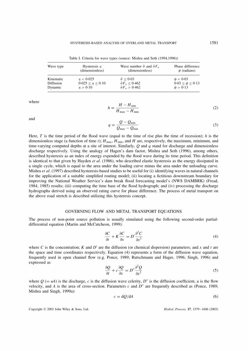
Kinematic � < 0Ð025 O� � 0Ð03 � < 0Ð03Diffusion 0Ð025 � � � 0Ð10 O�Fo � 0Ð462 0Ð03 � � � 0Ð13Dynamic � > 0Ð10 O�Fo > 0Ð462 � > 0Ð13

where

h D H � Hmin

Hmax � Hmin�2�

and

q D Q � Qmin

Qmax � Qmin�3�

Here, T is the time period of the flood wave (equal to the time of rise plus the time of recession); h is thedimensionless stage (a function of time t); Hmax, Hmin, and H are, respectively, the maximum, minimum, andtime-varying computed depths at a site of interest. Similarly, Q and q stand for discharge and dimensionlessdischarge respectively. Using the analogy of Hagen’s dam factor, Mishra and Seth (1996), among others,described hysteresis as an index of energy expended by the flood wave during its time period. This definitionis identical to that given by Hayden et al. (1986), who described elastic hysteresis as the energy dissipated ina single cycle, which is equal to the area under the loading curve minus the area under the unloading curve.Mishra et al. (1997) described hysteresis-based studies to be useful for (i) identifying waves in natural channelsfor the application of a suitable simplified routing model; (ii) locating a fictitious downstream boundary forimproving the National Weather Service’s dam break flood forecasting model’s (NWS DAMBRK) (Fread,1984, 1985) results; (iii) computing the time base of the flood hydrograph; and (iv) processing the dischargehydrographs derived using an observed rating curve for phase difference. The process of metal transport onthe above road stretch is described utilizing this hysteresis concept.

GOVERNING FLOW AND METAL TRANSPORT EQUATIONS

The process of non-point source pollution is usually simulated using the following second-order partial-differential equation (Martin and McCutcheon, 1999):

∂C

∂tC K

∂C

∂xD D0 ∂

2C

∂x2 �4�

where C is the concentration; K and D0 are the diffusion (or chemical dispersion) parameters; and x and t arethe space and time coordinates respectively. Equation (4) represents a form of the diffusion wave equation,frequently used in open channel flow (e.g. Ponce, 1989; Rutschmann and Hager, 1996; Singh, 1996) andexpressed as

∂Q

∂tC c

∂Q

∂xD D00 ∂

2Q

∂x2 �5�

where Q (D uA) is the discharge, c is the diffusion wave celerity, D00 is the diffusion coefficient, u is the flowvelocity, and A is the area of cross-section. Parameters c and D00 are frequently described as (Ponce, 1989;Mishra and Singh, 1999a):

c D dQ/dA �6�



andD00 D Qo/�2SoW� �7�

where Qo is the reference flow, So is the bed slope, and W is the channel width, which is equal to unity fora unit width rectangular channel. Equation (6) is the popular Seddon speed formula. Since Equations (4) and(5) parallel each other, it is possible to describe the non-point source pollutant transport in overland flow (orimpervious urban sheet flow), analogous to the flow in wide rectangular open channels, if C in Equation (4)is replaced by a term equivalent to the product of flow depth and velocity. In a similar vein, the dynamicprocess of metal transport can be described using the equations analogous to the one-dimensional dynamicwave equations, described by the continuity and momentum equations, which, respectively, are

∂h

∂tC u

∂h

∂xC h

∂u

∂xD 0 �8�

and∂h

∂tC u

∂u

∂xC g

∂h

∂xC g�Sf � So� D 0 �9�

valid for a unit-width wide rectangular channel. Here, h is the depth of flow, g is the gravitational acceleration,and Sf is the friction slope, which is described by Manning’s equation:

u D 1

nR2/3S1/2

f �10�

where R is the hydraulic radius (equal to h for a wide rectangular channel) and n is Manning’s roughnesscoefficient.

Owing to their highly non-linear nature, Equations (8)–(10) do not yield an exact analytical solution,and approximate methods (e.g. linear and numerical methods) are, therefore, often resorted to. Ponce andSimons (1977) and Menendez and Norscini (1982) solved these equations for wide rectangular channelsusing a linear perturbation theory. Ponce and Simons (1977) derived propagation characteristics of kinematic,diffusion, steady-dynamic, gravity, and dynamic waves in open channel flow. These characteristics includedwave celerity and attenuation defined by logarithmic decrement. Menendez and Norscini (1982) characterizedthese waves by wave celerity and phase difference and showed a link between logarithmic decrement andphase difference. A more general relationship between logarithmic decrement and phase speed was derivedby Kundzewicz and Dooge (1989). Singh (1996) provided an overview of these studies. The work of Price(1973, 1985) is also notable, in that he provided a more generalized solution of the St Venant equationsproviding a relationship between attenuation and wave speed. Mishra and Singh (2001) described the wavecharacteristics using the hysteresis concept as follows:

Ocr D š 1p2

(

1

F2o

� �2

)2

C �2

1/2

C 1

F2o

� �2

1/2

�11�

υ D �2

� Ý 1p2

(1

F2o

� �2

)2

C �2

1/2

� 1

F2o

C �2

1/2

1 š 1p2

(

1

F2o

� �2

)2

C �2

1/2

C 1

F2o

� �2

1/2 �12�



� D tan�1

� Ý 1p2

(1

F2o

� �2

)2

C �2

1/2

� 1

F2o

C �2

1/2

š 1p2

(1

F2o

� �2

)2

C �2

1/2

C 1

F2o

� �2

1/2 �13�

where Oc D c/uo and Ocr represents the dimensionless relative celerity, ��D 1/ O�F2o� is the kinematic wave

number, υ is the logarithmic decrement, uo is the normal flow velocity, and the dimensionless wave numberis described as

O� D �2/L��ho/So� �14�

where ho is the normal flow depth. These derivations conformed to those given by Ponce and Simons (1977)and Menendez and Norscini (1982), who have described in detail the wave characteristics employing theabove derivations.

CONCEPT OF EQUIVALENT MASS DEPTH OF FLOW

The above dynamic wave equations (Equations (8) and (9)) are the result of mass and momentum conservation.To describe the mechanism of metal transport analogous to open channel wave propagation, it is necessarythat the flow depth h be replaced by a term describing mass of the transported metal in such a way that themass and momentum of flow in a channel remain conserved. To this end, a hypothetical flow in a real channelof equivalent mass depth of flow he is considered and described as

he�t� D m�t�

Aw�15�

where he(t) is the equivalent mass depth of flow at time t, m(t) is the mass of the metal transported at time t, is the metal density, and Aw is the area of the overland. In the present hypothetical flow, the flow velocityu is taken as equal to the velocity of the real flow (direct surface runoff) [L3T�1] divided by the area [L2] ofthe watershed, for the flow velocity directly impacts the mass transport. Thus, u and he act exactly analogousto the two orthogonal components, u and h respectively, of the full dynamic wave equations (Equations (8)and (9)), leading to the description of characteristics of metal transport phenomenon by Equations (11)–(13),including the establishment of mass rating curves for m (or he) (Equation (15)) and u. Here, it is to be notedthat, in open channel hydraulics, rating curves are used to convert stage h to flow velocity u (or discharge),whereas in non-point source metal transport (e.g. on an overland where the flow is described primarily bysheet flow), these can be of use in determination of the amount of mass transported by the known velocityof flow that is taken to be equivalent to the rate of rainfall excess or direct runoff.

RELATION BETWEEN EQUIVALENT DEPTH OF MASS AND CONCENTRATION

The relation, described by Equation (15), can be shown equivalent to the concentration of flow that is moreconvincingly used in environmental engineering literature as below:

Concentration is defined as

C D Mass of the transported metal

Volume of the solution�16�



or alternatively


Metal density ð Volume of the solution�17�

C in Equation (16) has the dimension of [ML�3], whereas in Equation (17) it is non-dimensional. The non-dimensional C is generally expressed in parts per million. Equation (17) can also be written in terms of therates of mass and flow as


Metal density ð Rate of direct surface runoff ð t�18�

where t is the time interval, the direct surface runoff is the solution, and the ratio of transported mass tot represents the rate of mass transported. Division of the numerator and denominator of the right-hand sideof Equation (18) by the area of the watershed yields

C D [m/�Aw�]/�ut� �19�

orC D he/�ut� �20�

which describes C as the ratio of the equivalent depth of mass [L] to the flow displacement [L], which,however, assumes the rate of rainfall excess equivalent to the overland flow velocity.

APPLICATION

Study area

An experimental urban watershed in Cincinnati (USA) of 15 ð 20 m2 asphalt pavement of I-75 (at milestone2Ð6), which is a major north–south interstate, was selected for collecting rainfall-runoff data during 1995–97(Sansalone and Buchberger, 1997). The runoff on the highway site located at the upstream end of an urbanwatershed finally drains into Mill Creek. The runoff from the selected stretch of 300 m2 is contributed bythe four southbound lanes, an exit lane, and a paved shoulder, all draining to a grassy V-section medianat a transverse pavement cross-slope of 0Ð020 m m�1 as shown in the plan view of Figure 1a and b. Theflow on the longitudinal pavement slope of 0Ð004 is primarily characterized by sheet flow, and the land useis characterized as urban (industrial, commercial, residential). The storm water runoff diverted through theepoxy-coated converging slab, a 2Ð54 cm diameter Parshall flume, and a 2 m long 25Ð4 cm diameter PVC pipeto a 2000 l storage tank was measured at regular 1 min intervals using an automated 24 bottle sampler withpolypropylene bottles. The rainfall was recorded using a tipping bucket gauge in increments of 0Ð254 mm.Cincinnati receives an annual average 1020 mm of rainfall and 420 mm of snow. High rainfall occurs in March(average of 106 mm) and July (average of 104 mm), and the highest snowfall occurs in January (average of150 mm) (Anon, 1982). The average winter and summer temperatures are 0 °C and 23Ð4 °C respectively. Thewater quality data at every 2 min interval were collected during rainfall-runoff events at the experimentalsite and samples were analysed for dissolved and particulate-bound metals for the rainfall-runoff events of 17June, 7 July, and 8 August 1996 (Sansalone and Buchberger, 1997; Sansalone et al., 1998; Li et al., 1999).An example set of hydrologic and water quality data for the event of 8 August 1996 is shown in Table IIwith the linearly interpolated values of water quality data.



Figure 1. Plan view of (a) I-75 highway site at Cincinnati, and (b) experimental setup at I-75 site



Table II. Example data for the dissolved solids of Zn of 8 August 1996 event

Time(min)

Rainfallintensity

(mm h�1)

Runoff rate(mm h�1)

Dissolvedmass(µg)

Equivalent massdepth he

(10�9 mm)

Time(min)

Rainfallintensity

(mm h�1)

Runoff rate(mm h�1)

Dissolvedmass(µg)

Equivalent massdepth he

(10�9 mm)

0 2Ð04 0Ð00 0Ð00 0Ð00 24 18Ð36 21Ð81 18 261 8Ð531 2Ð04 0Ð00 0Ð00 0Ð00 25 18Ð36 21Ð09 18 094 8Ð452 2Ð04 0Ð00 0Ð00 0Ð00 26 18Ð36 19Ð09 17 927 8Ð373 2Ð04 0Ð00 0Ð00 0Ð00 27 18Ð36 18Ð43 23 084 10Ð784 2Ð04 0Ð00 0Ð00 0Ð00 28 9Ð18 20Ð97 28 241 13Ð185 2Ð04 0Ð00 0Ð00 0Ð00 29 9Ð18 18Ð05 30 945 14Ð456 2Ð04 0Ð00 0Ð00 0Ð00 30 9Ð18 15Ð25 33 650 15Ð717 2Ð04 0Ð01 0Ð00 0Ð00 31 9Ð18 12Ð72 31 879 14Ð888 2Ð04 0Ð08 0Ð00 0Ð00 32 9Ð18 13Ð04 30 108 14Ð069 18Ð36 0Ð18 0Ð00 0Ð00 33 9Ð18 11Ð29 30 347 14Ð17

10 18Ð36 0Ð59 15 824 7Ð39 34 6Ð12 10Ð92 30 587 14Ð2811 18Ð36 5Ð80 92 783 43Ð32 35 6Ð12 7Ð97 29 863 13Ð9412 18Ð36 12Ð26 169 743 79Ð25 36 6Ð12 7Ð76 29 138 13Ð6013 18Ð36 13Ð32 125 357 58Ð52 37 0Ð00 5Ð74 24 149 11Ð2714 73Ð45 19Ð79 80 971 37Ð80 38 0Ð00 5Ð49 19 159 8Ð9415 73Ð45 36Ð47 179 588 83Ð84 39 0Ð00 3Ð42 15 695 7Ð3316 55Ð08 56Ð26 278 204 129Ð88 40 0Ð00 2Ð07 12 230 5Ð7117 91Ð81 56Ð06 212 691 99Ð30 41 0Ð00 2Ð27 13 764 6Ð4318 110Ð17 68Ð56 147 179 68Ð71 42 0Ð00 1Ð93 15 297 7Ð1419 91Ð81 78Ð29 93 083 43Ð46 43 0Ð00 1Ð79 16 830 7Ð8620 18Ð36 75Ð49 38 987 18Ð20 44 0Ð00 1Ð93 14 575 6Ð8021 36Ð72 56Ð08 31 658 14Ð78 45 0Ð00 1Ð25 12 320 5Ð7522 18Ð36 39Ð74 24 329 11Ð36 46 0Ð00 1Ð36 10 384 4Ð8523 18Ð36 28Ð86 21 295 9Ð94 47 0Ð00 0Ð62 8448 3Ð94

Development of looped mass rating curves

The water quality analysis for dissolved and particulate-bound metals was performed for 12 metal elements,viz. Zn, Cd, Pb, Ni, Mn, Fe, Cr, Mg, Al, Ca, Cu, and Na. Table II summarizes the dissolved mass of Zn inmicrograms. The values of the mass of the dissolved solids were converted to equivalent depth of mass he,using Equation (15). The runoff rate in Table II represents the direct surface runoff observed at the outlet ofthe 15 m ð 20 m micro urban watershed. It can be computed using a suitable rainfall-runoff model (Singh,1988). Thus, the advantage of developing rating curves for pollutants lies in the fact that, for a given amountof rainfall intensity, the mass of either dissolved or particulate-bound metals can be easily determined.

With the above assumption of the direct surface runoff observed at the outlet to be equivalent to the velocityof overland flow, rating curves analogous to those in open channels were developed for the dissolved and theparticulate-bound metal elements described above, and these are shown in Figures 2 and 3 respectively forthe event of 8 August 1996. It is noted that the y-axes of the rating curves for various elements shown inFigures 2 and 3 represent the mass of the flow (Table II), rather than he. It is apparent from these figures thatseveral metals (e.g. Pb, Mn, Mg, Cu, and Na in Figure 2) exhibit a relation that is tantamount to steady-stateflow rating curves observed in open channels. All other dissolved and particulate-bound elements show mildto strong loops in the rating curves. Data points that deviate from the looped shape in a few plots in Figure 2(e.g. the plots for Zn, Cd, and Mn, among others) are attributed to the multiplicity of peaks of the runoffhydrograph. This is exemplified in Figures 4 and 5 using the data of Table II and the event of 7 July 1996 forthe dissolved Zn. Figure 5 exhibits the formation of three loops in the rating curves in accordance with thethree discernible runoff hydrograph peaks. Such a phenomenon of mixed waves is typical in open channelflows, and the hysteretic behaviour (or loop formation) depends greatly on the initial (input) flow and channelstorage conditions (Mishra and Singh, 1999a). The underlying difference, however, is that the natural flow



20 40 60 800

Runoff rate (mm/hr)

3.E+05

2.E+05

1.E+05

0.E+00

Zn

(µg

)

20 40 60 800

Runoff rate (mm/hr)

6.E+02

4.E+02

2.E+02

0.E+00

Cd

(µg

)

20 40 60 800

Runoff rate (mm/hr)

3.E+04

2.E+04

1.E+04

0.E+00

20 40 60 800

Runoff rate (mm/hr)

4.E+03

2.E+03

3.E+03

1.E+03

0.E+00

Pb

(µg

)N

i (µg

)

20 40 60 800

Runoff rate (mm/hr)

3.E+04

2.E+042.E+04

1.E+045.E+030.E+00

Mn

(µg

)

20 40 60 800

Runoff rate (mm/hr)

6.E+04

4.E+04

2.E+04

0.E+00

Fe

(µg

)

20 40 60 800

Runoff rate (mm/hr)

2.E+04

1.E+04

5.E+03

0.E+00

Cr

(µg

)

20 40 60 800

Runoff rate (mm/hr)

5.E+054.E+053.E+052.E+051.E+050.E+00

Mg

(µg

)

20 40 60 800

Runoff rate (mm/hr)

3.E+05

2.E+052.E+05

1.E+05

0.E+005.E+04

20 40 60 800

Runoff rate (mm/hr)

8.E+06

4.E+06

6.E+06

2.E+06

0.E+00

Al (

µg)

Ca

(µg

)

20 40 60 800

Runoff rate (mm/hr)

2.E+04

5.E+03

1.E+04

0.E+00

Cu

(µg

)

20 40 60 800

Runoff rate (mm/hr)

3.E+062.E+06

1.E+062.E+06

0.E+005.E+05N

a (µ

g)

Figure 2. Relation between runoff rate and the mass of dissolved metals for 8 August 1996 event



20 40 60 800

Runoff rate (mm/hr)

3.E+05

2.E+05

1.E+05

0.E+00

Zn

(µg

)

20 40 60 800

Runoff rate (mm/hr)

6.E+02

4.E+02

2.E+02

0.E+00

Cd

(µg

)

20 40 60 800

Runoff rate (mm/hr)

3.E+04

2.E+04

1.E+04

0.E+00

20 40 60 800

Runoff rate (mm/hr)

4.E+03

2.E+03

3.E+03

1.E+03

0.E+00

Pb

(µg

)N

i (µg

)

20 40 60 800

Runoff rate (mm/hr)

3.E+04

2.E+042.E+04

1.E+045.E+030.E+00

Mn

(µg

)

20 40 60 800

Runoff rate (mm/hr)

6.E+04

4.E+04

2.E+04

0.E+00

Fe

(µg

)

20 40 60 800

Runoff rate (mm/hr)

20 40 60 800

Runoff rate (mm/hr)

20 40 60 800

Runoff rate (mm/hr)

20 40 60 800

Runoff rate (mm/hr)

20 40 60 800

Runoff rate (mm/hr)

20 40 60 800

Runoff rate (mm/hr)

2.E+04

1.E+04

5.E+03

0.E+00

Cr

(µg

)

5.E+054.E+053.E+052.E+051.E+050.E+00

Mg

(µg

)3.E+05

2.E+052.E+05

1.E+05

0.E+005.E+04

8.E+06

4.E+06

6.E+06

2.E+06

0.E+00

Al (

µg)

Ca

(µg

)

2.E+04

5.E+03

1.E+04

0.E+00

Cu

(µg

)

1.E+058.E+04

4.E+046.E+04

0.E+002.E+04N

a (µ

g)

Figure 3. Relation between runoff rate and the mass of particulate-bound metals for 8 August 1996 event



0

20

40

60

80

100

120

140

0 10 20 30 40 50 60 70 80

Runoff rate (mm/hr)

Aug. 8, 1996

h (

10-9

mm

)

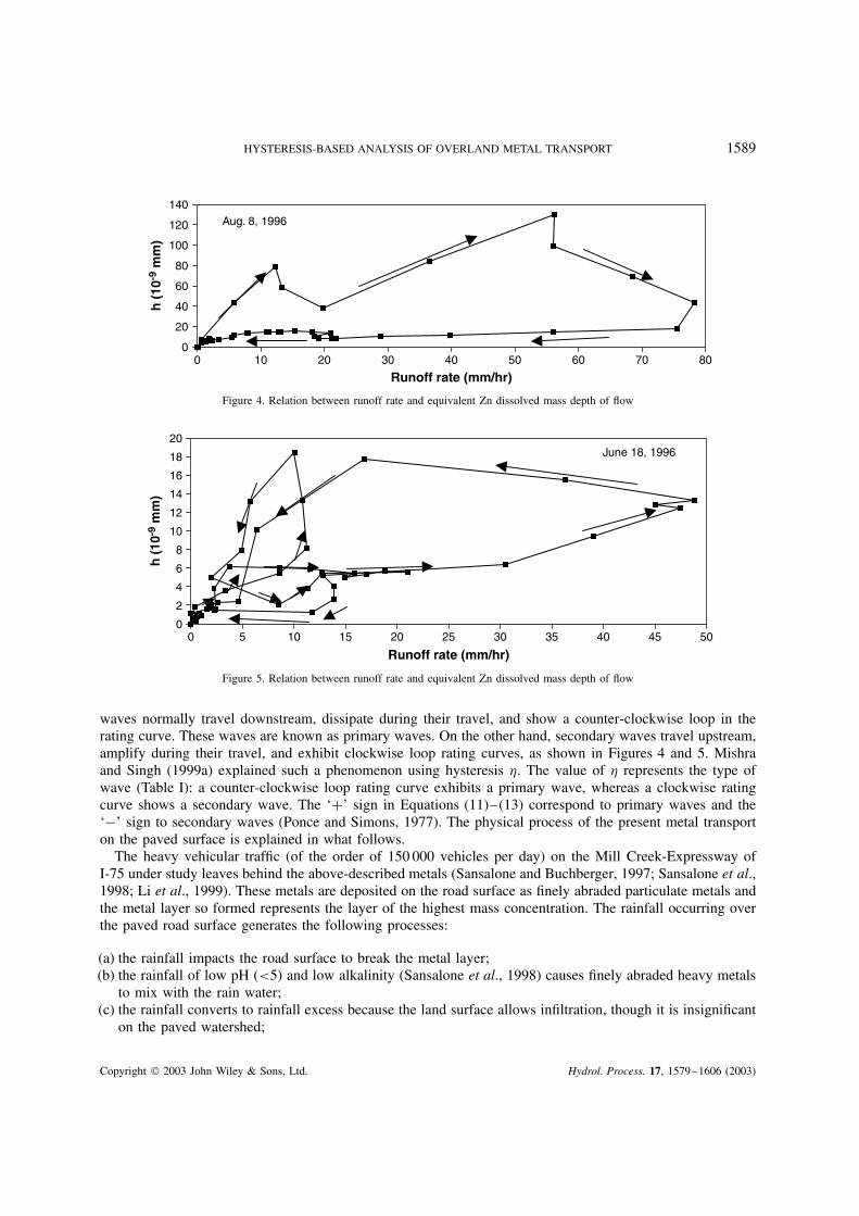
Figure 4. Relation between runoff rate and equivalent Zn dissolved mass depth of flow

0

2

4

6

8

10

12

14

16

18

20

0 5 10 15 20 25 30 35 40 45 50

June 18, 1996

h (

10-9

mm

)

Runoff rate (mm/hr)

Figure 5. Relation between runoff rate and equivalent Zn dissolved mass depth of flow

waves normally travel downstream, dissipate during their travel, and show a counter-clockwise loop in therating curve. These waves are known as primary waves. On the other hand, secondary waves travel upstream,amplify during their travel, and exhibit clockwise loop rating curves, as shown in Figures 4 and 5. Mishraand Singh (1999a) explained such a phenomenon using hysteresis �. The value of � represents the type ofwave (Table I): a counter-clockwise loop rating curve exhibits a primary wave, whereas a clockwise ratingcurve shows a secondary wave. The ‘C’ sign in Equations (11)–(13) correspond to primary waves and the‘�’ sign to secondary waves (Ponce and Simons, 1977). The physical process of the present metal transporton the paved surface is explained in what follows.

The heavy vehicular traffic (of the order of 150 000 vehicles per day) on the Mill Creek-Expressway ofI-75 under study leaves behind the above-described metals (Sansalone and Buchberger, 1997; Sansalone et al.,1998; Li et al., 1999). These metals are deposited on the road surface as finely abraded particulate metals andthe metal layer so formed represents the layer of the highest mass concentration. The rainfall occurring overthe paved road surface generates the following processes:

(a) the rainfall impacts the road surface to break the metal layer;(b) the rainfall of low pH (<5) and low alkalinity (Sansalone et al., 1998) causes finely abraded heavy metals

to mix with the rain water;(c) the rainfall converts to rainfall excess because the land surface allows infiltration, though it is insignificant

on the paved watershed;



(d) the rainfall excess builds up storage on the road surface before the start of the direct surface runoff; thehigher the storage, the greater will be the rate of direct surface runoff, and vice versa;

(e) the low pH and poorly buffered water storage or pondage on the road surface allows dissolution (ordiffusion) of metals;

(f) the breaking up of the metal layer leads to the mixing of particulate-bound and dissolved metals with therainfall excess.

Both dissolved and particulate-bound metals are carried by the direct surface runoff to the outlet. Theprocess of dissolution (or molecular diffusion or dispersion) is usually described by a linear Fick’s first law,which describes the phenomenon of molecular diffusion as to be directly proportional to the concentrationgradient; the higher the gradient, the higher will be the rate of dissolution, and vice versa. It is expressedmathematically as (Martin and McCutcheon, 1999):

ϑ D �D0 ∂C

∂x�21�

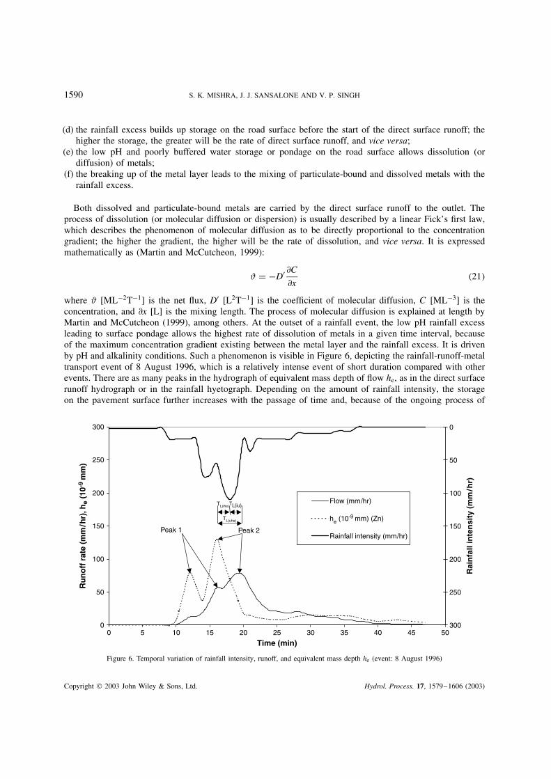
where ϑ [ML�2T�1] is the net flux, D0 [L2T�1] is the coefficient of molecular diffusion, C [ML�3] is theconcentration, and ∂x [L] is the mixing length. The process of molecular diffusion is explained at length byMartin and McCutcheon (1999), among others. At the outset of a rainfall event, the low pH rainfall excessleading to surface pondage allows the highest rate of dissolution of metals in a given time interval, becauseof the maximum concentration gradient existing between the metal layer and the rainfall excess. It is drivenby pH and alkalinity conditions. Such a phenomenon is visible in Figure 6, depicting the rainfall-runoff-metaltransport event of 8 August 1996, which is a relatively intense event of short duration compared with otherevents. There are as many peaks in the hydrograph of equivalent mass depth of flow he, as in the direct surfacerunoff hydrograph or in the rainfall hyetograph. Depending on the amount of rainfall intensity, the storageon the pavement surface further increases with the passage of time and, because of the ongoing process of

0

50

100

150

200

250

300

0 5 10 15 20 25 30 35 40 45 50

0

50

100

150

200

250

300

Rai

nfa

ll in

ten

sity

(m

m/h

r)

Flow (mm/hr)

he (10-9 mm) (Zn)

Rainfall intensity (mm/hr)Peak 1 Peak 2

TL(ihe)TL(iu)

TL(uhe)

Ru

no

ff r

ate

(mm

/hr)

, he

(10-

9 m

m)

Time (min)

Figure 6. Temporal variation of rainfall intensity, runoff, and equivalent mass depth he (event: 8 August 1996)



0

20

40

60

80

100

120 0

20

40

60

80

100

120

Rai

nfa

ll in

ten

sity

(m

m/h

r)

Flow (mm/hr)

he (10-9 mm) (Zn)

Rainfall intensity (mm/hr)Peak 4

0 10 20 30 40 50 60

Ru

no

ff r

ate

(mm

/hr)

, he

(10-

9 m

m)

Time (min)

Peak 3

Figure 7. Temporal variation of rainfall intensity, runoff, and equivalent mass depth he (event: 18 June 1996)

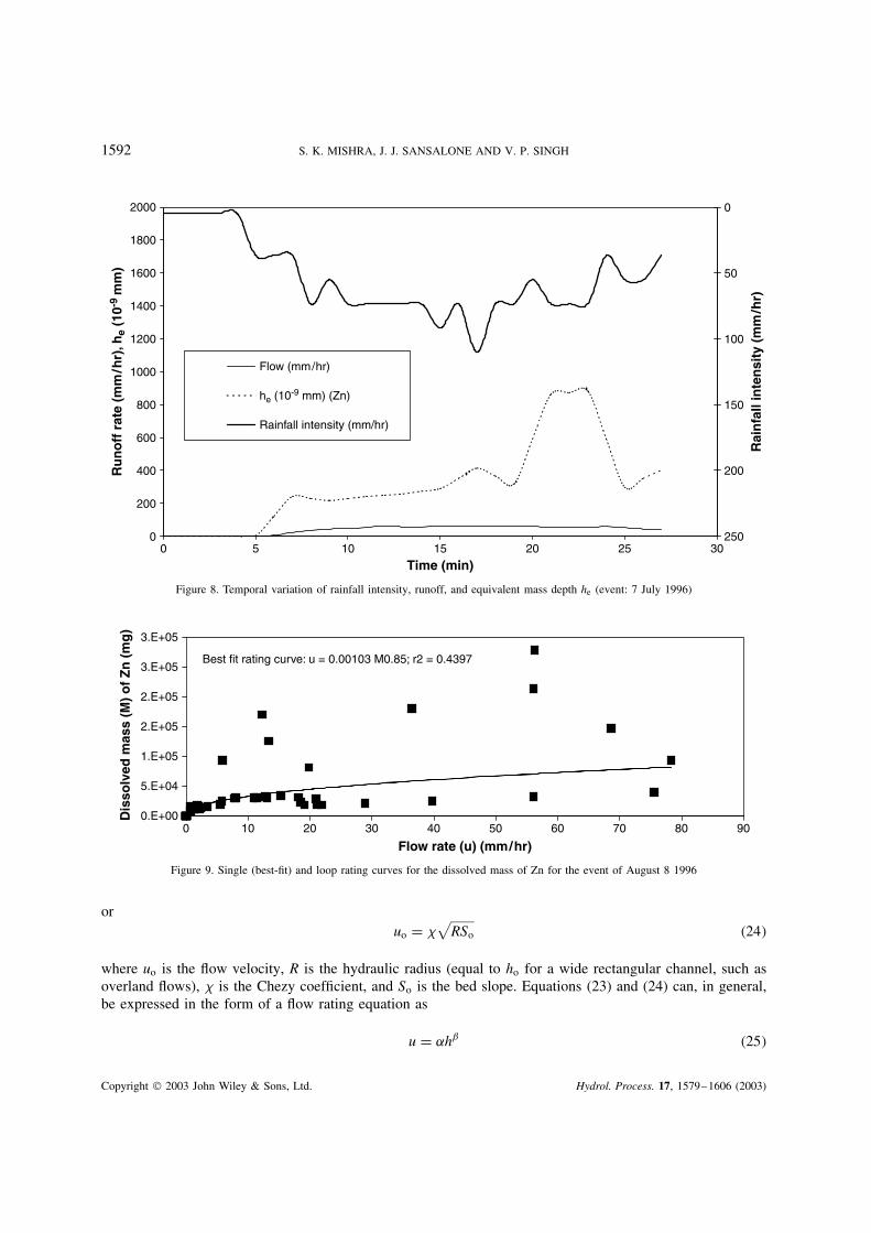
dissolution, the concentration gradient decreases with time, which, in turn, decreases the rate of dissolutionof metal mass or the mass of the metal during the given time interval (D m(t)). The difference between therate of runoff and the rate of dissolution produces a time lag (or phase lag) between them. A phenomenon ofpositive time lag is apparent in Figure 7, which depicts the event of 18 June 1996. The slow rising trend ofthe rainfall hyetograph results in the slow piling up of water on the paved surface, allowing more time forwater to stay on the surface, leading to slow rate of dissolution with the passage of time and, consequently,a positive phase lag between the rate of runoff and he, as seen in Figures 7 and 8, in which the peaks ofhe occur later than the peaks of the direct surface runoff. Here, it is noted that the event of 8 August 1996exhibits the case of a negative time lag.

Development of normal mass rating curves

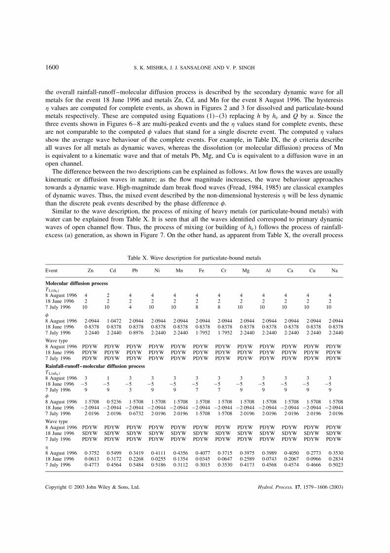
The use of normal flow rating curves is more common in practice than the looped rating curves. On similargrounds, it is useful to develop normal mass rating curves for water quality analyses. To that end, best-fitcurves for all the above-described three events and for all the dissolved and particulate-bound metal elementswere derived from the data, as shown in Figures 2 and 4 and exemplified in Figure 9 for the event of 8August 1996. These rating curves are described using the following power relation:

u D amb �22�

where u is the rate of direct surface runoff, m is the mass of the dissolved or particulate-bound metals, anda and b are the mass rating coefficient and exponent respectively. Such a relationship (Equation (22)) wasadopted for the reason of its resemblance with Manning’s or Chezy’s friction laws, which are widely used inopen channel hydraulics and expressed mathematically as

uo D 1

nR2/3S1/2

o �23�



0

200

400

600

800

1000

1200

1400

1600

1800

2000

0 5 10 15 20 25 30

0

50

100

150

200

250

Rai

nfa

ll in

ten

sity

(m

m/h

r)

Flow (mm/hr)

he (10-9 mm) (Zn)

Rainfall intensity (mm/hr)

Time (min)

Ru

no

ff r

ate

(mm

/hr)

, he

(10-

9 m

m)

Figure 8. Temporal variation of rainfall intensity, runoff, and equivalent mass depth he (event: 7 July 1996)

0.E+00

5.E+04

1.E+05

2.E+05

2.E+05

3.E+05

3.E+05

0 10 20 30 40 50 60 70 80 90

Dis

solv

ed m

ass

(M)

of

Zn

(m

g)

Best fit rating curve: u = 0.00103 M0.85; r2 = 0.4397

Flow rate (u) (mm/hr)

Figure 9. Single (best-fit) and loop rating curves for the dissolved mass of Zn for the event of August 8 1996

oruo D

√RSo �24�

where uo is the flow velocity, R is the hydraulic radius (equal to ho for a wide rectangular channel, such asoverland flows), is the Chezy coefficient, and So is the bed slope. Equations (23) and (24) can, in general,be expressed in the form of a flow rating equation as

u D ˛hˇ �25�



where u and h represent the channel flow velocity and depth respectively, and parameters ˛ and ˇ representthe flow rating coefficient and exponent respectively, depending on the channel and flow characteristicsas follows:

˛ D 1

nS1/2

o �26�

and ˇ D 2/3 (Manning’s friction) or 0Ð5 (Chezy’s friction) depending on the type of flow (laminar, turbulent,or transition). Here, it is noted that the dimensionless relative celerity Ocr (Equations (11)– (14)) of the openchannel flow is equal to ˇ. In a similar vein, the exponent b of Equation (22) describes the kinematicwave celerity of mass transport of both dissolved and particulate-bound metals. Furthermore, the term D0 inEquation (21) describing the process of dissolution (or molecular diffusion) inheres resistance to moleculardiffusion (Martin and McCutcheon, 1999), and is, thus, analogous to friction in open channel flows. Therefore,a concept of equivalent mass roughness, analogous to Manning’s roughness, representing the dissolution ofmetals (dissolved) or mixing (particulate-bound) metals is considered. It is expressed mathematically as

ne D S1/2o /ab �27�

derivable from Equations (15), (22), and (23). From Equation (27), the product of ne and b should form aconstant for a given watershed. The computed parameters a and b, the equivalent mass roughness ne, and theproduct of ne and b for all events and all dissolved and particulate-bound metals are given in Tables III andIV. The average values of these parameters are shown in Table V. In these computations, the bed slope istaken as 0Ð02, the area of the watershed is 300 m2, and the equivalent depth of mass he is taken in 10�9 mm. Itis apparent from Table III that parameter b varies from 0Ð52 to 1Ð91. As shown in the histogram of parameterb (Figure 10) developed using the data of Table III, most values fall in the range (1Ð02, 1Ð24), a close rangeof variation. It is noted that b D 1Ð0 represents a straight-line relationship between the rate of surface runoff uand the equivalent mass depth of flow he. In surface water flows, or overland flow in particular, the range ofvariation of parameter b is equivalent to 50–75% of turbulent flows, described by Manning’s friction (Ponce,1989). Parameter a (Table III), however, shows a wider range of variation than does parameter b and exhibitsa link with parameter b, as shown in Figure 11. Apparently, parameter a varies inversely with parameter b.Thus, parameter a is also sensitive to the variation in types of flow, as described above, and, therefore, theproduct of ne and b (Equation (27)) will also vary (as seen in Table IV), with the change in parameter b.

The actual amount of the metal transported in a given time interval also depends on other factors, suchas the actual number of vehicles passing through the stretch before the occurrence of the rain storm. Duringheavy rainy days, it is more likely that the number of vehicles will be less than that during dry days, and viceversa. Thus can be realized from Figure 8, which depicts the event of 7 July 1996. Apparently, for the sameorder of peak rainfall intensity, the peak of the he-hydrograph (Figure 8) is several times larger than that of8 August 1996 (Figure 6). Thus, the number of antecedent dry days influences significantly the number ofvehicles that have passed through the road stretch before the start of the rain and, in turn, the potential depthof the metal layer, which is analysed later.

Wave analysis

Similar to the waves in open channels, the wave characteristics of the events shown in Figures 6–8 aredetermined using the phase difference and non-dimensional hysteresis �. Following the work of Mishra andSeth (1996), the phase difference � is computed as

� D 2

T[tp�he� � tp�u�] �28�

where � is in radians; T is in hours; tp�he� (min), is the time of rise of the he-wave and tp�u� (min) is the time ofrise of the u-wave. Menendez and Norscini (1983) described � as a kinematic parameter that drives attenuation.



Tabl

eII

I.C

ompu

tatio

nof

mas

sra

ting

para

met

ersa

�uD

aMb�

Eve

ntZ

nC

dPb

Ni

Mn

Fe

ba

ba

ba

ba

ba

ba

Dis

solv

edso

lids

8A

ugus

t19

960Ð8

51Ð0

3E�

031Ð2

03Ð1

4E�

021Ð1

66Ð8

3E�

041Ð7

85Ð0

4E�

051Ð9

15Ð7

4E�

071Ð3

63Ð4

8E�

0518

June

1996

1Ð29

4Ð83E

�05

1Ð01

1Ð52E

�01

0Ð98

8Ð12E

�03

1Ð01

1Ð29E

�02

1Ð06

1Ð04E

�03

0Ð61

3Ð19E

�02

7Ju

ly19

961Ð1

21Ð1

2E�

050Ð9

23Ð4

9E�

020Ð6

64Ð6

5E�

020Ð7

81Ð4

9E�

021Ð1

61Ð9

0E�

040Ð9

78Ð5

4E�

04

Par

ticu

late

-bou

ndso

lids

8A

ugus

t19

961Ð1

67Ð8

0E�

040Ð9

67Ð1

9E�

011Ð2

73Ð0

6E�

031Ð1

25Ð8

6E�

021Ð1

74Ð0

4E�

031Ð1

84Ð6

8E�

0518

June

1996

1Ð11

2Ð69E

�03

1Ð14

6Ð12E

�01

1Ð05

2Ð21E

�02

1Ð01

1Ð26E

�01

0Ð85

6Ð90E

�02

0Ð96

9Ð04E

�04

7Ju

ly19

960Ð6

43Ð9

3E�

020Ð6

41Ð0

7EC

000Ð7

07Ð3

0E�

020Ð5

25Ð3

1E�

011Ð0

01Ð9

0E�

020Ð9

94Ð2

5E�

04

Cr

Mg

Al

Ca

Cu

Na

ba

ba

ba

ba

ba

ba

Dis

solv

edso

lids

8A

ugus

t19

961Ð1

52Ð1

5E�

031Ð8

08Ð1

5E�

091Ð2

72Ð0

6E�

051Ð6

21Ð1

4E�

091Ð8

63Ð2

4E�

061Ð8

15Ð2

5E�

1018

June

1996

1Ð22

2Ð78E

�03

1Ð07

6Ð57E

�05

0Ð93

1Ð03E

�03

1Ð11

3Ð70E

�06

1Ð10

3Ð49E

�03

1Ð09

8Ð55E

�06

7Ju

ly19

960Ð5

84Ð3

3E�

010Ð9

01Ð4

8E�

040Ð7

14Ð1

4E�

031Ð0

23Ð7

5E�

061Ð0

19Ð2

7E�

040Ð8

96Ð7

6E�

05

Par

ticu

late

-bou

ndso

lids

8A

ugus

t19

961Ð0

21Ð1

3E�

011Ð1

41Ð3

2E�

041Ð0

94Ð1

7E�

041Ð0

58Ð5

0E�

051Ð3

71Ð7

9E�

031Ð0

74Ð1

9E�

0418

June

1996

0Ð98

2Ð40E

�01

0Ð77

7Ð08E

�03

1Ð01

1Ð97E

�03

0Ð85

9Ð06E

�04

1Ð00

4Ð51E

�02

1Ð02

1Ð19E

�03

7Ju

ly19

960Ð8

24Ð4

0E�

010Ð8

31Ð8

3E�

030Ð7

96Ð1

1E�

030Ð7

41Ð3

3E�

030Ð7

76Ð1

6E�

020Ð5

92Ð3

7E�

02

aa

and

bar

eth

era

ting

curv

eco

effic

ient

and

expo

nent

resp

ectiv

ely.



Tabl

eIV

.C

ompu

tati

onof

rati

ngpa

ram

eter

sa

Eve

ntZ

nC

dPb

Ni

Mn

FeC

rM

gA

lC

aC

uN

a

Dis

solv

edso

lids

ne

8A

ugus

t19

963Ð2

2EC

033Ð9

4EC

021Ð5

8EC

042Ð1

8EC

063Ð0

4EC

086Ð6

2EC

054Ð8

5EC

031Ð4

6EC

107Ð9

6EC

055Ð2

1EC

104Ð6

3EC

072Ð3

3EC

1118

June

1996

3Ð60E

C05

4Ð00E

C01

6Ð80E

C02

4Ð74E

C02

7Ð29E

C03

4Ð36E

C01

4Ð90E

C03

1Ð19E

C05

4Ð38E

C03

2Ð39E

C06

2Ð48E

C03

9Ð55E

C05

7Ju

ly19

968Ð5

0EC

051Ð2

5EC

023Ð5

6EC

011Ð7

8EC

025Ð7

5EC

046Ð1

3EC

032Ð8

8EC

002Ð7

5EC

044Ð9

4EC

021Ð7

1EC

066Ð6

0EC

035Ð8

1EC

04

ne

b

8A

ugus

t19

961Ð7

0EC

044Ð1

4EC

031Ð5

4EC

057Ð2

2EC

071Ð2

9EC

109Ð6

4EC

064Ð6

7EC

045Ð0

8EC

119Ð6

8EC

061Ð2

5EC

121Ð8

0EC

098Ð0

9EC

1218

June

1996

4Ð52E

C06

2Ð91E

C02

4Ð67E

C03

3Ð44E

C03

5Ð90E

C04

1Ð45E

C02

5Ð41E

C04

9Ð77E

C05

2Ð71E

C04

2Ð09E

C07

2Ð15E

C04

8Ð05E

C06

7Ju

ly19

967Ð7

8EC

067Ð5

4EC

021Ð2

9EC

028Ð3

2EC

025Ð6

6EC

054Ð0

9EC

049Ð0

3EC

001Ð6

1EC

052Ð0

1EC

031Ð2

7EC

074Ð7

9EC

043Ð3

3EC

05

Par

ticu

late

-bou

ndm

etal

sn

e8

Aug

ust

1996

1Ð40E

C04

7Ð02E

C00

5Ð32E

C03

1Ð62E

C02

2Ð75E

C03

2Ð46E

C05

5Ð59E

C01

7Ð67E

C04

1Ð99E

C04

8Ð43E

C04

1Ð31E

C04

1Ð84E

C04

18Ju

ne19

963Ð3

3EC

031Ð6

3EC

013Ð2

2EC

024Ð9

2EC

014Ð9

4EC

015Ð6

6EC

032Ð2

8EC

013Ð6

4EC

023Ð1

1EC

033Ð7

6EC

031Ð3

1EC

025Ð4

6EC

037

July

1996

3Ð98E

C01

1Ð45E

C00

2Ð62E

C01

1Ð86E

C00

3Ð11E

C02

1Ð32E

C04

6Ð95E

C00

1Ð74E

C03

4Ð47E

C02

1Ð71E

C03

4Ð00E

C01

5Ð41E

C01

ne

b

8A

ugus

t19

961Ð3

7EC

054Ð6

1EC

016Ð4

4EC

041Ð4

8EC

032Ð7

3EC

042Ð5

0EC

064Ð1

4EC

027Ð2

4EC

051Ð6

9EC

056Ð6

4EC

051Ð9

3EC

051Ð5

1EC

0518

June

1996

2Ð95E

C04

1Ð52E

C02

2Ð55E

C03

3Ð60E

C02

2Ð64E

C02

3Ð73E

C04

1Ð56E

C02

1Ð67E

C03

2Ð26E

C04

2Ð01E

C04

9Ð30E

C02

4Ð07E

C04

7Ju

ly19

961Ð4

1EC

025Ð1

4EC

001Ð0

3EC

025Ð1

7EC

002Ð2

0EC

039Ð1

5EC

043Ð4

9EC

018Ð9

2EC

032Ð1

2EC

037Ð3

3EC

031Ð7

9EC

021Ð7

2EC

02

a

isth

em

ass

dens

ity;

h eis

the

equi

vale

ntm

ass

dept

h(1

0�9m

m);

ne

isth

eeq

uiva

lent

roug

hnes

s;a

and

bar

era

ting

curv

eco

effic

ient

and

expo

nent

resp

ectiv

ely.



Tabl

eV

.C

ompu

tatio

nof

aver

age

valu

esof

ratin

gpa

ram

eter

sfo

rdi

ssol

ved

and

part

icul

ate-

boun

dso

lidsa

Para

met

erZ

nC

dPb

Ni

Mn

FeC

rM

gA

lC

aC

uN

a

Dis

solv

edso

lids

b1Ð0

91Ð0

40Ð9

31Ð1

91Ð3

80Ð9

80Ð9

81Ð2

60Ð9

71Ð2

51Ð3

21Ð2

6a

3Ð63E

�04

7Ð28E

�02

1Ð84E

�02

9Ð28E

�03

4Ð10E

�04

1Ð09E

�02

1Ð46E

�01

7Ð12E

�05

1Ð73E

�03

2Ð48E

�06

1Ð47E

�03

2Ð54E

�05

ne

4Ð05E

C05

1Ð86E

C02

5Ð50E

C03

7Ð27E

C05

1Ð01E

C08

2Ð23E

C05

3Ð24E

C03

4Ð87E

C09

2Ð66E

C05

1Ð74E

C10

1Ð54E

C07

7Ð76E

C10

ne

b4Ð1

1EC

061Ð7

3EC

035Ð2

8EC

042Ð4

1EC

074Ð2

9EC

093Ð2

2EC

063Ð3

5EC

041Ð6

9EC

113Ð2

4EC

064Ð1

6EC

116Ð0

2EC

082Ð7

1EC

12

Par

ticu

late

-bou

ndso

lids

b0Ð9

70Ð9

11Ð0

10Ð8

81Ð0

11Ð0

40Ð9

40Ð9

10Ð9

60Ð8

81Ð0

50Ð8

9a

1Ð43E

�02

8Ð00E

�01

3Ð27E

�02

2Ð39E

�01

3Ð07E

�02

4Ð59E

�04

2Ð64E

�01

3Ð01E

�03

2Ð83E

�03

7Ð74E

�04

3Ð62E

�02

8Ð44E

�03

ne

5Ð79E

C03

8Ð25E

C00

1Ð89E

C03

7Ð09E

C01

1Ð04E

C03

8Ð83E

C04

2Ð86E

C01

2Ð62E

C04

7Ð83E

C03

3Ð00E

C04

4Ð45E

C03

7Ð98E

C03

ne

b5Ð5

7EC

046Ð8

0EC

012Ð2

4EC

046Ð1

5EC

029Ð9

1EC

038Ð7

9EC

052Ð0

1EC

022Ð4

6EC

056Ð4

6EC

042Ð3

0EC

056Ð4

8EC

046Ð4

0EC

04

a

isth

em

ass

dens

ity;

ne

isth

eeq

uiva

lent

roug

hnes

s;a

and

bar

era

ting

curv

eco

effic

ient

and

expo

nent

resp

ectiv

ely.



0

2

4

6

8

10

12

0.58 0.80 1.02 1.24 1.46 1.68 More

Parameter 'b'

Fre

qu

ency

Figure 10. Histogram showing the variation of parameter b

1.0E−10

1.0E−08

1.0E−06

1.0E−04

1.0E−02

1.0E+00

0.00 0.50 1.00 1.50 2.00 2.50

b

a

Best-fit line:y = 794.13e − 13.873 x; r2 = 0.6527

Figure 11. Variation of the rating coefficient a with the rating exponent b

Mishra and Singh (1999a) derived a mathematical expression linking the phase difference � with the non-dimensional hysteresis �. The computation of � is exemplified for the selected four discrete peaks shown inFigures 6 and 7 for the dissolved metal Zn. The wave phenomenon of molecular diffusion pertinent to thepresent case study can be described in three components: (1) rainfall-runoff process; (2) molecular diffusionprocess; (3) rainfall-runoff–molecular diffusion process. To that end, three time lags for easily discerniblepeaks are considered, as shown in Figure 6 for peak no. 2: (a) time lag between the peaks of rainfall andrunoff, designated as TL�iu�; (b) time lag between rainfall and equivalent mass depth of flow he; designated asTL�ihe�; and (c) time lag between the runoff and equivalent mass depth of flow, designated as TL�uhe�. TL�iu�

describes the lag between peak rainfall intensity and the peak runoff rate; it represents the storage effect andhelps describe the average wave celerity of the dynamic rainfall-runoff process. If the direct surface runoffobserved at the outlet of the watershed is accounted for the time lag TL�iu�, it will represent the rainfall excessover the watershed, where the dissolution or mixing of metals with water takes place. Thus, the time lagbetween the peak rainfall intensity and he (D TL�ihe�� indirectly represents the lag between the rates of rainfallexcess and molecular diffusion; the greater the lag, the more dynamic will be the process, and vice versa. Thetime lag between runoff and he�D TL�uhe�� considers both the rainfall-runoff and molecular diffusion processesand is the end result observed at the outlet of the watershed. For convenience of description, the time to peak



rainfall intensity is designated as tp�i�, time to peak runoff as tp�u�, and time to peak he as tp�he�. Thus:

TL�iu� D tp�u� � tp�i� �29�

TL�ihe� D tp�he� � tp�i� �30�

TL�uhe� D tp�he� � tp�u� �31�

For the discrete peaks example of Figures 6 and 7, the computed time lags are given in Table VI. In thistable, the time period corresponds to the time of rise plus the time of recession of the he-wave. Using thesetime lags, the above processes are described below.

Using TL�iu�, the average wave celerity is computed as (Mishra and Seth, 1996):

Average wave celerity D x/Tt �32�

where x is the reach length and Tt is the time of travel [D TL�iu�], which is equivalent to the storagerouting coefficient of reservoir routing used in catchment routing. For the selected events the average wavecelerity varies from 0Ð79 to 1Ð80 m s�1. In Table VI, the negative time lags indicate that the he-wave precedesthe rainfall intensity i-, or runoff u-wave, leading to a negative phase difference describing the analogousprocess of secondary waves in open channels. Based on the phase difference criteria (Table I), the waves ofmolecular diffusion and the rainfall-runoff–molecular diffusion are described to be either a primary dynamicwave (PDYW) or a secondary dynamic wave (SDYW).

Similar to the above, computations for all 12 dissolved and particulate-bound metals were made for all theabove three rainfall-runoff events (Table VII), and the corresponding time to peaks of rainfall, runoff, and he

Table VI. Characteristics of the selected wave events for metal transporta

Waveno.

Time topeak rainfall

intensitytp�i� (min)

Time topeak

runofftp�u� (min)

Time topeak

he, tp�he�

(min)

Timeperiod

T (min)

Rainfall-runoff process Molecular diffusion Rainfall-runoff–molecular diffusion

TL�iu�

(min)Average wave

celerity (m s�1)TL�ihe�

(min)�

(radian)Wavetype

TL�uhe�

(min)�

(radian)Wavetype

1 15 17 12 7 2 1Ð7952 �3 �2Ð6928 SDYW �5 �4Ð4880 SDYW2 18 19 16 8 1 0Ð7854 �2 �1Ð5708 SDYW �3 �2Ð3562 SDYW3 14 15 17 7 1 0Ð8976 3 2Ð6928 PDYW 2 1Ð7952 PDYW4 44 45 47 5 1 1Ð2566 3 3Ð7699 PDYW 2 2Ð5133 PDYW

a TL�iu� is the time difference between rainfall-peak and direct surface runoff peak; TL�ihe� is the time difference between peak rainfall andpeak equivalent mass depth of flow; TL�uhe� is the time difference between direct surface runoff and equivalent mass depth of flow he; Tis the time period; � is the phase difference; PDYW stands for primary dynamic wave for metal transport; SDYW stands for secondarydynamic wave for metal transport.

Table VII. Description of rainfall-runoff events

Event Ta (min) TL�iu� (min) Average wave celerity(x/TL�iu�� (m s�1)

Wavelength D Av.wave celerity ð T (m)

8 August 1996 12 1 0Ð333 239Ð7618 June 1996 15 7 0Ð048 43Ð207 July 1996 28 1 0Ð333 559Ð44

a Time period is based on the direct surface runoff hydrograph.



Table VIII. Times to peak rainfall intensity, runoff, and equivalent mass depth he

Event tpi (min) tp�u� (min) tp�he� (min)

Zn Cd Pb Ni Mn Fe Cr Mg Al Ca Cu Na

Dissolved solids8 August 1996 18 19 16 16 20 20 16 20 20 20 20 20 20 2018 June 1996 23 30 25 25 26 25 25 31 27 25 25 25 25 257 July 1996 17 18 23 25 25 27 27 25 23 27 27 27 23 23

Particulate-bound metals8 August 1996 18 19 22 20 22 22 22 22 22 22 22 22 22 2218 June 1996 23 30 25 25 25 25 25 25 25 25 25 25 25 257 July 1996 17 18 27 27 21 27 27 25 25 27 27 27 27 27

Table IX. Wave description for dissolved solids

Event Zn Cd Pb Ni Mn Fe Cr Mg Al Ca Cu Na

Molecular diffusion processTL�ihe�8 August 1996 �2 �2 2 2 �2 2 2 2 2 2 2 218 June 1996 2 2 3 2 2 8 4 2 2 2 2 27 July 1996 6 8 8 10 10 8 6 10 10 10 6 6

�8 August 1996 �1Ð0472 �1Ð0472 1Ð0472 1Ð0472 �1Ð0472 1Ð0472 1Ð0472 1Ð0472 1Ð0472 1Ð0472 1Ð0472 1Ð047218 June 1996 0Ð8378 0Ð8378 1Ð2566 0Ð8378 0Ð8378 3Ð3510 1Ð6755 0Ð8378 0Ð8378 0Ð8378 0Ð8378 0Ð83787 July 1996 1Ð3464 1Ð7952 1Ð7952 2Ð2440 2Ð2440 1Ð7952 1Ð3464 2Ð2440 2Ð2440 2Ð2440 1Ð3464 1Ð3464

Wave type8 August 1996 SDYW SDYW PDYW PDYW SDYW PDYW PDYW PDYW PDYW PDYW PDYW PDYW18 June 1996 PDYW PDYW PDYW PDYW PDYW PDYW PDYW PDYW PDYW PDYW PDYW PDYW7 July 1996 PDYW PDYW PDYW PDYW PDYW PDYW PDYW PDYW PDYW PDYW PDYW PDYW

Rainfall-runoff–molecular diffusion processTL�uhe�8 August 1996 �3 �3 1 1 �3 1 1 1 1 1 1 118 June 1996 �5 �5 �4 �5 �5 1 �3 �5 �5 �5 �5 �57 July 1996 5 7 7 9 9 7 5 9 9 9 5 5

�8 August 1996 �1Ð5708 �1Ð5708 0Ð5236 0Ð5236 �1Ð5708 0Ð5236 0Ð5236 0Ð5236 0Ð5236 0Ð5236 0Ð5236 0Ð523618 June 1996 �2Ð0944 �2Ð0944 �1Ð6755 �2Ð0944 �2Ð0944 0Ð4189 �1Ð2566 �2Ð0944 �2Ð0944 �2Ð0944 �2Ð0944 �2Ð09447 July 1996 1Ð1220 1Ð5708 1Ð5708 2Ð0196 2Ð0196 1Ð5708 1Ð1220 2Ð0196 2Ð0196 2Ð0196 1Ð1220 1Ð1220

Wave type8 August 1996 SDYW SDYW PDYW PDYW SDYW PDYW PDYW PDYW PDYW PDYW PDYW PDYW18 June 1996 SDYW SDYW SDYW SDYW SDYW PDYW SDYW SDYW SDYW SDYW SDYW SDYW7 July 1996 PDYW PDYW PDYW PDYW PDYW PDYW PDYW PDYW PDYW PDYW PDYW PDYW

�8 August 1996 0Ð4488 0Ð1907 0Ð0518 0Ð1345 0Ð1905 0Ð3224 0Ð3553 0Ð0609 0Ð2265 0Ð1922 0Ð0401 0Ð119818 June 1996 0Ð5065 0Ð4618 0Ð4153 0Ð3132 0Ð2309 0Ð1391 0Ð6301 0Ð2861 0Ð3705 0Ð3218 0Ð3605 0Ð27307 July 1996 0Ð1505 0Ð3972 0Ð4007 0Ð4541 0Ð0225 0Ð2325 0Ð2725 0Ð4055 0Ð5000 0Ð2920 0Ð2377 0Ð4003

are given in Table VIII. It is noted that, in Table VII, the time period T is computed from the direct surfacerunoff hydrograph corresponding to the discrete highest rainfall intensity of the event. The computed time topeaks (Table VIII) correspond to this discrete event. The wave description for these events is given in Table IX.It is seen that the processes of molecular diffusion of Zn, Cd, and Mn elements are analogous to secondarydynamic waves in open channels and the other elements exhibit primary dynamic wave phenomena. However,



the overall rainfall-runoff–molecular diffusion process is described by the secondary dynamic wave for allmetals for the event 18 June 1996 and metals Zn, Cd, and Mn for the event 8 August 1996. The hysteresis� values are computed for complete events, as shown in Figures 2 and 3 for dissolved and particulate-boundmetals respectively. These are computed using Equations (1)–(3) replacing h by he and Q by u. Since thethree events shown in Figures 6–8 are multi-peaked events and the � values stand for complete events, theseare not comparable to the computed � values that stand for a single discrete event. The computed � valuesshow the average wave behaviour of the complete events. For example, in Table IX, the � criteria describeall waves for all metals as dynamic waves, whereas the dissolution (or molecular diffusion) process of Mnis equivalent to a kinematic wave and that of metals Pb, Mg, and Cu is equivalent to a diffusion wave in anopen channel.

The difference between the two descriptions can be explained as follows. At low flows the waves are usuallykinematic or diffusion waves in nature; as the flow magnitude increases, the wave behaviour approachestowards a dynamic wave. High-magnitude dam break flood waves (Fread, 1984, 1985) are classical examplesof dynamic waves. Thus, the mixed event described by the non-dimensional hysteresis � will be less dynamicthan the discrete peak events described by the phase difference �.

Similar to the wave description, the process of mixing of heavy metals (or particulate-bound metals) withwater can be explained from Table X. It is seen that all the waves identified correspond to primary dynamicwaves of open channel flow. Thus, the process of mixing (or building of he� follows the process of rainfall-excess (u) generation, as shown in Figure 7. On the other hand, as apparent from Table X, the overall process

Table X. Wave description for particulate-bound metals

Event Zn Cd Pb Ni Mn Fe Cr Mg Al Ca Cu Na

Molecular diffusion processTL�ihe�8 August 1996 4 2 4 4 4 4 4 4 4 4 4 418 June 1996 2 2 2 2 2 2 2 2 2 2 2 27 July 1996 10 10 4 10 10 8 8 10 10 10 10 10


Wave type8 August 1996 PDYW PDYW PDYW PDYW PDYW PDYW PDYW PDYW PDYW PDYW PDYW PDYW18 June 1996 PDYW PDYW PDYW PDYW PDYW PDYW PDYW PDYW PDYW PDYW PDYW PDYW7 July 1996 PDYW PDYW PDYW PDYW PDYW PDYW PDYW PDYW PDYW PDYW PDYW PDYW

Rainfall-runoff–molecular diffusion processTL�uhe�8 August 1996 3 1 3 3 3 3 3 3 3 3 3 318 June 1996 �5 �5 �5 �5 �5 �5 �5 �5 �5 �5 �5 �57 July 1996 9 9 3 9 9 7 7 9 9 9 9 9�8 August 1996 1Ð5708 0Ð5236 1Ð5708 1Ð5708 1Ð5708 1Ð5708 1Ð5708 1Ð5708 1Ð5708 1Ð5708 1Ð5708 1Ð570818 June 1996 �2Ð0944 �2Ð0944 �2Ð0944 �2Ð0944 �2Ð0944 �2Ð0944 �2Ð0944 �2Ð0944 �2Ð0944 �2Ð0944 �2Ð0944 �2Ð09447 July 1996 2Ð0196 2Ð0196 0Ð6732 2Ð0196 2Ð0196 1Ð5708 1Ð5708 2Ð0196 2Ð0196 2Ð0196 2Ð0196 2Ð0196

Wave type8 August 1996 PDYW PDYW PDYW PDYW PDYW PDYW PDYW PDYW PDYW PDYW PDYW PDYW18 June 1996 SDYW SDYW SDYW SDYW SDYW SDYW SDYW SDYW SDYW SDYW SDYW SDYW7 July 1996 PDYW PDYW PDYW PDYW PDYW PDYW PDYW PDYW PDYW PDYW PDYW PDYW




of the rainfall-runoff–molecular process is described by both primary and secondary dynamic waves. Themixing of all the metals during the 18 June 1996 event is described by secondary dynamic waves. This impliesthat the he-wave precedes the u-wave and the former follows the rainfall intensity i-wave. This is becausethe mixing primarily occurs over the paved surface and the direct surface runoff is further lagged because ofstorage effects in routing, leading to the precedence of the he-wave.

Parallel to the work of Ponce et al. (1996), the implication of such an analysis is that the waves identifiedas kinematic and diffusion waves can be simulated by Equation (4); for simulating dynamic waves, however,higher-order terms than the present one in Equation (4), identical to those described by Ferrick (1985) forfull dynamic waves (Equations (8) and (9)), will be needed. Here, it is worth emphasizing that since thesecharacteristics are valid for a point measurement at the outlet of the paved watershed, the wave phenomenadescribed hold for the same point. Like the measurements of open channel flow, measurements at severalpoints in space would be necessary to describe the wave propagation. Furthermore, the wave types describedin Table VI for metal transport may be entirely different from the flow waves overland. For establishing thekind of flow waves overland, measurements of depth and velocity on the paved surface would be required.

Determination of potential mass depth of flow

As stated above, it is useful to determine the potential depth of mass layer over the road stretch. To thisend, the concept of SCS-CN method (SCS, 1956) is utilized. This states that the ratio of the actual amountof direct runoff to the maximum potential runoff is equal to the ratio of the amount of actual infiltration tothe amount of the potential maximum retention. Expressed mathematically:

Q

P � IaD F

S�33�

where P is the total precipitation, Ia is the initial abstraction, F is the cumulative infiltration excluding Ia,Q is the direct runoff, and S is the potential maximum retention or infiltration. The fundamental hypothesis(Equation (33)) is a proportionality concept (Mishra, 1998; Mishra and Singh, 1999b). The application of theabove hypothesis is extended to determine the potential mass of dissolved, particulate-bound, and (dissolvedC particulate-bound) metals in the present study as follows.

The ratio of the actual amount of direct runoff to the maximum potential runoff is equal to the ratio ofthe amount of actual mass of dissolved or particulate-bound metals to the potential maximum amount of themetals. Expressed mathematically:

Q

P � IaD Ma

Mp�34�

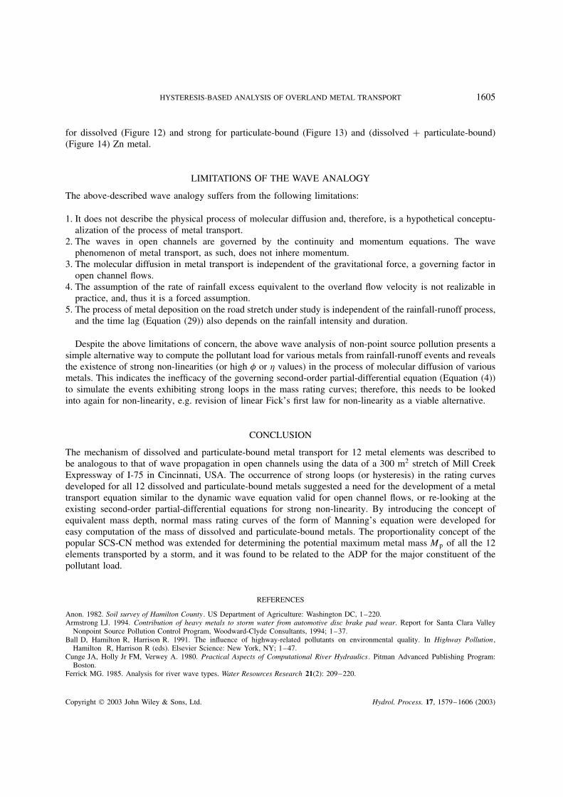
where Ma and Mp correspond to the total actual and potential mass of the metal element in an eventrespectively. Taking Ia D 0Ð0 in Equation (34), Mp can be computed for a known Q (direct surface runoff),P (rainfall), and actual mass Ma of the metal under study. The variables in Equations (33) and (34) aredistinguished from the above in the sense that these represent the total mass, the rainfall, or the runoff ofthe complete storm event, rather than their temporal distributions during a storm. The values of Mp werecomputed for all events utilizing the data reported by Sansalone and Buchberger (1997), Sansalone et al.(1998), and Li et al. (1999). Their variation with the antecedent dry period (ADP) is shown in Figures 12–14for dissolved, particulate-bound, and (dissolved C particulate-bound) metals respectively for the event of 8August 1996. Apparently, except for Zn, all other metals generally exhibit a similar trend of variation; Mp

first increases with ADP, reaches a peak, and then approaches zero with increasing dry period. On the otherhand, Zn metal, a major constituent, exhibits a distinguished and convincing (though apparently hysteretic)behaviour with ADP in all its three forms of dissolved, particulate-bound, and dissolved C particulate-bound.For this metal, Mp is generally found to increase with ADP. It is worth mentioning that Mp is analogousto the SCS-CN parameter S, and ADP to the antecedent moisture condition. The hysteretic relation is mild



0.E+001.E+032.E+033.E+034.E+03

0 100 200 300 400 500 600

Antecedent dry period (ADP) (hr)

Mp o

f Z

n (

µg)

0 100 200 300 400 500 600


Mp o

f C

r (µ

g)

0.E+002.E+014.E+016.E+018.E+01

0 100 200 300 400 500 600


Mp o

f C

d (

µg)

0.E+00

1.E+01

2.E+01

3.E+01

0 100 200 300 400 500 600

Antecedent dry period (ADP) (hr)M

p o

f M

g (

µg)

0.E+001.E+032.E+033.E+034.E+03

0 100 200 300 400 500 600


Mp o

f P

b (

µg)

0.E+005.E+011.E+022.E+022.E+02

0 100 200 300 400 500 600


Mp o

f A

l (µg

)

0.E+00

5.E+02

1.E+03

2.E+03

0 100 200 300 400 500 600


Mp o

f N

i (µg

)

0.E+001.E+012.E+013.E+014.E+01

0 100 200 300 400 500 600


Mp o

f C

a (µ

g)

0.E+00

2.E+04

4.E+04

6.E+04

0 100 200 300 400 500 600


Mp o

f M

n (

µg)

0.E+001.E+022.E+023.E+024.E+025.E+02

0 100 200 300 400 500 600


Mp o

f C

u

0.E+00

5.E+01

1.E+02

2.E+02

0 100 200 300 400 500 600


Mp o

f F

e (µ

g)

0.E+00

2.E+02

4.E+02

6.E+02

Figure 12. Behaviour of the potential maximum mass Mp of dissolved solids ��g� with the ADP



0.E+00

5.E+02

1.E+03

2.E+03

0 100 200 300 400 500 600


Mp o

f Z

n (

µg)

0.E+005.E+011.E+022.E+022.E+02

0 100 200 300 400 500 600


Mp o

f C

r (µ

g)

0 100 200 300 400 500 600


0.E+005.E+001.E+012.E+012.E+01

Mp o

f C

d (

µg)

0 100 200 300 400 500 600


p o

f M

g (

µg)

0.E+00

5.E+02

1.E+03

0 100 200 300 400 500 600


Mp o

f P

b (

µg)

0.E+001.E+022.E+023.E+024.E+02

0 100 200 300 400 500 600


Mp o

f A

I (µg

)

0.E+005.E+031.E+042.E+042.E+04

0 100 200 300 400 500 600


Mp o

f N

i (µg

)

0.E+001.E+012.E+013.E+014.E+015.E+01

0 100 200 300 400 500 600


Mp o

f C

a (µ

g)

0.E+001.E+032.E+033.E+034.E+03

0 100 200 300 400 500 600


Mp o

f M

n (

µg)

0.E+001.E+022.E+023.E+024.E+025.E+02

0 100 200 300 400 500 600


Mp o

f C

u

0.E+005.E+011.E+022.E+022.E+023.E+02

0 100 200 300 400 500 600


Mp o

f F

e (µ

g)

0.E+00

1.E+04

2.E+04

3.E+04

0 100 200 300 400 500 600


Mp o

f N

a (µ

g)

0.E+00

5.E+02

1.E+03

2.E+03

Figure 13. Behaviour of the potential maximum mass Mp of particulate-bound solids ��g� with the ADP



0.E+001.E+032.E+033.E+034.E+03

0 100 200 300 400 500 600


Mp o

f Z

n (

µg)

0.E+00

1.E+02

2.E+02

3.E+02

0 100 200 300 400 500 600


Mp o

f C

r (µ

g)

0 100 200 300 400 500 600


Mp o

f C

d (

µg)

0.E+00

2.E+01

4.E+01

6.E+01

0 100 200 300 400 500 600


p o

f M

g (

µg)

0.E+001.E+032.E+033.E+034.E+03

0 100 200 300 400 500 600


Mp o

f P

b (

µg)

0.E+00

2.E+02

4.E+02

6.E+02

0 100 200 300 400 500 600


Mp o

f A

l (µg

)

0.E+005.E+031.E+042.E+042.E+04

0 100 200 300 400 500 600


Mp o

f N

i (µg

)

0.E+00

5.E+01

1.E+02

0 100 200 300 400 500 600


Mp o

f C

a (µ

g)

0.E+00

2.E+04

4.E+04

6.E+04

0 100 200 300 400 500 600


Mp o

f M

n (

µg)

0.E+00

5.E+02

1.E+03

0 100 200 300 400 500 600


Mp o

f C

u

0.E+001.E+022.E+023.E+024.E+02

0 100 200 300 400 500 600


Mp o

f F

e (µ

g)

0.E+00

1.E+04

2.E+04

3.E+04

0 100 200 300 400 500 600


0.E+00

2.E+04

4.E+04

6.E+04

Har

dn

ess

Mp

Figure 14. Behaviour of the potential maximum mass Mp of total �dissolved C particulate-bound� solids with the ADP



for dissolved (Figure 12) and strong for particulate-bound (Figure 13) and (dissolved C particulate-bound)(Figure 14) Zn metal.

LIMITATIONS OF THE WAVE ANALOGY

The above-described wave analogy suffers from the following limitations:

1. It does not describe the physical process of molecular diffusion and, therefore, is a hypothetical conceptu-alization of the process of metal transport.

2. The waves in open channels are governed by the continuity and momentum equations. The wavephenomenon of metal transport, as such, does not inhere momentum.

3. The molecular diffusion in metal transport is independent of the gravitational force, a governing factor inopen channel flows.

4. The assumption of the rate of rainfall excess equivalent to the overland flow velocity is not realizable inpractice, and, thus it is a forced assumption.

5. The process of metal deposition on the road stretch under study is independent of the rainfall-runoff process,and the time lag (Equation (29)) also depends on the rainfall intensity and duration.

Despite the above limitations of concern, the above wave analysis of non-point source pollution presents asimple alternative way to compute the pollutant load for various metals from rainfall-runoff events and revealsthe existence of strong non-linearities (or high � or � values) in the process of molecular diffusion of variousmetals. This indicates the inefficacy of the governing second-order partial-differential equation (Equation (4))to simulate the events exhibiting strong loops in the mass rating curves; therefore, this needs to be lookedinto again for non-linearity, e.g. revision of linear Fick’s first law for non-linearity as a viable alternative.

CONCLUSION

The mechanism of dissolved and particulate-bound metal transport for 12 metal elements was described tobe analogous to that of wave propagation in open channels using the data of a 300 m2 stretch of Mill CreekExpressway of I-75 in Cincinnati, USA. The occurrence of strong loops (or hysteresis) in the rating curvesdeveloped for all 12 dissolved and particulate-bound metals suggested a need for the development of a metaltransport equation similar to the dynamic wave equation valid for open channel flows, or re-looking at theexisting second-order partial-differential equations for strong non-linearity. By introducing the concept ofequivalent mass depth, normal mass rating curves of the form of Manning’s equation were developed foreasy computation of the mass of dissolved and particulate-bound metals. The proportionality concept of thepopular SCS-CN method was extended for determining the potential maximum metal mass Mp of all the 12elements transported by a storm, and it was found to be related to the ADP for the major constituent of thepollutant load.

REFERENCES

Anon. 1982. Soil survey of Hamilton County . US Department of Agriculture: Washington DC, 1–220.Armstrong LJ. 1994. Contribution of heavy metals to storm water from automotive disc brake pad wear. Report for Santa Clara Valley

Nonpoint Source Pollution Control Program, Woodward-Clyde Consultants, 1994; 1–37.Ball D, Hamilton R, Harrison R. 1991. The influence of highway-related pollutants on environmental quality. In Highway Pollution ,

Hamilton R, Harrison R (eds). Elsevier Science: New York, NY; 1–47.Cunge JA, Holly Jr FM, Verwey A. 1980. Practical Aspects of Computational River Hydraulics . Pitman Advanced Publishing Program:

Boston.Ferrick MG. 1985. Analysis for river wave types. Water Resources Research 21(2): 209–220.



Fread DL. 1984, 1985. Dam break flood forecasting model (DAMBRK), User Manual. National Weather Service, Maryland, USA.French RH. 1985. Open Channel Hydraulics . McGraw-Hill: New York, NY; 551.Hayden HW, Moffatt WG, Wulff J. 1986. The Structure and Properties of Materials: Mechanical Behaviour, vol. III. Wiley Eastern Limited:

New Delhi, India.Henderson FM. 1966. Open Channel Flow . Macmillan: New York, USA.Jain MK, Mishra SK, Seth SM. 1996. Hysteresis criteria for the applicability of CPC and CPMC methods of flood routing. In Proceedings

of International Conference on Disasters and Mitigation, Anna University, Madras (India), 19–22 January.Kobriger NP, Geinopolos A. 1984. Sources and migration of highway runoff pollutants—research report, volume III. Report FHWA/RD-

84/059 (PB86-227915) FHWA, US Department of Transportation.Kundzewicz ZW, Dooge JCI. 1989. Attenuation and phase shift in linear flood routing. Hydrological Sciences Journal 34(1): 21–40.Li Y, Buchberger SG, Sansalone JJ. 1999. Variably saturated flow in storm-water partial exfiltration trench. Journal of Environmental

Engineering, ASCE 125(6): 556–565.Lygren E, Gjessing E, Berglind L. 1984. Pollution transport from a highway. The Science of the Total Environment 33: 147–159.Martin JL, McCutcheon SC. 1999. Hydrodynamics and Transport for Water Quality Modeling . Lewis Publishers: New York, NY.Menendez AN, Norscini R. 1982. Spectrum of shallow water waves: an analysis. Journal of the Hydraulics Division, ASCE 108(HY1):

75–94.Menendez AN, Norscini R. 1983. Discussion on ‘Nature of flood wave attenuation in open channel flow. Journal of the Hydraulics Division,

ASCE 109(5): 786–789.Mishra SK. 1998. Operation of a multipurpose reservoir. PhD thesis, University of Roorkee, UP, India.Mishra SK, Seth SM. 1994. Effect of downstream boundary conditions on dam break flood wave propagation characteristics. Technical

Report, National Institute of Hydrology, Roorkee (India).Mishra SK, Seth SM. 1996. Use of hysteresis for defining the nature of flood wave propagation in natural channels. Hydrological Sciences

Journal–Journal des Sciences Hydrologiques 41(2): 153–170.Mishra SK, Singh VP. 1999a. Hysteresis-based flood wave analysis. Journal of Hydrologic Engineering, ASCE 4(4): 358–365.Mishra SK, Singh VP. 1999b. Another look at the SCS-CN method. Journal of Hydrologic Engineering, ASCE 4(3): 257–264.Mishra SK, Singh VP. 2001. On Seddon speed formula. Journal of Hydrological Sciences 46(2): 333–347.Mishra SK, Sah S, Sharma N, Seth SM. 1996. Defining flood wave propagation characteristics using hysteresis of rating curves. In

HYDRO96, 11–13 December, IIT, Kanpur, India.Mishra SK, Jain MK, Seth SM. 1997. Characterization of flood waves by rating curves. Journal of Nordic Hydrology 28(1): 51–64.Muschack W. 1990. Pollution of street run-off by traffic and local conditions. The Science of the Total Environment 93: 419–431.Perumal M. 1994. Hydrodynamic derivation of a variable parameter Muskingum method: 2. Verification. Hydrological Sciences Journal

39(5): 443–458.Ponce VM. 1989. Engineering Hydrology: Principles and Practices . Prentice Hall: Englewood Cliffs, NJ.Ponce VM, Simons DB. 1977. Shallow wave propagation in open channel flow. Journal of the Hydraulics Division, ASCE 103(HY12):

1461–1476.Ponce VM, Lohani AK, Scheyhing C. 1996. Analytical verification of Muskingum–Cunge routing. Journal of Hydrology 174: 235–241.Price RK. 1973. Flood routing methods in British rivers. Proceedings of the Institution Civil Engineers (London), Part 2 57: 913–930.Price RK. 1985. Flood routing. In Developments in Hydraulic Engineering , Novak EJP (ed.). Elsevier Applied Science.Rutschmann P, Hager WH. 1996. Diffusion of flood waves. Journal of Hydrology 178: 19–32.SCS. 1956. Hydrology. In National Engineering Handbook, Supplement A. Soil Conservation Service, USDA: Washington, DC; Section 4,

Chapter 10.Sansalone JJ, Buchberger WH. 1997. Partitioning and first flush of metals in urban roadway storm water. Journal of Environmental

Engineering, ASCE 123(2): 134–143.Sansalone JJ, Tribouillard T. 1999. Variation in characteristics of abraded roadway particles as a function of particle size—implications for

water quality and drainage. In Transportation Research Record 1690 . TRB, National Research Council: Washington, DC; 153–163.Sansalone JJ, Koran JM, Smithson JA, Buchberger SG. 1998. Physical characteristics of urban roadway solids transported during rain events.

Journal of Environmental Engineering, ASCE 125(6): 556–565.Singh VP. 1996. Kinematic Wave Modelling in Water Resources: Surface Water Hydrology . John Wiley & Sons: New York.Singh VP. 1988. Hydrologic Systems: Vol. 1. Rainfall-Runoff Modelling . Prentice Hall: Englewood Cliffs, NJ.


Documents

Hysteresis-based analysis of overland metal transport